GROMACS Tutorial

GROMACS Introductory Tutorial

Adapted from:

Author: John E. Kerrigan, Ph.D.Associate Director, BioinformaticsThe Cancer Institute of NJ195 Little Albany StreetNew Brunswick, NJ 08903Phone: (732) 235-4473

GROMACS Tutorial for Solvation Study of Spider Toxin Peptide.

Yu, H., Rosen, M. K., Saccomano, N. A., Phillips, D., Volkmann, R. A., Schreiber, S. L.: Sequential assignment and structure determination of spider toxin omega-Aga-IVB. Biochemistry 32 pp. 13123 (1993)

GROMACS is a high-end, high performance research tool designed for the study of protein dynamics using classical molecular dynamics theory.[1, 2] This versatile software package is Gnu public license free software. You may download it from http://www.gromacs.org. GROMACS runs on linux, unix, and on Windows (a recent development).

Synopsis

In this tutorial, you will study a toxin isolated from the venom of the funnel web spider. Venom toxins have been used in the past to identify cation channels. Calcium ion channels regulate the entry of this ion into cells. Nerve signals are highly governed by the balance of ions in neuronal cells. It is hypothesized that exposed positively charged residues in venoms like the spider toxin here bind favorably to the negatively charged entrance of the cell's ion channel. The spider toxin in this tutorial has its positively charged residues pointing predominantly to one side of the peptide. The ion channel is blocked, resulting in blocked nerve signal leading to paralysis and ultimately to death (presumably via respiratory failure).

We will study this peptide toxin using explicit solvation dynamics. We will solvate the peptide in a water box followed by equilibration using Newton's laws of motion. We will neutralize the system by adding counterions. We will evaluate the contributions of potential and kinetic energies to the total energy. We will analyze the stability of the tertiary and secondary structure of the protein during simulation.

Note: You will generate structure files in this tutorial. To view these files, you must use VMD

PDB file

Download 1OMB.PDB from the Protein Data Bank ( http://www.rcsb.org/pdb/ ).

Create a subdirectory in your unix account called "fwspider". Download the 1OMB.pdb from the PDB Databank using the following command...

wget http://www.rcsb.org/pdb/files/1OMB.pdb

Gromacs input preparation

1. Process the pdb file with pdb2gmx

The pdb2gmx command converts your pdb file to a gromacs file and writes the topology for you. This file is derived from an NMR structure which contains hydrogen atoms. Therefore, we use the -ignh flag to ignore hydrogen atoms in the pdb file. The -ff flag is used to select the forcefield (G43a1 is the Gromos 96 FF, a united atom FF). The -f flag reads the pdb file. The -o flag outputs a new pdb file (various file formats supported) with the name you have given it in the command line. The -p flag is used for output and naming of the topology file. The topology file is very important as it contains all of the forcefield parameters (based upon the forcefield that you select in the initial prompt) for your model. Studies have revealed that the SPC/E water model [3] performs best in water box simulations. [4] Use the spce water model as it is better for use with the long-range electrostatics methods. So, we use the -water flag to specify this model.

pdb2gmx -ignh -ff gromos43a1 -f 1OMB.pdb -o fws.pdb -p fws.top -water spce

2. Setup the Box for your simulations

editconf -bt octahedron -f fws.pdb -o fws-b4sol.pdb -d 1.0

What you have done in this command is specify that you want to use a truncated octahedron box. The -d 1.0 flag sets the dimensions of the box based upon setting the box edge approx 1.0 nm (i.e. 10.0 angstroms) from the molecule(s) periphery. Ideally you should set -d at no less than 0.9 nm for most systems. [5]

[Special Note: editconf may also be used to convert gromacs files (*.gro) to pdb files (*.pdb) and vice versa. For example: editconf -f file.gro -o file.pdb converts file.gro to the pdb file file.pdb]

3. Solvate the box

genbox -cp fws-b4sol.pdb -cs spc216.gro -o fws-b4ion.pdb -p fws.top

The genbox command generates the water box based upon the dimensions/box type that you had specified using editconf. In the command above, we specify the spc water box. The genbox program will add the correct number of water molecules needed to solvate your box of given dimensions.

Preparation for running calculations

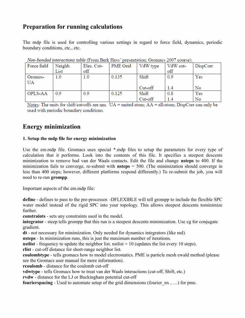
The mdp file is used for controlling various settings in regard to force field, dynamics, periodic boundary conditions, etc., etc.

Energy minimization

1. Setup the mdp file for energy minimization

Use the em.mdp file. Gromacs uses special *.mdp files to setup the parameters for every type of calculation that it performs. Look into the contents of this file. It specifies a steepest descents minimization to remove bad van der Waals contacts. Edit the file and change nsteps to 400. If the minimization fails to converge, re-submit with nsteps = 500. (The minimization should converge in less than 400 steps; however, different platforms respond differently.) To re-submit the job, you will need to re-run grompp.

Important aspects of the em.mdp file:

define - defines to pass to the pre-processor. -DFLEXIBLE will tell grompp to include the flexible SPC water model instead of the rigid SPC into your topology. This allows steepest descents tominimize further.constraints - sets any constraints used in the model.integrator - steep tells grompp that this run is a steepest descents minimization. Use cg for conjugate gradient. dt - not necessary for minimization. Only needed for dynamics integrators (like md).nsteps - In minimization runs, this is just the maximum number of iterations.nstlist - frequency to update the neighbor list. nstlist = 10 (updates the list every 10 steps).rlist - cut-off distance for short-range neighbor list.coulombtype - tells gromacs how to model electrostatics. PME is particle mesh ewald method (please see the Gromacs user manual for more information).rcoulomb - distance for the coulomb cut-offvdwtype - tells Gromacs how to treat van der Waals interactions (cut-off, Shift, etc.)rvdw - distance for the LJ or Buckingham potential cut-offfourierspacing - Used to automate setup of the grid dimensions (fourier_nx , …) for pme.

EM Stuffemtol - the minimization converges when the max force is smaller than this value (in units of kJmol-1 nm-1)emstep - initial step size (in nm).

2. Create the tpr file

Now process the files with grompp. grompp is the pre-processor program (the gromacs preprocessor “grompp” Get it! Sigh!). grompp will setup your run for input into mdrun.

grompp -f em.mdp -c fws-b4ion.pdb -p fws.top -o ion.tpr -maxwarn 5

The -f flag in grompp is used to input the parameter file (*.mdp). The -c flag is used to input the coordinate file (the pdb file, *.pdb); -p inputs the topology and -o outputs the input file (*.tpr) needed for mdrun.

3. Add ions to neutralize the system

You may use the tpr file generated here to add counterions to your model to neutralize any net charge. In order for the Ewald equation we are using to describe long range electrostatics in our model to be valid, the net system charge must be neutral. Our model has a net charge of +2.00. Therefore, we want to add two chloride ions. Use the genion command to add the chloride ions.

genion -s ion.tpr -o fws-b4em.pdb -nname CL -nn 2 -p fws.top -g ion.log

Where -nname is the negative ion name (CL for the Gromos G43a1 force field; see the ions.itp file for specifics wrt force field), -nn is the number of negative ions to add. Use -pname to add positively charged ions and -np to specify the number of positively charged ions to add. The -g flag gives a name to the output log for genion.

An even easier method which creates a neutral system using a specified concentration of NaCl uses the -neutral and -conc flags as in the following …

genion -s ion.tpr -o fws-b4em.pdb -neutral -conc 0.15 -p fws.top -g ion.log

We will use the 0.15 M NaCl model via the command above. The -norandom flag places ions based on electrostatic potential as opposed to random placement (default). However, we will use the default (random placement). When you process this command, you will be prompted to provide a continuous group of solvent molecules, which should be Group 13 (SOL). Type 13 then <enter>. You will notice that a number of solvent molecules have been replaced by Na and Cl ions. You should also notice that the fws.top file has been updated to include the NA and CL ions in your topology accounting for the replaced water molecules.

Caution: The molecules listed here must appear in the exact same order as in your coordinate file!

4. Regenerate the tpr file with ions included

If you added the chloride ions, you will need to run the grompp step again. First remove the old fws_em.tpr file, then run the next grompp command below. We added chloride ions in our model to

neutralize the overall net charge of the model.

grompp -f em.mdp -c fws-b4em.pdb -p fws.top -o em.tpr -maxwarn 5

5. Run the energy minimization

mdrun -v -deffnm em

Use the tail command to check on the progress of the minimization.

tail -15 em.log

When the minimization is complete, you should see the following summary in your log file indicating that steepest descents converged. Use tail -100 em.log

Steepest Descents converged to Fmax < 1000 in 240 stepsPotential Energy = -1.9688684e+05Maximum force = 9.9480914e+02 on atom 106Norm of force = 5.4587994e+01

Position-restrained simulation

1. Setup the mdp file for energy minimization

Setup the position-restrained molecular dynamics. What is position-restrained MD? You are restraining (or partially freezing, if you will) the atom positions of the macromolecule while letting the solvent move in the simulation. This is done to “soak” the water molecules into the macromolecule. The relaxation time of water is ~ 10 ps. Therefore, we need to do dynamics in excess of 10 ps for position-restrained work. This example uses a 50.0 ps time scale (at least an order of magnitude greater. Larger models (large proteins/lipids) may require longer preequilibration periods of 50 or 100 ps or more. The settings below are recommended for the Gromacs/Gromos forcefields. Under coulombtype, PME stands for “Particle Mesh Ewald” electrostatics. [6, 7] PME is the best method for computing long-range electrostatics (gives more reliable energy estimates especially for systems where counterions like Na+, Cl-, Ca 2+ , etc. are used). Due to the nature of this particular protein having exposed charged residues with a net +2 charge to the system, it is beneficial for us to use PME. It is even more beneficial for us to use counterions to balance the charge and set the system to net neutral; otherwise, PME will not give reliable results. The all-bonds option under constraints applies the Linear Constraint algorithm for fixing all bond lengths in the system (important to use this option when dt > 0.001 ps). [8] Study the mdp file below.

Important things to know about the mdp file:

– The -DPOSRES in the define statement tells Gromacs to perform position restrained dynamics.– The constraints statement is as previously discussed. all-bonds sets the LINCS constraint for

all bonds. [8]– - The integrator tells gromacs what type of dynamics algorithm to use (another option is “sd”

for stochastic dynamics).– dt is the time step (we have selected 2 fs; however, this must be entered in units of ps!). nsteps

is the number of steps to run (just multiply nsteps X dt to compute the length of the simulation).– nstxout tells gromacs how often to collect a “snapshot” for the trajectory. (e.g. nstxout = 250

with dt = 0.002 would collect a snapshot every 0.5 ps)– coulombtype selects the manner in which Gromacs computes electrostatic interactions between

atoms. (PME is particle mesh ewald; there are other options like cut-off).– rcoulomb and rvdw are the cutoffs (in nm; 1.0 nm = 10.0 angstroms) for the electrostatic and

van der Waals terms.

The temperature coupling section is very important and must be filled out correctly.

– Tcoupl = v-rescale [9, 10] (type of temperature coupling where velocity is rescaled using a stochastic term.)

– tau_t = Time constant for temperature coupling (units = ps). You must list one per tc_grp in the order in which tc_grps appear.

– tc_grps = groups to couple to the thermostat (every atom or residue in your model must be represented here by appropriate index groups).

– ref_t = reference temperature for coupling (i.e. the temperature of your MD simulation in degrees K). You must list one per tc_grp in the order in which tc_grps appear.

– When you alter the temperature, don’t forget to change the gen_temp variable for velocity generation.

– pcoupltype - isotropic means that the “box” will expand or contract evenly in all directions (x, y,and z) in order to maintain the proper pressure. Note: Use semiisotropic for membrane simulations.

– tau_p - time constant for coupling (in ps).– compressibility - this is the compressibility of the solvent used in the simulation in bar-1 (the

setting above is for water at 300 K and 1 atm).– ref_p - the reference pressure for the coupling (in bar) (1 atm ~ 0.983 bar).– gen_seed = -1 Use random number seed based on process ID #. More important for Langevin

dynamics.[11]

2. Create the tpr file and start the simulation

grompp -f pr.mdp -c em.gro -p fws.top -o pr.tpr -maxwarn 5

nohup mdrun -deffnm pr &

Use the tail command to check the pr.log file.

Production run simulation

The md.mdp parameter file looks very similar to the pr.mdp file. There are several differences. The define statement is not necessary as we are not running as position restrained dynamics.

1. Check parameters in the mdp file, create the tpr file and start the simulation

grompp -f md.mdp -c pr.gro -p fws.top -o md.tpr -maxwarn 3

nohup mdrun -deffnm md &

Use the tail command to check the md.log file.

You may compress the trajectory using trjconv to save on disk space. Note - we set nstxtcout = 500; therefore, you should already have a compressed copy of your trajectory. However, for display purposes, you might need to use “ -pbc nojump” to keep everything in the box.

trjconv -f md.trr -s md.tpr -o md.xtc -pbc nojump -ur compact -center

Once you have made the *.xtc file, you may delete the *.trr file.

Use VMD to view the trajectory

vmd em.gro md.xtc &

Create different representations for protein, water and ions. To view the animation of the MD trajectory click on the “play forward” button in the lower right corner.

Exercise 1: Using VMD generate a movie with the trajectory animation. For this, use the Movie Generator tool from Extensions/Visualization menu. Change the Movie Settings to trajectory and use Snapshot for rendering. (Tip: for smooth protein motion go to Graphical Representations and increase the smoothing window from the Trajectory section to 5 for the protein.)

Analysis

One of the major advantages of Gromacs (other than the fact that it is GNU public domain and free!) is the robust set of programs available for analyzing the trajectories. We will discuss a few of the more important analytic tools in the Gromacs arsenal here.

1. Extract energy components

g_energy

Use this program to plot energy data, pressure, volume, density, etc.

g_energy -f md.edr -s md.tpr -o fws_pe.xvg

You will be prompted for the specific data that you want to include in the output file (*.xvg). For Potential energy, type 10 <enter>Hit the <enter> key again

The output file is a type of spreadsheet file that can be read using Xmgrace. This file is a text file and can be read into Microsoft Excel; however, you will need to do some light editing of the file.

To read *.xvg files into Grace use the following command:

xmgrace -nxy fws_pe.xvg

Potential energy plot of whole system.

Exercise 2: What is the average potential energy for the entire simulation?Exercise 3: Extract and plot the total and kinetic energies. How do they compare to the potential energy?

2. Calculate the root mean square deviation (rmsd)

RMSD can give information about the convergence of the simulation and protein stability. Use g_rms to evaluate the deviation of the structure from the original starting structure over the course of the simulation. To compare rmsd to the NMR structure use the following command …

g_rms -s em.tpr -f md.trr -o fws_rmsd.xvg

Select group 4 (Backbone) for the least squares fit and output. The program will generate a plot of rmsd over time (rmsd.xvg) which you may be plotted with Xmgrace.

xmgrace -nxy fws_pe.xvg

The example above is the result of our 500 ps simulation.

An Aside: Has my Protein Equilibrated after my Production Run?

This is an often-asked question on discussion lists. The answer really depends upon the property(ies) you are studying. Overall potential energy tends to be noisy and is a deceptive measure of system equilibration. Protein backbone RMSD will give an indication of stability in the overall backbone, but what about a loop region? You might need to zero-in on the region of interest in your analysis to be sure. You will also need to know the approximate time scale of the property you are studying to really know whether or not you have run your production dynamics for a long enough period of time (for example, protein folding events can run the gamut of a few microseconds to minutes and even as long as hours in terms of timescales!).

Exercise 4: Calculate the RMSD using all the atoms of the protein. How does it compare to the RMSD of the backbone?

3. Identify the secondary structure of the protein

Use the do_dssp command to analyze the secondary structure of your model.[12]

do_dssp -s md.tpr -f md.trr -b 400 -e 500 -o fws_ss.xpm

Select Group 1 (Protein) for the calculation. Use the xpm2ps program to convert the xpm file to eps format. Then use the Gimp to view the eps file and convert it to jpg or whatever desired image format.

xpm2ps -f fws_ss.xpm -o fws_ss.epsgimp fws_ss.eps

Exercise 4: Which residues have β-sheet conformation? Using VMD generate an image with the protein in the “new cartoon” representation and coloring based on “structure”. Do the β-sheet residues match the ones from the dssp plot?

References