Embed Size (px)
Citation preview
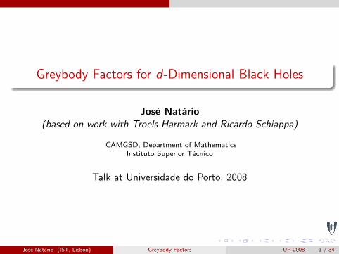
Greybody Factors for d-Dimensional Black Holes
Jose Natario(based on work with Troels Harmark and Ricardo Schiappa)
CAMGSD, Department of MathematicsInstituto Superior Tecnico
Talk at Universidade do Porto, 2008
Jose Natario (IST, Lisbon) Greybody Factors UP 2008 1 / 34

Outline
1 IntroductionWhat are Greybody Factors?How to compute them?Why do we care?
2 Low FrequencyMethodResults
Asymptotically Flat SolutionsAsymptotically de Sitter SolutionsAsymptotically Anti de Sitter Solutions
3 High Imaginary FrequencyMethodResults
Asymptotically Flat SolutionsAsymptotically Flat SolutionsAsymptotically de Sitter SolutionsAsymptotically Anti de Sitter Solutions
Jose Natario (IST, Lisbon) Greybody Factors UP 2008 2 / 34
Introduction What are Greybody Factors?
Outline
1 IntroductionWhat are Greybody Factors?How to compute them?Why do we care?
2 Low FrequencyMethodResults
Asymptotically Flat SolutionsAsymptotically de Sitter SolutionsAsymptotically Anti de Sitter Solutions
3 High Imaginary FrequencyMethodResults
Asymptotically Flat SolutionsAsymptotically Flat SolutionsAsymptotically de Sitter SolutionsAsymptotically Anti de Sitter Solutions
Jose Natario (IST, Lisbon) Greybody Factors UP 2008 3 / 34

Introduction What are Greybody Factors?
What are Greybody Factors?
Consider the massless wave equation
Φ = 0
on a d-dimensional spherically symmetric black hole background:
ds2 = −f (r)dt2 + f (r)−1dr2 + r2dΩd−22.
Here
f (r) = 1−2µ
rd−3+
θ2
r2d−6− λr2
and
M =(d − 2) Ωd−2
8πGd
µ, Ωn =2π
n+12
Γ“
n+12
” ,Q2 =
(d − 2) (d − 3)
8πGd
θ2,
Λ =1
2(d − 1) (d − 2) Λ.
Jose Natario (IST, Lisbon) Greybody Factors UP 2008 4 / 34

Introduction What are Greybody Factors?
What are Greybody Factors?
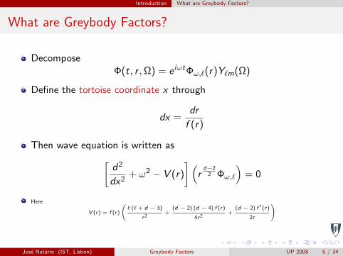
DecomposeΦ(t, r ,Ω) = e iωtΦω,`(r)Y`m(Ω)
Define the tortoise coordinate x through
dx =dr
f (r)
Then wave equation is written as[d2
dx2+ ω2 − V (r)
](r
d−22 Φω,`
)= 0
Here
V (r) = f (r)
` (` + d − 3)
r2+
(d − 2) (d − 4) f (r)
4r2+
(d − 2) f ′(r)
2r
!
Jose Natario (IST, Lisbon) Greybody Factors UP 2008 5 / 34

Introduction What are Greybody Factors?
What are Greybody Factors?
DecomposeΦ(t, r ,Ω) = e iωtΦω,`(r)Y`m(Ω)
Define the tortoise coordinate x through
dx =dr
f (r)
Then wave equation is written as[d2
dx2+ ω2 − V (r)
](r
d−22 Φω,`
)= 0
Here
V (r) = f (r)
` (` + d − 3)
r2+
(d − 2) (d − 4) f (r)
4r2+
(d − 2) f ′(r)
2r
!
Jose Natario (IST, Lisbon) Greybody Factors UP 2008 5 / 34

Introduction What are Greybody Factors?
What are Greybody Factors?
Potentials for d = 6 and ` = 0 in Schwarzschild, Schwarzschild-deSitter and Schwarzschild-Anti de Sitter:
Jose Natario (IST, Lisbon) Greybody Factors UP 2008 6 / 34

Introduction What are Greybody Factors?
What are Greybody Factors?
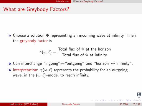
Choose a solution Φ representing an incoming wave at infinity. Thenthe greybody factor is
γ(ω, `) =Total flux of Φ at the horizon
Total flux of Φ at infinity
Can interchange “ingoing”↔“outgoing” and “horizon”↔“infinity”.
Interpretation: γ(ω, `) represents the probability for an outgoingwave, in the (ω, `)–mode, to reach infinity.
Jose Natario (IST, Lisbon) Greybody Factors UP 2008 7 / 34

Introduction What are Greybody Factors?
What are Greybody Factors?
Choose a solution Φ representing an incoming wave at infinity. Thenthe greybody factor is
γ(ω, `) =Total flux of Φ at the horizon
Total flux of Φ at infinity
Can interchange “ingoing”↔“outgoing” and “horizon”↔“infinity”.
Interpretation: γ(ω, `) represents the probability for an outgoingwave, in the (ω, `)–mode, to reach infinity.
Jose Natario (IST, Lisbon) Greybody Factors UP 2008 7 / 34

Introduction What are Greybody Factors?
What are Greybody Factors?
Jose Natario (IST, Lisbon) Greybody Factors UP 2008 8 / 34

Introduction What are Greybody Factors?
What are Greybody Factors?
Jose Natario (IST, Lisbon) Greybody Factors UP 2008 9 / 34
Introduction What are Greybody Factors?
What are Greybody Factors?
Jose Natario (IST, Lisbon) Greybody Factors UP 2008 10 / 34
Introduction How to compute them?
Outline
1 IntroductionWhat are Greybody Factors?How to compute them?Why do we care?
2 Low FrequencyMethodResults
Asymptotically Flat SolutionsAsymptotically de Sitter SolutionsAsymptotically Anti de Sitter Solutions
3 High Imaginary FrequencyMethodResults
Asymptotically Flat SolutionsAsymptotically Flat SolutionsAsymptotically de Sitter SolutionsAsymptotically Anti de Sitter Solutions
Jose Natario (IST, Lisbon) Greybody Factors UP 2008 11 / 34
Introduction How to compute them?
How to compute them?
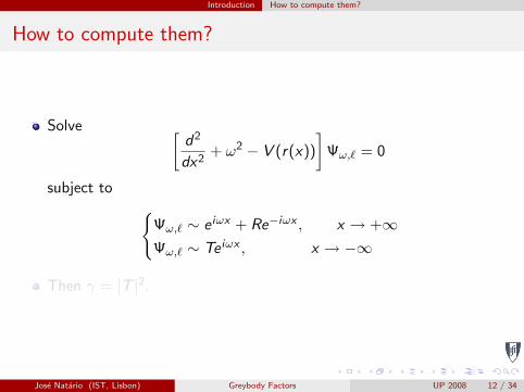
Solve [d2
dx2+ ω2 − V (r(x))
]Ψω,` = 0
subject to Ψω,` ∼ e iωx + Re−iωx , x → +∞Ψω,` ∼ Te iωx , x → −∞
Then γ = |T |2.
Jose Natario (IST, Lisbon) Greybody Factors UP 2008 12 / 34
Introduction How to compute them?
How to compute them?
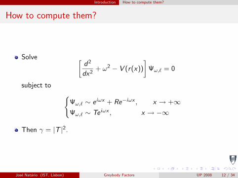
Solve [d2
dx2+ ω2 − V (r(x))
]Ψω,` = 0
subject to Ψω,` ∼ e iωx + Re−iωx , x → +∞Ψω,` ∼ Te iωx , x → −∞
Then γ = |T |2.
Jose Natario (IST, Lisbon) Greybody Factors UP 2008 12 / 34
Introduction Why do we care?
Outline
1 IntroductionWhat are Greybody Factors?How to compute them?Why do we care?
2 Low FrequencyMethodResults
Asymptotically Flat SolutionsAsymptotically de Sitter SolutionsAsymptotically Anti de Sitter Solutions
3 High Imaginary FrequencyMethodResults
Asymptotically Flat SolutionsAsymptotically Flat SolutionsAsymptotically de Sitter SolutionsAsymptotically Anti de Sitter Solutions
Jose Natario (IST, Lisbon) Greybody Factors UP 2008 13 / 34
Introduction Why do we care?
Why do we care?
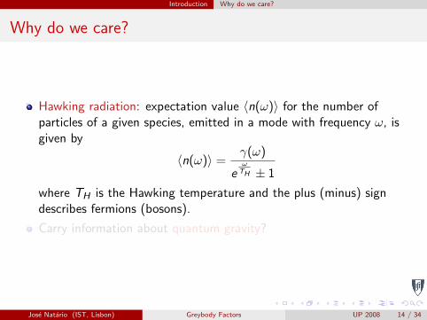
Hawking radiation: expectation value 〈n(ω)〉 for the number ofparticles of a given species, emitted in a mode with frequency ω, isgiven by
〈n(ω)〉 =γ(ω)
eω
TH ± 1
where TH is the Hawking temperature and the plus (minus) signdescribes fermions (bosons).
Carry information about quantum gravity?
Jose Natario (IST, Lisbon) Greybody Factors UP 2008 14 / 34

Introduction Why do we care?
Why do we care?
Hawking radiation: expectation value 〈n(ω)〉 for the number ofparticles of a given species, emitted in a mode with frequency ω, isgiven by
〈n(ω)〉 =γ(ω)
eω
TH ± 1
where TH is the Hawking temperature and the plus (minus) signdescribes fermions (bosons).
Carry information about quantum gravity?
Jose Natario (IST, Lisbon) Greybody Factors UP 2008 14 / 34
Low Frequency Method
Outline
1 IntroductionWhat are Greybody Factors?How to compute them?Why do we care?
2 Low FrequencyMethodResults
Asymptotically Flat SolutionsAsymptotically de Sitter SolutionsAsymptotically Anti de Sitter Solutions
3 High Imaginary FrequencyMethodResults
Asymptotically Flat SolutionsAsymptotically Flat SolutionsAsymptotically de Sitter SolutionsAsymptotically Anti de Sitter Solutions
Jose Natario (IST, Lisbon) Greybody Factors UP 2008 15 / 34
Low Frequency Method
Method
Split up spacetime into 3 regions:
Region I: The region near the (outer) event horizon, defined by r ' RH
and V (r) ω2.Region II: The intermediate region, defined by V (r) ω2.Region III: The asymptotic region, defined by r RH .
Solve wave equation for each region separately and match.
Assumed ` = 0.
Jose Natario (IST, Lisbon) Greybody Factors UP 2008 16 / 34
Low Frequency Results
Outline
1 IntroductionWhat are Greybody Factors?How to compute them?Why do we care?
2 Low FrequencyMethodResults
Asymptotically Flat SolutionsAsymptotically de Sitter SolutionsAsymptotically Anti de Sitter Solutions
3 High Imaginary FrequencyMethodResults
Asymptotically Flat SolutionsAsymptotically Flat SolutionsAsymptotically de Sitter SolutionsAsymptotically Anti de Sitter Solutions
Jose Natario (IST, Lisbon) Greybody Factors UP 2008 17 / 34
Low Frequency Results
ResultsAsymptotically Flat Solutions
γ(ω) =4πωd−2Rd−2
H
2d−2[Γ( d−12
)]2(RH = radius of the (outer) horizon).
Results best described in terms of the absorption cross section:
σ(ω) = γ(ω)|α|2
where α is the coefficient of the ` = 0 term in the decomposition of aplane wave into ingoing spherical harmonic waves.
We have the universal result
σ(ω) = AH
where AH is the area of the (outer) horizon.
First done in [Das, Gibbons and Mathur].
Jose Natario (IST, Lisbon) Greybody Factors UP 2008 18 / 34
Low Frequency Results
ResultsAsymptotically Flat Solutions
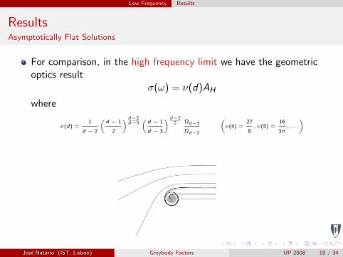
For comparison, in the high frequency limit we have the geometricoptics result
σ(ω) = ν(d)AH
where
ν(d) =1
d − 2
„d − 1
2
« d−2d−3
„d − 1
d − 3
« d−22 Ωd−3
Ωd−2
„ν(4) =
27
8, ν(5) =
16
3π, . . .
«
Jose Natario (IST, Lisbon) Greybody Factors UP 2008 19 / 34

Low Frequency Results
ResultsAsymptotically de Sitter Solutions
γ(ω) = 4h(ω)AHAC.
AH = area of the black hole horizonAC = area of the cosmological horizonω = frequency normalized by the cosmological radiush(ω) given by
h(ω) =
d−22Y
n=1
1 +
ω2
(2n − 1)2
!
for even d ≥ 4 and
h(ω) =πω
2coth
`πω2
´ d−32Y
n=1
1 +
ω2
(2n)2
!
for odd d ≥ 5.
Jose Natario (IST, Lisbon) Greybody Factors UP 2008 20 / 34
Low Frequency Results
ResultsAsymptotically de Sitter Solutions
Again universal result.
h(ω) = 1 as ω → 0, implying a nonzero greybody factor in this limit(cosmological horizon at a finite distance).
Jose Natario (IST, Lisbon) Greybody Factors UP 2008 21 / 34

Low Frequency Results
ResultsAsymptotically de Sitter Solutions
Again universal result.
h(ω) = 1 as ω → 0, implying a nonzero greybody factor in this limit(cosmological horizon at a finite distance).
Jose Natario (IST, Lisbon) Greybody Factors UP 2008 21 / 34
Low Frequency Results
ResultsAsymptotically de Sitter Solutions
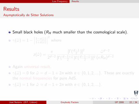
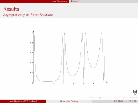
Small black holes (RH much smaller than the cosmological scale).
γ(ω) = 1−∣∣∣1−z(ω)
1+z(ω)
∣∣∣2 where
z(ω) =π
2d−2
[Γ(d−12 )]2
[Γ(d−1+ω2 )Γ(d−1−ω
2 )]2ωd−2
(κRH)d−2
Again universal result.
γ(ω) = 0 for ω = d − 1 + 2n with n ∈ 0, 1, 2, .... These are exactlythe normal frequencies for pure AdS.
γ(ω) = 1 for ω ' d − 1 + 2n with n ∈ 0, 1, 2, ....
Jose Natario (IST, Lisbon) Greybody Factors UP 2008 22 / 34
Low Frequency Results
ResultsAsymptotically de Sitter Solutions
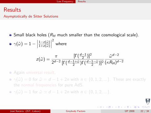
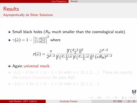
Small black holes (RH much smaller than the cosmological scale).
γ(ω) = 1−∣∣∣1−z(ω)
1+z(ω)
∣∣∣2 where
z(ω) =π
2d−2
[Γ(d−12 )]2
[Γ(d−1+ω2 )Γ(d−1−ω
2 )]2ωd−2
(κRH)d−2
Again universal result.
γ(ω) = 0 for ω = d − 1 + 2n with n ∈ 0, 1, 2, .... These are exactlythe normal frequencies for pure AdS.
γ(ω) = 1 for ω ' d − 1 + 2n with n ∈ 0, 1, 2, ....
Jose Natario (IST, Lisbon) Greybody Factors UP 2008 22 / 34

Low Frequency Results
ResultsAsymptotically de Sitter Solutions
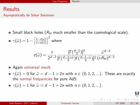
Small black holes (RH much smaller than the cosmological scale).
γ(ω) = 1−∣∣∣1−z(ω)
1+z(ω)
∣∣∣2 where
z(ω) =π
2d−2
[Γ(d−12 )]2
[Γ(d−1+ω2 )Γ(d−1−ω
2 )]2ωd−2
(κRH)d−2
Again universal result.
γ(ω) = 0 for ω = d − 1 + 2n with n ∈ 0, 1, 2, .... These are exactlythe normal frequencies for pure AdS.
γ(ω) = 1 for ω ' d − 1 + 2n with n ∈ 0, 1, 2, ....
Jose Natario (IST, Lisbon) Greybody Factors UP 2008 22 / 34
Low Frequency Results
ResultsAsymptotically de Sitter Solutions
0
0.2
0.4
0.6
0.8
1
1 2 3 4 5 6 7
Jose Natario (IST, Lisbon) Greybody Factors UP 2008 23 / 34
High Imaginary Frequency Method
Outline
1 IntroductionWhat are Greybody Factors?How to compute them?Why do we care?
2 Low FrequencyMethodResults
Asymptotically Flat SolutionsAsymptotically de Sitter SolutionsAsymptotically Anti de Sitter Solutions
3 High Imaginary FrequencyMethodResults
Asymptotically Flat SolutionsAsymptotically Flat SolutionsAsymptotically de Sitter SolutionsAsymptotically Anti de Sitter Solutions
Jose Natario (IST, Lisbon) Greybody Factors UP 2008 24 / 34

High Imaginary Frequency Method
Method
Complex ω:
Φ∗ω is replaced by Φ−ω.
R∗,T ∗ are replaced by R, T .RR + TT = 1.
ω → i∞: solve equation in the complex plane at origin, horizons,infinity; match solutions along (anti-)Stokes lines Re x = 0 and usemonodromies of Φω,Φ−ω at horizons to implement boundaryconditions.
Jose Natario (IST, Lisbon) Greybody Factors UP 2008 25 / 34
High Imaginary Frequency Method
Method
Jose Natario (IST, Lisbon) Greybody Factors UP 2008 26 / 34

High Imaginary Frequency Method
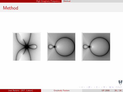
Method
Considered gravitational perturbations (tensor, vector, scalar) and any` (includes massless scalar field).Potentials are slightly more complicated: for example
VS(r) =f (r)U(r)
16r2H2(r),
where
H(r) = ` (` + d − 3)− (d − 2) +(d − 1) (d − 2) µ
rd−3,
and
U(r) = −"
4d (d − 1)2 (d − 2)3 µ2
r2d−6− 24 (d − 1) (d − 2)2 (d − 4)
n` (` + d − 3)− (d − 2)
o µ
rd−3+
+4 (d − 4) (d − 6)n` (` + d − 3)− (d − 2)
o2#λr2 + 8 (d − 1)2 (d − 2)4 µ3
r3d−9+ 4 (d − 1) (d − 2) ·
·"
4“
2d2 − 11d + 18”n
` (` + d − 3)− (d − 2)o
+ (d − 1) (d − 2) (d − 4) (d − 6)
#µ2
r2d−6− 24 (d − 2) ·
·"
(d − 6)n` (` + d − 3)− (d − 2)
o+ (d − 1) (d − 2) (d − 4)
#n` (` + d − 3)− (d − 2)
o µ
rd−3+
+16n` (` + d − 3)− (d − 2)
o3+ 4d (d − 2)
n` (` + d − 3)− (d − 2)
o2.
Jose Natario (IST, Lisbon) Greybody Factors UP 2008 27 / 34

High Imaginary Frequency Method
Method
Considered gravitational perturbations (tensor, vector, scalar) and any` (includes massless scalar field).Potentials are slightly more complicated: for example
VS(r) =f (r)U(r)
16r2H2(r),
where
H(r) = ` (` + d − 3)− (d − 2) +(d − 1) (d − 2) µ
rd−3,
and
U(r) = −"
4d (d − 1)2 (d − 2)3 µ2
r2d−6− 24 (d − 1) (d − 2)2 (d − 4)
n` (` + d − 3)− (d − 2)
o µ
rd−3+
+4 (d − 4) (d − 6)n` (` + d − 3)− (d − 2)
o2#λr2 + 8 (d − 1)2 (d − 2)4 µ3
r3d−9+ 4 (d − 1) (d − 2) ·
·"
4“
2d2 − 11d + 18”n
` (` + d − 3)− (d − 2)o
+ (d − 1) (d − 2) (d − 4) (d − 6)
#µ2
r2d−6− 24 (d − 2) ·
·"
(d − 6)n` (` + d − 3)− (d − 2)
o+ (d − 1) (d − 2) (d − 4)
#n` (` + d − 3)− (d − 2)
o µ
rd−3+
+16n` (` + d − 3)− (d − 2)
o3+ 4d (d − 2)
n` (` + d − 3)− (d − 2)
o2.
Jose Natario (IST, Lisbon) Greybody Factors UP 2008 27 / 34
High Imaginary Frequency Results
Outline
1 IntroductionWhat are Greybody Factors?How to compute them?Why do we care?
2 Low FrequencyMethodResults
Asymptotically Flat SolutionsAsymptotically de Sitter SolutionsAsymptotically Anti de Sitter Solutions
3 High Imaginary FrequencyMethodResults
Asymptotically Flat SolutionsAsymptotically Flat SolutionsAsymptotically de Sitter SolutionsAsymptotically Anti de Sitter Solutions
Jose Natario (IST, Lisbon) Greybody Factors UP 2008 28 / 34
High Imaginary Frequency Results
ResultsAsymptotically Flat Solutions
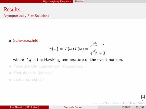
Schwarzschild:
γ(ω) = T (ω)T (ω) =eω
TH − 1
eω
TH + 3
where TH is the Hawking temperature of the event horizon.
Poles are the quasinormal frequencies.
First done in [Neitzke].
Exotic statistics?
Jose Natario (IST, Lisbon) Greybody Factors UP 2008 29 / 34

High Imaginary Frequency Results
ResultsAsymptotically Flat Solutions
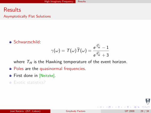
Schwarzschild:
γ(ω) = T (ω)T (ω) =eω
TH − 1
eω
TH + 3
where TH is the Hawking temperature of the event horizon.
Poles are the quasinormal frequencies.
First done in [Neitzke].
Exotic statistics?
Jose Natario (IST, Lisbon) Greybody Factors UP 2008 29 / 34
High Imaginary Frequency Results
ResultsAsymptotically Flat Solutions
Schwarzschild:
γ(ω) = T (ω)T (ω) =eω
TH − 1
eω
TH + 3
where TH is the Hawking temperature of the event horizon.
Poles are the quasinormal frequencies.
First done in [Neitzke].
Exotic statistics?
Jose Natario (IST, Lisbon) Greybody Factors UP 2008 29 / 34
High Imaginary Frequency Results
ResultsAsymptotically Flat Solutions
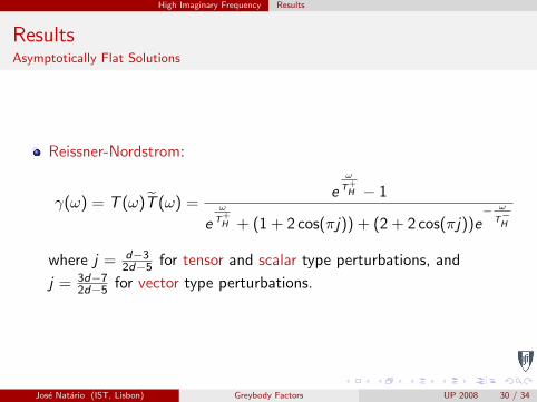
Reissner-Nordstrom:
γ(ω) = T (ω)T (ω) =eω
T+H − 1
eω
T+H + (1 + 2 cos(πj)) + (2 + 2 cos(πj))e
− ω
T−H
where j = d−32d−5 for tensor and scalar type perturbations, and
j = 3d−72d−5 for vector type perturbations.
Jose Natario (IST, Lisbon) Greybody Factors UP 2008 30 / 34

High Imaginary Frequency Results
ResultsAsymptotically de Sitter Solutions
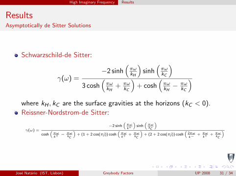
Schwarzschild-de Sitter:
γ(ω) =−2 sinh
(πωkH
)sinh
(πωkC
)3 cosh
(πωkH
+ πωkC
)+ cosh
(πωkH− πω
kC
)where kH , kC are the surface gravities at the horizons (kC < 0).
Reissner-Nordstrom-de Sitter:
γ(ω) =−2 sinh
“πωk+
”sinh
“πωkC
”cosh
“πωk+ − πω
kC
”+ (1 + 2 cos(πj)) cosh
“πωk+ + πω
kC
”+ (2 + 2 cos(πj)) cosh
“2πωk−
+ πωk+ + πω
kC
”
Jose Natario (IST, Lisbon) Greybody Factors UP 2008 31 / 34
High Imaginary Frequency Results
ResultsAsymptotically de Sitter Solutions
Schwarzschild-de Sitter:
γ(ω) =−2 sinh
(πωkH
)sinh
(πωkC
)3 cosh
(πωkH
+ πωkC
)+ cosh
(πωkH− πω
kC
)where kH , kC are the surface gravities at the horizons (kC < 0).
Reissner-Nordstrom-de Sitter:
γ(ω) =−2 sinh
“πωk+
”sinh
“πωkC
”cosh
“πωk+ − πω
kC
”+ (1 + 2 cos(πj)) cosh
“πωk+ + πω
kC
”+ (2 + 2 cos(πj)) cosh
“2πωk−
+ πωk+ + πω
kC
”
Jose Natario (IST, Lisbon) Greybody Factors UP 2008 31 / 34

High Imaginary Frequency Results
ResultsAsymptotically Anti de Sitter Solutions
Schwarzschild-Anti de Sitter: γ(ω) = 1.
Reissner-Nordstrom-Anti de Sitter: γ(ω) = 1.
In this case there are no poles because of reflecting boundaryconditions are imposed when computing quasinormal modes.
Jose Natario (IST, Lisbon) Greybody Factors UP 2008 32 / 34

Summary and Outlook
Summary and Outlook
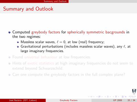
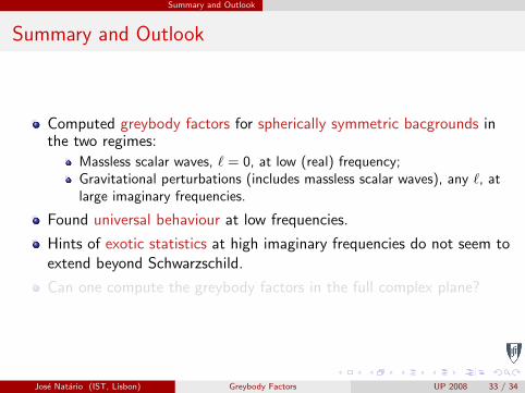
Computed greybody factors for spherically symmetric bacgrounds inthe two regimes:
Massless scalar waves, ` = 0, at low (real) frequency;Gravitational perturbations (includes massless scalar waves), any `, atlarge imaginary frequencies.
Found universal behaviour at low frequencies.
Hints of exotic statistics at high imaginary frequencies do not seem toextend beyond Schwarzschild.
Can one compute the greybody factors in the full complex plane?
Jose Natario (IST, Lisbon) Greybody Factors UP 2008 33 / 34

Summary and Outlook
Summary and Outlook
Computed greybody factors for spherically symmetric bacgrounds inthe two regimes:
Massless scalar waves, ` = 0, at low (real) frequency;Gravitational perturbations (includes massless scalar waves), any `, atlarge imaginary frequencies.
Found universal behaviour at low frequencies.
Hints of exotic statistics at high imaginary frequencies do not seem toextend beyond Schwarzschild.
Can one compute the greybody factors in the full complex plane?
Jose Natario (IST, Lisbon) Greybody Factors UP 2008 33 / 34
Summary and Outlook
Summary and Outlook
Computed greybody factors for spherically symmetric bacgrounds inthe two regimes:
Massless scalar waves, ` = 0, at low (real) frequency;Gravitational perturbations (includes massless scalar waves), any `, atlarge imaginary frequencies.
Found universal behaviour at low frequencies.
Hints of exotic statistics at high imaginary frequencies do not seem toextend beyond Schwarzschild.
Can one compute the greybody factors in the full complex plane?
Jose Natario (IST, Lisbon) Greybody Factors UP 2008 33 / 34

Summary and Outlook
Summary and Outlook
Computed greybody factors for spherically symmetric bacgrounds inthe two regimes:
Massless scalar waves, ` = 0, at low (real) frequency;Gravitational perturbations (includes massless scalar waves), any `, atlarge imaginary frequencies.
Found universal behaviour at low frequencies.
Hints of exotic statistics at high imaginary frequencies do not seem toextend beyond Schwarzschild.
Can one compute the greybody factors in the full complex plane?
Jose Natario (IST, Lisbon) Greybody Factors UP 2008 33 / 34
Summary and Outlook
Summary and Outlook
Computed greybody factors for spherically symmetric bacgrounds inthe two regimes:
Massless scalar waves, ` = 0, at low (real) frequency;Gravitational perturbations (includes massless scalar waves), any `, atlarge imaginary frequencies.
Found universal behaviour at low frequencies.
Hints of exotic statistics at high imaginary frequencies do not seem toextend beyond Schwarzschild.
Can one compute the greybody factors in the full complex plane?
Jose Natario (IST, Lisbon) Greybody Factors UP 2008 33 / 34
Appendix
Bibliography
Troels Harmark, JN and Ricardo Schiappa,Greybody Factors for d-Dimensional Black Holes,Advances in Theoretical and Mathematical Physics (in press),arXiv:0708.0017 [hep-th].
S. Das, G. Gibbons and S. Mathur,Universality of the Low Energy Absorption Cross-Sections for BlackHoles,Physical Review Letters 78 (1997) 417,arXiv:hep-th/9609052.
A. Neitzke,Greybody Factors at Large Imaginary Frequencies,arXiv:hep-th/0304080.
Jose Natario (IST, Lisbon) Greybody Factors UP 2008 34 / 34