Greenhouse Gas and Nitrogen Fertilizer Scenarios for U.S

Greenhouse Gas and Nitrogen Fertilizer Scenarios for U.S. Agriculture and Global Biofuels

Amani Elobeid, Miguel Carriquiry, Jacinto F. Fabiosa, Kranti Mulik, Dermot J. Hayes, Bruce A. Babcock, Jerome Dumortier, and Francisco Rosas

Working Paper 11-WP 524 June 2011

Center for Agricultural and Rural Development Iowa State University

Ames, Iowa 50011-1070 www.card.iastate.edu

Funding for this study came from the David and Lucile Packard Foundation. The authors thank the foundation for this support. This report is available online on the CARD Web site: www.card.iastate.edu. Permission is granted to excerpt or quote this information with appropriate attribution to the authors. Questions or comments about the contents of this paper should be directed to Jacinto Fabiosa, 568E Heady Hall, Iowa State University, Ames, Iowa 50011-1070; Ph: (515) 294-6183; E-mail: [email protected]. Iowa State University does not discriminate on the basis of race, color, age, religion, national origin, sexual orientation, gender identity, genetic information, sex, marital status, disability, or status as a U.S. veteran. Inquiries can be directed to the Director of Equal Opportunity and Compliance, 3280 Beardshear Hall, (515) 294-7612.

Abstract

This analysis uses the 2011 FAPRI-CARD (Food and Agricultural Policy Research

Institute–Center for Agricultural and Rural Development) baseline to evaluate the impact of four

alternative scenarios on U.S. and world agricultural markets, as well as on world fertilizer use

and world agricultural greenhouse gas emissions. A key assumption in the 2011 baseline is that

ethanol support policies disappear in 2012. The baseline also assumes that existing biofuel

mandates remain in place and are binding. Two of the scenarios are adverse supply shocks, the

first being a 10% increase in the price of nitrogen fertilizer in the United States, and the second, a

reversion of cropland into forestland. The third scenario examines how lower energy prices

would impact world agriculture. The fourth scenario reintroduces biofuel tax credits and duties.

Given that the baseline excludes these policies, the fourth scenario is an attempt to understand

the impact of these policies under the market conditions that prevail in early 2011. A key to

understanding the results of this fourth scenario is that in the absence of tax credits and duties,

the mandate drives biofuel use. Therefore, when the tax credits and duties are reintroduced, the

impacts are relatively small. In general, the results show that the entire international commodity

market system is remarkably robust with respect to policy changes in one country or in one

sector. The policy implication is that domestic policy changes implemented by a large

agricultural producer like the United States can have fairly significant impacts on the aggregate

world commodity markets. A second point that emerges from the results is that the law of

unintended consequences is at work in world agriculture. For example, a U.S. nitrogen tax that

might presumably be motivated for environmental benefit results in an increase in world

greenhouse gas emissions. A similar situation occurs in the afforestation scenario in which crop

production shifts from high-yielding land in the United States to low-yielding land and probably

native vegetation in the rest of the world, resulting in an unintended increase in global

greenhouse gas emissions.

Keywords: afforestation, energy price, ethanol tax credit, fertilizer, partial equilibrium model,

policy analysis.

1

1. Introduction

World agriculture has been significantly impacted by a number of events that have occurred in the past five years. Arguably the most prominent is the dramatic global expansion of biofuels, especially in the United States and Brazil, driven by mandates, federal and state incentives, and trade barriers. Energy prices have also increased to record levels, with the world crude oil price exceeding $130 per barrel in July of 2008 and currently hovering between $110 and $120 per barrel.1 Additionally, several major policy initiatives relating to climate change in general and biofuels in particular were initiated in a number of countries. These include such policies as the American Clean Energy and Security Act of 2009 in the United States and the 2009 Energy and Climate Change Package in the European Union (USDA, 2009; USDA, 2010). These events have changed the agricultural landscape in a number of ways. The primary feedstocks in biofuel production are currently agricultural crops, mainly corn for ethanol and soybeans for biodiesel. This means that there now exists a “new” direct link between agricultural and energy markets. While previously energy prices influenced agriculture primarily by impacting the cost of production, now energy prices directly influence the demand for crops used in biofuels, and consequently biofuel feedstock prices (Tokgoz et al., 2007; Hayes et al., 2009). This link between energy and agriculture becomes stronger as energy prices continue to rise and the agricultural feedstock becomes more competitive in the energy market. Conversely, agriculture now influences energy given the competition of the agricultural feedstock, through biofuels, in the energy sector (Muller et al., 2007). Du and Hayes (2011) found that, on average, the increase in ethanol production over the period 2000-2010 reduced wholesale gasoline prices by $0.25 per gallon. Continued support for increased biofuel production through mandates such as the Renewable Fuel Standard (RFS) is expected to strengthen these linkages. Climate change policy initiatives will also impact agriculture. These policies are supported by economic analyses pointing to land-use change as a major contributor in greenhouse gas (GHG) emissions impacts. For example, the California Air Resources Board (CARB) estimates GHG emissions from land-use change to account for 29% to 69% of total emissions. The U.S. Environmental Protection Agency’s RFS2 life-cycle analysis includes other sources of GHG emissions such as emissions from livestock production, use of farm inputs (e.g., fertilizer), and methane from rice, but GHG emissions from land-use change still account for 35% of total emissions. Agricultural changes in general and in land use in particular play a key role in determining the effectiveness of major policy proposals aimed at mitigating climate change, including the implementation of different offset policies that encourage afforestation. Brown et al. (2010) showed that carbon prices as low as $30 per metric ton provide enough of an incentive such that a significant amount of U.S. cropland would be used to grow trees, causing an increase

1 Data on the world crude oil price is from the U.S. Energy Information Administration (EIA 2011) (all countries spot price FOB weighted by estimated export volume).

2

in agricultural commodity prices in the United States and consequently impacting agriculture in other countries.

The overall purpose of this study is to provide policy-relevant information to further the development of rational policies aimed at mitigating negative environmental impacts of the agricultural and biofuels sectors.2 Specifically, the objective is to analyze the impact of four alternative scenarios: a U.S. fertilizer scenario, a low energy price scenario, a biofuel tax credit and duty scenario, and an afforestation scenario. An enhanced version of the deterministic FAPRI-CARD agricultural modeling system is used for this analysis.3 First a baseline is established and then the four scenarios are run. The impacts of these scenarios on the production, trade, and prices of agricultural commodities both in the United States and globally are measured in terms of their resulting departure from the baseline. The paper is organized into five sections. The next section describes the methodology, which includes a description of the model as well as the improvements made to the model in order to provide more accurate analyses of the scenarios. The third section provides an overview of the baseline projections. A description of the four scenarios and the results from these scenarios are presented in Section 4. The last section summarizes and concludes the paper.

2. Methodology Description of the FAPRI-CARD Modeling System The FAPRI-CARD agricultural modeling system is a set of multi-market, partial-equilibrium, and non-spatial econometric models.4 The models cover all major temperate crops, sugar, biofuels, dairy, and livestock and meat products for all major producing and consuming countries and are calibrated on the most recently available data (see Table 1). They have been used extensively for generating 10- to 15-year baseline projections for agricultural markets and for policy analysis based on the baseline projections. Data on supply and utilization for the commodities are obtained primarily from the United States Department of Agriculture (USDA) PSD Online and the Food and Agriculture Organization of the United Nations (FAO) FAOSTAT, and macroeconomic historical data and projections are obtained from the

2 The David and Lucile Packard Foundation provided funding to the Center for Agricultural and Rural Development (CARD) at Iowa State University to develop its modeling capability and to conduct this analysis. 3 FAPRI is the Food and Agricultural Policy Research Institute at Iowa State University. 4 We call the modeling system FAPRI-CARD to distinguish it from the FAPRI system, which involves a model of the U.S. agricultural sector developed and maintained by the University of Missouri at Columbia and international models developed and maintained at Iowa State University. In the FAPRI-CARD system, both the domestic and international models are maintained at Iowa State University.

3

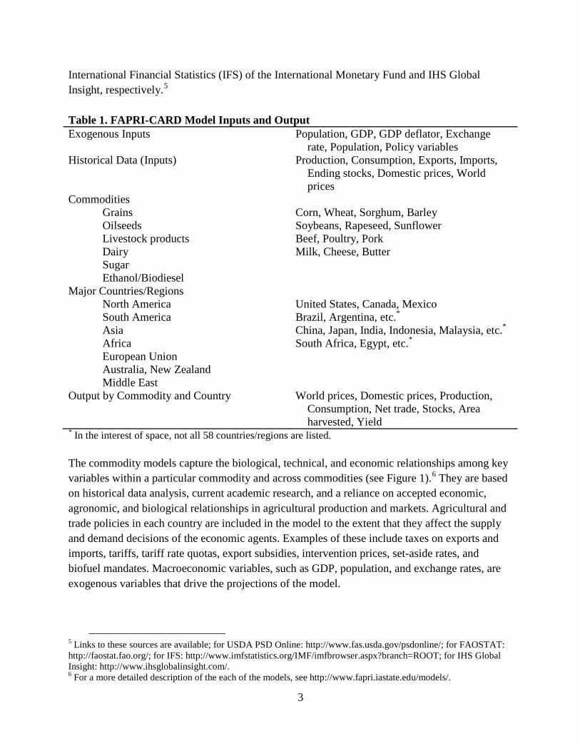
International Financial Statistics (IFS) of the International Monetary Fund and IHS Global Insight, respectively.5 Table 1. FAPRI-CARD Model Inputs and Output Exogenous Inputs Population, GDP, GDP deflator, Exchange

rate, Population, Policy variables Historical Data (Inputs) Production, Consumption, Exports, Imports,

Ending stocks, Domestic prices, World prices

Commodities Grains Corn, Wheat, Sorghum, Barley Oilseeds Soybeans, Rapeseed, Sunflower Livestock products Beef, Poultry, Pork Dairy Milk, Cheese, Butter Sugar Ethanol/Biodiesel Major Countries/Regions North America United States, Canada, Mexico South America Brazil, Argentina, etc.*

Asia China, Japan, India, Indonesia, Malaysia, etc.* Africa South Africa, Egypt, etc.* European Union Australia, New Zealand Middle East Output by Commodity and Country World prices, Domestic prices, Production,

Consumption, Net trade, Stocks, Area harvested, Yield

* In the interest of space, not all 58 countries/regions are listed. The commodity models capture the biological, technical, and economic relationships among key variables within a particular commodity and across commodities (see Figure 1).6 They are based on historical data analysis, current academic research, and a reliance on accepted economic, agronomic, and biological relationships in agricultural production and markets. Agricultural and trade policies in each country are included in the model to the extent that they affect the supply and demand decisions of the economic agents. Examples of these include taxes on exports and imports, tariffs, tariff rate quotas, export subsidies, intervention prices, set-aside rates, and biofuel mandates. Macroeconomic variables, such as GDP, population, and exchange rates, are exogenous variables that drive the projections of the model.

5 Links to these sources are available; for USDA PSD Online: http://www.fas.usda.gov/psdonline/; for FAOSTAT: http://faostat.fao.org/; for IFS: http://www.imfstatistics.org/IMF/imfbrowser.aspx?branch=ROOT; for IHS Global Insight: http://www.ihsglobalinsight.com/. 6 For a more detailed description of the each of the models, see http://www.fapri.iastate.edu/models/.

http://www.fas.usda.gov/psdonline/

http://faostat.fao.org/

http://www.imfstatistics.org/IMF/imfbrowser.aspx?branch=ROOT

4

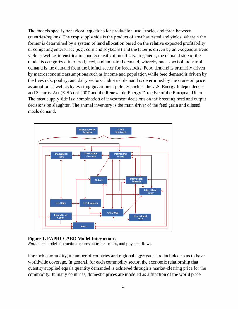
The models specify behavioral equations for production, use, stocks, and trade between countries/regions. The crop supply side is the product of area harvested and yields, wherein the former is determined by a system of land allocation based on the relative expected profitability of competing enterprises (e.g., corn and soybeans) and the latter is driven by an exogenous trend yield as well as intensification and extensification effects. In general, the demand side of the model is categorized into food, feed, and industrial demand, whereby one aspect of industrial demand is the demand from the biofuel sector for feedstocks. Food demand is primarily driven by macroeconomic assumptions such as income and population while feed demand is driven by the livestock, poultry, and dairy sectors. Industrial demand is determined by the crude oil price assumption as well as by existing government policies such as the U.S. Energy Independence and Security Act (EISA) of 2007 and the Renewable Energy Directive of the European Union. The meat supply side is a combination of investment decisions on the breeding herd and output decisions on slaughter. The animal inventory is the main driver of the feed grain and oilseed meals demand.

Figure 1. FAPRI-CARD Model Interactions Note: The model interactions represent trade, prices, and physical flows. For each commodity, a number of countries and regional aggregates are included so as to have worldwide coverage. In general, for each commodity sector, the economic relationship that quantity supplied equals quantity demanded is achieved through a market-clearing price for the commodity. In many countries, domestic prices are modeled as a function of the world price

5

using a price transmission equation, which includes exchange rates and relevant trade policies. As is evident from Figure 1, since econometric models for each sector can be linked, changes in one commodity sector will impact the other sectors. The models are run in Microsoft Excel. Generally the modeling system is comprised of commodity models with the exception of two country models, the United States and Brazil. The U.S. crops model is a partial-equilibrium model, which includes behavioral equations that determine crop planted acreage; domestic feed, food, and industrial uses; trade; and ending stocks in marketing years. The model solves for the set of prices that brings annual supply and demand into balance in all markets. The U.S. crops model is divided into nine regions, with area equations for each crop grown within each region. For crops with by-products, behavioral equations for the by-products are also included, for example high fructose corn syrup (HFCS), ethanol, and corn oil from corn, and soybean meal, soybean oil, and biodiesel from soybeans. For each commodity, a market-clearing price is calculated by equating quantity supplied to quantity demanded. Four important changes to the models have been recently implemented. These include a new yield specification in the crops models, the expansion of dried distillers’ grains with solubles (DDGS), and the development of a Brazilian regional model as well as a GHG accounting model. The yield equations were modified to be able to capture potential intensification and extensification impacts of prices. The intensification effect reflects more intensive use of inputs such as fertilizer when revenue grows faster than cost. The extensification effect reflects declining yield as more marginal land is brought into production. To complement the new yield intensification specification, we introduced a fertilizer component in which growth in yield from a purely intensification effect is associated with a change in the rate of nitrogen-phosphorous-potassium (N-P-K) fertilizer application per hectare. We also expanded the coverage of the DDGS model to include all countries covered by the FAPRI-CARD modeling system. The specification follows after the DDGS model specification in the U.S. module with some modification to address data constraints (FAPRI-MU, 2010). Additionally, a regionally disaggregated model of Brazilian agriculture was developed and integrated into the system. Because of its size and geographical location, Brazil encompasses widely varying ecosystems, ranging from grassland and crops associated with temperate climates in the South to tropical forests in the North and semiarid areas in the Northeast. The different regions also present enormous developmental disparities in terms of infrastructure, logistics, and strategies available to increase production. Thus, while rapid expansion of production of some commodities may only be achieved by taking area away from other agricultural activities in land-constrained regions, increases in area used by all activities may be observed in other parts of the country, which points to distinct dynamics in the competition for land across space. The six-region model also includes a second crop for corn, which is important in tracking land-use change to avoid double counting in their associated GHG emissions. Also, pastureland is directly

6

considered in the agricultural land allocation system, and the animal stocking rate is endogenously determined. Finally, a model that is able to account for the GHG emissions from agriculture, and that can be linked to the FAPRI-CARD system, is now in place. The model, called GreenAgSiM, estimates emissions according to the categories for national GHG inventories established by the Intergovernmental Panel on Climate Change. These categories include emissions from enteric fermentation and manure management from livestock, agricultural soil management, rice cultivation, and land-use change. GreenAgSiM consists of two components that use data from the FAPRI-CARD model as inputs. The first is the agricultural production component, which includes enteric fermentation, manure management, rice cultivation, and agricultural soil management. The second is the land-use change component, which captures emissions induced by land-use change occurring if forest and grassland are converted into cropland. Initially, this part relied on agricultural land as the major driver for land-use change and did not model the competition between forest, grassland, and agricultural land explicitly. As outlined in the model improvements, rules have been introduced to better track land-use change, including change in pasture and forests. With the data derived from FAPRI-CARD, the emissions from direct and indirect land-use change can be estimated. Model Improvements for this Study A number of model improvements are incorporated in this analysis to better capture land-use change, GHG emissions, and the effects of fertilizer use.

• To better capture differences in land quality, productivity, and climate considerations, we divided our regional aggregates into five regions, namely, Other Africa, Other America, Other Asia, Other Europe, and Other Oceania.

• We updated our trend yield parameter estimates to include new data for all crops and for all countries.

• We added a fertilizer component to the FAPRI-CARD model to better represent the effects of fertilizer on a crop’s output and GHG emissions, as well as to project fertilizer application rates and fertilizer demand on a global scale.

• The GHG accounting model was upgraded in two areas. It now uses the mentioned fertilizer application rates and aggregate fertilizer demand information from the FAPRI-CARD model. And we introduced rules to better characterize the land-use change associated with changes in cropland and pastureland from the FAPRI-CARD model.

• We introduced a cellulosic ethanol sector in the U.S. crops model that responds to economic incentives such as production subsidies and mandates.

Regarding the fertilizer component added to the model, changes in yields due to intensification are linked to changes in the fertilizer cost. The fertilizer cost is composed of the application rate

7

of nitrogen, phosphorous, and potassium multiplied by their respective prices. The linkage between yields and fertilizer cost is a function of the yield elasticities with respect to fertilizer application rates and the share of fertilizer cost in the total variable cost. This component also enables us to project fertilizer application rates and fertilizer demand by commodity, by country, and by nutrient. A more detailed explanation of the FAPRI-CARD fertilizer component is available in a paper by Rosas (2011). In terms of the GHG accounting model, the model was upgraded to better capture the GHG emissions from global agricultural production and land-use change. For example, because of the new fertilizer component that can now provide fertilizer use projections, GHG emissions from agricultural soil management can be better captured. A more substantial improvement in the model is a better tracking of changes in land use and their associated GHG emissions from changes in carbon from the biomass and soil. The model now tracks six categories of land, namely, forest, shrub land, grass land, set-aside, cropland, and pasture. Pastureland is derived from changes in animal inventory and some historical stocking rate. Cropland and pastureland are aggregated into one category—agricultural land. The algorithm of land dynamics in the model for increases in agricultural land is such that idle land comes into production first. Moreover, a “last in, first out” rule is applied in the conversion of agricultural land. Only when idle land is exhausted will native vegetation be converted into agricultural land. The respective shares in the land inventory are used to estimate how much of each native vegetation is converted. In case of decreases in agricultural land, reversion goes to idle land first. This reverted cropland is the first land that comes into production if more cropland is needed in a later period. A more detailed description of this model is given in a paper by Dumortier et al. (2010). The cellulosic ethanol module of the U.S. crops model is comprised of two markets: a cellulosic ethanol market, and a feedstock market. The cellulosic ethanol market is driven by ethanol demand in the retail market and at the gasoline blenders’ level, as well as by ethanol supply from ethanol plants. At the retail market, ethanol is a homogenous product regardless of its feedstock. That is, the same price is paid by consumers for blended gasoline whether ethanol is from corn, sugarcane, or cellulosic feedstock. However, at the blenders’ level, because of their specific RFS requirements, ethanol is differentiated such that the wholesale price of conventional, advanced, and cellulosic ethanol can vary. To supply ethanol in the ethanol market, ethanol plants become buyers for feedstocks in the feedstock market. In the cellulosic model, feedstock supplies currently come from corn stover and switchgrass. The demand for cellulosic ethanol by gasoline blenders is driven by net return of the blenders. In equilibrium, the prices for ethanol and feedstocks are jointly determined. The equilibrium prices are market-clearing prices that equate cellulosic ethanol demand and cellulosic ethanol supply and feedstock demand and feedstock supply.

8

3. Baseline Results Description of the Baseline The baseline provides a starting point for evaluating and comparing scenarios. This baseline gives 15-year projections (2011-2025) of world agricultural production, consumption, stocks, trade, and prices by country and commodity.7 The projections are grounded in a series of assumptions about the general economy, agricultural policies, the weather, and technological change. Specifically, these projections are based on the assumption of average weather patterns, existing farm policy, and policy commitments under current trade agreements and custom unions. They also generally assume that current agricultural policies will remain in force in the United States and in other trading nations during the projection period. Bioenergy mandates in a number of countries are key drivers in the baseline. In the United States, the Renewable Fuel Standard (RFS) and other provisions of the EISA 2007 are implemented, with the exception of the cellulosic ethanol RFS (because of waivers). The existing U.S. biofuel mandates are binding in the baseline. Another key assumption is that ethanol and biodiesel support policies in the United States disappear in 2012. These include ethanol and biodiesel tax credits and biofuel import tariffs. In addition, the Food, Conservation, and Energy Act (FCEA) of 2008 in the United States and the current provisions of the Common Agricultural Policy in the European Union are included in the baseline. The commitments of contracting countries in the Uruguay Round Agreements Act of 1995 are extended to 2025. Additionally, long-run equilibrium is imposed in the ethanol sector in the United States as well as in the international livestock and dairy sectors. In the long run, in equilibrium, there is no incentive to build new ethanol plants and there is no incentive to shut down existing plants. This means that the profit margins of the ethanol plants are zero in the long run. In the livestock and dairy sectors, supply and prices adjust so that net returns go back to “normal” levels in the long run; that is, the returns are at levels sufficient to keep producers in business. This long-run equilibrium is imposed in the year 2023.8 Macroeconomic Environment The baseline projections are run against a backdrop of a macroeconomic environment that includes an economic turnaround, which began in 2010, continuing population growth and urbanization, and ever-expanding biofuel mandates such as the EISA 2007 in the United States

7 In marketing years, 2011 represents 2011/12. All crops are in marketing years while biofuels, livestock, and dairy are in calendar years. 8 Although the projections extend to 2025, we impose the long-run equilibrium in 2023 to allow the models an additional couple of years to adjust.

9

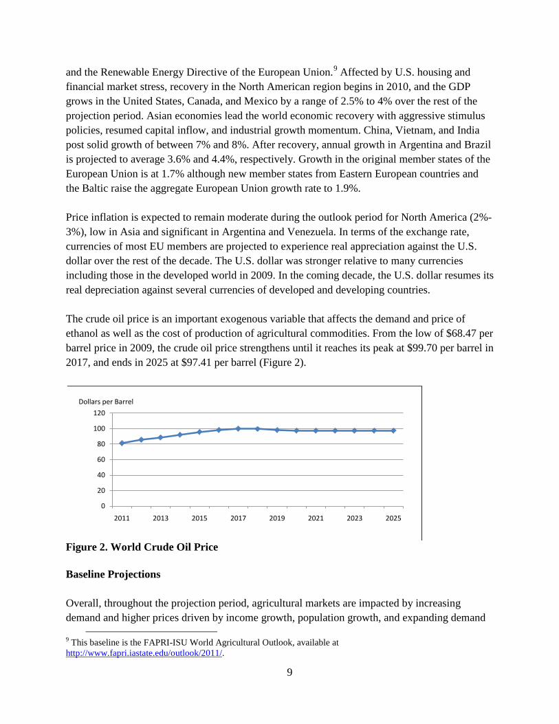
and the Renewable Energy Directive of the European Union.9 Affected by U.S. housing and financial market stress, recovery in the North American region begins in 2010, and the GDP grows in the United States, Canada, and Mexico by a range of 2.5% to 4% over the rest of the projection period. Asian economies lead the world economic recovery with aggressive stimulus policies, resumed capital inflow, and industrial growth momentum. China, Vietnam, and India post solid growth of between 7% and 8%. After recovery, annual growth in Argentina and Brazil is projected to average 3.6% and 4.4%, respectively. Growth in the original member states of the European Union is at 1.7% although new member states from Eastern European countries and the Baltic raise the aggregate European Union growth rate to 1.9%. Price inflation is expected to remain moderate during the outlook period for North America (2%-3%), low in Asia and significant in Argentina and Venezuela. In terms of the exchange rate, currencies of most EU members are projected to experience real appreciation against the U.S. dollar over the rest of the decade. The U.S. dollar was stronger relative to many currencies including those in the developed world in 2009. In the coming decade, the U.S. dollar resumes its real depreciation against several currencies of developed and developing countries. The crude oil price is an important exogenous variable that affects the demand and price of ethanol as well as the cost of production of agricultural commodities. From the low of $68.47 per barrel price in 2009, the crude oil price strengthens until it reaches its peak at $99.70 per barrel in 2017, and ends in 2025 at $97.41 per barrel (Figure 2).

Figure 2. World Crude Oil Price Baseline Projections Overall, throughout the projection period, agricultural markets are impacted by increasing demand and higher prices driven by income growth, population growth, and expanding demand

9 This baseline is the FAPRI-ISU World Agricultural Outlook, available at http://www.fapri.iastate.edu/outlook/2011/.

0

20

40

60

80

100

120

2011 2013 2015 2017 2019 2021 2023 2025

Dollars per Barrel

http://www.fapri.iastate.edu/outlook/2011/

10

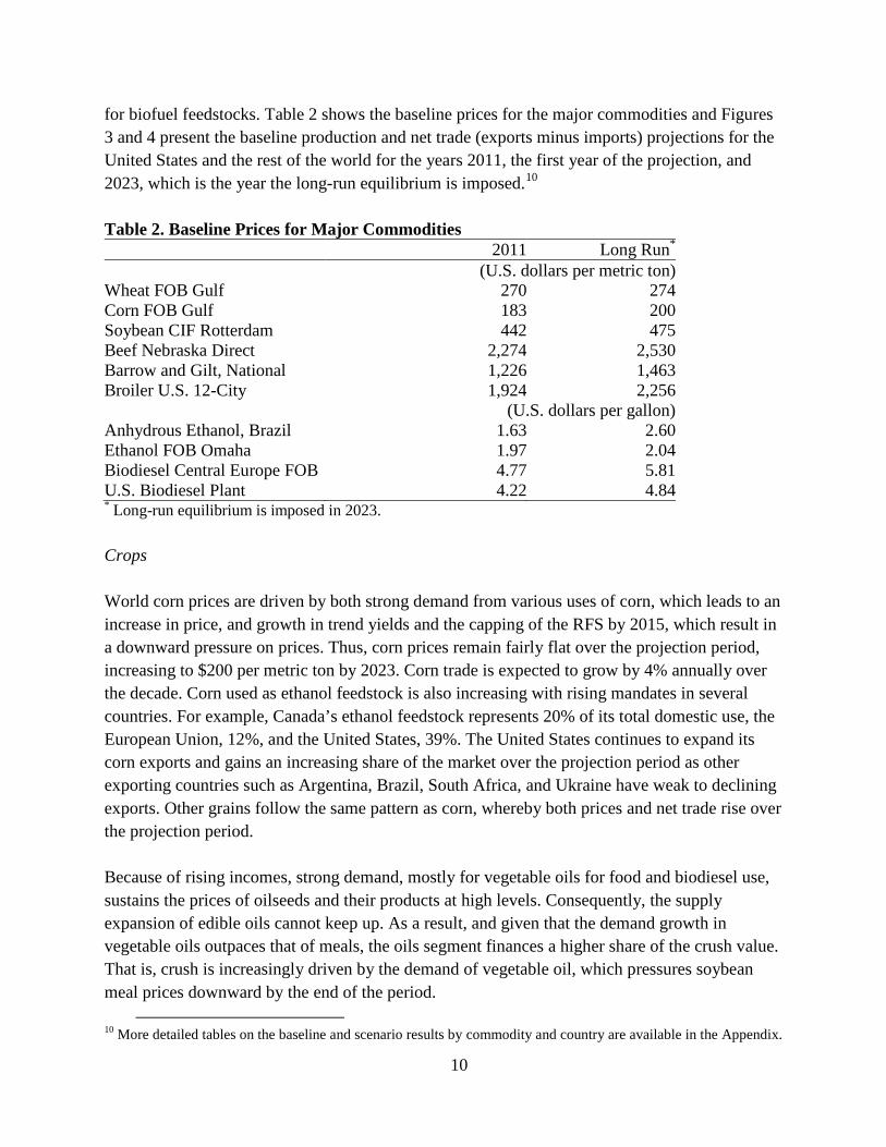
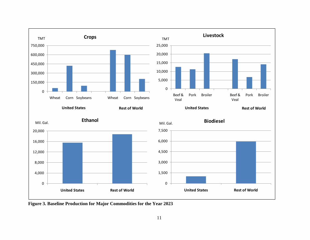
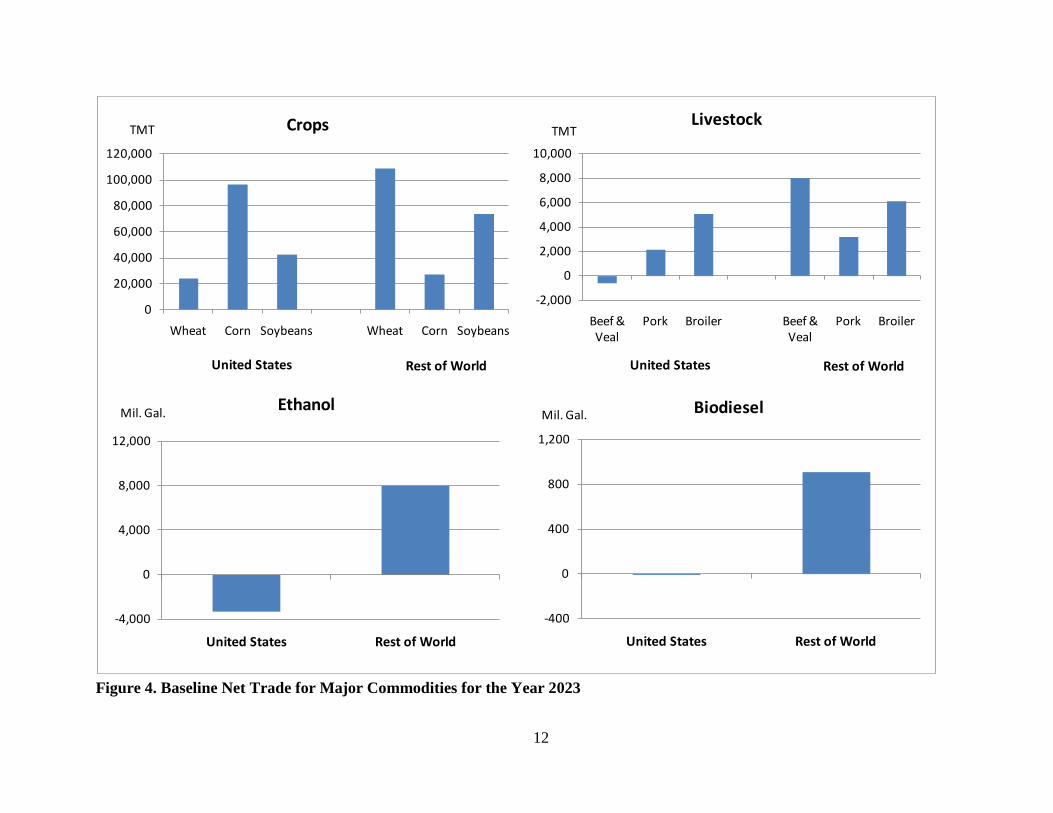
for biofuel feedstocks. Table 2 shows the baseline prices for the major commodities and Figures 3 and 4 present the baseline production and net trade (exports minus imports) projections for the United States and the rest of the world for the years 2011, the first year of the projection, and 2023, which is the year the long-run equilibrium is imposed.10 Table 2. Baseline Prices for Major Commodities

2011 Long Run*

(U.S. dollars per metric ton)

Wheat FOB Gulf 270 274 Corn FOB Gulf 183 200 Soybean CIF Rotterdam 442 475 Beef Nebraska Direct 2,274 2,530 Barrow and Gilt, National 1,226 1,463 Broiler U.S. 12-City 1,924 2,256

(U.S. dollars per gallon)

Anhydrous Ethanol, Brazil 1.63 2.60 Ethanol FOB Omaha 1.97 2.04 Biodiesel Central Europe FOB 4.77 5.81 U.S. Biodiesel Plant 4.22 4.84 * Long-run equilibrium is imposed in 2023. Crops World corn prices are driven by both strong demand from various uses of corn, which leads to an increase in price, and growth in trend yields and the capping of the RFS by 2015, which result in a downward pressure on prices. Thus, corn prices remain fairly flat over the projection period, increasing to $200 per metric ton by 2023. Corn trade is expected to grow by 4% annually over the decade. Corn used as ethanol feedstock is also increasing with rising mandates in several countries. For example, Canada’s ethanol feedstock represents 20% of its total domestic use, the European Union, 12%, and the United States, 39%. The United States continues to expand its corn exports and gains an increasing share of the market over the projection period as other exporting countries such as Argentina, Brazil, South Africa, and Ukraine have weak to declining exports. Other grains follow the same pattern as corn, whereby both prices and net trade rise over the projection period. Because of rising incomes, strong demand, mostly for vegetable oils for food and biodiesel use, sustains the prices of oilseeds and their products at high levels. Consequently, the supply expansion of edible oils cannot keep up. As a result, and given that the demand growth in vegetable oils outpaces that of meals, the oils segment finances a higher share of the crush value. That is, crush is increasingly driven by the demand of vegetable oil, which pressures soybean meal prices downward by the end of the period.

10 More detailed tables on the baseline and scenario results by commodity and country are available in the Appendix.

11

Figure 3. Baseline Production for Major Commodities for the Year 2023

0

150,000

300,000

450,000

600,000

750,000

Wheat Corn Soybeans Wheat Corn Soybeans

TMT Crops

United States Rest of World

0

5,000

10,000

15,000

20,000

25,000

Beef & Veal

Pork Broiler Beef & Veal

Pork Broiler

TMTLivestock


0

4,000

8,000

12,000

16,000

20,000


Mil. Gal. Ethanol

0

1,500

3,000

4,500

6,000

7,500


Mil. Gal. Biodiesel

12

Figure 4. Baseline Net Trade for Major Commodities for the Year 2023

0

20,000

40,000

60,000

80,000

100,000

120,000


TMT Crops


-2,000

0

2,000

4,000

6,000

8,000

10,000

Beef & Veal


Pork Broiler

TMTLivestock


-4,000

0

4,000

8,000

12,000


Mil. Gal. Ethanol

-400

0

400

800

1,200


Mil. Gal. Biodiesel

13

Livestock and Dairy Strong demand from growing incomes boosts world demand for livestock and dairy products and strengthens prices. Per capita meat consumption increases, with much of the growth in consumption occurring in countries and regions with limited productive potential for meat production. This increase in demand translates into higher trade, which grows at a rate of 2.9%. Coupled with the higher feed prices, prices of meat products remain strong over the projection period. To meet this growing demand, meat production also increases. On the supply side, Australia and Brazil gain the most market share in the beef market, while the United States gains the most in the pork and poultry markets. Biofuels With increasing demand to meet the RFS mandates, U.S. net imports increase over the projection period, reaching 3.3 billion gallons by 2023. U.S. ethanol production is also projected to increase, with ethanol production from corn totaling 15 billion gallons by 2023, utilizing 5 billion bushels of corn. Even at a crude oil price approaching $100 per barrel and the gasoline retail price at $3.25 per gallon with an associated ethanol retail price of $2.25 per gallon, the ethanol sector still does not exceed the RFS because of the high corn price. As a result, RIN (Renewable Identification Number) values are non-zero to compensate ethanol producers for any losses at the market demand price. The world price of biodiesel (Central Europe FOB) increases throughout the projection period, driven by higher petroleum prices, the demand expansion by growing domestic mandates in several countries (Brazil, Argentina, the European Union, and the United States), and higher vegetable oil prices. Consumption of biodiesel in the United States increases in 2011 as a result of implementation of the RFS. While production also increases, it is not enough to meet domestic needs. Therefore, the United States is expected to reverse its trade position and become a small net importer in 2011. Production increases throughout the outlook, but the country remains a net importer until the last few years of the period, in which it exports marginal quantities. Fertilizer World fertilizer use is projected to increase 5% by 2023 relative to the 2010 crop season, reflecting the expansion of the world’s cropland. Higher use is also driven by the more intensive use of fertilizers at the world level in commodities such as corn, barley, rapeseed, peanuts, and cotton, driven by their strong prices. World fertilizer use in corn is projected to be higher in NPK relative to 2010 because of the increase in both corn harvested areas and fertilizer application rates. This is especially true for the United States, the world’s second largest fertilizer consuming

14

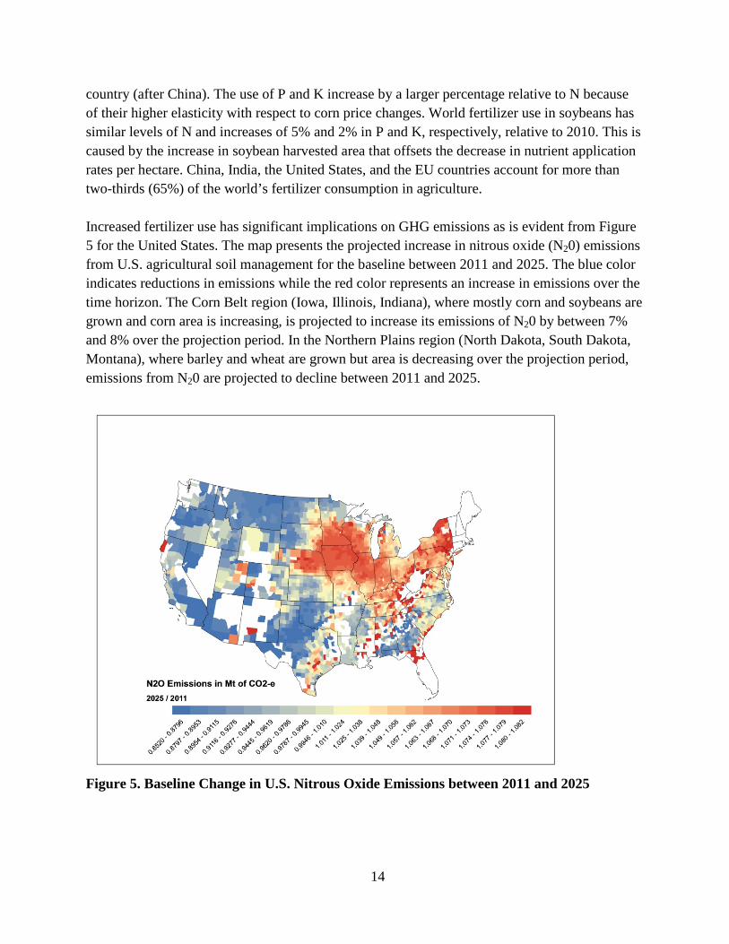
country (after China). The use of P and K increase by a larger percentage relative to N because of their higher elasticity with respect to corn price changes. World fertilizer use in soybeans has similar levels of N and increases of 5% and 2% in P and K, respectively, relative to 2010. This is caused by the increase in soybean harvested area that offsets the decrease in nutrient application rates per hectare. China, India, the United States, and the EU countries account for more than two-thirds (65%) of the world’s fertilizer consumption in agriculture. Increased fertilizer use has significant implications on GHG emissions as is evident from Figure 5 for the United States. The map presents the projected increase in nitrous oxide (N20) emissions from U.S. agricultural soil management for the baseline between 2011 and 2025. The blue color indicates reductions in emissions while the red color represents an increase in emissions over the time horizon. The Corn Belt region (Iowa, Illinois, Indiana), where mostly corn and soybeans are grown and corn area is increasing, is projected to increase its emissions of N20 by between 7% and 8% over the projection period. In the Northern Plains region (North Dakota, South Dakota, Montana), where barley and wheat are grown but area is decreasing over the projection period, emissions from N20 are projected to decline between 2011 and 2025.

Figure 5. Baseline Change in U.S. Nitrous Oxide Emissions between 2011 and 2025

15

Greenhouse Gas The expansion in crop area as well as the rise in meat demand and the resulting expansion in livestock increases emissions from livestock products (especially enteric fermentation) and puts pressure on global forests and grasslands. We estimate that global emissions from agricultural production rise by 14% over the projection period. A GHG emission efficiency (GHGee) is estimated that summarizes information about market outcome, productivity improvement, and GHG emissions into a single metric for a particular country in terms of aggregate value of agricultural production per ton of GHG emission. The average price over the projection period is the value aggregator for all the commodities produced in a given country, and emissions from agricultural production are considered. Higher GHGee values suggest a more efficient GHG emission performance. That is, a country is able to produce more value of agricultural production for every GHG that is emitted in the atmosphere. GHGee estimates for selected countries in 2010 show a wide differential between countries, with the European Union and the United States having a high value of agricultural production per ton of CO2-equivalent emitted at $579 and $571, respectively. This is followed by Argentina at $349, India at $329, China at $324, and Brazil at $212. Productivity improvement enables these countries to gain a 9% to 21% increase in their GHGee over the projection period.

4. Scenario Results Description of the Scenarios Once the baseline is established, specific scenarios are run and the results are compared with the baseline. The first scenario is a fertilizer scenario in which the price of nitrogen in the United States is increased by 10% over the baseline beginning in 2011 and extending to the final projection year of 2025. The second scenario, which is a low energy price scenario, involves the fixing of the crude oil price at $75/barrel from 2011 to 2025. This amounts to a 20% decline in the crude oil price on average relative to the baseline. Using an estimated regression relating the natural gas price to the crude oil price, we also reduce natural gas prices by 10%. The FAPRI-CARD U.S. cost of production model is run to reduce fertilizer prices in line with energy costs. The associated reduction in production costs is allowed to propagate to the rest of the world.

In the third scenario, the tax credit and duty scenario, the biofuel tax credit is reintroduced at $0.55/gallon for ethanol and at $1.00/gallon for biodiesel beginning in 2012 and continuing to 2025. We also re-impose during the same period the specific duty for ethanol of $0.54/gallon and the 2.5% ad valorem duty.

16

Finally, a U.S. afforestation scenario is analyzed in which we use the crop area displacement from afforestation used in a report by the Environmental Protection Agency (EPA, 2005). This amounted to 50 million acres of cropland displaced from production in the United States by 2025. This reduction is equivalent to a 15% decrease in the total cropland used for the 13 major crops, hay, and Conservation Reserve Program. The four scenarios are presented relative to the baseline projections by comparing the long-run equilibrium results for the baseline (year 2023) to those of the scenarios. The impacts on U.S. and world crops and livestock (i.e., agricultural markets), biofuels, and fertilizer are expressed in terms of percent change between the 2023 baseline and scenario numbers. The only exception is the impacts on GHG emissions, which are presented in terms of the average percent change over the projection period. Emissions, particularly for land-use change, are non-linear and vary significantly from year to year. Thus, average changes over the projection period tend to be more informative than choosing one particular year. Fertilizer Scenario Impact on Agricultural Markets We analyzed a fertilizer scenario in which the price of nitrogen in the United States is increased by 10% over the baseline from 2011 to 2025. U.S. farmers usually apply more nitrogen than they need in a typical year. They do this because they realize that nitrogen can leach in wet years and that it therefore makes economic sense to apply excess nitrogen to insure against wet spring weather. That is, when nitrogen fertilizer is inexpensive relative to its value when it is needed, farmers will apply more fertilizer than is needed in an average year. This is important because recent research suggests that nitrous oxide (N2O) emissions increase dramatically when nitrogen fertilizer rates exceed agronomic rates. To put the magnitude of this shock in perspective, total fertilizer cost accounts for almost 40% of corn total variable cost in the U.S. Corn Belt region, and the cost of nitrogen fertilizer represents about 50% of total fertilizer cost. In soybeans, total fertilizer cost accounts for 28% of total variable cost, and the cost of nitrogen fertilizer represents 9% of total fertilizer cost. Therefore, a 10% increase in the price of nitrogen fertilizer translates into an increase in variable costs in the Corn Belt of the order of roughly 2% and 0.25% for corn and soybeans, respectively. The change in the total variable cost directly affects both the area allocation and yield equations. Although the impacts are small, as expected, some interesting results emerge. As illustrated in the case of corn and soybeans, there will be some differential in the impacts across different crops because of the different intensity of the use of fertilizer, nitrogen fertilizer in particular. Additionally, since this is a shock only in the United States, there are offsetting effects when the response of the rest of the world is considered.

17

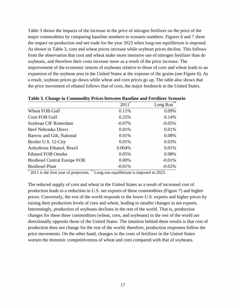
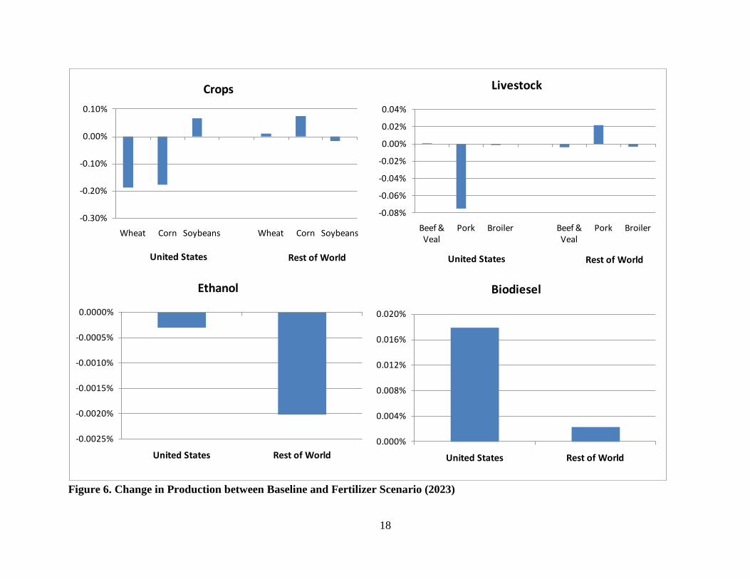
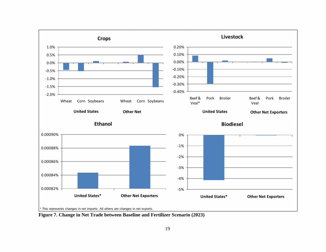
Table 3 shows the impacts of the increase in the price of nitrogen fertilizer on the price of the major commodities by comparing baseline numbers to scenario numbers. Figures 6 and 7 show the impact on production and net trade for the year 2023 when long-run equilibrium is imposed. As shown in Table 3, corn and wheat prices increase while soybean prices decline. This follows from the observation that corn and wheat make more intensive use of nitrogen fertilizer than do soybeans, and therefore their costs increase more as a result of the price increase. The improvement of the economic returns of soybeans relative to those of corn and wheat leads to an expansion of the soybean area in the United States at the expense of the grains (see Figure 6). As a result, soybean prices go down while wheat and corn prices go up. The table also shows that the price movement of ethanol follows that of corn, the major feedstock in the United States. Table 3. Change in Commodity Prices between Baseline and Fertilizer Scenario

2011* Long Run** Wheat FOB Gulf 0.11% 0.09% Corn FOB Gulf 0.25% 0.14% Soybean CIF Rotterdam -0.07% -0.05% Beef Nebraska Direct 0.01% 0.01% Barrow and Gilt, National 0.01% 0.08% Broiler U.S. 12-City 0.01% 0.03% Anhydrous Ethanol, Brazil 0.004% 0.01% Ethanol FOB Omaha 0.05% 0.08% Biodiesel Central Europe FOB 0.00% -0.01% Biodiesel Plant -0.01% -0.02% * 2011 is the first year of projection. ** Long-run equilibrium is imposed in 2023. The reduced supply of corn and wheat in the United States as a result of increased cost of production leads to a reduction in U.S. net exports of these commodities (Figure 7) and higher prices. Conversely, the rest of the world responds to the lower U.S. exports and higher prices by raising their production levels of corn and wheat, leading to smaller changes in net exports. Interestingly, production of soybeans declines in the rest of the world. That is, production changes for these three commodities (wheat, corn, and soybeans) in the rest of the world are directionally opposite those of the United States. The intuition behind these results is that cost of production does not change for the rest of the world; therefore, production responses follow the price movements. On the other hand, changes in the costs of fertilizer in the United States worsen the domestic competitiveness of wheat and corn compared with that of soybeans.

18

Figure 6. Change in Production between Baseline and Fertilizer Scenario (2023)

-0.30%

-0.20%

-0.10%

0.00%

0.10%


Crops


-0.08%

-0.06%

-0.04%

-0.02%

0.00%

0.02%

0.04%

Beef & Veal


Pork Broiler

Livestock


-0.0025%

-0.0020%

-0.0015%

-0.0010%

-0.0005%

0.0000%


Ethanol

0.000%

0.004%

0.008%

0.012%

0.016%

0.020%


Biodiesel

19

Figure 7. Change in Net Trade between Baseline and Fertilizer Scenario (2023)* This represents changes in net imports. All others are changes in net exports.

-2.0%

-1.5%

-1.0%

-0.5%

0.0%

0.5%

1.0%


Crops

United States Other Net

-0.40%

-0.30%

-0.20%

-0.10%

0.00%

0.10%

0.20%

Beef & Veal*


Pork Broiler

Livestock

United States Other Net Exporters

0.00082%

0.00084%

0.00086%

0.00088%

0.00090%

United States* Other Net Exporters

Ethanol

-5%

-4%

-3%

-2%

-1%

0%


Biodiesel

20

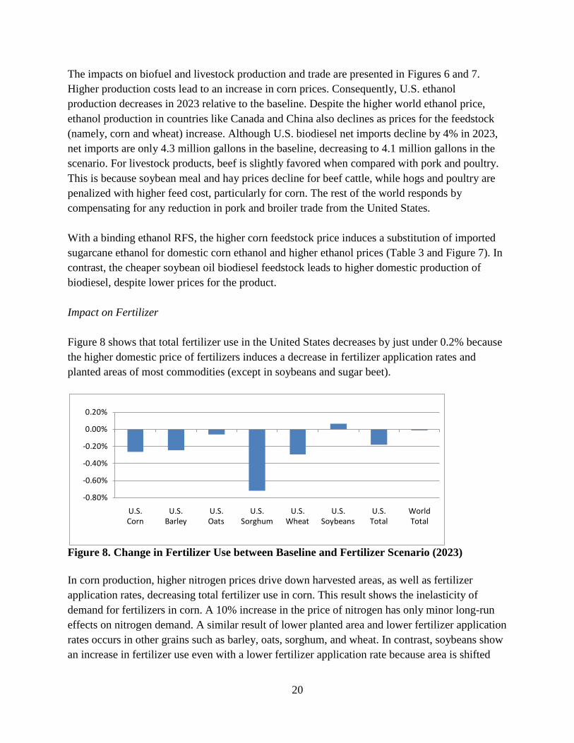
The impacts on biofuel and livestock production and trade are presented in Figures 6 and 7. Higher production costs lead to an increase in corn prices. Consequently, U.S. ethanol production decreases in 2023 relative to the baseline. Despite the higher world ethanol price, ethanol production in countries like Canada and China also declines as prices for the feedstock (namely, corn and wheat) increase. Although U.S. biodiesel net imports decline by 4% in 2023, net imports are only 4.3 million gallons in the baseline, decreasing to 4.1 million gallons in the scenario. For livestock products, beef is slightly favored when compared with pork and poultry. This is because soybean meal and hay prices decline for beef cattle, while hogs and poultry are penalized with higher feed cost, particularly for corn. The rest of the world responds by compensating for any reduction in pork and broiler trade from the United States. With a binding ethanol RFS, the higher corn feedstock price induces a substitution of imported sugarcane ethanol for domestic corn ethanol and higher ethanol prices (Table 3 and Figure 7). In contrast, the cheaper soybean oil biodiesel feedstock leads to higher domestic production of biodiesel, despite lower prices for the product. Impact on Fertilizer Figure 8 shows that total fertilizer use in the United States decreases by just under 0.2% because the higher domestic price of fertilizers induces a decrease in fertilizer application rates and planted areas of most commodities (except in soybeans and sugar beet).

Figure 8. Change in Fertilizer Use between Baseline and Fertilizer Scenario (2023) In corn production, higher nitrogen prices drive down harvested areas, as well as fertilizer application rates, decreasing total fertilizer use in corn. This result shows the inelasticity of demand for fertilizers in corn. A 10% increase in the price of nitrogen has only minor long-run effects on nitrogen demand. A similar result of lower planted area and lower fertilizer application rates occurs in other grains such as barley, oats, sorghum, and wheat. In contrast, soybeans show an increase in fertilizer use even with a lower fertilizer application rate because area is shifted

-0.80%

-0.60%

-0.40%

-0.20%

0.00%

0.20%

U.S. Corn

U.S. Barley

U.S. Oats

U.S. Sorghum

U.S. Wheat

U.S. Soybeans

U.S. Total

World Total

21

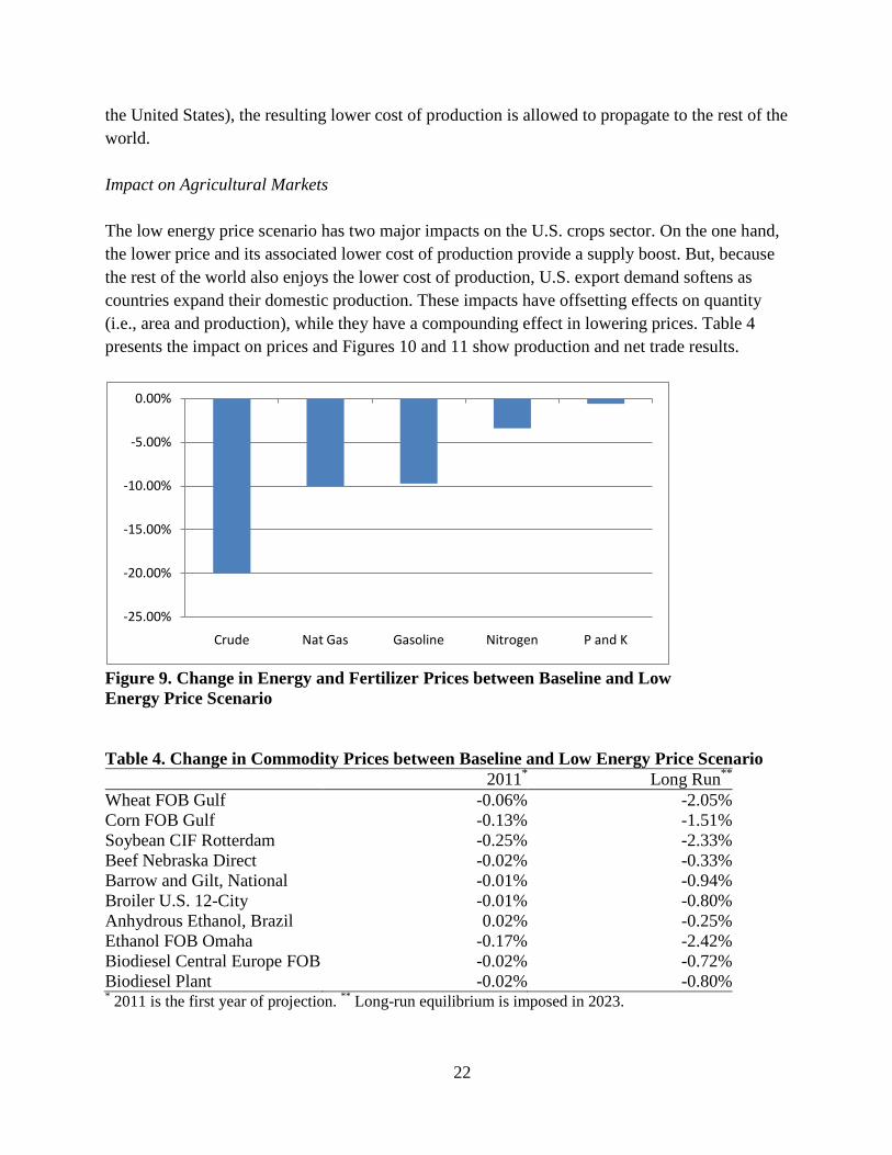
from nitrogen-intensive crops. Soybean production is characterized by a low use of nitrogen fertilizers because of the crop’s ability to fix nitrogen in soils from other sources, so an increase in the price of nitrogen is expected to make soybean production relatively more attractive. Since the nitrogen fertilizer price increase is isolated to the United States, the rest of the world responds to the higher world crop prices by increasing area and rates of fertilizer use, but the impacts are small. The overall consequence of such a policy is that the reduction in demand from U.S. nitrogen-intensive crops such as corn, barley, oats, and wheat is partially offset by the higher use in the rest of the world such that world fertilizer use shows only a minor reduction. Impact on Greenhouse Gas In terms of livestock and associated emissions, with the lower prices of soybean meal and hay offsetting the increase in the price of corn, there are no significant changes in GHG emissions from enteric fermentation and manure management. The more interesting aspect of the scenario is the inability of the 10% price increase to significantly reduce synthetic fertilizer emissions (nitrogen) in the United States. Over the projection period, emissions in the United States go down by an average of only 0.15% and also on a global scale, the reductions are negligible.11 An explanation for this phenomenon can be found in the fairly inelastic demand for nitrogen fertilizer in the United States. The scenario restricts the effects of the fertilizer price increase to the United States. That is, there is no transmission of the higher nitrogen fertilizer price in the United States to the price in the rest of the world. Area in the United States goes down by 0.07% on average, leading other countries to compensate for the reduced production by increasing their area. However, the increase in global crop area is small and leads to only slightly higher emissions when compared with the baseline. Carbon savings from land reversion in the United States may not be significant because reverted cropland goes into idle cropland category. However, land conversion in the rest of the world may be from native vegetation rich with sequestered carbon. The two main drivers of those emissions are India and China, both having low available idle land and a greater likelihood of conversion of native vegetation to supply increases in cropland. Low Energy Price Scenario For this scenario, the crude oil price is reduced by 20% on average relative to the baseline and is fixed at $75/barrel. The natural gas price is also decreased by 10% (Figure 9). Also, updated costs of production consistent with the lower energy prices assumed for this scenario were included.12 In contrast to the previous scenario (an increase in the price of nitrogen fertilizer in

11 Unlike the other impacts, which are expressed in terms of percent change between the baseline and the scenario for the year 2023, the impacts on GHG emissions are for the annual percent changes between the baseline and the scenario averaged over the projection period 2011-2023. 12 These new costs were calculated using the FAPRI-CARD U.S. cost of production model.

22

the United States), the resulting lower cost of production is allowed to propagate to the rest of the world. Impact on Agricultural Markets The low energy price scenario has two major impacts on the U.S. crops sector. On the one hand, the lower price and its associated lower cost of production provide a supply boost. But, because the rest of the world also enjoys the lower cost of production, U.S. export demand softens as countries expand their domestic production. These impacts have offsetting effects on quantity (i.e., area and production), while they have a compounding effect in lowering prices. Table 4 presents the impact on prices and Figures 10 and 11 show production and net trade results.

Figure 9. Change in Energy and Fertilizer Prices between Baseline and Low Energy Price Scenario Table 4. Change in Commodity Prices between Baseline and Low Energy Price Scenario

2011* Long Run** Wheat FOB Gulf -0.06% -2.05% Corn FOB Gulf -0.13% -1.51% Soybean CIF Rotterdam -0.25% -2.33% Beef Nebraska Direct -0.02% -0.33% Barrow and Gilt, National -0.01% -0.94% Broiler U.S. 12-City -0.01% -0.80% Anhydrous Ethanol, Brazil 0.02% -0.25% Ethanol FOB Omaha -0.17% -2.42% Biodiesel Central Europe FOB -0.02% -0.72% Biodiesel Plant -0.02% -0.80% * 2011 is the first year of projection. ** Long-run equilibrium is imposed in 2023.

-25.00%

-20.00%

-15.00%

-10.00%

-5.00%

0.00%

Crude Nat Gas Gasoline Nitrogen P and K

23

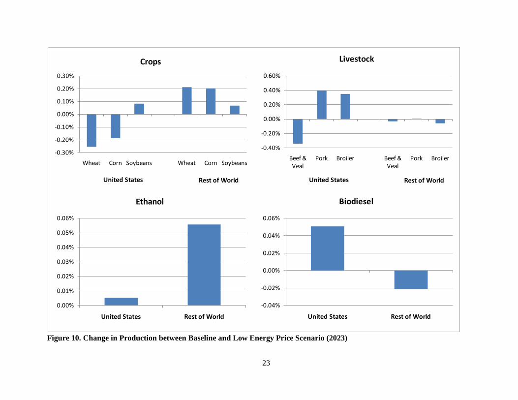
Figure 10. Change in Production between Baseline and Low Energy Price Scenario (2023)

-0.30%

-0.20%

-0.10%

0.00%

0.10%

0.20%

0.30%


Crops


-0.40%

-0.20%

0.00%

0.20%

0.40%

0.60%

Beef & Veal


Pork Broiler

Livestock


0.00%

0.01%

0.02%

0.03%

0.04%

0.05%

0.06%


Ethanol

-0.04%

-0.02%

0.00%

0.02%

0.04%

0.06%


Biodiesel

24

Figure 11. Change in Net Trade between Baseline and Low Energy Price Scenario (2023)* This represents changes in net imports. All others are changes in net exports.

-2.0%

-1.0%

0.0%

1.0%

2.0%


Crops


-2%

0%

2%

4%

6%

Beef & Veal*


Pork Broiler

Livestock


-0.030%

-0.020%

-0.010%

0.000%


Ethanol

-16%

-12%

-8%

-4%

0%


Biodiesel

25

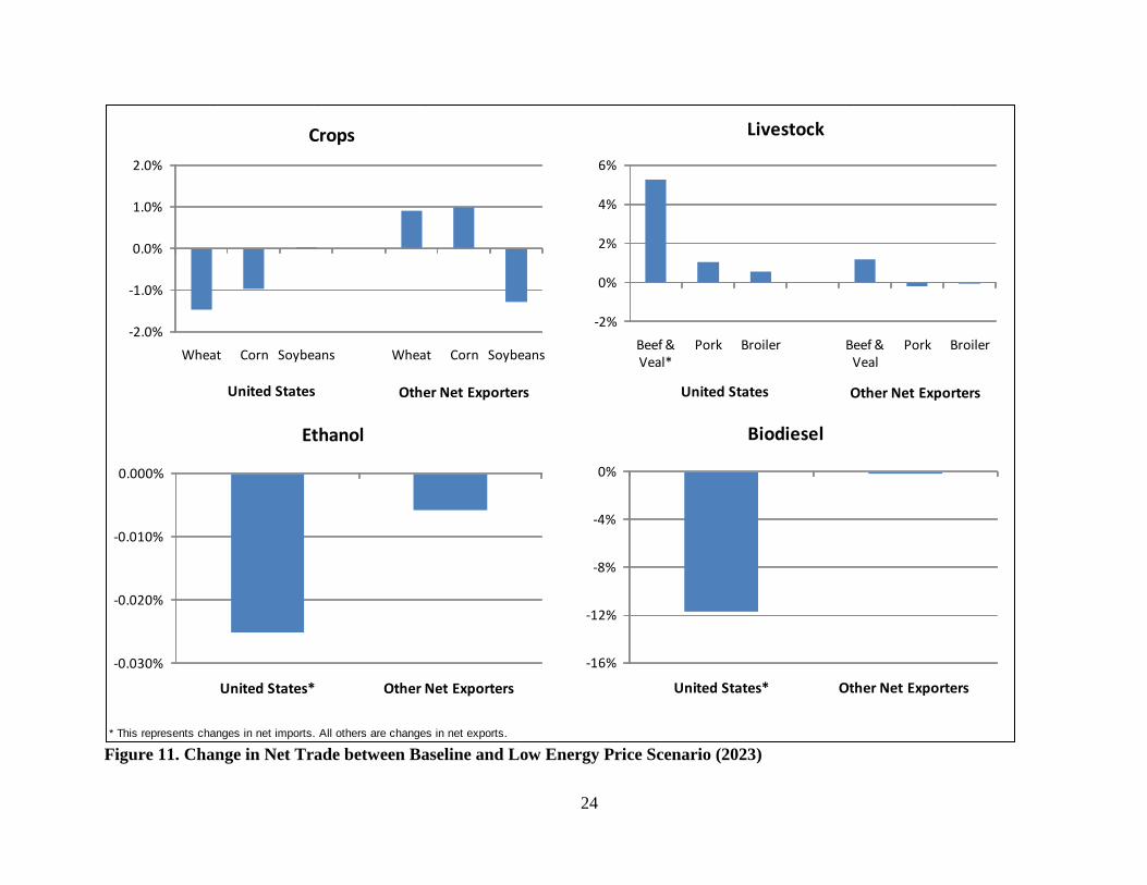
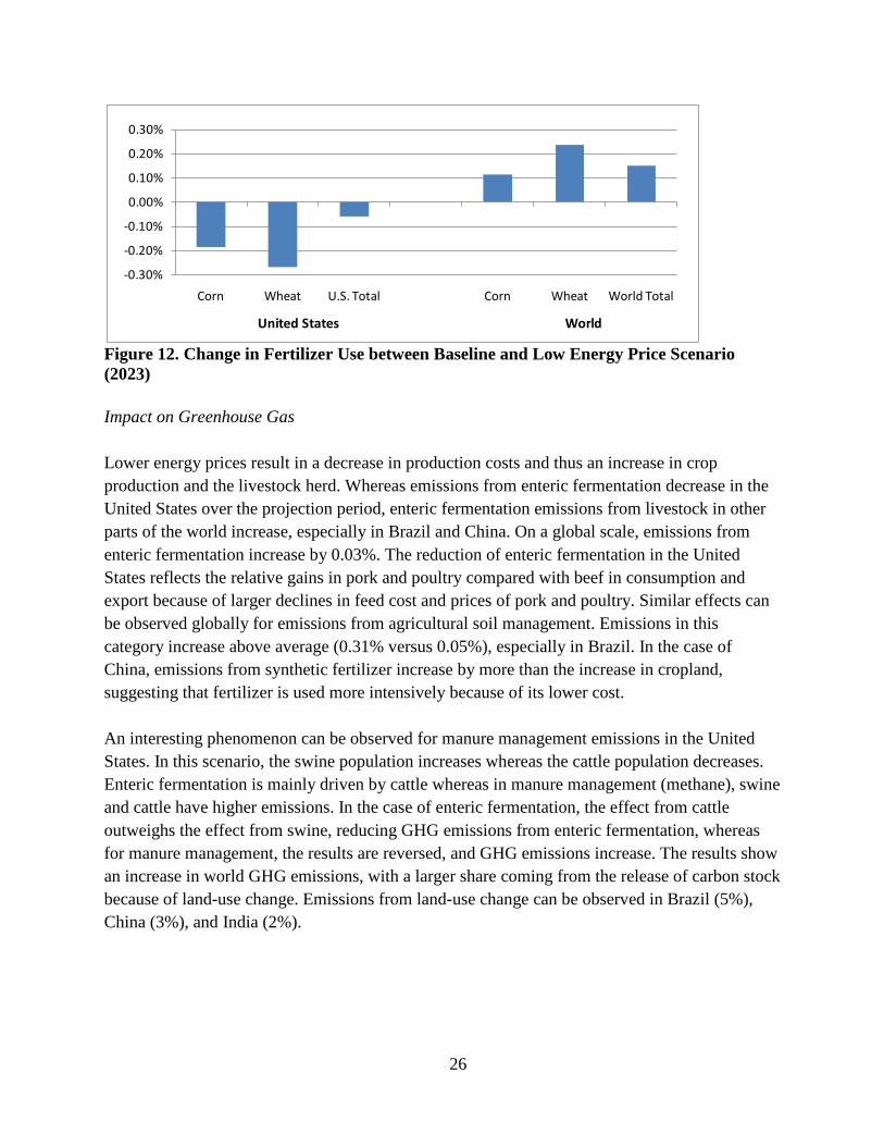
Because U.S. wheat and corn exports are a substantial share of their respective total utilization, the unfavorable export demand shock overwhelms the favorable supply shock such that wheat and corn area and production in the United States decline even with slightly higher yields (Figure 10). Figure 11 shows that U.S. net exports follow the same pattern. In contrast, increases in production of the three commodities are observed in the rest of the world where total area expansion occurs more readily than in the United States. Demand and supply rigidities in the U.S. ethanol retail and blender markets caused by policies induce a relatively large decline in wholesale and retail ethanol prices compared with the baseline. For the case of biodiesel, production in the United States expands even when the price of the fuel declines. This follows because the global expansion in soybean production results in lower soybean oil prices, the main feedstock used in the United States. Conversely, production declines in the rest of the world as the costs of major feedstocks utilized in the European Union and Southeast Asia decline by a lesser extent relative to soybean oil. Lower energy prices impact the livestock sector mostly through a reduction in feed costs. Therefore, while we see a decline in the price of all meats (see Table 4), the impacts are more pronounced in pork and poultry compared with beef, as beef production declines (see Figure 10). This is to be expected because pork and poultry production use feed more intensively, relative to beef production, and hence the costs of production fall by a higher amount. In summary, with the lower cost of production, we find that there is both extensification and intensification in the crops sector, expanding supply and lowering prices. As a result, the livestock and dairy sectors gain from the lower feed cost, thereby increasing production and lowering prices. Impact on Fertilizer Figure 12 shows that total fertilizer use moves in opposite directions between the United States and the world as a result of the low energy price scenario. Total fertilizer use in the United States decreases although N demand remains almost constant while P and K both decrease. The higher fertilizer application rate across all commodities due to reduction in the N, P, and K prices is not sufficient to offset the decrease in harvested areas of corn, wheat, sugarcane, and sugar beet. In contrast, total world fertilizer use increases as a result of a generalized increase in the total fertilizer use of all commodities. For all commodities, the higher fertilizer application rates per hectare (due to lower fertilizer prices) dominate those cases in which the world harvested area decreases or remains constant.

26

Figure 12. Change in Fertilizer Use between Baseline and Low Energy Price Scenario (2023) Impact on Greenhouse Gas Lower energy prices result in a decrease in production costs and thus an increase in crop production and the livestock herd. Whereas emissions from enteric fermentation decrease in the United States over the projection period, enteric fermentation emissions from livestock in other parts of the world increase, especially in Brazil and China. On a global scale, emissions from enteric fermentation increase by 0.03%. The reduction of enteric fermentation in the United States reflects the relative gains in pork and poultry compared with beef in consumption and export because of larger declines in feed cost and prices of pork and poultry. Similar effects can be observed globally for emissions from agricultural soil management. Emissions in this category increase above average (0.31% versus 0.05%), especially in Brazil. In the case of China, emissions from synthetic fertilizer increase by more than the increase in cropland, suggesting that fertilizer is used more intensively because of its lower cost. An interesting phenomenon can be observed for manure management emissions in the United States. In this scenario, the swine population increases whereas the cattle population decreases. Enteric fermentation is mainly driven by cattle whereas in manure management (methane), swine and cattle have higher emissions. In the case of enteric fermentation, the effect from cattle outweighs the effect from swine, reducing GHG emissions from enteric fermentation, whereas for manure management, the results are reversed, and GHG emissions increase. The results show an increase in world GHG emissions, with a larger share coming from the release of carbon stock because of land-use change. Emissions from land-use change can be observed in Brazil (5%), China (3%), and India (2%).

-0.30%

-0.20%

-0.10%

0.00%

0.10%

0.20%

0.30%

Corn Wheat U.S. Total Corn Wheat World Total

United States World

27

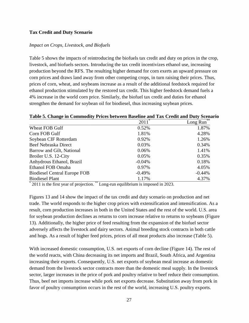
Tax Credit and Duty Scenario Impact on Crops, Livestock, and Biofuels Table 5 shows the impacts of reintroducing the biofuels tax credit and duty on prices in the crop, livestock, and biofuels sectors. Introducing the tax credit incentivizes ethanol use, increasing production beyond the RFS. The resulting higher demand for corn exerts an upward pressure on corn prices and draws land away from other competing crops, in turn raising their prices. Thus, prices of corn, wheat, and soybeans increase as a result of the additional feedstock required for ethanol production stimulated by the restored tax credit. This higher feedstock demand fuels a 4% increase in the world corn price. Similarly, the biofuel tax credit and duties for ethanol strengthen the demand for soybean oil for biodiesel, thus increasing soybean prices. Table 5. Change in Commodity Prices between Baseline and Tax Credit and Duty Scenario

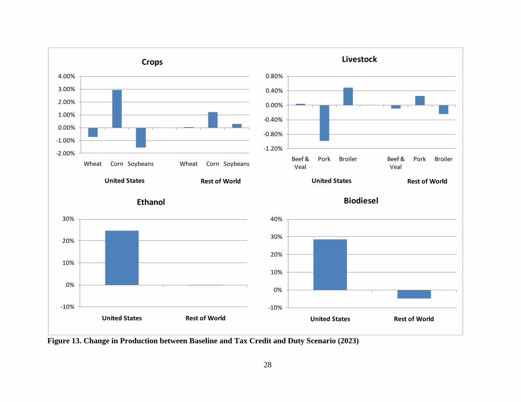
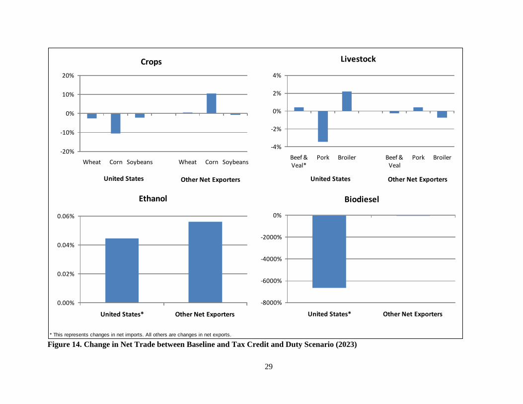
2011* Long Run** Wheat FOB Gulf 0.52% 1.87% Corn FOB Gulf 1.81% 4.28% Soybean CIF Rotterdam 0.92% 1.26% Beef Nebraska Direct 0.03% 0.34% Barrow and Gilt, National 0.06% 1.41% Broiler U.S. 12-City 0.05% 0.35% Anhydrous Ethanol, Brazil -0.04% 0.18% Ethanol FOB Omaha 0.97% 4.05% Biodiesel Central Europe FOB -0.49% -0.44% Biodiesel Plant 1.17% 4.37% * 2011 is the first year of projection. ** Long-run equilibrium is imposed in 2023. Figures 13 and 14 show the impact of the tax credit and duty scenario on production and net trade. The world responds to the higher crop prices with extensification and intensification. As a result, corn production increases in both in the United States and the rest of the world. U.S. area for soybean production declines as returns to corn increase relative to returns to soybeans (Figure 13). Additionally, the higher price of feed resulting from the expansion of the biofuel sector adversely affects the livestock and dairy sectors. Animal breeding stock contracts in both cattle and hogs. As a result of higher feed prices, prices of all meat products also increase (Table 5). With increased domestic consumption, U.S. net exports of corn decline (Figure 14). The rest of the world reacts, with China decreasing its net imports and Brazil, South Africa, and Argentina increasing their exports. Consequently, U.S. net exports of soybean meal increase as domestic demand from the livestock sector contracts more than the domestic meal supply. In the livestock sector, larger increases in the price of pork and poultry relative to beef reduce their consumption. Thus, beef net imports increase while pork net exports decrease. Substitution away from pork in favor of poultry consumption occurs in the rest of the world, increasing U.S. poultry exports.

28

Figure 13. Change in Production between Baseline and Tax Credit and Duty Scenario (2023)

-2.00%

-1.00%

0.00%

1.00%

2.00%

3.00%

4.00%


Crops


-1.20%

-0.80%

-0.40%

0.00%

0.40%

0.80%

Beef & Veal


Pork Broiler

Livestock


-10%

0%

10%

20%

30%


Ethanol

-10%

0%

10%

20%

30%

40%


Biodiesel

29

Figure 14. Change in Net Trade between Baseline and Tax Credit and Duty Scenario (2023)* This represents changes in net imports. All others are changes in net exports.

-20%

-10%

0%

10%

20%


Crops


-4%

-2%

0%

2%

4%

Beef & Veal*


Pork Broiler

Livestock


0.00%

0.02%

0.04%

0.06%


Ethanol

-8000%

-6000%

-4000%

-2000%

0%


Biodiesel

30

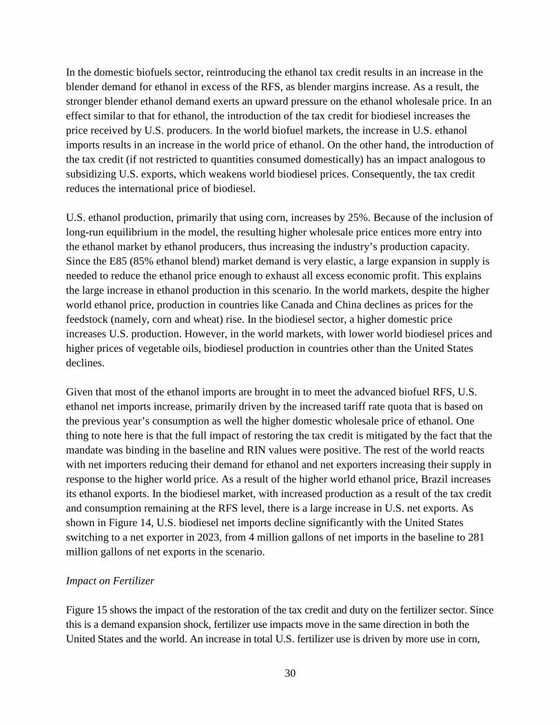
In the domestic biofuels sector, reintroducing the ethanol tax credit results in an increase in the blender demand for ethanol in excess of the RFS, as blender margins increase. As a result, the stronger blender ethanol demand exerts an upward pressure on the ethanol wholesale price. In an effect similar to that for ethanol, the introduction of the tax credit for biodiesel increases the price received by U.S. producers. In the world biofuel markets, the increase in U.S. ethanol imports results in an increase in the world price of ethanol. On the other hand, the introduction of the tax credit (if not restricted to quantities consumed domestically) has an impact analogous to subsidizing U.S. exports, which weakens world biodiesel prices. Consequently, the tax credit reduces the international price of biodiesel. U.S. ethanol production, primarily that using corn, increases by 25%. Because of the inclusion of long-run equilibrium in the model, the resulting higher wholesale price entices more entry into the ethanol market by ethanol producers, thus increasing the industry’s production capacity. Since the E85 (85% ethanol blend) market demand is very elastic, a large expansion in supply is needed to reduce the ethanol price enough to exhaust all excess economic profit. This explains the large increase in ethanol production in this scenario. In the world markets, despite the higher world ethanol price, production in countries like Canada and China declines as prices for the feedstock (namely, corn and wheat) rise. In the biodiesel sector, a higher domestic price increases U.S. production. However, in the world markets, with lower world biodiesel prices and higher prices of vegetable oils, biodiesel production in countries other than the United States declines. Given that most of the ethanol imports are brought in to meet the advanced biofuel RFS, U.S. ethanol net imports increase, primarily driven by the increased tariff rate quota that is based on the previous year’s consumption as well the higher domestic wholesale price of ethanol. One thing to note here is that the full impact of restoring the tax credit is mitigated by the fact that the mandate was binding in the baseline and RIN values were positive. The rest of the world reacts with net importers reducing their demand for ethanol and net exporters increasing their supply in response to the higher world price. As a result of the higher world ethanol price, Brazil increases its ethanol exports. In the biodiesel market, with increased production as a result of the tax credit and consumption remaining at the RFS level, there is a large increase in U.S. net exports. As shown in Figure 14, U.S. biodiesel net imports decline significantly with the United States switching to a net exporter in 2023, from 4 million gallons of net imports in the baseline to 281 million gallons of net exports in the scenario. Impact on Fertilizer Figure 15 shows the impact of the restoration of the tax credit and duty on the fertilizer sector. Since this is a demand expansion shock, fertilizer use impacts move in the same direction in both the United States and the world. An increase in total U.S. fertilizer use is driven by more use in corn,

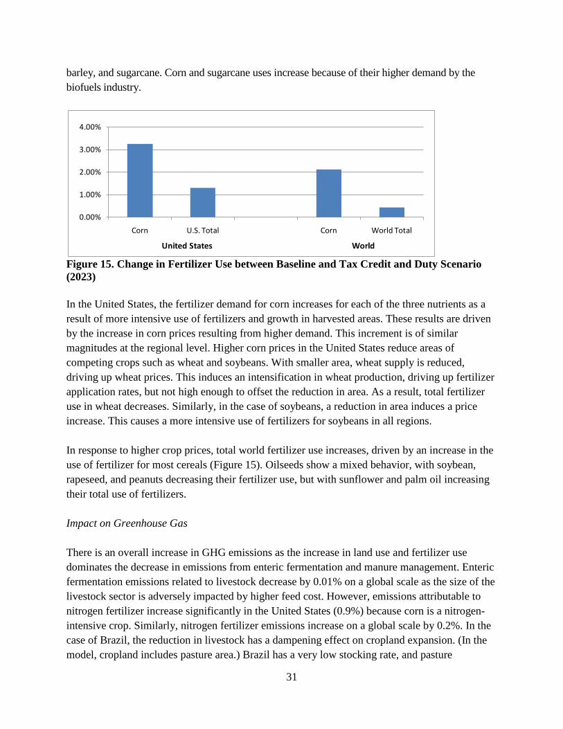
31

barley, and sugarcane. Corn and sugarcane uses increase because of their higher demand by the biofuels industry.

Figure 15. Change in Fertilizer Use between Baseline and Tax Credit and Duty Scenario (2023) In the United States, the fertilizer demand for corn increases for each of the three nutrients as a result of more intensive use of fertilizers and growth in harvested areas. These results are driven by the increase in corn prices resulting from higher demand. This increment is of similar magnitudes at the regional level. Higher corn prices in the United States reduce areas of competing crops such as wheat and soybeans. With smaller area, wheat supply is reduced, driving up wheat prices. This induces an intensification in wheat production, driving up fertilizer application rates, but not high enough to offset the reduction in area. As a result, total fertilizer use in wheat decreases. Similarly, in the case of soybeans, a reduction in area induces a price increase. This causes a more intensive use of fertilizers for soybeans in all regions. In response to higher crop prices, total world fertilizer use increases, driven by an increase in the use of fertilizer for most cereals (Figure 15). Oilseeds show a mixed behavior, with soybean, rapeseed, and peanuts decreasing their fertilizer use, but with sunflower and palm oil increasing their total use of fertilizers. Impact on Greenhouse Gas There is an overall increase in GHG emissions as the increase in land use and fertilizer use dominates the decrease in emissions from enteric fermentation and manure management. Enteric fermentation emissions related to livestock decrease by 0.01% on a global scale as the size of the livestock sector is adversely impacted by higher feed cost. However, emissions attributable to nitrogen fertilizer increase significantly in the United States (0.9%) because corn is a nitrogen-intensive crop. Similarly, nitrogen fertilizer emissions increase on a global scale by 0.2%. In the case of Brazil, the reduction in livestock has a dampening effect on cropland expansion. (In the model, cropland includes pasture area.) Brazil has a very low stocking rate, and pasture

0.00%

1.00%

2.00%

3.00%

4.00%

Corn U.S. Total Corn World Total

United States World

32

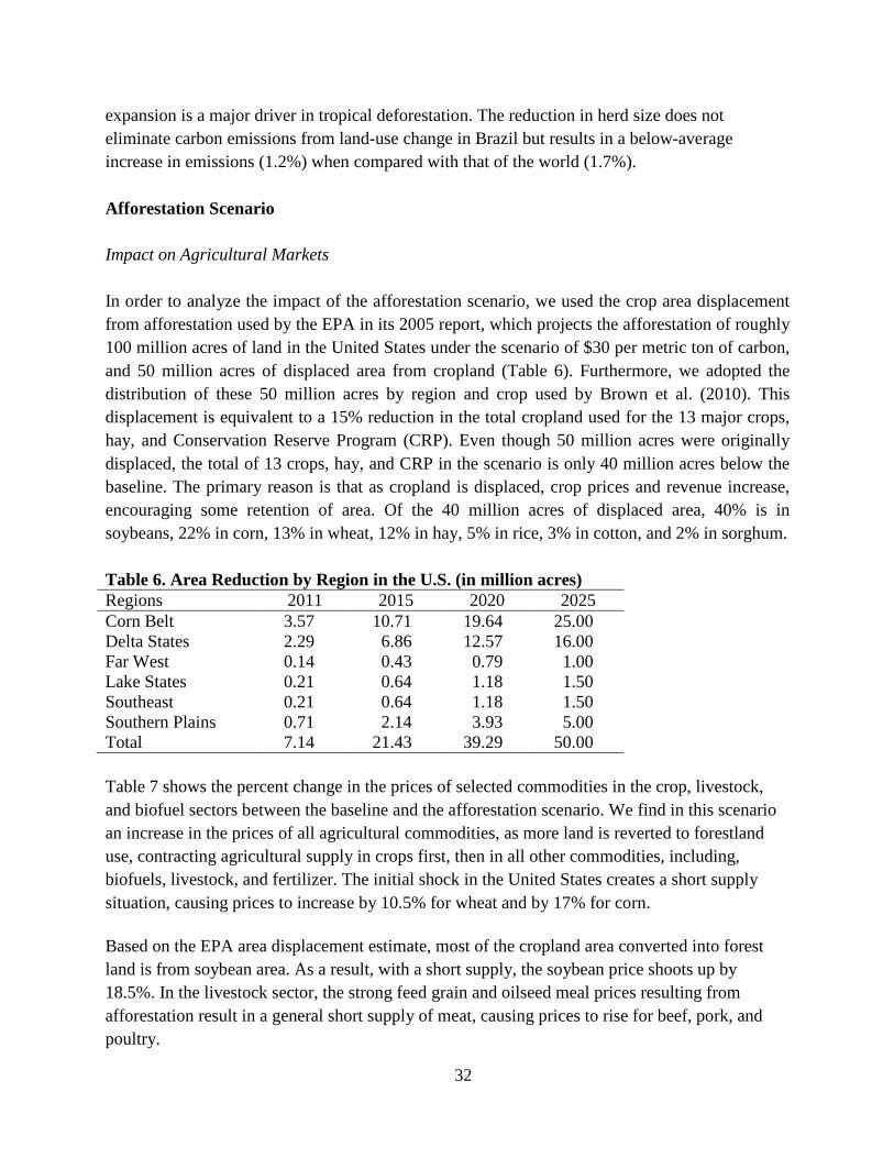
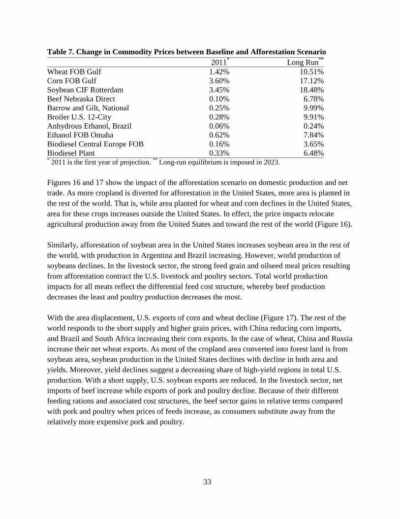
expansion is a major driver in tropical deforestation. The reduction in herd size does not eliminate carbon emissions from land-use change in Brazil but results in a below-average increase in emissions (1.2%) when compared with that of the world (1.7%). Afforestation Scenario Impact on Agricultural Markets In order to analyze the impact of the afforestation scenario, we used the crop area displacement from afforestation used by the EPA in its 2005 report, which projects the afforestation of roughly 100 million acres of land in the United States under the scenario of $30 per metric ton of carbon, and 50 million acres of displaced area from cropland (Table 6). Furthermore, we adopted the distribution of these 50 million acres by region and crop used by Brown et al. (2010). This displacement is equivalent to a 15% reduction in the total cropland used for the 13 major crops, hay, and Conservation Reserve Program (CRP). Even though 50 million acres were originally displaced, the total of 13 crops, hay, and CRP in the scenario is only 40 million acres below the baseline. The primary reason is that as cropland is displaced, crop prices and revenue increase, encouraging some retention of area. Of the 40 million acres of displaced area, 40% is in soybeans, 22% in corn, 13% in wheat, 12% in hay, 5% in rice, 3% in cotton, and 2% in sorghum. Table 6. Area Reduction by Region in the U.S. (in million acres) Regions 2011 2015 2020 2025 Corn Belt 3.57 10.71 19.64 25.00 Delta States 2.29 6.86 12.57 16.00 Far West 0.14 0.43 0.79 1.00 Lake States 0.21 0.64 1.18 1.50 Southeast 0.21 0.64 1.18 1.50 Southern Plains 0.71 2.14 3.93 5.00 Total 7.14 21.43 39.29 50.00 Table 7 shows the percent change in the prices of selected commodities in the crop, livestock, and biofuel sectors between the baseline and the afforestation scenario. We find in this scenario an increase in the prices of all agricultural commodities, as more land is reverted to forestland use, contracting agricultural supply in crops first, then in all other commodities, including, biofuels, livestock, and fertilizer. The initial shock in the United States creates a short supply situation, causing prices to increase by 10.5% for wheat and by 17% for corn. Based on the EPA area displacement estimate, most of the cropland area converted into forest land is from soybean area. As a result, with a short supply, the soybean price shoots up by 18.5%. In the livestock sector, the strong feed grain and oilseed meal prices resulting from afforestation result in a general short supply of meat, causing prices to rise for beef, pork, and poultry.

33

Table 7. Change in Commodity Prices between Baseline and Afforestation Scenario 2011* Long Run**

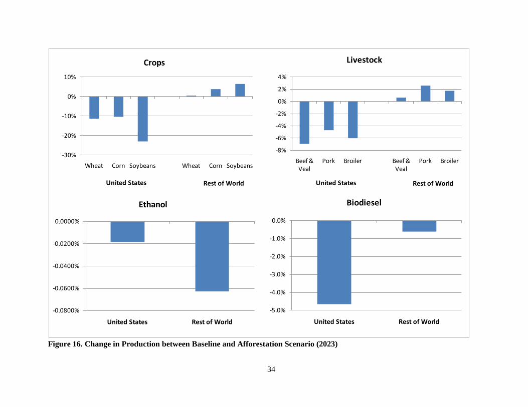
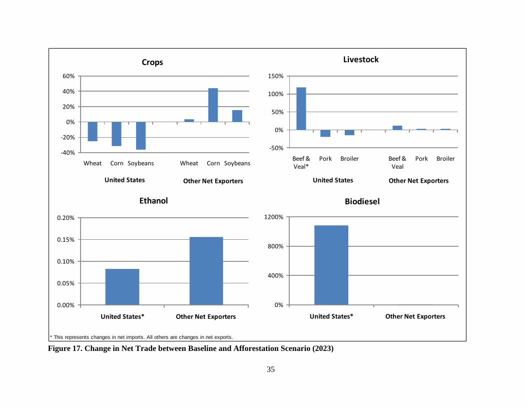
Wheat FOB Gulf 1.42% 10.51% Corn FOB Gulf 3.60% 17.12% Soybean CIF Rotterdam 3.45% 18.48% Beef Nebraska Direct 0.10% 6.78% Barrow and Gilt, National 0.25% 9.99% Broiler U.S. 12-City 0.28% 9.91% Anhydrous Ethanol, Brazil 0.06% 0.24% Ethanol FOB Omaha 0.62% 7.84% Biodiesel Central Europe FOB 0.16% 3.65% Biodiesel Plant 0.33% 6.48% * 2011 is the first year of projection. ** Long-run equilibrium is imposed in 2023. Figures 16 and 17 show the impact of the afforestation scenario on domestic production and net trade. As more cropland is diverted for afforestation in the United States, more area is planted in the rest of the world. That is, while area planted for wheat and corn declines in the United States, area for these crops increases outside the United States. In effect, the price impacts relocate agricultural production away from the United States and toward the rest of the world (Figure 16). Similarly, afforestation of soybean area in the United States increases soybean area in the rest of the world, with production in Argentina and Brazil increasing. However, world production of soybeans declines. In the livestock sector, the strong feed grain and oilseed meal prices resulting from afforestation contract the U.S. livestock and poultry sectors. Total world production impacts for all meats reflect the differential feed cost structure, whereby beef production decreases the least and poultry production decreases the most. With the area displacement, U.S. exports of corn and wheat decline (Figure 17). The rest of the world responds to the short supply and higher grain prices, with China reducing corn imports, and Brazil and South Africa increasing their corn exports. In the case of wheat, China and Russia increase their net wheat exports. As most of the cropland area converted into forest land is from soybean area, soybean production in the United States declines with decline in both area and yields. Moreover, yield declines suggest a decreasing share of high-yield regions in total U.S. production. With a short supply, U.S. soybean exports are reduced. In the livestock sector, net imports of beef increase while exports of pork and poultry decline. Because of their different feeding rations and associated cost structures, the beef sector gains in relative terms compared with pork and poultry when prices of feeds increase, as consumers substitute away from the relatively more expensive pork and poultry.

34

Figure 16. Change in Production between Baseline and Afforestation Scenario (2023)

-30%

-20%

-10%

0%

10%


Crops


-8%

-6%

-4%

-2%

0%

2%

4%

Beef & Veal


Pork Broiler

Livestock


-0.0800%

-0.0600%

-0.0400%

-0.0200%

0.0000%


Ethanol

-5.0%

-4.0%

-3.0%

-2.0%

-1.0%

0.0%


Biodiesel

35

Figure 17. Change in Net Trade between Baseline and Afforestation Scenario (2023)* This represents changes in net imports. All others are changes in net exports.

-40%

-20%

0%

20%

40%

60%


Crops


-50%

0%

50%

100%

150%

Beef & Veal*


Pork Broiler

Livestock


0.00%

0.05%

0.10%

0.15%

0.20%


Ethanol

0%

400%

800%

1200%


Biodiesel

36

Impact on Fertilizer Total fertilizer use in the United States decreases by 14% because of the reduction in crop area from shifts to forest land. The lower supply increases crop prices, which contributes to the intensification of production in all U.S. regions. Total U.S. demand of N, P, and K decreases because the area reduction dominates. Higher corn prices in the United States induce the more intensive use of fertilizers in all regions, and, as a result, fertilizer application rates in corn increase in each region. However, the fertilizer application rates for the aggregate United States are reduced. The reason is that the corn area reallocation is such that those areas less intensive in the use of fertilizers (such as the Northern Plains, Northeast, and Delta States) increase, and areas more intensive in the use of fertilizer in corn (such as the Corn Belt and Southern Plains) decrease. Therefore, because of both the reduction in areas and the lower application rates, fertilizer demand for corn in the United States decreases. A similar effect occurs in wheat and soybeans, with a slight exception in soybeans, where expansion occurs in regions (such as the Northern Plains and Delta States) that are more intensive in the use of N but less intensive in the use of P and K. In several other countries, total fertilizer use increases because of price-induced intensification in all commodities. However, world total fertilizer use decreases by 1% as a result of both the reduction in crop areas in the United States and the shift in production to countries with lower-than-average fertilizer application rates. Total fertilizer use at the world level decreases by 2.30% in corn, by 0.45% in wheat, and by 6.13% in soybeans. Impact on Greenhouse Gas The afforestation scenario represents a major shift in U.S. agricultural production, and we see that the unintended consequence of this policy is an increase in carbon emissions from land-use change on a global scale. Emissions from enteric fermentation decrease for all major countries as most livestock and dairy sectors contract under a high feed regime with afforestation, with the sharpest decrease occurring in the United States (1.037%). Emissions from nitrogen application are reduced by 0.39% on a global scale. The main driver for this result is the U.S. cropland reduction, although fertilizer consumption in most other countries increases. For example, total fertilizer emissions increase by 0.856% in Brazil, by 0.695% in China, and by 0.268% in the European Union. The most interesting aspect of the scenario is the increase in carbon emissions related to land-use change in the rest of the world. High-quality U.S. cropland is replaced with lower quality cropland (quality in terms of yield), and hence, more area is needed to compensate for the reduction in production. We see cropland increase in almost all countries, including in Brazil (0.212%) and China (0.635%). Because many of these countries have exhausted their idle

37

cropland, any increase in cropland is likely to be supplied by converting land covered by native vegetation, leading to a 6.65% increase in global emissions from land-use change compared with the baseline.

5. Summary and Conclusion This analysis evaluates the impact of four alternative scenarios on U.S. and world agricultural markets, as well as on world fertilizer use and world agricultural greenhouse gas emissions. A key assumption in the baseline is that ethanol support policies disappear in 2012. The baseline also assumes that existing biofuel mandates remain in place and are binding. Two of the scenarios are adverse supply shocks, the first being a 10% increase in the price of nitrogen fertilizer in the United States, and the second, a reversion of cropland into forestland. The third scenario examines how lower energy prices would impact world agriculture. The fourth scenario reintroduces biofuel tax credits and duties. Given that the baseline excludes these policies, the fourth scenario is an attempt to understand the impact of these policies under the market conditions that prevailed in early 2011. A key to understanding the results of this fourth scenario is that in the absence of tax credits and duties, the mandate drives biofuel use. Therefore, when the tax credits and duties are reintroduced, the impacts are relatively small. At the end of the baseline projection period, the United States accounts for 18% of the world’s idle cropland, Brazil 43%, Russia 10%, and Mexico 9%. Many of the remaining countries have almost exhausted their idle cropland, including Argentina with only 0.09 million hectares, Australia with 0.46, Canada with 1.30, China with 0.97, India with 0.02, and South Africa with 0.04. This situation is important because, in effect, any shock penalizing the United States in the sense of reducing U.S. cropland and thereby reducing U.S. exports may result in unintended consequences elsewhere, with countries that are short of cropland responding to this new market incentive and expanding domestic production by converting native vegetation, thus releasing rich carbon stock. In the livestock sector, the most interesting lesson from the scenarios is that they have a differential impact by meat type because of differences in cost structures across sectors. That is, feed cost accounts for only 28% of the total cost in a cow-calf operation while it accounts for 74% of a farrow-to-finish operation. Any shock in the United States that raises crop prices will automatically result in relatively higher price changes in pork and poultry compared with beef, which sustains domestic beef consumption through substitution and weakens any reduction of the beef sector from the higher crop prices. Also, pasture-based production systems in other countries may not be too adversely affected by higher grain prices, allowing expansion in world beef production and a dramatic increase in world GHG emissions.

38

The impact of a policy that raises nitrogen fertilizer prices on GHG emissions is muted when the entire agricultural sector in the world market is allowed to adjust. For example, although fertilizer-intensive crops (such as corn) are penalized with higher nitrogen fertilizer prices resulting in lower fertilizer use, more fertilizer is used in the same crops in the rest of the world. Moreover, market rigidities caused by policies dull the impact of higher nitrogen fertilizer prices. This is particularly true in biofuels, which have a binding RFS in both ethanol and biodiesel production in the baseline. Higher corn feedstock prices reduce domestic production of ethanol. But because the RFS is binding, any reduction in domestic corn ethanol is simply replaced by an increase in the imports of sugarcane ethanol from Brazil, thereby raising the world ethanol price, sugarcane area, and sugarcane fertilizer use. The low energy price scenario increases fertilizer use, area, and GHG emissions as agricultural production of both crop and animal enterprises expand. The exception in this case is the United States, where despite the more intensive use of fertilizer per hectare in all crops, total fertilizer use in corn and wheat decrease because of the reduction in harvested area, induced by the lower demand. The reintroduction of tax credits and duties in the U.S. biofuel sector increases area, production, fertilizer, and GHG emissions as this policy shock incentivizes expansion of biofuel demand. However, the impact is muted because most of the tax credit is used to offset RIN values, which represent the binding mandate. In the afforestation scenario, crop production shifts from high-yielding land in the United States to low-yielding land in the rest of the world. Moreover, there is an increased likelihood that land with native vegetation will be converted into cropland. The net impact is an unintended increase in world GHG emissions. In general, the results show that the entire international commodity market system is remarkably robust with respect to policy changes in one country or in one sector. The policy implication is that domestic policy changes implemented by a large agricultural producer like the United States can have fairly significant impacts on the aggregate world commodity markets. A second point that emerges from the results is that the law of unintended consequences is at work in world agriculture. For example, a U.S. nitrogen tax that might presumably be motivated for environmental benefit results in an increase in world greenhouse gas emissions.

39

References

Brown, T., A. Elobeid, J. Dumortier, and D.J. Hayes. 2010. “Market Impact of Domestic Offset Programs.” CARD Working Paper 10-WP 502, Center for Agricultural and Rural Development, Iowa State University.

Du, X., and D.J. Hayes. 2011. “The Impact of Ethanol Production on US and Regional Gasoline

Markets: An Update to May 2009.” CARD Working Paper 11-WP 523, Center for Agricultural and Rural Development, Iowa State University.

Dumortier, J., D.J. Hayes, M. Carriquiry, F. Dong, X. Du, A. Elobeid, J.F. Fabiosa, and K.

Mulik. 2010. “Modeling the Effects of Pasture Expansion on Emissions from Land-Use Change.”CARD Working Paper 10-WP 504, Center for Agricultural and Rural Development, Iowa State University.

Environmental Protection Agency (EPA). 2005. Greenhouse Gas Mitigation Potential in U.S.

Forestry and Agriculture. EPA 430-R-05-006. U.S. EPA, Office of Atmospheric Programs. Washington, DC.

Food and Agricultural Policy Research Institute, University of Missouri (FAPRI-MU). 2010.

“U.S. Biofuels, Corn Processing, Distillers Grains, Fats, Switchgrass, and Corn Stover Model Documentation .” FAPRI-MU Report #09-10, FAPRI, University of Missouri-Columbia.

Hayes, D., B. Babcock, J. Fabiosa, S. Tokgoz, A. Elobeid, T.-H. Yu, et al. 2009. “Biofuels:

Potential Production Capacity, Effects on Grain and Livestock Sectors, and Implications for Food Prices and Consumers.” Journal of Agricultural and Applied Economics 41(2): 1–27.

Muller, A., J. Schmidhuber, J. Hoogeveen, and P. Steduto. 2007. “Some Insight in the Effect of

Growing Bio-Energy Demand on Global Food Security and Natural Resources.” Paper presented at the International Conference “Linkages between Energy and Water Management for Agriculture in Developing Countries,” Hyderabad, India, 28-31 January.

Rosas, F. 2011. “The Worlds Fertilizer Model—World NPK Model.” CARD Working Paper 11-WP 520, Center for Agricultural and Rural Development, Iowa State University.

Tokgoz, S., A. Elobeid, J.F. Fabiosa, D.J. Hayes, B.A. Babcock, T.-H. Yu, F. Dong, C.E. Hart,

and J.C. Beghin. 2007. “Emerging Biofuels: Outlook of Effects on U.S. Grain, Oilseed, and Livestock Markets.” CARD Staff Report 07-SR 101, Center for Agricultural and Rural Development, Iowa State University.

U.S. Department of Agriculture (USDA). 2009. “The Impacts of the American Clean Energy and

Security Act of 2009 on U.S. Agriculture”, Office of the Chief Economist, ERS-USDA, December 18, 2009. http://www.usda.gov/oce/newsroom/archives/releases/2009files/ImpactsofHR%202454.pdf

http://www.usda.gov/oce/newsroom/archives/releases/2009files/ImpactsofHR%202454.pdf

40

U.S. Department of Agriculture (USDA). 2010. “EU-27. Biofuels Annual.” http://gain.fas.usda.gov/Recent%20GAIN%20Publications/ General%20Report_The%20Hague_Netherlands-Germany%20EU-27_6-15-2009.pdf

U.S. Energy Information Administration (EIA). 2011. World Crude Oil Prices.

http://www.eia.doe.gov/dnav/pet/PET_PRI_WCO_K_W.htm (accessed May 19, 2011).

http://gain.fas.usda.gov/Recent%20GAIN%20Publications/General%20Report_The%20Hague_Netherlands-Germany%20EU-27_6-15-2009.pdf

http://gain.fas.usda.gov/Recent%20GAIN%20Publications/General%20Report_The%20Hague_Netherlands-Germany%20EU-27_6-15-2009.pdf

http://www.eia.doe.gov/dnav/pet/PET_PRI_WCO_K_W.htm

41

Appendix

The appendix tables with detailed scenario results by country and commodity are available at http://www.card.iastate.edu/publications/synopsis.aspx?id=1161.

http://www.card.iastate.edu/publications/synopsis.aspx?id=1161

Documents

Greenhouse Gas and Nitrogen Fertilizer Scenarios for U.S