Green Technology Adoption: An Empirical Study of the

Southern California Garment Cleaning Industry ∗

Bryan Bollinger, NYU

July 10, 2014

Abstract

Firms may be slow to adopt green technologies without sufficient private incentives to do

so, or because of long equipment replacement cycles or lack of information. In California, reg-

ulators implemented multiple types of policies to overcome these obstacles in order to reduce

the use of the polluting technology used in traditional dry cleaning. I evaluate the effective-

ness of these different policy tools using a dynamic, durable good replacement model with

entry and exit for garment cleaning firms in southern California. I control for and exploit the

changing policies to estimate the effects of financial incentives, strict command-and-control

regulations, and green technology demonstrations on cleaners’ equipment purchases. Further-

more, because the command-and-control regulations only regulate future equipment use and

purchases, I am also able to estimate cleaners’ discount rate. In the counterfactual analyses, I

find that multi-pronged approach increases welfare more than any of the single policies taken

in isolation. Furthermore, the welfare gains from reducing air pollution are an order of magni-

tude greater than the costs associated with any of the policies, and since I find that cumulative

green adoption would remain below than 30% without strict command-and-control regula-

tions, the strict regulations imposed are second best in terms of overall welfare.

∗I would like to thank Harikesh Nair, Sridhar Narayanan, and Peter Reiss for their helpful comments as well asthe two anonymous referees for their insightful feedback. I would especially like to thank Wesley Hartmann for hisinvaluable support and guidance throughout. All remaining mistakes are my own.

1

1 Introduction

The adoption of new, cleaner technologies is essential in reducing air and water pollution, which is

an increasingly important and visible issue, with serious health and environmental consequences.

Even if the technologies have already been developed, the empirical technology diffusion litera-

ture has demonstrated that the diffusion of new technologies can be slow Bass (1969), Mahajan

et al. (1990), Hannan & McDowell (1984), Mulligan (2003), Baker (2001), Engers et al. (2009). There

exist a variety of potential explanations for slow adoption: i) firms do not realize the full societal

benefits of using the green technology and the green technology is not superior in terms of the

firms’ private incentives; ii) firms may have long equipment replacement cycles which slow the

migration to a socially and privately better technology; or iii) firms may not have sufficient in-

formation to evaluate whether or not a switch to a green technology is in their private interests.1

Government intervention is often used to expedite the adoption of the cleaner technologies, in

order to reduce the difference in the private and social values of adoption.

When dynamic effects must be considered, as in the case of durable goods, it is becoming more

common in the marketing and economics literatures to structurally model an agent’s decision to

adopt a new technology (Gowrisankaran & Stavins 2004, Tucker 2008, Gordon 2009). A structural

analysis of firms’ adoption decisions allows me to estimate policy-invariant profit function param-

eters which can be used to assess the different tools used by policymakers, or firms, to expedite

the adoption of the different technologies. In this paper, I study the garment cleaning industry

which i) involves the purchase of durable goods and faces just such a mix of policies to drive

adoption; ii) has readily available public data; and iii) has experienced variation in the types of

policies used over time that have altered both current variables and the expectations of the future,

which drive the identification of the parameters in dynamic models. The exogenously changing

environmental policies in southern California helps identify both the distribution of heterogeneity

in firms’ profit parameters and the discount factor, which I then use to evaluate the different types

of policies used, including financial incentives in the form of both grants and fees, the provision of

1The theory literature on technology adoption has demonstrated that uncertainty in new technologies may createbarriers to adoption, which are even larger in the case of durable goods (Jensen 1982, Farzin et al. 1998, Doraszelski2001).

1

training and information through the use of demonstration sites, and strict command-and-control

regulations.

I construct and estimate a single agent, dynamic durable good adoption model adapted from

Rust (1987) that explicitly solves for firms’ solutions to their dynamic optimization problems, as is

common in the literature (Nair 2007, Hartmann & Nair 2010, Smith 2010). I estimate the structural

primitives of the model using importance sampling (Ackerberg 2009) as done in Hartmann (2006),

Bajari et al. (2010), and Goettler & Clay (2010) in order to include rich heterogeneity which I would

expect due to the environmental nature of the application. Potential reasons for heterogeneity in

profits when using different types of equipment include differences in marginal costs or in the

prices firms are able to charge consumers for cleaning since the demand for cleaning equipment

reflects the demand for garment cleaning. I find that California’s current combination of finan-

cial incentives, in the form of both taxes and grants, and strict command-and-control regulations

lead to an increase in overall welfare; furthermore, the combination of the three policy tools to-

gether have greater long-run welfare gains than any one in isolation. The provision of information

and training through the wet cleaning demonstration sites further increases welfare and increases

adoption of the wet cleaning technology.

The rest of the paper is organized as follows: In Section 2, I discuss some of the relevant litera-

ture and provide background regarding the garment cleaning industry and the policies designed

to increase adoption of the cleaner technologies, and in Section 3 I describe the data. My model

and estimation strategy are outlined in Section 4 and the results are presented in Section 5. Sec-

tion 6 provides a discussion of the results and I use the structural parameter estimates to perform

counterfactual market simulations which are presented in Section 7. Section 8 concludes.

2

2 Background

2.1 Conceptual Background

Recently, there has been an increased focus on the adoption of green technologies in the field of

marketing (Narayanan & Nair 2012, Bollinger & Gillingham 2012, Shriver 2012). The main goal

of this paper is to model green technology adoption decisions by cleaners as a direct function of

different policy tools that can be used to alter the adoption rates. This allows me to perform coun-

terfactual analyses to assess the welfare implications of the different types of polices. Although

this paper concerns technology adoption decisions by firms, the data used is in many ways more

similar to that used in the literature on entry and exit games. While I have data on the type of

technology adopted, I do not have information on prices and quantities. However, the rich set

of policies used in California to alter firms’ adoption decisions more than offsets the limitations

that result from the lack of price/quantity data, since I directly measure the impact of policies

that were actually used. The structure of the model allows me to then separate the effects of each

policy tool in isolation.

In addition to green technology adoption, one would expect the policies to affect entry and exit

decisions. Therefore, to assess the entire impact of each policy tool, I need to allow for entry and

exit. Pakes et al. (2007) develop an estimation strategy that can be used in modeling dynamic en-

try and exit in the presence of firm heterogeneity. While this has been possible using frameworks

such as the Ericson & Pakes (1995) framework, computational limitations have often led to the use

of two-stage models instead (Bresnahan & Reiss 1991, Berry 1992, Mazzeo 2002, Seim 2006). Un-

fortunately, the Pakes et al. (2007) methodology is not suited for my purposes since the estimation

method, like two-stage methods such as Hotz & Miller (1993) and Bajari et al. (2007), depends on

the ability to estimate action probabilities in a first stage. However, since the policies used in this

application affect payoffs in future states which do not arise in the data, it is not possible to get

such estimates without extrapolating beyond the support of the data.

I instead use an importance sampling approach (Ackerberg 2009) to directly calculate value

functions which allows me to i) include rich, continuous heterogeneity on all of the firms’ profit

3

parameters; ii) estimate the structural parameters of the model which determine the state transi-

tion probabilities; iii) estimate the discount rate; iv) perform counterfactual analyses as the market

transitions (in some cases) to situations where the green technologies dominate. This is the only

application of importance sampling of which I am aware that includes entry and exit in a dynamic

setting with heterogeneity, controlling for the endogeneity of the initial market conditions. This is

important since to predict entry and exit under counterfactual scenarios, it is essential to uncover

the distribution of parameters for all potential cleaners, not just the realized distribution for those

who have selected to enter the market.

2.2 Industry Background

Laundry services and garment cleaning is a $22.6 billion dollar per year industry, according to the

2007 U.S. Census Bureau’s Annual Services Survey (Hambric 2008). The standard technology used

in garment cleaning requires the use of perchloroethylene (perc) as the solvent, a toxic, cancer-

causing air and ground contaminant used by approximately 28,000 U.S. dry cleaners nationwide

according to the Environmental Protection Agency (EPA). The issue is of such importance that

the State Coalition for Remediation of Drycleaners was established in 1998, with support from

the EPA, in order to aid in the development of remediation programs to clean up contamination

caused by the use of perc.2 A document was released by the EPA in 1992 summarizing the hazards

associated with exposure to perc, and since then the use of the chemical has come under more and

more scrutiny. Currently, the EPA is considering whether to compel dry cleaners to phase out

perc nationwide.3 The California Dry Cleaning Industry Technical Assessment Report was pub-

lished in 2006 as part of the 1993 Airborne Toxic Control Measure for Emissions of Perchloroethy-

lene from Dry Cleaning Operations and provides a detailed description of the California garment

cleaning industry (Fong et al. 2006). The California Air Resources Board (CAARB) 2003 facility

surveys estimated that there were around 5040 cleaners, 4,670 of which used perc.

Although the majority of cleaners use perc equipment, alternative cleaning technologies are

2Thirteen states are members of the coalition.3Washington Post, Wednesday, April 8, 2009, page A03. http://www.washingtonpost.com/wp-

dyn/content/article/2009/04/07/AR2009040703748.html

4

available. Each type of equipment is intended for use with a specific liquid solvent. All garment

cleaning processes involves the submersion of the garment in the solvent (including traditional

”dry” cleaning using perc) and the characteristics of the solvent, as well as how much escapes

during the process, determine the cleanliness of the technology. The four main technologies that

compete with perc cleaning are hydrocarbon (or fluorocarbon), GreenEarth, carbon dioxide, and

wet cleaning. Anecdotally, cleaner owners consider hydrocarbon cleaning to be the most similar to

perc. The cleanest technologies are carbon dioxide and wet cleaning since both use safe, naturally

occurring compounds, liquid carbon dioxide and water, respectively. The estimated costs for these

different types of equipment can be found in Table 2, along with average annual operating costs,

excluding labor.4 Carbon dioxide cleaning equipment is by far the most expensive. Wet cleaning

equipment is not very expensive, but the process is more complex – it requires a higher level of

control throughout the cleaning process and tensioning equipment is needed to restore clothes to

their original shape after wet cleaning. More training is required for employees when using wet

cleaning equipment in order to ensure the same level of efficacy.

The road to perc regulation began in 1991 when the CAARB determined that perc is a toxic air

contaminant which falls under California’s Toxic Air Contaminant Identification and Control Pro-

gram. In 1993, the CAARB adopted the Airborne Toxic Control Measure (ATCM) for Emissions

of Perc from Dry Cleaning Operations (Dry Cleaning ATCM) and the Environmental Training

Program for perc dry cleaning operations, setting new requirements for cleaners in an effort to re-

duce air contamination. In southern California, the South Coast Air Quality Management District

(SCAQMD)5 decided to eliminate the use of perc machines by the end of 2020 and disallow the

use of perc equipment over 15 years of age, recognizing the durable nature of the equipment in its

phase-out plan.6 At this time, the SCAQMD also instituted a grant program for cleaners switching

4More detail can be found in the CAARB California Dry Cleaning Industry Technical Assessment Report. Opera-tional costs follow the same trends as the machinery costs: Carbon dioxide cleaning has high capital and operationalcosts but wet cleaning actually has lower costs than traditional perc cleaning. However, this does not account for the ex-tra training required to use the greener technologies or the fact that wet cleaning is more labor intensive than traditionaldry cleaning.

5The SCAQMD is the air pollution control agency for all of Orange County and the urban portions of Los Angeles,Riverside and San Bernardino counties. It has well over half of the cleaners in the state.

6SCAQMD Rule 1421 was first passed on December 9, 1994, but the final version was updated December 6, 2002.It states that ”On or after January 1, 2003, an owner or operator of a new facility may not operate a perchloroethylenedry cleaning system. On or after December 6, 2002, an owner or operator of an existing facility shall be allowed tooperate its perchloroethylene dry cleaning system(s) until the end of its useful life and, upon replacement, shall beallowed to operate no more than one perchloroethylene dry cleaning system per facility until December 31, 2020.” The

5

to green technologies.

In August 2004, the CAARB added its own measures to reduce the use of perc, including its

own grants, the use of an increasing fee on the perc solvent, and the institution of a demonstration

program to provide dry cleaners with the opportunity to learn about green cleaning technology,

primarily wet cleaning, at various locations across California.7 The changing regulations and in-

centives are summarized in Table 1. The biggest shift in the regulations after 2003 was on January

25, 2007, when California legislators amended the Dry Cleaning ATCM to prohibit the sale or

lease of new perc dry cleaning machines, beginning on January 1, 2008. It is notable that while the

previously announced phase-out accounted for the restrictions placed upon cleaners due to the

expensive and durable nature of cleaning equipment, this new regulation did not since cleaners

had so little time to respond and no way of anticipating this shift in policy.

According to the president of the California Cleaners Association (CCA), the cleaners have

been working with the California Air Quality Management Districts across the state to try to limit

the financial costs of the phase-out but the many changes in the regulations were unanticipated

by the cleaners, who had limited ability to alter the legislation.8 The cleaners are being forced

to transition away from perc, and the CCA is now concerned that new legislation might force

cleaners away from the use of hydrocarbon cleaning as well, which is anecdotally considered by

many cleaners to be the most cost-effective technology after perc. According to the CCA, cleaners

are already being forced out of business by the new regulations and more restrictions will make

the problem considerably worse.

“useful life” of the equipment is something that came under rigorous debate between the SCAQMD and the CaliforniaCleaners Association(CCA), the SCAQMD wishing to set the useful life at ten years, the CCA at 20. A 15 year usefullife was the compromise.

7According to the CAARB website, ”Demonstration sites ultimately will, in time, create the regional and statewideinfrastructure necessary for the long-term diffusion of these technologies.”

8Even the compromise of 15 years as the regulated useful life of perc cleaning equipment is now potentially goingto be altered by the San Francisco Bay Area AQMD which is considering legislation to change the legal useful life ofperc equipment to 10 years.

6

3 Data

3.1 Data Description

The unique data set used in this paper is assembled from a variety of sources. The first source

is equipment permitting data from the SCAQMD; the data include each facility’s name, address

and phone number, as well as the type of equipment (perc or hydrocarbon), whether a permit

was granted (usually the case), the type of permit i.e. whether the permit is for a new piece of

equipment (new to the firm), and the date the permit was issued.9 The data on cleaners using hy-

drocarbon, wet, carbon dioxide or GreenEarth cleaning come from a variety of sources, including

lists of grant recipients from the SCAQMD and CAARB.10 In addition, a list of green cleaners from

the Urban & Environmental Policy Institute (UEPI) were also included.11 I also use SCAQMD per-

mit diary files to identify if a permit was inactivated in order to switch to a different technology.12

In addition to identifying cleaner actions in every year, these data allow me to construct the age

of cleaners’ equipment.13

The last piece of data concerns the demonstration sites. Under the CAARB demonstration

program, there were 52 demonstrations of either wet cleaning or carbon dioxide cleaning by the

end of 2009 at 28 different sites in California.14 In addition to the data on the location and timing

9A total of 15,204 permit applications by 9,381 cleaners were filed with the SCAQMD between 1956 and 2009, result-ing in 13,991 permits. In this analysis I treat cleaners after an ownership change as the same firm. Most of the cleanersthat appear in the SCAQMD data have perc equipment but some of the cleaners have equipment that use hydrocarbonor other petroleum solvents.

10There were 602 SCAQMD grants and 104 CAARB grants by the end of 2009.11The UEPI is a community oriented research and advocacy organization based at Occidental College in Los Angeles,

CA. Their website allows consumers to search for green cleaners (which they define to be wet or carbon dioxide clean-ers) that are within a given radius of a user-provided address. Their database included 166 wet and carbon dioxidecleaners in California.

12This identification of green cleaners depends on the diary description variable and provides me with informationfor cleaners who purchased green equipment before the incentives were available. I also use these data to determinewhether firms exited the market prior to 1996, assuming that firms that inactivated a permit with no new permit left themarket. If a firm is included in the data and has not purchased equipment since before 1983 or if the firm is currentlyclassified as inactive and has no recorded action including exit since 1990, I assume it is inactive; in these cases, I usethe last SCAQMD inspection date as the exit date. I remove superfluous actions when a firm inactivates and activesa piece of equipment in the same or adjacent years, presuming it is the same piece of equipment. I also remove a fewfirms from the data which do not do anything for a span of at least thirty years, and I therefore assume I have missingexit actions. There are 22 of these firms.

13I keep track of the age of their most current equipment only.14All but one of these demonstration sites are cleaners who chose to become demonstration sites and received a

7

of these demonstrations, for 24 of these demonstrations I have attendance data on which cleaners

attended the demonstration. I combine the different data files by doing an address match between

firms in the SCAQMD data and in the other data sets. I geocode the firm and demonstration site

locations to calculate the distances between the firms and all of the demonstration sites in every

given year, using Geographic Information System (GIS) software.

The combined data set includes 3,534 cleaners, but not all of these cleaners are active at the

same time. In any year, just over 3,000 cleaners are active. To get a sense of the current industry

size and level of green technology adoption, Table 3 breaks down the technology used by those

cleaners which were active at the end of 2009. In addition, it includes the average distance to

the nearest demonstration site.15 Although there has been considerable adoption of hydrocarbon

cleaning, and some adoption of wet cleaning, there has been little adoption of GreenEarth and

only four firms have adopted carbon dioxide. Not surprisingly, the average distance to the nearest

demonstration site is smaller for cleaners who are now using wet (or carbon dioxide) cleaning

since these cleaners are more likely to have attended a demonstration.

Table 4 shows which actions occurred in which years, including actions by new entrants; these

data are also graphed in Figure 1 to make the patterns more obvious.16 A few features of the data

are notable. One is that in 2003, the year in which both the 2004 Assembly Bill was announced

and the SCAQMD incentives began, I observe many more green equipment purchases, in par-

ticular hydrocarbon, and significantly fewer perc purchases. Perc purchases continue to decline

in the subsequent years, and hydrocarbon purchases increase. In 2007, when it was announced

at the beginning of the year that cleaners would not be able to purchase perc equipment in later

years and that hydrocarbon incentives would also no longer be available after 2007, there was a

CAARB incentive to purchase wet or carbon dioxide cleaning equipment and an additional incentive to become ademonstration site.

15Other than themselves if they became a demonstration site.16I limit the analysis to the years 1999-2009 for a variety of reasons. First, using data in the early 1990s would be

problematic since I do not have complete facility action data before 1996. Second, I want to restrict the analysis touse data after firms are aware of the issues surrounding perc cleaning since the period follows the CAARB’s formalclassification of perc as a toxic air contaminant in 1991, the 1993 passing of the CAARB ATCM, and the SCAQMD’spassing of the original version of Rule 1421 in 1994. Finally, CAARB Rule 1421 forbids the use of transfer or vented percmachines after 1998, and as a result, I see a relatively large number of firms (388) exit the market in that year. Since Icannot identify which perc machines are of these types, I cannot control for this strict command-and-control regulationbecause I cannot determine if firms that bought new equipment or exited the market did so because of the mandate. Inthe analysis, I do still assume a stationary equilibrium in 1999, which is reasonable considering that firms can converttheir vented machines to closed loop machines.

8

modest bump in perc purchases, ending the decreasing trend, and a large spike in hydrocarbon

purchases. Wet cleaning also saw an increase in purchases this year. Obviously no perc equipment

was purchased after 2007, and all equipment sales decreased, providing evidence that some clean-

ers who did purchase new equipment in 2007 did so earlier than they would have in response to

the changing policies.

Table 5 separates the actions by the age of incumbents’ previous equipment. As expected, new

equipment purchases and exit are much more likely if the cleaners have old equipment. 17 Table

6 shows how the actions of incumbent cleaners depend on the current type of equipment owned.

This table establishes what I can identify in estimation. Since I do not observe cleaners who are

using GreenEarth, carbon dioxide, or wet cleaning equipment exit the market, and because only

a limited number of these cleaners purchases of other types equipment, I cannot separately iden-

tify the utility of purchasing specific equipment from the utility of utilizing it. When purchas-

ing equipment, cleaners not only receive the profits from using the equipment but also incur the

equipment costs and potentially switching or entry costs. To separately identify purchase costs

and utilization utility for each equipment type, it is necessary to observe subsequent purchase

and/or exit actions after a purchase for each type of equipment. For this reason, I use actual

average equipment costs in estimation.

By including entry and exit in my model I can estimate state dependence in the form of switch-

ing costs for cleaners when buying a different type of equipment; since new entrants will not have

to pay switching costs, and instead pay some entry costs regardless of the type of equipment

purchased, I can use the differences in equipment purchases by incumbents and new entrants to

identify the switching costs. As shown in Tables 7 and 8, new entrants are slightly less likely17There are more purchase actions than I would expect when the age of the existing equipment is low. Some of this

may be a result of assuming new permits are for new equipment, when in fact the permitted equipment may be used.However, since according to garment cleaning facility survey results in the 2006 CAARB technical assessment report,89% of machines are bought new and 96% of owners said they would buy a new machine in the future, these errorsshould be kept to a minimum and not have a discernible impact on the results. Another likely explanation for the largenumber of new equipment purchases when the previous equipment is only a few years old is the changing regulations.In particular, the CAARB restriction against perc purchases after 2007 likely led cleaners to purchase new equipmentwhen they may have otherwise waited. If cleaners believed that the grants would not be available in future years, thiscould also lead cleaners to purchase new equipment earlier than they would have otherwise. A final explanation couldbe that age simply does not matter much, either because of limited machine depreciation or because of the presenceof a secondary market for used equipment (I have found no anecdotal evidence for this), in which case depreciationwould be reflected in the scrap value upon exiting as well as when cleaners use their old equipment. The estimationresults will be able to answer which explanation is most likely.

9

to purchase perc equipment (conditional on purchasing new equipment) than incumbents, even

though the CAARB grants are only available to incumbent firms using perc.

To get a sense of which cleaners are adopting the green technologies and where the demonstra-

tions occur, Figure 2 shows all of the cleaners who do their cleaning on site in the Los Angeles area,

overlaid with a population density map. This map includes all cleaners who were in the market

at some point between 1999 and 2009, the period of data I use for the estimation of my model. The

darker red triangles represent perc cleaners, and the lighter, green circles represent cleaners who

eventually purchased one of the alternative technologies. Not surprisingly, we see that cleaners

tend to locate in areas of high population density, or along highways. The demonstration sites

are represented by larger, blue squares. As is clear from the map, these appear to be randomly

located. They are not clustered, and they are not necessarily located in areas of high population

density. Two of the demonstration site locations in the west are in fact located far from the more

populous regions.

Figure 3 overlays the locations of the cleaners with a map which uses darker green for zip

codes with a larger fraction of vehicle registrations which are hybrids (between 2001 and 2007,

inclusive). This variable is used as a proxy for average environmental preferences within the zip

code, to see if cleaners are more likely to purchase one of the alternative technologies in areas

with consumers who value environmentally friendly products. It is difficult to see if this is the

case from the map. Although all the areas with high environmental preferences have at least one

green cleaner nearby, they also have many cleaners still using perc by the end of 2009. One reason

it may be difficult to determine whether cleaners in these areas are more likely to adopt a green

technology is that a conflicting force may exist that leads cleaners who have not yet adopted a

green technology to continue using perc, if some subset of consumers prefer perc or if consumers

are not willing to pay a possible price premium for environmentally friendly cleaning. In the

next subsection I present results from some descriptive analyses to better determine whether such

differentiation occurs, and to better identify the main contributing factors that affect firms’ choices.

10

3.2 Descriptive Analysis

To get a better sense of the key drivers of cleaners’ equipment purchasing behavior, it is useful

to run a few descriptive regressions. To begin with, I use a static, multivariate Logit model for

incumbent firms, where the choice for cleaners is to exit the market, use their current equipment,

or purchase new equipment of the different types. The results can be found in Table 9. As ex-

pected, the age variable is positive and significant for cleaners’ exit utility (the base outcome is to

do nothing and continue using the current equipment). Other significant coefficients for the utility

of exiting are for the year dummies for 2005, 2006, 2008, and 2009. The CAARB incentives began

in 2005, so it appears that these additional grants are more than sufficient to offset the exit which

would occur as a result of the cost of the perc fees, in the short term. However, because the perc

fee is increasing over time, this may not continue to be the case in the future. In 2007, when the

hydrocarbon grants were eliminated and when the phase-out was announced, the year dummy is

insignificant.

Equipment age also has a significant, positive impact on the utility of purchasing new perc

and hydrocarbon equipment, since cleaners are more likely to purchase new equipment if their

current equipment is older. The coefficient is not significant for the other green technologies, likely

due to the limited number of observations. The distance to the nearest demonstration site has a

significant, negative impact on the utility of purchasing wet cleaning equipment, so firms who

are nearer to a demonstration site are more likely to adopt wet cleaning. The effect of the nearest

demonstration site is not significant for any of the other green technologies, which helps rule out

endogeneity of demonstration sites being located in regions with cleaners more likely to adopt

the green technologies. The year dummies for the purchase of all equipment types, although

often not statistically significant due to limited identifying variation, are non-negligible in size;

we would expect the year to be very important since the policies and incentives change over

time. One last significant coefficient for the purchase of hydrocarbon equipment is the fraction of

new vehicle registrations in the zip code between 2001 and 2007 which are hybrids.18 I use this

variable to proxy for environmental preferences, and not surprisingly the coefficient is positive.

The lack of significance for the other types of green equipment is likely due to the limited number

18These data were purchased from R.L. Polk and Company.

11

of observations.

In general, the effects of the number of nearby perc and green cleaners (within one kilometer)

are not significant, with the exception of a positive coefficient on the number of perc cleaners and

a negative coefficient on the number of green cleaners for the utility of purchasing perc. These

results taken together would seem to indicate that the effect of equipment age and the different

policy tools are of first order importance, whereas the adoption decisions of nearby competitors

are a second order concern. This is one motivation for the use of a single-agent model. The policies

include the green equipment grants and perc fees which vary by year, the demonstration sites, the

announced, mandatory phase-out of perc equipment by the end of 2020, and the restriction against

new purchases of perc equipment after 2007. Although the results from this static model show the

importance of the first two policy tools, the command-and-control regulations affect later years so

a dynamic model is needed to assess their impact. This is not to say that competitive effects do not

exist, especially since the coefficients for the number of nearby competitors are likely to be biased

towards zero; however, I can answer questions regarding what would happen regarding cleaners’

adoption decisions as a result of the different types of policies without explicitly accounting for

competitive effects since I actually observe the use of the policies and because localized effects due

to competition will be subsumed in the cleaner profit coefficients.

In the next section, I develop and estimate a dynamic model of equipment purchase for gar-

ment cleaners, both without and with cleaner heterogeneity. I allow for entry and exit of cleaners,

and include all policy changes within the model. The model is a single agent model, and the main

goal is to assess the impact of the state variables (current equipment type and age), and all of

the policies including the financial incentives, product demonstrations, and strict command-and-

control regulations. I use the estimation results to perform counterfactual analyses to compare the

current polices with other alternatives.

12

4 Model and Estimation

4.1 Firm Profits

Profits depend on the type of technology used since the technologies differ in purchase costs and

operating costs, such as solvent and electricity use. In addition, variation in consumers’ will-

ingness to pay for green cleaning may allow cleaners to charge different markups. For example,

cleaners which have adopted carbon dioxide cleaning are all located in affluent areas where con-

sumers may be willing to pay a premium for environmentally friendly cleaning. On the other

hand, wet cleaning, although environmentally friendly, may have negative connotations if con-

sumers are concerned about the efficacy of the cleaning or potential damage to clothes by this

more radical technology.

Because of the large capital costs and the durable nature of cleaning equipment, as well as the

changing regulatory environment, cleaners are modeled as forward-looking profit maximizers.

The model developed in this paper is a single-agent, regenerative optimal stopping model adapted

from Rust (1987), allowing for entry and exit. In each period, a dry cleaner faces the decision

whether or not to remain in the market, whether to invest in new machinery, and if so, what type

to invest in. The decision depends on both the current and expected policies as a function of the

current year, as well as the year the expected policies take effect. Because of this, throughout the

remainder of the paper I use two different time subscripts, t and τ . The t indicates the current year

that profits are being calculated for some current or future year τ . Let the choice-specific expected

profits for cleaner i in year τ under the expectations in year t be given by:

π(xiτ , jiτ , sit, ψt|βi) + σiεijτ , (1)

where jiτ is the choice at time τ . The choice set Ct(τ) includes the following choices: jiτ = -1 (exit),

0 (no investment), 1 (purchase perc equipment), 2 (purchase hydrocarbon equipment), 3 (purchase

GreenEarth equipment), 4 (purchase carbon dioxide equipment), 5 (purchase wet cleaning equip-

ment). After 2007, the choice to purchase perc equipment is removed from the choice set. I assume

that the unobserved profit shock, εijτ , enters the profit function linearly and follows a standard

13

iid type 1 extreme value (Gumbel) distribution.19

I define xiτ = {eiτ , wiτ , τ} as the vector of observable state variables including eiτ , the technol-

ogy used by the firm (or if the firm is a potential entrant), equipment age aiτ which I define as the

number of years since purchase within which the equipment is operating (aiτ = 1 if the equipment

is new), and the year τ . A firm’s technology and the age of its equipment evolve according to the

following laws of motion:

aiτ+1 = aiτ + 1 if jiτ = 0, (2)

eiτ+1 = eiτ if jiτ = 0,

aiτ+1 = 1 if jiτ > 0,

eiτ+1 = jiτ if jiτ > 1,

and the cleaner exits the market if jiτ = −1. This simply says that the equipment age increases

by one and the type of equipment stays the same if no new equipment is purchased, and the

age is immediately reset to one and the equipment type changes to the purchased equipment if

new equipment is purchased. This assumes that cleaners can use newly purchased equipment

immediately. The age variable is set to one for potential entrants, and in each period I assume

there exists a new set of potential entrants. In addition, st is a state variable which is sometimes

unobserved and is equal to one for wet cleaning only, if the owner of the cleaner has attended

a wet cleaning demonstration by current year t (the implicit assumption is that cleaners do not

anticipate their future ability to attend demonstration sites).

Time enters the firms’ value functions due to the changing environmental legislation:

ψt(jiτ , eiτ , τ) = {ft(jiτ , eiτ , τ), gt(jiτ , eiτ , τ), Ct(τ), Et(τ)}, (3)

which includes the equipment-specific fees, equipment-specific grants, allowable types of equip-

ment to purchase, and the allowable types of equipment to use, respectively, all of which depend

19Since I impose the condition of conditional independence of the unobservables, I implicitly assume that all depen-dence of the unobservables are accounted for through the observable state vector. Although I acknowledge that theremay be serial correlation in the error terms, I believe that most correlation will be accounted for with the inclusion offirm heterogeneity.

14

on the year τ . However, since the policies change over time, the policies are actually expected

policies based on the information available to cleaners in year t, and they affect profits in all cur-

rent and later τ . In other words, (1) is the expression for expected profits in any year τ ≥ t, where

the expectation is taken in the current year t. To allow firms to be forward-looking profit maxi-

mizers, I need to make some assumptions regarding cleaners’ expectations. With one exception, I

assume that cleaners expect the current set of policies to persist. I also assume that firms do not

anticipate the entry of demonstration sites or the policy changes before the public hearings are

held to announce the proposed changes. Indeed, one of the biggest complaints by cleaners is that

the regulations are always changing and cannot be anticipated. I use the years of these hearings

as the years in which firms learn about the future policies, and I assume that firms maximize their

expected future profits under the new policy regime (with no uncertainty).

After talking with individuals in the industry, I think that these are reasonable assumptions.

However, although it is reasonable to assume that the restrictions and fees in the new policies

are considered by firms to be permanent changes, the same is not necessarily true for the green

technology purchase grants. The SCAQMD does not specify its funding source and makes clear

the fact that grants will be awarded on a first-come, first-served basis. The CAARB receives its

funds from the perc fees, some of which are required by AB 998 to support the demonstration

program. It is not clear whether firms expect these grants to be available in later years, although I

was told by an administrator at the CAARB that cleaners may not take future grants as a given. I

estimate the model under both assumptions and utilize a likelihood ratio test to evaluate them.

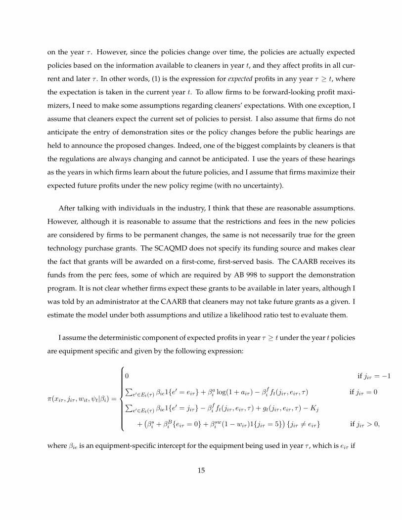
I assume the deterministic component of expected profits in year τ ≥ t under the year t policies

are equipment specific and given by the following expression:

π(xiτ , jiτ , wit, ψt|βi) =

0 if jiτ = −1∑e′∈Et(τ) βie1{e

′ = eiτ}+ βai log(1 + aiτ )− βfi ft(jiτ , eiτ , τ) if jiτ = 0∑e′∈Et(τ) βie1{e

′ = jiτ} − βfi ft(jiτ , eiτ , τ) + gt(jiτ , eiτ , τ)−Kj

+(βsi + βBi {eiτ = 0}+ βswi (1− wiτ )1{jiτ = 5}

){jiτ 6= eiτ} if jiτ > 0,

(4)

where βie is an equipment-specific intercept for the equipment being used in year τ , which is eiτ if

15

the cleaner does not purchase new equipment and jiτ otherwise. The profit function when firms

use their existing equipment depends on the equipment age, reflecting maintenance costs and/or

expected losses from machine failure associated with using older equipment but not with new

equipment. I assume age enters through a concave function to allow for rapid initial declines

in value (which is consistent with secondary market values for durable goods). As a robustness

check, I allowed age to enter in a more flexible manner, but I found the same, concave effect so I

report the results using the log specification.20 Note that the age coefficient reflects the value of

using existing equipment relative to the scrap value, which I normalize to zero, so if scrap value

also depends on age, we would expect the age coefficient to be smaller in magnitude. 21

Again, ft(jiτ , eiτ , τ) are the announced solvent fees for equipment eiτ at time τ (perc is the only

taxed solvent in California) and gt(jiτ , eiτ , τ) are the equipment grants, which reduce the capital

costs Ke22 when the cleaners purchase new equipment. The units are in $10,000, and the perc

fees are the fees per 46,600 pounds of clothes cleaned, the average annual amount by one cleaner.

Without loss of generalizability, I normalize the coefficient on the equipment costs to be equal to

one; this leads to a direct interpretation of the coefficients in their monetary equivalents. Since the

equipment costs and fees must lead to lower profits, I include negative signs for these terms. I

constrain the fee parameter to be positive by estimating its log. βB capture barriers to entry for

new entrants.

The last term in the profit function when cleaners purchase new equipment captures state

dependence. I allow for there to be learning costs if the cleaner is switching to a different type of

technology. In addition, in the case of wet cleaning, I allow there to be additional switching costs

due to the complexity in the wet cleaning process and the differences from the other cleaning

methods. This is where I allow the demonstration sites to have an effect. I assume that these20I also tried allowing equipment age to enter into the profit function when purchasing new equipment since there

may be age-dependent scrap value which differs from that when exiting the market, but I found this coefficient to beimprecisely estimated and close to zero.

21After 2003, firms with perc equipment older than 15 years old have to discontinue use of the equipment. I do notalways observe these firms immediately exit the market or buy new equipment, so I allow for this small minority offirms to remain in the market with profits equal to an estimated intercept. These firms may be outsourcing the cleaningor actually be inactive, waiting to purchase new equipment in a later year, and I do not attempt to distinguish betweenthe two.

22I use known average equipment costs for Ke, as reported in the 2006 CAARB report shown in Table 2. The equip-ment cost data excluding grants are therefore time invariant. This is not an issue since the size of the grants greatlyexceeds the actual changes in equipment costs over the period of study.

16

additional costs when switching to wet cleaning are eliminated for the incumbent cleaner if it has

visited a demonstration site, indicated by sit, in which case the switching costs are the same as for

any of the other types of equipment.23

4.2 Value Function Computation

I solve for the value function explicitly. Cleaners’ total expected profits are calculated by summing

up the expected current and discounted future profits:

V (xit, ψt, wit|βi) =∑∞

τ=t ρτ−tExiτ ,εijτ

[maxjiτ∈Ct(τ) [π(xiτ , jiτ , ψt, wit|βi) + σiεijτ ]

](5)

= Eεijt[maxjit∈Ct(t+1) V (xit, jit, ψt, wit|β) + σiεijt

].

where V (·) is the choice-specific value function. The cleaner chooses the choice j that maximizes

total expected profits. The future states and choices will depend on the realization of the stochastic

terms. The time subscript on ψ and s on the right hand side is t since the policies in future years

are expected to be the same as the current announced policies, and the cleaners are assumed to

not anticipate more demonstrations in future years. I can write the choice-specific value function

using the following Bellman equation:

V (xit, ψt, wit|βi) = π(xit, ψt, wit|βi) + ρEεijt+1

[max

j ′∈Ct (t+1 )

[V (xijt+1 , jijt+1 , ψt ,wit |βi) + σiεijt+1

]],

(6)

where ρ is the discount factor and the state at t + 1 is deterministic conditional on εijt+1 and the

current state and choice at time t. In the years before the state regulations began in late 2002

and after the 2020 phase-out, the market is in a stationary equilibrium and can be computed as

the fixed point solution to the Bellman equation. In the years after the state regulations began

2002 and before the 2020 phase-out, the market is non-stationary and I use 6 to calculate the non-

stationary value functions for every year between 2003 and 2020, working backwards from my

23I assume that potential entrants already have the information and training that is acquired by visiting a demon-stration site i.e. viτ = 1 since it is likely they are well informed regarding the use of the new technologies. By usingsit instead of siτ , I implicitly make the assumption that cleaners do not factor in their ability to attend future demon-strations, reasonable since there was no indication that the demonstrations would continue. Relaxing this assumptionwould require me to estimate an additional demonstration model.

17

fixed point solution for the value function in 2021 and thereafter.

I have to recompute both stationary value functions (pre-2003 and post-2020) as well as the

non-stationary value functions every time a policy change occurs in the data. Before any policies

are announced, cleaners’ stationary value functions for all years are those calculated for the pre-

regulation period since the cleaners do not anticipate the future regulations. The value functions

are different in 2003 when the policies are first announced. In the aforementioned example, before

it was announced in January 2007 that no sales of perc machines for use in California would be

allowed after 2007, firms expected that they would be able to continue to buy perc machinery until

2020 and the value functions were computed under these expectations. Firms’ value functions

in 2006 were quite different than in 2007 when firms’ expectations changed as a result of this

newly announced regulation change. Although this adds to the computational complexity, these

changes in the policies are what allow us to estimate the discount rate by providing the necessary

exclusions restrictions.

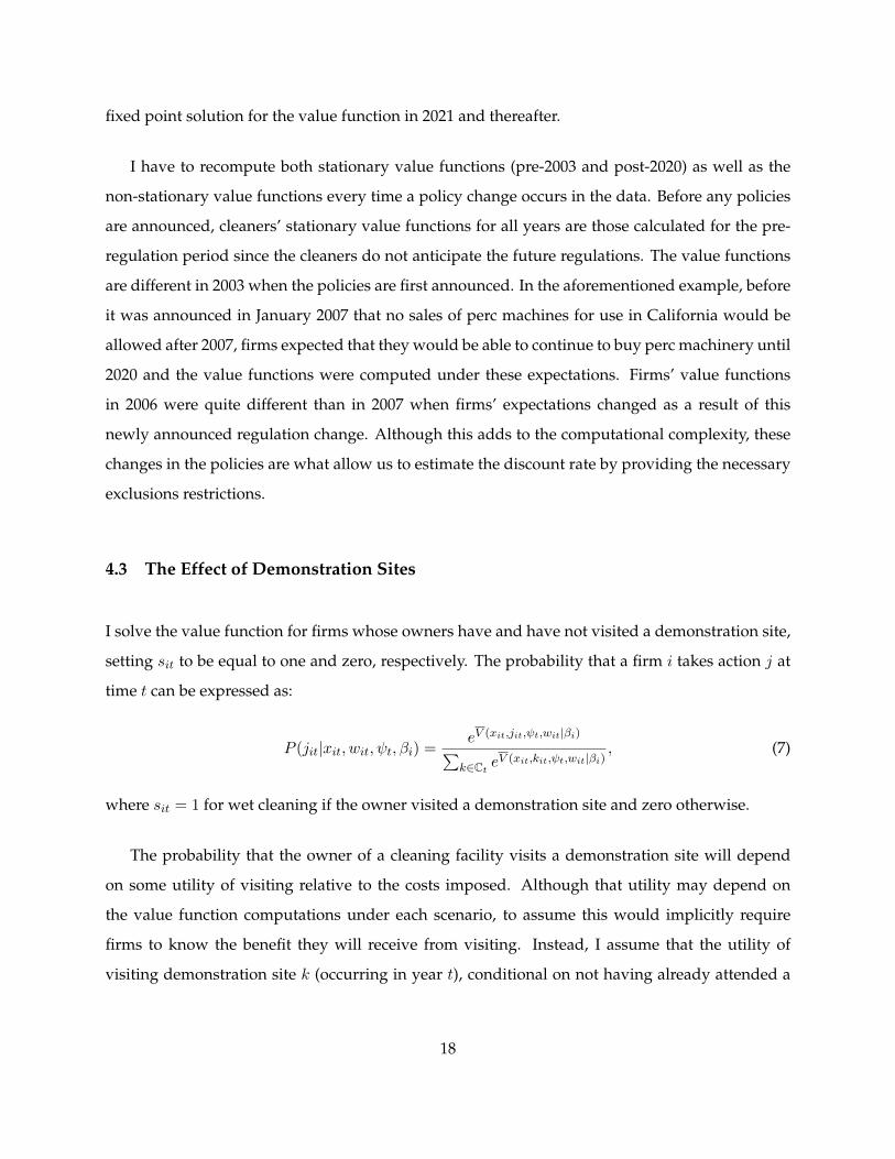
4.3 The Effect of Demonstration Sites

I solve the value function for firms whose owners have and have not visited a demonstration site,

setting sit to be equal to one and zero, respectively. The probability that a firm i takes action j at

time t can be expressed as:

P (jit|xit, wit, ψt, βi) =eV (xit,jit,ψt,wit|βi)∑

k∈Ct eV (xit,kit,ψt,wit|βi)

, (7)

where sit = 1 for wet cleaning if the owner visited a demonstration site and zero otherwise.

The probability that the owner of a cleaning facility visits a demonstration site will depend

on some utility of visiting relative to the costs imposed. Although that utility may depend on

the value function computations under each scenario, to assume this would implicitly require

firms to know the benefit they will receive from visiting. Instead, I assume that the utility of

visiting demonstration site k (occurring in year t), conditional on not having already attended a

18

demonstration, takes the following reduced form function of the state variables:

Uwkt(xit, ψt|βi) = γeeit + γaait + γddik + γ20081{t = 2008}+ γ20091{t = 2009}+ ηit, (8)

where dik is the distance to the demonstration site and ηit is assumed to follow a standard iid type

1 extreme value distribution. This specification allows firms’ decisions to visit to be a function

of the state variables but does not impose the assumption that cleaners can anticipate the benefit

they will receive from visiting. In addition to annual shocks in attendance costs, any changes in

the option value of waiting for future demonstrations are captured in the year dummy variables –

if firms believe there will be future demonstrations, this will lead to lower current probabilities of

visiting, and by including year dummies, we allow such beliefs to change. Due to data limitations,

I restrict γe to be the same for cleaners who currently have wet cleaning, carbon dioxide cleaning,

or GreenEarth cleaning.

The probability of attending demonstration k (which occurs in year t) if the cleaner has not

already attended one is given by:

Pwik =eU

wkt(xit,ψt|βi)

1 + eUwkt(xit,ψt|βi)

.

I assume that once a cleaner visits a demonstration, they will visit another with zero probability

since they receive no additional benefit.

I recursively define P̃wik , the probability that the owner of a cleaner has visited at least one

demonstration site immediately after demonstration k occurs:

P̃wik =

P̃wi(k−1)(1−Wik) +Wik) if k ∈ KW

P̃wi(k−1) + (1− P̃wi(k−1))Pwik , otherwise

(9)

P̃wi0 = 0.

where Wik if the realized attendance decision and KW is the set of k for which these data are

available.

19

For the demonstrations for which I have attendance data, the realized values (zeros or ones)

are used in expression (9) in calculating the probabilities of visiting later demonstrations. This

means that if we observe that a cleaner has attended a demonstration, the probabilities of visiting

later demonstrations are zero. The probability a cleaner has visited at least one demonstration site

by the end of year t is then given by:

P̃wit = P̃wikt , (10)

where kt is the last demonstration in year t. Once a cleaner is observed to have visited a demon-

stration, say demonstration k, P̃wik′t = 1 for all later demonstrations k′ > k.

This formulation of how demonstration sites affect profits has a couple of desirable features.

First, by letting a demonstration site affect firm profits in the current and later periods, I allow

for owners to attend a demonstration in one year to acquire information and training in the use

of wet cleaning, and their profits will be affected if they then switch to wet cleaning in a later

year. Although this could have been done by including the distance to the nearest demonstration

site as another observable state variable that directly enters profits, my implementation is more

realistic. The owner of a cleaner either will or will not visit each demonstration site, depending on

the distance to the demonstration site. The farther the demonstration site, the less likely an owner

will be aware of it or able to make the trip, but the benefit from visiting should not not depend on

the distance.

The probability that firm i takes action j at time t can now be expressed as the sum of the

choice probabilities conditional on having visited or not visited a demonstration site, multiplied

by the probability that the firm owner did or did not visit a demonstration site:

P (jit|xit, ψt, βi) = P (jit|xit, wit = 1, ψt, βi)P̃wit + P (jit|xit, wit = 0, ψt, βi)(1− P̃wit ). (11)

4.4 Estimation

I first estimate the attendance parameters in a first stage using maximum likelihood estimation.The

likelihood of the attendance data is the product of the unconditional probabilities of attending and

20

not attending each demonstration k for which I have attendance data:

LW =I∏i=1

∏k∈Kw

((1− P̃wi(k−1)t

)Pwikt

)Wikt(P̃wi(k−1)t +

(1− P̃wi(k−1)t

)(1− Pwikt)

)1−Wikt

, (12)

I estimate these γ coefficients in a first stage and then use the fitted values in the second stage

when the attendance data are not available.24

I first estimate the choice model under the assumption of homogenous firms, setting the annual

discount factor at ρ = 0.9. Let a firm’s observed actions at time t be given by Yit and state by Xit.

The likelihood of all cleaners’ actions (incumbents and potential entrants) conditional on β can be

expressed as:

L(Y |X,β) =I∏i=1

T∏t=1

P (Yit|Xit, ψt, β), (13)

where the capital letters indicate observed data and I is the total number of incumbent firms and

potential entrants. I assume that in any year, there are 300 potential entrants, approximately 1/10

of the number of incumbent firms. I assume that these firms can only enter the market in the

current year, and are replaced by 300 different potential entrants in the next year. The likelihood

expression includes the probability that the new entrants enter and that three hundred minus

the number of actual new entrants in each year choose to not enter the market, as well as the

probabilities of all of the incumbents’ actions. By including potential entrants in the likelihood

function, I allow for the endogenous entry of cleaners in the model of technology adoption. The

choice of the number of potential entrants will determine the estimate of the entry costs but should

not appreciably affect the estimates of the other parameters.

When including firm heterogeneity, the likelihood of cleaner i’s actions conditional on βi is

given by:

Li(Yi|Xi, βi) =

T∏t=1

P (Yit|Xit, ψt, βi). (14)

24Alternatively, I could estimate the γ coefficients jointly when estimating the model of equipment choice; however,this is not possible when including firm heterogeneity. Since cleaners only visit a demonstration once, I effectivelydo not have a panel of observations for the decision to visit and so cannot identify heterogeneity in the decision toattend a demonstration. Because my estimation method for the profit parameters includes heterogeneity in all of theparameters, it is necessary to estimate the homogenous demonstration site visitation parameters in a first stage.

21

To determine the unconditional likelihood for cleaner i, I need to integrate over the distribution of

βi for observed cleaners:

Li(Yi|Xi) =

∫ T∏t=1

P (Yit|Xit, ψt, βi)dF̂ (βi), (15)

where F̂ (βi) is the cumulative probability distribution of βi for firms in the market. I assume that

the distribution of βi for potential garment cleaners follows a multivariate normal distribution:

βi ∼ N(Ziθ,Σ), (16)

where θ and Σ are parameters to be estimated and Zi includes exogenous, time-invariant demo-

graphic demand variables and firm variables which explain some of the heterogeneity.

This distribution is not the same as the empirical distribution of parameters for firms in the

data. It is necessary to control for the sample selection: Cleaners with more favorable profit pa-

rameters are more likely to be in the data. The distribution f̂(βi) is equal to the probability that

cleaner i has profit parameter vector βi and is in the panel data at time t = 0, which is equal to the

following:

f̂(βi) = P (Xi0, βi) = p(Xi0|βi)f(βi|Ziθ,Σ), (17)

where f is the probability distribution function for potential garment cleaning firms. The tradi-

tional challenge in controlling for the initial conditions (at t0 = 1999) is the calculation of p(Xi0|βi).

However, I can calculate the stationary probability distribution of the state variables at the start

of my panel p(Xi0|βi) by iteratively multiplying the state transition matrix by itself until the so-

lution converges, for every draw of βir. The deterministic state transition matrix is equal to the

state transition matrix conditional on the firm’s actions multiplied by the probability of the firm’s

actions, which are conditional on the state Xit and parameter vector βi:

P (x′i|xi, ψ1999, βi) = P (x′i|xi, j)P (j|xi, ψ1999, βi) (18)

P (xi0|βi) = P (x′i|xi, ψ1999, βi)∞.

22

Maximizing the simulated log likelihood function with standard numerical integration would

involve drawing from the distribution of βi and recomputing the value functions for all states and

draws every iteration of the optimization process. To alleviate the computational burden, I instead

use a change of variables method and importance sampling to evaluate the integral as described

in Ackerberg (2009). The insight of importance sampling is that it is only necessary to compute the

value functions and individual likelihoods once, for each draw of the parameter vector. Instead

of changing the simulation draws for each iteration of the optimization process, which are given

equal weight in evaluating the integral using traditional numerical integration, for each individual

I use the same set of draws throughout optimization and simply change the weights on each of

the R draws by maximizing the likelihood function over the parameters of the distribution of βi.

In practice I use four different sets of draws, evenly allocating firms across the sets, which is why

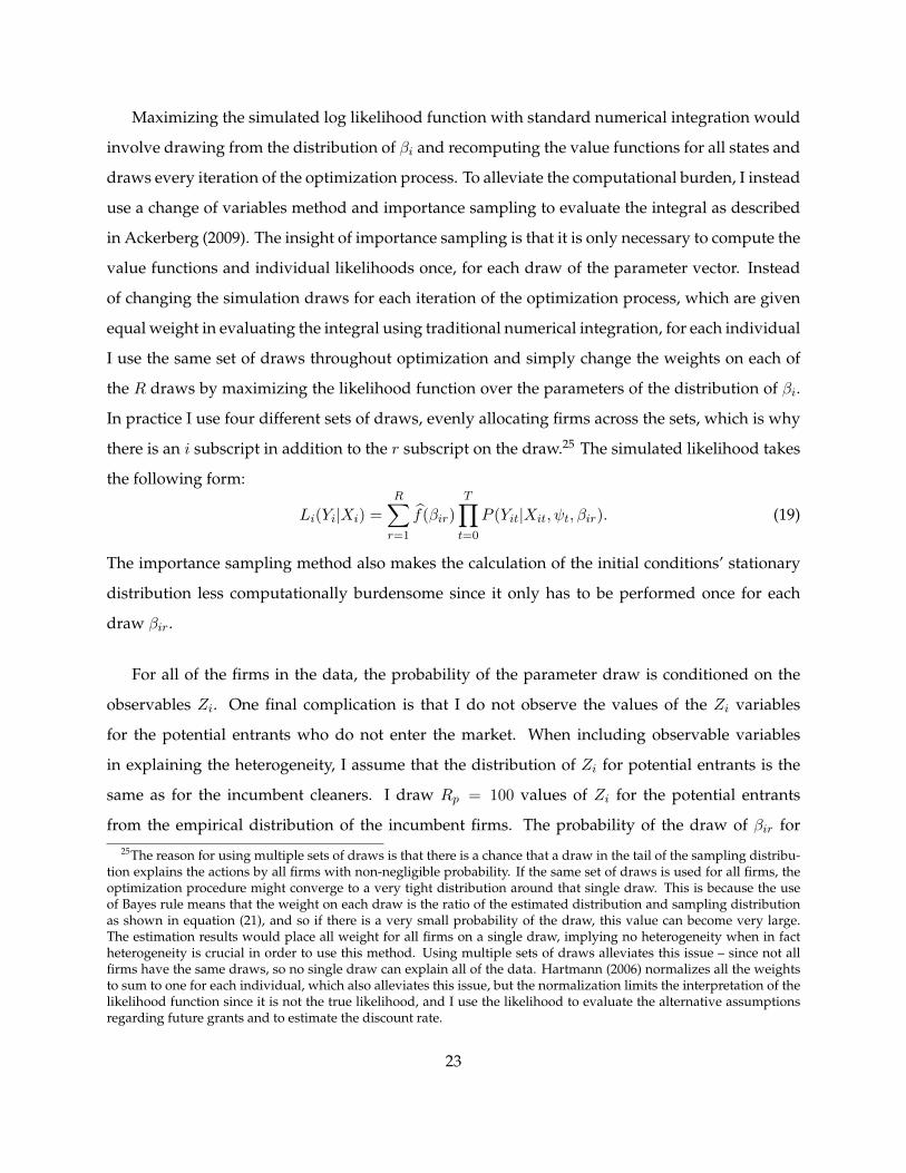
there is an i subscript in addition to the r subscript on the draw.25 The simulated likelihood takes

the following form:

Li(Yi|Xi) =

R∑r=1

f̂(βir)

T∏t=0

P (Yit|Xit, ψt, βir). (19)

The importance sampling method also makes the calculation of the initial conditions’ stationary

distribution less computationally burdensome since it only has to be performed once for each

draw βir.

For all of the firms in the data, the probability of the parameter draw is conditioned on the

observables Zi. One final complication is that I do not observe the values of the Zi variables

for the potential entrants who do not enter the market. When including observable variables

in explaining the heterogeneity, I assume that the distribution of Zi for potential entrants is the

same as for the incumbent cleaners. I draw Rp = 100 values of Zi for the potential entrants

from the empirical distribution of the incumbent firms. The probability of the draw of βir for25The reason for using multiple sets of draws is that there is a chance that a draw in the tail of the sampling distribu-

tion explains the actions by all firms with non-negligible probability. If the same set of draws is used for all firms, theoptimization procedure might converge to a very tight distribution around that single draw. This is because the useof Bayes rule means that the weight on each draw is the ratio of the estimated distribution and sampling distributionas shown in equation (21), and so if there is a very small probability of the draw, this value can become very large.The estimation results would place all weight for all firms on a single draw, implying no heterogeneity when in factheterogeneity is crucial in order to use this method. Using multiple sets of draws alleviates this issue – since not allfirms have the same draws, so no single draw can explain all of the data. Hartmann (2006) normalizes all the weightsto sum to one for each individual, which also alleviates this issue, but the normalization limits the interpretation of thelikelihood function since it is not the true likelihood, and I use the likelihood to evaluate the alternative assumptionsregarding future grants and to estimate the discount rate.

23

the potential entrants who do not enter is calculated by numerically integrating over these Zi,

f(βir) = 1Rp

∑Rprp=1 f(βir|Zrp).

For notational convenience, I define P (Xi0|βir) = 1 for those cleaners who are not present in

the data set at the beginning of the panel. The likelihood of the data can now be written as:

L =I∏i=1

R∑r=1

wirP (Xi0|βir)T∏t=0

P (Yit|Xit, ψt;βir), (20)

where the weights for each draw are the product of the probability of the draw multiplied by the

probability that that draw would be present in the data prior to the beginning of the panel at t = 0,

for those cleaners who are present at the beginning of the panel. The values of w are equal to the

ratio of the probability distribution functions f(.) and the sampling distribution f0(.):

wir =f(βir|Ziθ,Σ)

f0(βir|θ0,Σ0). (21)

I estimate the model by maximizing the log likelihood over the parameters θ and Σ.

As previously mentioned, I assume that firms expect the current policies to continue according

to the description within the regulation. For example, when the phase-out of perc was announced

for 2020, cleaners proceeded under the assumption that this indeed would be the case. The policy

tool that is accompanied by more ambiguous expectations is the green equipment grants. I esti-

mate the model under two alternative assumptions: First, that cleaners expect the green equip-

ment incentives to be available in future years, and second, that they expect the incentives to be

available only for the current year.

For the heterogeneous model, in addition to estimating the profit function parameters, I esti-

mate a homogenous discount rate by performing a grid search over discount rates between 0.7

and 0.95 in increments of 0.01, using R = 10, 000. I do this under both assumptions on the avail-

ability of future grants. 26 I then rerun the estimation with the estimated discount factor, using

these parameter estimates as the parameters of the new sampling distribution, multiplying the

26I use a normal distribution for the sampling distribution, using rounded estimates from a previous estimation withρ = 0.9 as the mean of the sampling distribution, and the identity matrix multiplied by a scale factor of four as thecovariance matrix to ensure sufficient coverage of the parameter space.

24

variance matrix by a scale factor of four. I use R = 25, 000 and estimate the model with 15 differ-

ent bootstrap samples (randomly sampling cleaners) using a different set of parameter draws for

each bootstrap sample to get estimates of the standard errors which incorporate the simulation

error.

4.5 Identification

Identification of the model parameters is dependent on what actions the cleaners have made in

which states. As previously mentioned, I observe cleaners enter, make the choice to buy new

equipment, operate using their existing equipment, and leave the market, but almost no cleaners

who adopt wet cleaning, carbon dioxide, or GreenEarth equipment then exit the market or pur-

chase new equipment in a later year. For this reason, I cannot separately identify utilization utility

from purchase utility for each type of equipment; I instead include the average equipment costs

found in the 2006 CAARB report.

The timing of firms exiting the market and purchasing new equipment allows me to identify

the effect of equipment age on a firm’s utility in each period both when using existing equip-

ment and purchasing new equipment. In addition, I can identify utility intercepts for each type

of technology I observe being purchased in the data. To separately identify purchase and utiliza-

tion intercepts, I need to observe firms with each type of equipment make subsequent purchase

decisions in 2001 or later, which is not the case. To address this issue, I include observable average

equipment costs for the different types of equipment. I normalize the effect of equipment costs to

be one which allows me to estimate the standard deviation of the stochastic term. Identification of

the perc fee coefficient is possible from the time-series variation in the perc fees, which begin at $3

per gallon of perc in 2004 and increase annually by one dollar to a maximum of $12 in 2013 (this

was known to firms in 2003). I can get identification from the different behavior of firms in these

years as well as the fact that there were no announced fees before 2003.

The state dependence coefficients are possible to identify because of the presence of new en-

trants in the data. Because new entrants do not experience the same switching costs as incumbent

25

firms (since they have no current equipment), the differences in the purchases by incumbents and

new entrants provides the necessary cross-sectional variation to identify the switching cost coef-

ficient which by assumption is the same for all equipment types. The model includes additional

switching costs when firms purchase the more complicated wet cleaning equipment and have not

attended a demonstration, and this coefficient is identified from the differences in behavior by

firms who have and have not visited a wet cleaning demonstration. The γ coefficients determin-

ing visitation are identified with the attendance data and from variation in cleaners’ geographic

proximity to the different demonstration sites. The entry costs for the new entrants (which in-

cludes learning costs) is identified, after specifying a number of potential entrants each period, by

the number that actually enter.

The identification of firm heterogeneity is possible due to the panel structure of the data, but

it is aided by the changing regulations and incentives. With every policy change, the relative

utilities of firm choices are changed, leading to different probabilities for each choice alternative.

The choices different firms make as functions of their states and the current policies not only

allow me to better identify the heterogeneity, but to identify the discount rate. Since two of the

polices directly alter future profits but do not affect current period profits (the ban on perc use

after 2020 and the later ban on perc equipment purchase after 2007), I have the necessary exclusion

restriction.

5 Results

I begin by estimating the model of demonstration site visitation; the results are shown in Table

10. I find that cleaners are more likely to visit a demonstration site if they currently use a green

technology other than hydrocarbon. Surprisingly, equipment age has a negative impact on the

decision to visit. Cleaners are less likely to visit demonstrations in later years, and as we would

expect, the farther the demonstration site, the less likely a cleaner is to attend.

I first estimate the choice model with firm profits given in (4), assuming homogenous firms,

under the alternative assumptions that firms expect and do not expect the grants to be available

26

in future years. I constrain the coefficients on the perc fees to be positive by estimating the log of

the parameter, which leads to a negative effect of fees on profits; I also constrain σ to be positive

in the same manner. The results are shown in Table 11. The age coefficient is negative as expected

under both assumptions. Under both assumptions regarding future green equipment grants, the

results indicate that the carbon dioxide technology is the most profitable, followed by perc and

hydrocarbon, Green Earth, and wet cleaning last.27

The relative profits when using the different types of equipment are not surprising given the

overall adoption of the different types of technology and the differences in equipment costs. The

lack of widespread adoption of wet cleaning in particular, considering there may actually be cost

benefits, points to industry skepticism. Although the CAARB has conducted efficacy tests for wet

cleaning and found that over 99.5 percent of the garments that are usually dry cleaned are able to

be wet cleaned, this does not mean that the owners of cleaning establishments are convinced that

wet cleaning is a sufficient substitute for traditional dry cleaning. I have spoken with individuals

in the industry who conveyed doubts regarding the efficacy of wet cleaning, and cleaners using

wet cleaning will sometimes outsource some garments to traditional perc facilities. The results

support this hypothesis – switching costs are significant and are higher for wet cleaning if the

cleaner has not visited a demonstration site.

These results of course ignore heterogeneity across cleaners in profitability when using the dif-

ferent types of equipment. The full model includes heterogeneity in all of the firm profit param-

eters. As described earlier, firm heterogeneity is included with the use of importance sampling,

where I draw the parameters from a multivariate normal distribution.28 I estimate the mean and

covariance matrix of the multivariate normal distribution from which the parameters are drawn.

Again, I constrain both the coefficient on the perc fees and σ to be positive by estimating the log

of the parameter. This means that these two parameters are distributed log normal. I estimate the

model this way to ensure that the values of the parameters in the tails of the distributions do not

27Under the assumption that cleaners do not anticipate future grants, I estimate all equipment profits to be slightlyhigher, the perc fee has less of an effect, and switching costs are lower. All of these factors would indicate that thereare slightly higher period profits for all technologies. This is as expected since without the grants, the option value forbuying green equipment is lower and so higher current profits are needed to explain the observed level of adoption.

28Although in theory I can estimate some of the off-diagonal elements of the covariance matrix, data limitationsprevent this in practice.

27

lead to implausible predictions, such as profits that increase with higher fees.

As with the homogenous model, the parameters are estimated under the competing assump-

tions that firms expect the green technology incentives to be present for only the current year or

both the current and future years, in conjunction with a grid search over discount rates. I plot

the log likelihood in Figure 4 as a function of discount rate under both assumptions regarding

future grants. The assumption that cleaners do not expect future grants is preferred accoring to

the Bayesian Information Criterion which permits tests of non-nested models.29. As previously

described, the model is re-estimated using these first stage estimates as basis for the new sam-

pling distribution (using the estimated mean and four times the estimated covariance), using the

0.89 discount rate and assuming that firms do not expect the grants to be available in future years.

Table 11 shows the estimation results averaged over fifteen sets of simulations; I find that the

simulation error dominates the estimates of the asymptotic standard error and so I report the sim-

ulation error in the table. Because of my normalization, the coefficients for the different types of

equipment can be interpreted as dollar amounts (measured in units of $10,000); for example, perc

cleaning yields $7,630 dollars in annual profits.

When allowing for firm heterogeneity, the relative average profitability of the technologies is

the same as in the homogenous case – however, with the exception of hydrocarbon, the green

technologies all exhibit significantly higher variance in their profitability across firms. This is es-

pecially true for wet cleaning, which has a large, negative profitability for the average cleaner

but exhibits the highest variance in cleaner profits when using this technology. This finding has

important implications for the future adoption of the technology; unless these profits can be im-

proved, wet cleaning is unlikely to exhibit large market penetration, even with its lower operating

costs and with high subsidies. None of the technologies lead to high profit margins, consistent

with anecdotal evidence.

Since the coefficient on the perc fee is distributed log normal, the mean effect of the fee is

exp(0.570 + 0.2502/2) = 1.824, so the average effect of the fee in per-dollar terms is 82% larger

than the equipment grants. This may be due to the fact that the equipment may be financed.

29The test statistic is twice the difference in the log likelihoods at their maximums, equal to 166 at ρ = 0.89, minuspenalty terms for the number of parameters which is the same under both sets of assumptions.

28

One implication is that manufacturers of the green (or perc) equipment may find it profitable to

subsidize solvent costs. The high variance in the effect of the per-gallon perc fee is likely due to

variance in the volume of clothes cleaned by the different cleaners.

The switching cost parameters are also both negative, indicating that firms do exhibit state de-

pendence in their equipment choice, and they are even less willing to switch to wet cleaning un-

less they have visited a demonstration site. The barrier to entry intercept is negative as expected,

although the barrier to entry is identifiable only by specifying a priori the number of potential

entrants.

The large amount of heterogeneity is hardly surprising. It is reasonable to expect that different

firms would make different profits using different types of equipment. Accounting for this hetero-

geneity is crucial in accurately forecasting the adoption of the perc alternatives. To try to explain

some of the heterogeneity in firm profits, I estimate the model including market demographic

variables as shifters of the parameter means. The zip-code level demographic variables are in-

tended to capture consumer demand shifters for garment cleaning, or environmentally friendly

cleaning specifically, and include median income, average household size, the fraction of vehicles

registrations from 2001-2008 which are hybrids, and the fraction of the population who are male,

white, aged 20-44, aged 45-64, unemployed, have a college degree, and use clean transit to com-

mute to work. In general the coefficient estimates are not significant for any of these variables in

explaining the heterogeneity in firms’ profit parameters. I perform the estimation with just zip

code population density and hybrid registrations, with the same results. One explanation is that

the limitations of the data (no price and quantity information, infrequent firm actions) prevent

precise estimation of these effects.

5.1 Robustness Checks

To model the probability a cleaner visits a demonstration site, I used a reduced-form expression for

the utility from visiting. Alternatively, I could assume that the value of visiting a demonstration,

conditional on not yet attending one, is equal to the difference in the conditional value functions

29

given in (6) for s = 0 and s = 1, so that

Uwkt(xit, ψt|βi) = V (xit, ψt, wit = 1|βi)− V (xit, ψt, wit = 0|βi) + γddik + ηit. (22)

The implicit assumption in this specification is that cleaners know the size of the extra switching

costs for wet cleaning that can be eliminated by attending a demonstration. Although this is a

questionable assumption, I still estimated the model using this more structured approach to esti-

mate the probabilities of attending a demonstration; the results on the profit function parameter

estimates are minimal.

One assumption needed to estimate the entry costs was the number of potential entrants. Al-

though changing the number of potential entrants does lead to different estimates of the entry

costs, the other parameter estimates are largely unchanged. As previously mentioned, I did use

more flexible specifications for the effect of equipment age as well, but found that the estimated

coefficients led to a function similarly shaped to the concave logarithmic function. Although in

theory it is possible to allow the effect of equipment age of the existing equipment to enter when

purchasing new equipment, I found the estimated coefficient to be imprecisely estimated and

close to zero, indicating that any age-dependent scrap value for the old equipment when purchas-

ing new equipment is about the same as when exiting the market.

One potential concern is endogeneity of the demonstration sites. For this to be an issue, clean-

ers electing to be demonstration sites would need to be disproportionately represented in areas

where cleaners are more likely to purchase wet cleaning equipment. I do find correlation in the

green profit parameters and the effect of the demonstrations in alleviating the additional wet

cleaning switching costs. However, if the demonstration locations are endogenous, this would

impact the estimate of the effect of distance to the sites, but should not significantly impact the

state dependence parameter measuring the effect of the sites, which is primarily identified using

actual attendance data.

To further assess the endogeneity concern, I estimated the base model with heterogeneity using

fit values of the distances to demonstration sites variables, regressing the distances on exogenous

instruments. For instruments, I used a dummy variable indicating if the zip code is a low-income,

30

cancer risk area where there was extra effort to get cleaners to become demonstration sites, as

well as the number of total dry cleaners within a five kilometer radius, since most demonstration

sites are cleaners and a high number of nearby cleaners increases the probability of one becoming

a demonstration site. Although one could anticipate cleaners being reluctant to share the infor-

mation with their competitors, I have found that cleaners actually welcome the chance to share

their knowledge by speaking at educational meetings, and they are compensated for becoming

a demonstration site. The results using the fitted distance variable are similar to those using the

actual distances for the other coefficient values.

6 Discussion

Because of both the durable nature of the equipment and the changing incentives and regulations,

it is necessary to account for possible state dependence in cleaners’ adoption decisions, both on

current equipment type and age, as well as on the current year. I find that the average effect of

equipment age does lead to lower profits when using existing equipment, likely due to increased

maintenance costs. I find a non-negligible effect of the demonstration sites in reducing switching

costs to wet cleaning which varies considerably by cleaner, and the magnitude of these switching

costs are positively correlated with profits when using one of the green technologies. Not surpris-

ingly, New York and Massachusetts are also implementing demonstration site programs to help

increase adoption of green cleaning technologies.

In addition to the effectiveness of the demonstration sites, I find that the effect of the perc fees is

larger than that of the equipment purchase grants, possibly since the equipment can be financed.

I model equipment costs as up-front costs. If firms finance the equipment and discount future

profits more than their interest rate, then the value to cleaners of changes in capital expenditures

due to grants would be less than changes in fees which affect current profits only. The implica-

tion is that manufacturers of the alternative technologies should not only supply information and

training to garment cleaners, they may also want to subsidize the alternative solvents, even if this

means that the equipment costs would be higher.30

30Equipment manufacturers are trying to help provide the information to cleaners from their presence at informa-

31

The heterogeneity in the profit parameters can be explained either through cost differences,

volume heterogeneity, or through prices. It may be the case that garment cleaning firms have the

ability to differentiate themselves along an environmental dimension. One limitation of the model

used in this paper is that it does not account for strategic behavior by firms in the timing of adop-

tion of new technologies. However, I did not find any evidence that firms are strategic in their

adoption decisions; if they are, then it is likely a second order effect in comparison to the effect of

the state variables and policies. This is not surprising, since the policies in California have been

changing so much that cleaners are having enough trouble keeping current on the restrictions and

incentives. In talking with the owners of cleaning establishments and from questions posed at

a cleaning information session sponsored by the San Francisco Department of the Environment,

owners were far more interested and worried about constantly changing and unanticipated reg-

ulations, and the efficacy of the new technologies than they were about how consumers would

react to the use of the new technologies.

That being said, there may still be a significant portion of consumers who would be willing

to pay for cleaner technologies. Unfortunately, although there has been a great deal of effort to

educate the owners of cleaning establishments about the perc cleaning alternatives, consumers for

the most part are not informed about these alternatives and there exists no control or oversight re-

garding environmental claims by cleaners. Some cleaners do change their names after purchasing

one of the cleaner technologies, and the word ”organic” appears often in the windows of cleaners,

but it is a meaningless term. All organic means in the context of garment cleaning is that carbon-

based chemicals are used, which include perc. Because of the lack of consumer education and no

oversight of environmental claims, it is up to consumers to figure out which cleaners actually use

environmentally friendly technologies.

If there was more certainty in the future regulations as well as consumer education and over-

sight of the environmental claims made by cleaners, then there would be the potential for com-

petitive advantages in adopting a green cleaning technology. The current system makes it very

hard for firms using the clean technologies to convey that information to consumers. The Green

Cleaning Council was recently established in 2008, with the help of the National Cleaners Asso-

tional sessions on the use of the new technologies sponsored by the different air quality management districts in thestate and by the CAARB, along with the San Francisco Department of the Environment and other local organizations.

32

ciation, to help provide information to consumers and to provide an environmental rating sys-

tem for garment cleaners. This may help, but the rating system is voluntary and relies on the

statements made by individual businesses. A reliable, non-voluntary third party verification and

rating system could help allow consumers to make educated choices between cleaners based on

their environmental commitment, which could be an alternative way to increase green technology

adoption without relying solely on grants, fees and restrictions.

7 Counterfactual Analysis

7.1 Policy Effects on Adoption

The benefit of California’s multi-pronged approach to phase out perc and favor carbon dioxide

and wet cleaning, from a research perspective, is my ability to separately identify the benefits of

each policy tool used. In this section, I perform counterfactual analyses using simulation to predict

the future state of the southern California garment cleaning industry for different combinations

of policy tools. In this way, I assess the relative impact of the different tools on green technology

adoption. I begin the simulations using the 2002 cleaners, so the first year of the simulation is

2003, when the California policies began.

Figure 5 shows the results of the simulations using all of the policy tools, with the exception

of the demonstration sites, and also each tool used separately. As expected, California’s multi-

pronged approach of fees, grants and strict regulation lead to higher initial adoption of green

technologies than any one policy tool in isolation, although the both the multi-pronged approach

and the strict regulation both lead to 100% adoption by the end of 2020, by necessity. The grants

lead to less green technology adoption than the fees, as expected since on a per-dollar bases, the

fees are actually more effective. Without the strict regulation, adoption of the green technologies

always flattens out below 25%: At 21% with grants, 23% with fees, and 19% with no policy. About

a third of firms have adopted the green technologies by the end 2009 in the simulation, which is

agreement with the actual fraction seen in the data.

33

Figure 6 shows the effect of the demonstration sites, plotting the relative difference in the

number of cleaners using each type of technology with and without demonstrations (under Cal-

ifornia’s multi-pronged policy approach). Again, the simulations with demonstrations assume

that all firms receive the benefit of the demonstrations. In this situation, I find an increase in the

number of cleaners using wet cleaning of 35%, although this is accompanied by a slight decrease

in the number of cleaners using the other green alternatives. The number of cleaners using perc

drops by 3.5% by 2020 as a result of the demonstration sites. Since all cleaners ultimately adopt

green technologies under the California polices, the two main benefits of the demonstrations in re-

ducing perc use is the acceleration of the process, and the small increase in the number of cleaners

who decide to remain in the market as a result.

Although the effectiveness of the strict regulation is attractive, it must be weighed against the

effect on firm entry and exit. Figure 7 plots the simulated number of firms in the market under

the same set of policy alternatives (with no demonstrations). Under the multi-pronged approach

which causes the most net exit, the number of expected firms in the market will shrink to 65%

of the number under no policy, and under just the strict regulation, the number shrinks to 77%.

Although the strict regulation is highly effective in getting cleaners to switch technologies, by

removing the ability of firms to use perc, many firms will ultimately exit the market. The removal

of the option value of purchasing perc after 2007 leads to an acceleration in the number of firms

exiting the market beginning this year when the policy was announced. To assess the resultant

effect on welfare, it is necessary to quantify the benefits of removing perc from the environment.

7.2 Welfare Analysis

It is impossible to do a full welfare analysis assessing the impact of the regulatory tools since we

do not know the changes in consumer welfare that result from a reduction in the total number of

cleaners. However, I do attempt to provide an approximation of the welfare benefits associated

with the reduction of perc in the environment, using pervious estimates of the effect of reductions

in air pollution on housing values and hedonic willingness-to-pay. I compare these values with

the total estimated revenue for all cleaners under the different policy scenarios.

34

According to the EPA’s chemical fact sheet for perc, the garment cleaning industry accounts

for 80% to 85% of all perc used in the United States, and US demand for perc declined about 35%

from 1989 to 1991.31 A 1982 study by Singh et al. (1982) measuring the atmospheric concentration

of perc in a handful of US cities find an average of 0.7 parts per billion (ppb) for air in Riverside,

CA. Assuming that there was no significant decline in the amount of perc being used after 1991,

and that Riverside is representative of the rest of southern California, I estimate that a decline of

0.36 ppb (2.5 µg/m3) is due to dry cleaning activities.

With this estimate and the results from a meta-analysis of 37 cross-sectional studies by Chay

& Greenstone (2004), which suggests that a 1 µg/m3 decrease in total suspended particles (TSPs)

results in a 0.05-0.10% increase in property values, I estimate that the removal of atmospheric

perc from the environment due to dry cleaning would lead to an increase in home values of 0.125

- 0.25%. Using the estimated value of the residential housing market in Los Angeles County

from the 2012 Office of the Assessor’s Annual Report of $611.7 billion, I estimate the the effect of

removing all of the perc from dry cleaning operations would lead to an increase in housing values

in LA county by $0.76-1.53 billion. With a current county population of 9,818,605, this is $100

per person. Using the willingness-to-pay estimates for reductions in air pollution in Los Angeles

of $32.91 for 1 µg/m3 found in Smith & Huang (1995) leads to a comparable estimate of $82 per

person.

I can also compare these estimates with the amount of money being used for dry cleaning

remediation programs. In theory, the funds used in these remediation programs should give us

an estimate of the value of cleaning up perc. The four counties studied in this paper have a

total population of 17.2 million people; using the calculated benefit of $100 per person, and a

value of approximately 3,100 cleaners in the four counties at any point in time, I estimate the

value of a single cleaner removing perc from its operations to be $56,000. Although this seems

like a high number, dry cleaning remediation programs can provide as much as $100,000 per

site in Kansas, $250,000 per site annually in Alabama and South Carolina, $300,000 per site in

Connecticut, $500,000 per site in Florida (which is also the maximum coverage of their insurance

program), and up to $1 million in Nevada if perc contamination is an immediate threat. Judging

31www.epa.gov/chemfact/f perchl.txt

35

from these figures, the $56,000 estimate may actually be underestimating the benefits of removing

perc from the environment, which can be expected since my calculation only factors in the benefit

due to the reduction of air pollution, without assessing the impact on individual health for highly

affected individuals or effects due to other contamination, such as groundwater contamination.

Using the $56,000 per cleaner figure for the total environmental benefit of removing a piece

of perc equipment from operation, in Figure 8 I plot both the environmental benefit and the costs

(to both firms and taxpayers), as measured by the difference in the net present value of revenues

with the no policy option, for the different policy tools used in California. The graph reflects the

net present value of both the pollution reduction and costs of the policies for the set of cleaners

currently in the market in any given year - this is different from the net present value of the policies

themselves, which accounts for the effect of the policies on future entry and exit as well. The solid

line is the environmental benefit and the dotted line the combined costs. To see the revenue/costs

to taxpayers of the different policies, see Figure 9 - positive numbers indicate revenues which

occur from the taxes, negative are due to the costs of the grants. It is clear that most of the costs of

the policies are due to cleaner revenue effects, rather than the direct revenue benefits or costs of

the policies themselves to taxpayers.

For readability, I do not show the effect of the demonstration sites, whose main role is to switch

green adoption to wet cleaning adoption. Since I assume the environmental benefit of green adop-

tion is only due to the reduction in perc i.e. I do not differentiate between the relative benefits of

the ”greener” wet cleaning and carbon dioxide technologies, the calculated welfare benefit from

the demonstration sites is minimal. A more involved welfare analysis would make this point of

distinction. In addition, I do not account for the welfare effects on consumers who may need to

travel farther for dry cleaning under policies which induce more exit – these effects are likely to

be dominated by the differences in firm revenue and pollution reduction.

With the exception of the grants-only policy approach, all of the policies lead to less initial

environmental benefit than the difference in the cleaners’ net present value of revenue. Over

time, the environmental benefit soon exceeds the costs to firms for all of the policies, as is clear

in Figure 10, which shows the difference in the benefits and costs of each policy tool. The multi-

36

pronged approach of fees, grants and regulation lead to the greatest welfare gains as a result of

the large environmental benefit of perc reduction, but it also imposes a large costs on firms. The

environmental benefit of the command-and-control regulations only is second highest, but they

impose the highest costs. Both the fees and grants lead to smaller benefits and smaller costs. Since

the environmental benefits outweigh the costs on firms imposed by the strict regulation, by the end

of the phase-out, the combination of policies leads to the greatest net change in welfare, followed

second by the strict regulation. The grants also greatly increase welfare, but my calculation does

not include the cost of the grants themselves.

8 Concluding Remarks

Using a dynamic, structural model of durable good replacement for garment cleaning firms in

southern California, I estimate policy-invariant period profit parameters and firms’ discount fac-

tor. The model controls for and exploits changing legislation to decompose profits, isolating the

impacts of fees and grants as well as strict command-and-control regulations on green equipment

purchases. In addition, I use demonstration attendance data to measure the value of information

and training for a new technology whose efficacy is uncertain and may thus exhibit higher switch-

ing costs to that technology. I estimate cleaners’ heterogenous profit parameters using importance

sampling, controlling for the initial market conditions by calculating the stationary equilibrium

for the market before any of the policies are enacted for each draw of the profit parameter vector.

With my structural parameter estimates, I perform counterfactual analyses for different com-

binations of the policy tools. I conclude that the command-and-control regulations are needed to

phase out the use of perc, especially considering the firm heterogeneity in profits using the dif-

ferent types of equipment. These regulations also lead to more firm exit, although I find that the

environmental benefits of reducing the air pollution outweigh the costs imposed on firms. Fur-

thermore, the use of technology demonstrations increase the adoption of the demonstrated tech-

nology by nearly 50%, demonstrating the value of using information and training in increasing

adoption of a high-uncertainty, environmentally friendly technology.

37

This is just one of many potential applications in which the adoption of a new technology

or technologies may provide social benefits but adoption is slowed due to the state dependence

of the adoption decision. The approach allows me to incorporate the heterogeneity one would

expect to find in the profitability or utility from new technologies while controlling for the initial

market conditions. It allows for the tractable estimation of a dynamic model when two-stage

estimation is not feasible, in this case due to the heterogeneity and the non-stationarity of firms’

value functions as a result of changing incentives and regulations, variation which allows for more

precise estimation of the heterogeneity in the first place.

Limitations of this paper include the single-agent assumption, made for multiple reasons in-

cluding computational tractability, the lack of price and quantity data, and the fact that markets

with all green cleaners, which will be the result of the strict command-and-control regulations,

are not observed in the data. These last two issues make attempts to predict competitive interac-

tions after most cleaners adopt the green technologies difficult at best. A related limitation is the

absence of a consumer demand model for garment cleaning, which may lead to competitive in-

teractions and affect the profitability of using the green technologies. However, since this paper’s

goal is to assess the impact of different types of policy tools in affecting adoption, I leave these

challenges to future research.

References

Ackerberg, D. A. (2009), ‘A new use of importance sampling to reduce computational burden in

simulation estimation’, Quantitative Marketing and Economics 7, 343–376.

Bajari, P., Benkard, C. L. & Levin, J. (2007), ‘Estimating dynamic models of imperfect competition’,

Econometrica 75(5), 1331–1370.

Bajari, P., Hong, H. & Ryan, S. (2010), ‘Identification and estimation of discrete games of complete

information’, Econometrica 78(5), 1529–1568.

Baker, L. C. (2001), ‘Managed care and technology adoption in health care: evidence from magnetic

resonance imaging’, Journal of Health Economics 20(3), 395–421.

38

Bass, F. M. (1969), ‘A new product growth model for consumer durables’, Management Science

15, 215–227.

Berry, S. T. (1992), ‘Estimation of a model of entry in the airline industry’, Econometrica 60(4), 889–

917.

Bollinger, B. & Gillingham, K. (2012), ‘Peer effects in the diffusion of solar photovoltaic panels’,

Marketing Science 31(6), 900–912.

Bresnahan, T. F. & Reiss, P. C. (1991), ‘Entry and competition in concentrated markets’, The Journal

of Political Economy 99(5), 977–1009.

Chay, K. Y. & Greenstone, M. (2004), ‘Does air quality matter? evidence from the housing market’,

Massachusetts Institute of Technology Working Paper 04-19 .

Doraszelski, U. (2001), ‘The net present value method versus the option value of waiting: A note

on Farzin, Huisman and Kort (1998)’, Journal of Economic Dynamics and Control 25(25), 1109–1115.

Engers, M., Hartmann, M. & Stern, S. (2009), ‘Are lemons really hot potatoes?’, International Journal

of Industrial Organization 27(2), 250–263.

Ericson, R. & Pakes, A. (1995), ‘Markov-perfect industry dynamics: A framework for empirical

work’, Review of Economic Studies 62, 53–82.

Farzin, Y. H., Huisman, K. J. M. & Kort, P. M. (1998), ‘Optimal timing of technology adoption’,

Journal of Economic Dynamics and Control 22(5), 779–799.

Fong, M., Chowdhury, H. R., Houghton, M., Komlenic, M. & Villalobos, S. (2006), California

dry cleaning industry technical assessment report, Technical report, State of California Air Re-

sources Board.

Goettler, R. L. & Clay, K. (2010), ‘Tariff choice with consumer learning and switching costs’, Journal

of Marketing Research . forthcoming.

Gordon, B. (2009), ‘A dynamic model of consumer replacement cycles in the PC processor indus-

try’, Marketing Science 28(5), 846–867.

39

Gowrisankaran, G. & Stavins, J. (2004), ‘Network externalities and technology adoption: Lessons

from electronic payments’, The RAND Journal of Economics 35(2), 260–276.

Hambric, D. (2008), Service Annual Survey 2007, Technical report, U.S. Census Bureau.

Hannan, T. H. & McDowell, J. M. (1984), ‘Market concentration and the diffusion of new technol-

ogy in the banking industry’, The Review of Economics and Statistics 66, 686–691.

Hartmann, W. R. (2006), ‘Intertemporal effects of consumption and their implications for demand

elasticity estimates’, Quantitative Marketing and Economics 4, 1570–7156.

Hartmann, W. R. & Nair, H. (2010), ‘Retail competition and the dynamics of demand for tied

goods’, Marketing Science 29(2), 366–386.

Hotz, V. J. & Miller, R. A. (1993), ‘Conditional choice probabilities and the estimation of dynamic

models’, The Review of Economic Studies 60(3), 497–529.

Jensen, R. (1982), ‘Adoption and diffusion of an innovation of uncertain profitability’, Journal of

Economic Theory 27(1), 182–193.

Mahajan, V., Muller, E. & Bass, F. M. (1990), ‘New product diffusion models in marketing: A

review and directions for research’, The Journal of Marketing 54(1), 1–26.

Mazzeo, M. J. (2002), ‘Product choice and oligopoly market structure’, The RAND Journal of Eco-

nomics 33(2), 221–242.

Mulligan, J. G. (2003), ‘Market segmentation and the diffusion of quality-enhancing innovations:

The case of downhill skiing’, Review of Economics and Statistics 85(3), 493–501.

Nair, H. (2007), ‘Intertemporal price discrimination with forward-looking consumers: Application

to the US market for console video-games’, Quantitative Marketing and Economics 5(3), 239–292.

Narayanan, S. & Nair, H. (2012), ‘Estimating causal installed-base effects: A bias-correction ap-

proach’, forthcoming at Journal of Marketing Research .

Pakes, A., Ostrovsky, M. & Berry, S. (2007), ‘Simple estimators for the parameters of discrete dy-

namic games with entry exit examples’, The RAND Journal of Economics 38(2), 373 – 399.

40

Rust, J. (1987), ‘Optimal replacement of gmc bus engines: An empirical model of Harold Zurcher’,

Econometrica 55(5), 999–1033.

Seim, K. (2006), ‘An empirical model of firm entry with endogenous product-type choices’, The

Rand Journal of Economics 37(3), 619–640.

Shriver, S. (2012), ‘Network effects in alternative fuel adoption: Empirical analysis of the market

for ethanol’, Columbia University Working Paper .

Singh, H. B., Salas, L. & Stiles, R. E. (1982), ‘Distribution of selected gaseous organic mutagens and

suspect carcinogens in ambient air’, Environ Sci Technol 16, 872–880.

Smith, L. (2010), ‘Dynamics and equilibrium in a structural model of wide-body commercial air-

craft markets’, Journal of Applied Econometrics . forthcoming.

Smith, V. K. & Huang, J.-C. (1995), ‘Can markets value air quality? a meta-analysis of hedonic

property value models’, Journal of Political Economy 103(1), 209–227.

Tucker, C. (2008), ‘Identifying formal and informal influence in technology adoption with network

externalities’, Management Science 55(12), 2024–2039.

41

Table 1: Garment Cleaning Regulations and Incentives

Year CAARB (All CA) SCAQMD (Southern CA)

2003 Announced 2020 perc phase-outPerc equip over 15 yrs. old cannotbe usedGrants: $5,000 for hc or GE, $10,000for wet or CO2

2004 $3/gal perc fee to increase annuallyby $1/gal until 2013

Eliminated GE grants

Began demonstration program

2005 Grants: $10,000 for wet or CO2

2007 Announced 2023 perc phase-out Eliminated HC grantsAnnounced no new perc equip pur-chases after 2007

Changed CO2 grants to $20,000

Table 2: Cleaning Equipment Costs

Machine Solvent Type Machine Cost Operating Costs

Perc-Secondary Control (40-lbcapacity)

$43,900 $15,000

Hydrocarbon (50-lb capacity) $61,000 $10,500GreenEarth (50-lb capacity) $63,000 $14,500CO2 (60-lb capacity) $140,000 $8,800Wet Cleaning (25-35 lb capac-ity)

$40,000 $9,600

Table taken from the California Air Resources Board Dry Cleaning Industry Technical Assessment Report, Fong et al.(2006). Average operating costs include solvent, detergent/spotting agents, electricity, average maintenance,

filters/gaskets, waste disposal.

42

Table 3: 2009 Cleaners

Equipment Freq. Percent Distance to Nearest Demo Site

perc 2,007 63.41 18.92771hydrocarbon 1,031 32.58 21.09661GreenEarth 17 0.54 21.28621carbon dioxide 3 0.09 2.362079wet cleaning 107 3.38 15.87847

Total 3,165

Table 4: Cleaner Actions by Year, Percentages

Year exit nothing perc hc GE CO2 wet N

1999 1.27 93.52 4.95 0.26 0.00 0.00 0.00 3,0732000 1.20 92.11 6.14 0.52 0.00 0.00 0.03 3,0782001 0.94 92.89 6.07 0.06 0.03 0.00 0.00 3,0802002 1.19 90.67 6.44 1.54 0.00 0.00 0.16 3,1072003 0.90 91.03 3.18 4.34 0.13 0.03 0.39 3,1102004 1.15 91.68 2.30 4.08 0.16 0.00 0.64 3,1362005 0.48 92.14 1.81 5.06 0.03 0.06 0.41 3,1412006 0.98 90.74 1.68 6.26 0.03 0.00 0.32 3,1632007 1.10 85.60 2.01 10.13 0.06 0.00 1.10 3,1802008 0.66 96.05 0.00 2.40 0.09 0.00 0.79 3,1652009 0.32 97.45 0.00 2.11 0.00 0.00 0.13 3,172

Total 0.92 92.17 3.12 3.37 0.05 0.01 0.36 34,405

Table 5: Incumbent Cleaner Actions by Current Equipment Age, Percentages

Current Equip exit nothing perc hc GE CO2 wet N

<3 years 0.03 96.81 1.22 1.63 0.03 0.01 0.28 7,5533-6 years 0.05 94.90 2.37 2.27 0.02 0.00 0.40 6,2107-9 years 0.17 93.66 2.98 2.69 0.10 0.00 0.40 5,76910-12 years 0.43 92.47 3.36 3.44 0.06 0.02 0.22 5,08313-15 years 0.66 90.89 3.55 4.34 0.05 0.03 0.48 3,94216-18 years 2.06 91.06 3.27 3.21 0.03 0.00 0.37 2,96318-21 years 4.61 89.87 1.95 3.12 0.06 0.00 0.39 1,540>21 years 13.58 81.35 2.98 1.99 0.00 0.00 0.11 906

Total 0.94 93.36 2.58 2.73 0.05 0.01 0.34 33,966

43

Table 6: Incumbent Cleaner Actions by Current Equipment Type, Percentages

Current Equip exit nothing perc hc GE CO2 wet N

perc 1.01 92.91 2.96 2.71 0.05 0.01 0.35 29,146hydrocarbon 0.53 96.04 0.30 2.82 0.05 0.02 0.25 4,366GreenEarth 0.00 95.93 0.00 2.98 0.00 0.00 1.08 369carbon dioxide 0.00 98.59 0.00 1.41 0.00 0.00 0.00 71wet cleaning 0.00 100.00 0.00 0.00 0.00 0.00 0.00 14

Total 0.94 93.36 2.58 2.73 0.05 0.01 0.34 33,966

Table 7: Incumbent Garment Cleaner Actions

Action Freq. Percent Percent conditional on purchase

exit market 318 0.94do nothing 31,710 93.36buy perc 876 2.58 45.26buy hydrocarbon 926 2.73 47.89buy GreenEarth 16 0.05 0.88buy carbon dioxide 3 0.01 0.18buy wet cleaning 117 0.34 0.60

Total 33,966 100.00

Table 8: Entrant Garment Cleaner Actions

Action Freq. Percent

buy perc 197 44.87buy hydrocarbon 233 53.08buy GreenEarth 1 0.23buy carbon dioxide 0 0buy wet cleaning 8 1.82

Total 439 100.00

44

Table 9: Descriptive multinomial Logit regression

exit

equipment age 0.242*** (0.009)distance to nearest demonstrarion site (100 km) -0.095 (0.628)number of green cleaners within 1 km (10s) 0.861 (0.759)number of perc cleaners within 1 km (10s) 0.385 (0.238)2010 population density (1000 per sq. mile) -0.011 (0.011)hybrid vehicles (fraction of registrations 2001-2007) -0.917 (6.447)

buy perc

equipment age 0.055*** (0.006)distance to nearest demonstrarion site (100 km) -0.655 (0.849)number of green cleaners within 1 km (10s) -1.250 (0.778)number of perc cleaners within 1 km (10s) 0.279* (0.123)2010 population density (1000 per sq. mile) 0.001 (0.006)hybrid vehicles (fraction of registrations 2001-2007) 3.295 (3.473)

buy hc

equipment age 0.034*** (0.005)distance to nearest demonstrarion site (100 km) -0.638* (0.296)number of green cleaners within 1 km (10s) 0.036 (0.351)number of perc cleaners within 1 km (10s) -0.033 (0.141)2010 population density (1000 per sq. mile) -0.018** (0.007)hybrid vehicles (fraction of registrations 2001-2007) 13.016*** (3.224)

buy GE

equipment age 0.015 (0.041)distance to nearest demonstrarion site (100 km) -3.609 (4.252)number of green cleaners within 1 km (10s) -0.964 (3.234)number of perc cleaners within 1 km (10s) 0.469 (1.017)2010 population density (1000 per sq. mile) -0.021 (0.050)hybrid vehicles (fraction of registrations 2001-2007) -16.722 (28.799)

buy CO2

equipment age -0.016 (0.100)distance to nearest demonstrarion site (100 km) 2.589 (23817.096)number of green cleaners within 1 km (10s) 1.583 (5.694)number of perc cleaners within 1 km (10s) -0.567 (1.776)2010 population density (1000 per sq. mile) 0.144** (0.050)hybrid vehicles (fraction of registrations 2001-2007) 99.742** (34.433)

buy wet

equipment age 0.005 (0.015)distance to nearest demonstrarion site (100 km) -2.751* (1.100)number of green cleaners within 1 km (10s) -0.250 (0.984)number of perc cleaners within 1 km (10s) -0.113 (0.405)2010 population density (1000 per sq. mile) -0.023 (0.020)hybrid vehicles (fraction of registrations 2001-2007) -2.208 (9.656)

time fixed effects Y

N 33,540Standard Errors in Parentheses. *10% significance. **5% significance. ***1% significance.

45

Table 10: Demonstration Visit Parameters

Variable estimate std. err.

perc firm intercept -5.057 ( 0.355 )hydrocarbon firm intercept -5.201 ( 0.309 )other green intercept -3.258 ( 0.340 )equipment age -0.066 ( 0.029 )demo visit distance -1.044 ( 0.229 )2008 dummy -1.145 ( 0.250 )2009 dummy -1.816 ( 0.534 )

log likelihood -513.4Standard Errors in Parentheses.

Table 11: Profit Function Estimates with Homogeneous Cleaners

Variable With future grants No future grantsVariable estimate std. err.

age -0.280 ( 0.005 ) -0.286 ( 0.005 )perc 0.763 ( 0.012 ) 0.774 ( 0.012 )hydrocarbon 0.757 ( 0.016 ) 0.776 ( 0.015 )GreenEarth 0.281 ( 0.049 ) 0.337 ( 0.044 )carbon dioxide 1.249 ( 0.061 ) 1.294 ( 0.060 )wet cleaning 0.003 ( 0.030 ) 0.056 ( 0.033 )perc fee (log) 1.913 ( 0.040 ) 1.791 ( 0.040 )switching costs -0.308 ( 0.054 ) -0.237 ( 0.052 )wet switching costs -2.047 ( 0.155 ) -1.790 ( 0.151 )barrier to entry -5.095 ( 0.096 ) -4.934 ( 0.095 )sigma (log) -0.025 ( 0.019 ) -0.065 ( 0.018 )

average log likelihood -22,427 -22,449Asymptotic Standard Errors in Parentheses.

46

Table 12: Profit Function Estimates with Heterogeneous Cleaners

Variable Distribution mean Distribution std. dev.Variable estimate std. err. estimate std. err.

age -0.3414 ( 0.0617 ) 0.0913 ( 0.0212 )perc 0.8015 ( 0.0736 ) 0.1463 ( 0.0518 )hydrocarbon 0.8207 ( 0.0889 ) 0.0959 ( 0.0275 )GreenEarth -0.4132 ( 0.1125 ) 0.2577 ( 0.1271 )carbon dioxide 1.0077 ( 0.225 ) 0.5231 ( 0.2152 )wet cleaning -1.6742 ( 0.3655 ) 0.3062 ( 0.1276 )perc fee (log) 0.4859 ( 0.1355 ) 0.2659 ( 0.1204 )switching costs -0.8056 ( 0.2365 ) 0.4101 ( 0.1171 )wet switching costs -0.8052 ( 0.2048 ) 0.3563 ( 0.109 )barrier to entry -5.6698 ( 0.3748 ) 0.2649 ( 0.1298 )sigma (log) 0.2063 ( 0.0699 ) 0.1041 ( 0.0397 )

average log likelihood -20,654Bootstrap Standard Errors in Parentheses.

1999 2000 2001 2002 2003 2004 2005 2006 2007 2008 20090

1

2

3

4

5

6

7

8

9

10

year

% o

f cle

aners

exit

perc

hc

wet

CO2

GE

Figure 1: Cleaner actions by year

47

# *

# *# *# *# *# *# *

# *# *

# *# *# *

# *# *# *# *

# *# *

# *# *# *# *# *

# *# *

# *# *

# *# *# *

# *# *# *

# *# *# *

# *# *

# *# *

# *# *

# *# *

# *# *

# *# *

# *# *# *

# *# *

# *# *

# *# *

# *# *

# *# *

# *# *# *

# *# *

# *# *

# *# *

# *# *

# *# *# *

# *# *

# *# *# *

# *# *# *# *# *

# *# *

# *# *

# *# *

# *# *

# *# *# *

# *# *

# *# *

# *# *# *

# *# *

# *# *

# *# *

# *# *# *

# *# *

# *# *

# *# *

# *# *

# *# *# *

# *# *

# *# *# *# *# *

# *# *

# *# *

# *# *

# *# *

# *# *

# *# *

# *# *

# *# *

# *# *

# *# *

# *# *

# *# *

# *# *

# *# *# *

# *# *

# *# *

# *# *

# *# *

# *# *

# *# *

# *# *

# *# *# *# *

# *# *

# *# *

# *# *# *

# *# *# *# *

# *# *

# *# *

# *# *# *

# *# *

# *# *# *

# *# *

# *# *

# *# *

# *# *

# *# *

# *# *

# *# *

# *# *# *

# *# *

# *# *# *

# *# *# *

# *# *# *# *

# *# *

# *# *

# *# *

# *# *

# *# *

# *# *

# *# *

# *# *# *

# *# *

# *# *

# *# *

# *# *

# *# *

# *# *

# *# *

# *# *

# *# *# *

# *# *

# *# *

# *# *

# *# *# *

# *# *

# *# *# *

# *# *

# *# *

# *# *

# *# *

# *# *

# *# *

# *# *

# *# *

# *# *# *# *

# *# *# *

# *# *

# *# *# *

# *# *# *# *# *

# *# *

# *# *# *# *# *# *

# *# *

# *# *# *

# *# *# *

# *# *# *

# *# *# *

# *# *

# *# *

# *# *

# *# *# *

# *# *

# *# *# *

# *# *# *

# *# *

# *# *# *

# *# *# *

# *# *

# *# *

# *# *

# *# *

# *# *# *

# *# *

# *# *

# *# *

# *# *

# *# *

# *# *

# *# *

# *# *

# *# *# *

# *# *

# *# *

# *# *# *

# *# *# *# *

# *# *

# *# *

# *# *

# *# *# *# *# *

# *# *# *# *# *# *# *

# *# *

# *# *

# *# *# *# *

# *# *

# *# *

# *# *

# *# *

# *# *# *

# *# *

# *# *

# *# *

# *# *

# *# *

# *# *

# *# *# *# *

# *# *

# *# *# *# *

# *# *

# *# *# *

# *# *

# *# *

# *# *# *

# *# *

# *# *

# *# *

# *# *# *

# *# *# *

# *# *# *# *# *

# *# *

# *# *

# *# *

# *# *

# *# *# *

# *# *

# *# *

# *# *

# *# *

# *# *

# *# *

# *# *# *

# *# *

# *# *

# *# *# *

# *# *

# *# *

# *# *

# *# *

# *# *# *

# *# *

# *# *

# *# *# *# *

# *# *

# *# *

# *# *# *

# *# *# *

# *# *# *

# *# *

# *# *

# *# *

# *# *# *

# *# *

# *# *

# *# *

# *# *

# *# *

# *# *# *

# *# *

# *# *

# *# *# *

# *# *

# *# *

# *# *

# *# *

# *# *

# *# *

# *# *

# *# *

# *# *

# *# *

# *# *

# *# *

# *# *

# *# *

# *# *

# *# *

# *# *

# *# *

# *# *

# *# *

# *# *# *

# *# *# *

# *# *

# *# *

# *# *

# *# *

# *# *# *

# *# *

# *# *

# *# *

# *# *

# *# *

# *# *

# *# *# *

# *# *

# *# *# *# *# *

# *# *

# *# *

# *# *

# *# *

# *# *

# *# *

# *# *

# *# *

# *# *

# *# *

# *# *

# *# *

# *# *

# *# *

# *# *

# *# *# *

# *# *

# *# *# *

# *# *

# *# *

# *# *# *

# *# *# *# *# *

# *# *

# *# *

# *# *# *# *

# *# *

# *# *

# *# *# *

# *# *# *

# *# *

# *# *

# *# *

# *# *

# *# *

# *# *

# *# *

# *# *

# *# *

# *# *

# *# *

# *# *# *

# *# *

# *# *

# *# *

# *# *

# *# *# *# *

# *# *# *

# *# *

# *# *

# *# *

# *# *

# *# *

# *# *

# *# *

# *# *

# *# *

# *# *

# *# *

# *# *

# *# *

# *# *

# *# *

# *# *

# *# *

# *# *# *# *

# *# *# *

# *# *

# *# *

# *# *

# *# *

# *# *

# *# *# *

# *# *# *# *

# *# *

# *# *# *

# *# *

# *# *

# *# *

# *# *

# *# *

# *# *

# *# *# *

# *# *

# *# *

# *# *

# *# *# *

# *# *

# *# *

# *# *

# *# *

# *# *

# *# *

# *# *

# *# *

# *# *

# *# *# *

# *# *

# *# *

# *# *

# *# *

# *# *

# *# *

# *# *

# *# *

# *# *

# *# *

# *# *

# *# *

# *# *

# *# *

# *# *

# *# *

# *# *# *

# *# *

# *# *

# *# *

# *# *# *

# *# *

# *# *

# *# *

# *# *

# *# *

# *# *

# *# *

# *# *

# *# *# *

# *# *

# *# *

# *# *

# *# *

# *# *# *

# *# *

# *# *

# *# *

# *# *

# *# *# *

# *# *# *

# *# *# *

# *# *

# *# *

# *# *

# *# *

# *# *

# *# *

# *# *# *# *

# *# *

# *# *

# *# *

# *# *

# *# *

# *# *# *# *

# *# *

# *# *

# *# *# *

# *# *

# *# *

# *# *

# *# *

# *# *

# *# *# *

# *# *

# *# *

# *# *

# *# *

# *# *

# *# *

# *# *

# *# *

# *# *

# *# *

# *# *

# *# *

# *# *

# *# *

# *# *# *

# *# *

# *# *

# *# *

# *# *# *# *

# *# *

# *# *

# *# *# *

# *# *

# *# *

# *# *

# *# *

# *# *

# *# *

# *# *

# *# *

# *# *

# *# *

# *# *

# *# *

# *# *

# *# *

# *# *# *

# *# *

# *# *

# *# *

# *# *# *# *

# *# *

# *# *

# *# *

# *# *

# *# *

# *# *

# *# *

# *# *

# *# *

# *# *

# *# *

# *# *

# *# *

# *# *

# *# *

# *# *

# *# *

# *# *

# *# *

# *# *

# *# *

# *# *

# *# *# *# *

# *# *

# *# *

# *# *

# *# *

# *# *# *

# *# *

# *# *

# *# *# *# *

# *# *

# *# *

# *# *

# *# *# *

# *# *

# *# *# *

# *# *

# *# *

# *# *

# *# *# *# *

# *# *

# *# *

# *# *

# *# *

# *# *

# *# *

# *# *

# *# *

# *# *

# *# *# *

# *# *

# *# *

# *# *

# *# *

# *# *

# *# *

# *# *

# *# *

# *# *

# *# *

# *# *

# *# *

# *# *

# *# *

# *# *

# *# *

# *# *

# *# *

# *# *

# *# *

# *# *

# *# *

# *# *# *

# *# *

# *# *# *

# *# *

# *# *

# *# *

# *# *

# *# *

# *# *# *# *

# *# *

# *# *

# *# *

# *# *

# *# *

# *# *

# *# *

# *# *

# *# *

# *# *

# *# *

# *# *

# *# *

# *# *

# *# *

# *# *

# *# *

# *# *# *# *# *# *

# *# *

# *# *

# *# *

# *# *# *

# *# *# *

# *# *

# *# *

# *# *

# *# *

# *# *

# *# *

# *# *

# *# *

# *# *

# *# *

# *# *# *

# *# *

# *# *

# *# *# *

# *# *

# *# *

# *# *

# *# *

# *# *

# *# *

# *# *

# *# *

# *# *# *

# *# *# *# *# *

# *# *# *

# *# *

# *# *

# *# *

# *# *

# *# *

# *# *# *

# *# *

# *# *

# *# *

# *# *

# *# *

# *# *

# *# *

# *# *

# *# *

# *# *

# *# *

# *# *

# *# *# *

# *# *

# *# *

# *# *

# *# *

# *# *

# *# *

# *# *

# *# *

# *# *

# *# *

# *# *

# *# *# *

# *# *

# *# *

# *# *# *

# *# *# *# *# *

# *# *

# *# *

# *# *# *

# *# *# *

# *# *

# *# *

# *# *

# *# *# *

# *# *

# *# *# *

# *# *# *# *

# *# *

# *# *

# *# *

# *# *

# *# *# *

# *# *

# *# *

# *# *

# *# *

# *# *# *# *# *

# *# *

# *# *# *

# *# *

# *# *

# *# *

# *# *

# *# *

# *# *

# *# *

# *# *

# *# *# *

# *# *

# *# *

# *# *

# *# *

# *# *

# *# *# *

# *# *# *# *

# *# *

# *# *

# *# *

# *# *

# *# *

# *# *# *

# *# *

# *# *

# *# *

# *# *

# *# *# *

# *# *

# *# *

# *# *

# *# *

# *# *

# *# *

# *# *

# *# *

# *# *

# *# *# *

# *# *

# *# *

# *# *

# *# *

# *# *

# *# *# *# *# *

# *# *

# *# *

# *# *# *# *

# *# *

# *# *

# *# *

# *# *

# *# *

# *# *

# *# *

# *# *

# *# *

# *# *# *

# *# *# *# *# *

# *# *# *

# *# *

# *# *# *# *

# *# *

# *# *

# *# *

# *# *

# *# *# *# *

# *# *# *

# *# *

# *# *# *

# *# *

# *# *

# *# *

# *# *

# *# *

# *# *

# *# *

# *# *# *

# *# *

# *# *

# *# *# *

# *# *

# *# *

# *# *

# *# *

# *# *

# *# *

# *# *

# *# *

# *# *

# *# *

# *# *

# *# *

# *# *

# *# *

# *# *

# *# *

# *# *

# *# *

# *# *

# *# *

# *# *

# *# *

# *# *# *

# *# *

# *# *

# *# *

# *# *

# *# *

# *# *

# *# *

# *# *# *

# *# *

# *# *

# *# *

# *# *

# *# *

# *# *

# *# *

# *# *

# *# *# *

# *# *

# *# *

# *# *# *

# *# *# *

# *# *

# *# *

# *# *

# *# *

# *# *

# *# *

# *# *

# *# *

# *# *

# *# *

# *# *# *# *

# *# *

# *# *# *

# *# *

# *# *

# *# *

# *# *

# *# *# *

# *# *

# *# *

# *# *

# *# *

# *# *

# *# *# *# *

# *# *# *

# *# *

# *# *

# *# *# *# *

# *# *# *# *

# *# *

# *# *

# *# *

# *# *

# *# *

# *# *

# *# *# *

# *# *

# *# *# *

# *# *

# *# *

# *# *

# *# *

# *# *# *

# *# *

# *# *

# *# *

# *# *

# *# *

# *# *# *

# *# *# *

# *# *# *# *

# *# *# *

# *# *

# *# *

# *# *

# *# *

# *# *

# *# *

# *# *# *

# *# *

# *# *

# *# *

# *# *

# *# *# *# *

# *# *

# *# *

# *# *# *

# *# *# *

# *# *# *

# *# *

# *# *# *# *# *# *

# *# *

# *# *# *# *

# *# *

# *# *

# *# *# *

# *# *

# *# *# *

# *# *# *# *

# *# *

# *# *

# *# *# *# *

# *# *# *# *

# *# *# *

# *# *

# *# *

# *# *# *

# *# *

# *# *

# *# *

# *# *

# *# *

# *# *

# *# *

# *# *# *

# *# *# *

# *# *

# *# *

# *# *

# *# *

# *# *

# *# *

# *# *

# *# *

# *# *# *

# *# *

# *# *

# *# *

# *# *

# *# *

# *# *

# *# *

# *# *

# *# *

# *# *

# *# *# *# *

# *# *

# *# *

# *# *# *

# *# *

# *# *

# *# *

# *# *

# *# *

# *# *

# *# *

# *# *

# *# *

# *# *

# *# *

# *# *

# *# *# *

# *# *

# *# *# *

# *# *

# *# *# *

# *# *

# *# *

# *# *

# *# *

# *# *

# *# *

# *# *

# *# *

# *# *

# *# *

# *# *

# *# *

# *# *

# *# *

# *# *

# *# *

# *# *

# *# *

# *# *# *# *

# *# *# *# *

# *# *

# *# *

# *# *

# *# *

# *# *# *

# *# *

# *# *

# *# *# *# *

# *# *# *

# *# *# *

# *# *# *

# *# *# *

# *# *# *

# *# *

# *# *

# *# *

# *# *

# *# *# *

# *# *# *

# *# *

# *# *

# *# *# *# *

# *# *

# *# *# *

# *# *

# *# *# *# *

# *# *# *

# *# *

# *# *

# *# *# *

# *

" )

" )

" )

" )

" )

" )

" )

" )

" )

" )

" )" )" )

" )" )

" )

" )

" )

" )

" )

" )

Lege

nd" )

demo

nstra

tion s

ites

green

clea

ners

# *pe

rc cle

aners

Ü0

2550

12.5

Kilom

eters

Figure 2: Cleaner and demonstration site locations in Los Angeles and surrounding area, overlaidwith zip code population density

48

# *

# *# *# *# *# *# *

# *# *

# *# *# *

# *# *# *# *

# *# *

# *# *# *# *# *

# *# *

# *# *

# *# *# *

# *# *# *

# *# *# *

# *# *

# *# *

# *# *

# *# *

# *# *

# *# *

# *# *# *

# *# *

# *# *

# *# *

# *# *

# *# *

# *# *# *

# *# *

# *# *

# *# *

# *# *

# *# *# *

# *# *

# *# *# *

# *# *# *# *# *

# *# *

# *# *

# *# *

# *# *

# *# *# *

# *# *

# *# *

# *# *# *

# *# *

# *# *

# *# *

# *# *# *

# *# *

# *# *

# *# *

# *# *

# *# *# *

# *# *

# *# *# *# *# *

# *# *

# *# *

# *# *

# *# *

# *# *

# *# *

# *# *

# *# *

# *# *

# *# *

# *# *

# *# *

# *# *

# *# *# *

# *# *

# *# *

# *# *

# *# *

# *# *

# *# *

# *# *

# *# *# *# *

# *# *

# *# *

# *# *# *

# *# *# *# *

# *# *

# *# *

# *# *# *

# *# *

# *# *# *

# *# *

# *# *

# *# *

# *# *

# *# *

# *# *

# *# *

# *# *# *

# *# *

# *# *# *

# *# *# *

# *# *# *# *

# *# *

# *# *

# *# *

# *# *

# *# *

# *# *

# *# *

# *# *# *

# *# *

# *# *

# *# *

# *# *

# *# *

# *# *

# *# *

# *# *

# *# *# *

# *# *

# *# *

# *# *

# *# *# *

# *# *

# *# *# *

# *# *

# *# *

# *# *

# *# *

# *# *

# *# *

# *# *

# *# *

# *# *# *# *

# *# *# *

# *# *

# *# *# *

# *# *# *# *# *

# *# *

# *# *# *# *# *# *

# *# *

# *# *# *

# *# *# *

# *# *# *

# *# *# *

# *# *

# *# *

# *# *

# *# *# *

# *# *

# *# *# *

# *# *# *

# *# *

# *# *# *

# *# *# *

# *# *

# *# *

# *# *

# *# *

# *# *# *

# *# *

# *# *

# *# *

# *# *

# *# *

# *# *

# *# *

# *# *

# *# *# *

# *# *

# *# *

# *# *# *

# *# *# *# *

# *# *

# *# *

# *# *

# *# *# *# *# *

# *# *# *# *# *# *# *

# *# *

# *# *

# *# *# *# *

# *# *

# *# *

# *# *

# *# *

# *# *# *

# *# *

# *# *

# *# *

# *# *

# *# *

# *# *

# *# *# *# *

# *# *

# *# *# *# *

# *# *

# *# *# *

# *# *

# *# *

# *# *# *

# *# *

# *# *

# *# *

# *# *# *

# *# *# *

# *# *# *# *# *

# *# *

# *# *

# *# *

# *# *

# *# *# *

# *# *

# *# *

# *# *

# *# *

# *# *

# *# *

# *# *# *

# *# *

# *# *

# *# *# *

# *# *

# *# *

# *# *

# *# *

# *# *# *

# *# *

# *# *

# *# *# *# *

# *# *

# *# *

# *# *# *

# *# *# *

# *# *# *

# *# *

# *# *

# *# *

# *# *# *

# *# *

# *# *

# *# *

# *# *

# *# *

# *# *# *

# *# *

# *# *

# *# *# *

# *# *

# *# *

# *# *

# *# *

# *# *

# *# *

# *# *

# *# *

# *# *

# *# *

# *# *

# *# *

# *# *

# *# *

# *# *

# *# *

# *# *

# *# *

# *# *

# *# *

# *# *# *

# *# *# *

# *# *

# *# *

# *# *

# *# *

# *# *# *

# *# *

# *# *

# *# *

# *# *

# *# *

# *# *

# *# *# *

# *# *

# *# *# *# *# *

# *# *

# *# *

# *# *

# *# *

# *# *

# *# *

# *# *

# *# *

# *# *

# *# *

# *# *

# *# *

# *# *

# *# *

# *# *

# *# *# *

# *# *

# *# *# *

# *# *

# *# *

# *# *# *

# *# *# *# *# *

# *# *

# *# *

# *# *# *# *

# *# *

# *# *

# *# *# *

# *# *# *

# *# *

# *# *

# *# *

# *# *

# *# *

# *# *

# *# *

# *# *

# *# *

# *# *

# *# *

# *# *# *

# *# *

# *# *

# *# *

# *# *

# *# *# *# *

# *# *# *

# *# *

# *# *

# *# *

# *# *

# *# *

# *# *

# *# *

# *# *

# *# *

# *# *

# *# *

# *# *

# *# *

# *# *

# *# *

# *# *

# *# *

# *# *# *# *

# *# *# *

# *# *

# *# *

# *# *

# *# *

# *# *

# *# *# *

# *# *# *# *

# *# *

# *# *# *

# *# *

# *# *

# *# *

# *# *

# *# *

# *# *

# *# *# *

# *# *

# *# *

# *# *

# *# *# *

# *# *

# *# *

# *# *

# *# *

# *# *

# *# *

# *# *

# *# *

# *# *

# *# *# *

# *# *

# *# *

# *# *

# *# *

# *# *

# *# *

# *# *

# *# *

# *# *

# *# *

# *# *

# *# *

# *# *

# *# *

# *# *

# *# *

# *# *# *

# *# *

# *# *

# *# *

# *# *# *

# *# *

# *# *

# *# *

# *# *

# *# *

# *# *

# *# *

# *# *

# *# *# *

# *# *

# *# *

# *# *

# *# *

# *# *# *

# *# *

# *# *

# *# *

# *# *

# *# *# *

# *# *# *

# *# *# *

# *# *

# *# *

# *# *

# *# *

# *# *

# *# *

# *# *# *# *

# *# *

# *# *

# *# *

# *# *

# *# *

# *# *# *# *

# *# *

# *# *

# *# *# *

# *# *

# *# *

# *# *

# *# *

# *# *

# *# *# *

# *# *

# *# *

# *# *

# *# *

# *# *

# *# *

# *# *

# *# *

# *# *

# *# *

# *# *

# *# *

# *# *

# *# *

# *# *# *

# *# *

# *# *

# *# *

# *# *# *# *

# *# *

# *# *

# *# *# *

# *# *

# *# *

# *# *

# *# *

# *# *

# *# *

# *# *

# *# *

# *# *

# *# *

# *# *

# *# *

# *# *

# *# *

# *# *# *

# *# *

# *# *

# *# *

# *# *# *# *

# *# *

# *# *

# *# *

# *# *

# *# *

# *# *

# *# *

# *# *

# *# *

# *# *

# *# *

# *# *

# *# *

# *# *

# *# *

# *# *

# *# *

# *# *

# *# *

# *# *

# *# *

# *# *

# *# *# *# *

# *# *

# *# *

# *# *

# *# *

# *# *# *

# *# *

# *# *

# *# *# *# *

# *# *

# *# *

# *# *

# *# *# *

# *# *

# *# *# *

# *# *

# *# *

# *# *

# *# *# *# *

# *# *

# *# *

# *# *

# *# *

# *# *

# *# *

# *# *

# *# *

# *# *

# *# *# *

# *# *

# *# *

# *# *

# *# *

# *# *

# *# *

# *# *

# *# *

# *# *

# *# *

# *# *

# *# *

# *# *

# *# *

# *# *

# *# *

# *# *

# *# *

# *# *

# *# *

# *# *

# *# *

# *# *# *

# *# *

# *# *# *

# *# *

# *# *

# *# *

# *# *

# *# *

# *# *# *# *

# *# *

# *# *

# *# *

# *# *

# *# *

# *# *

# *# *

# *# *

# *# *

# *# *

# *# *

# *# *

# *# *

# *# *

# *# *

# *# *

# *# *

# *# *# *# *# *# *

# *# *

# *# *

# *# *

# *# *# *

# *# *# *

# *# *

# *# *

# *# *

# *# *

# *# *

# *# *

# *# *

# *# *

# *# *

# *# *

# *# *# *

# *# *

# *# *

# *# *# *

# *# *

# *# *

# *# *

# *# *

# *# *

# *# *

# *# *

# *# *

# *# *# *

# *# *# *# *# *

# *# *# *

# *# *

# *# *

# *# *

# *# *

# *# *

# *# *# *

# *# *

# *# *

# *# *

# *# *

# *# *

# *# *

# *# *

# *# *

# *# *

# *# *

# *# *

# *# *

# *# *# *

# *# *

# *# *

# *# *

# *# *

# *# *

# *# *

# *# *

# *# *

# *# *

# *# *

# *# *

# *# *# *

# *# *

# *# *

# *# *# *

# *# *# *# *# *

# *# *

# *# *

# *# *# *

# *# *# *

# *# *

# *# *

# *# *

# *# *# *

# *# *

# *# *# *

# *# *# *# *

# *# *

# *# *

# *# *

# *# *

# *# *# *

# *# *

# *# *

# *# *

# *# *

# *# *# *# *# *

# *# *

# *# *# *

# *# *

# *# *

# *# *

# *# *

# *# *

# *# *

# *# *

# *# *

# *# *# *

# *# *

# *# *

# *# *

# *# *

# *# *

# *# *# *

# *# *# *# *

# *# *

# *# *

# *# *

# *# *

# *# *

# *# *# *

# *# *

# *# *

# *# *

# *# *

# *# *# *

# *# *

# *# *

# *# *

# *# *

# *# *

# *# *

# *# *

# *# *

# *# *

# *# *# *

# *# *

# *# *

# *# *

# *# *

# *# *

# *# *# *# *# *

# *# *

# *# *

# *# *# *# *

# *# *

# *# *

# *# *

# *# *

# *# *

# *# *

# *# *

# *# *

# *# *

# *# *# *

# *# *# *# *# *

# *# *# *

# *# *

# *# *# *# *

# *# *

# *# *

# *# *

# *# *

# *# *# *# *

# *# *# *

# *# *

# *# *# *

# *# *

# *# *

# *# *

# *# *

# *# *

# *# *

# *# *

# *# *# *

# *# *

# *# *

# *# *# *

# *# *

# *# *

# *# *

# *# *

# *# *

# *# *

# *# *

# *# *

# *# *

# *# *

# *# *

# *# *

# *# *

# *# *

# *# *

# *# *

# *# *

# *# *

# *# *

# *# *

# *# *

# *# *

# *# *# *

# *# *

# *# *

# *# *

# *# *

# *# *

# *# *

# *# *

# *# *# *

# *# *

# *# *

# *# *

# *# *

# *# *

# *# *

# *# *

# *# *

# *# *# *

# *# *

# *# *

# *# *# *

# *# *# *

# *# *

# *# *

# *# *

# *# *

# *# *

# *# *

# *# *

# *# *

# *# *

# *# *

# *# *# *# *

# *# *

# *# *# *

# *# *

# *# *

# *# *

# *# *

# *# *# *

# *# *

# *# *

# *# *

# *# *

# *# *

# *# *# *# *

# *# *# *

# *# *

# *# *

# *# *# *# *

# *# *# *# *

# *# *

# *# *

# *# *

# *# *

# *# *

# *# *

# *# *# *

# *# *

# *# *# *

# *# *

# *# *

# *# *

# *# *

# *# *# *

# *# *

# *# *

# *# *

# *# *

# *# *

# *# *# *

# *# *# *

# *# *# *# *

# *# *# *

# *# *

# *# *

# *# *

# *# *

# *# *

# *# *

# *# *# *

# *# *

# *# *

# *# *

# *# *

# *# *# *# *

# *# *

# *# *

# *# *# *

# *# *# *

# *# *# *

# *# *

# *# *# *# *# *# *

# *# *

# *# *# *# *

# *# *

# *# *

# *# *# *

# *# *

# *# *# *

# *# *# *# *

# *# *

# *# *

# *# *# *# *

# *# *# *# *

# *# *# *

# *# *

# *# *

# *# *# *

# *# *

# *# *

# *# *

# *# *

# *# *

# *# *

# *# *

# *# *# *

# *# *# *

# *# *

# *# *

# *# *

# *# *

# *# *

# *# *

# *# *

# *# *

# *# *# *

# *# *

# *# *

# *# *

# *# *

# *# *

# *# *

# *# *

# *# *

# *# *

# *# *

# *# *# *# *

# *# *

# *# *

# *# *# *

# *# *

# *# *

# *# *

# *# *

# *# *

# *# *

# *# *

# *# *

# *# *

# *# *

# *# *

# *# *

# *# *# *

# *# *

# *# *# *

# *# *

# *# *# *

# *# *

# *# *

# *# *

# *# *

# *# *

# *# *

# *# *

# *# *

# *# *

# *# *

# *# *

# *# *

# *# *

# *# *

# *# *

# *# *

# *# *

# *# *

# *# *# *# *

# *# *# *# *

# *# *

# *# *

# *# *

# *# *

# *# *# *

# *# *

# *# *

# *# *# *# *

# *# *# *

# *# *# *

# *# *# *

# *# *# *

# *# *# *

# *# *

# *# *

# *# *

# *# *

# *# *# *

# *# *# *

# *# *

# *# *

# *# *# *# *

# *# *

# *# *# *

# *# *

# *# *# *# *

# *# *# *

# *# *

# *# *

# *# *# *

# *

" )

" )

" )

" )

" )

" )

" )

" )

" )

" )

" )" )" )

" )" )

" )

" )

" )

" )

" )

" )

Lege

nd" )

demo

nstra

tion s

ites

green

clea

ners

# *pe

rc cle

aners

Ü0

2550

12.5

Kilom

eters

Figure 3: Cleaner and demonstration site locations in Los Angeles and surrounding area, overlaidwith zip code hybrid vehicle density

49

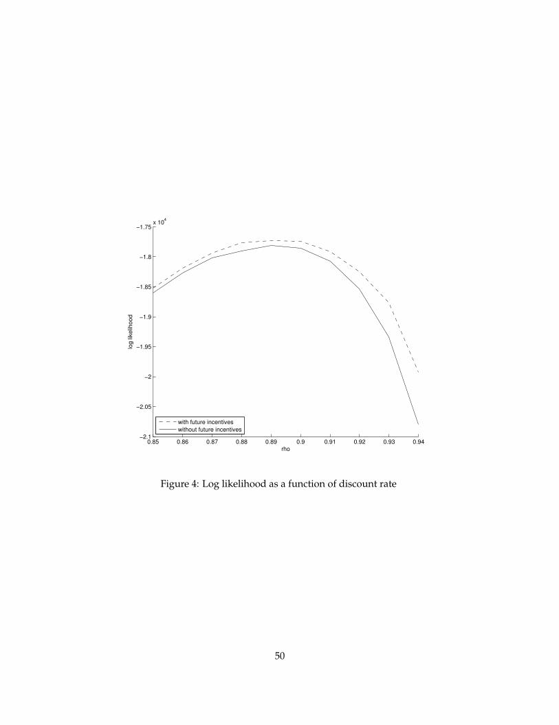
0.85 0.86 0.87 0.88 0.89 0.9 0.91 0.92 0.93 0.94−2.1

−2.05

−2

−1.95

−1.9

−1.85

−1.8

−1.75x 10

4

rho

log lik

elih

oo

d

with future incentives

without future incentives

Figure 4: Log likelihood as a function of discount rate

50

2002 2004 2006 2008 2010 2012 2014 2016 2018 2020 20220

0.1

0.2

0.3

0.4

0.5

0.6

0.7

0.8

0.9

1

year

fraction

of firm

s g

ree

n

all

reg

grants

fee

none

Figure 5: The fraction of cleaners using green equipment with different policy tools (no demon-strations)

51

2002 2004 2006 2008 2010 2012 2014 2016 2018 2020 2022−0.5

0

0.5

1

year

% c

hang

e d

ue

to d

em

onstr

atio

n s

ites

perc

CA HC

CA GE

CA wet

CA CO2

Figure 6: The relative difference in the number of green cleaners with and without demonstrationsites.

52

2002 2004 2006 2008 2010 2012 2014 2016 2018 2020 20220

0.2

0.4

0.6

0.8

1

1.2

1.4

1.6

1.8

2

year

num

ber

of

firm

s

all

reg

grants

fee

Figure 7: The number of cleaners relative to no policy

53

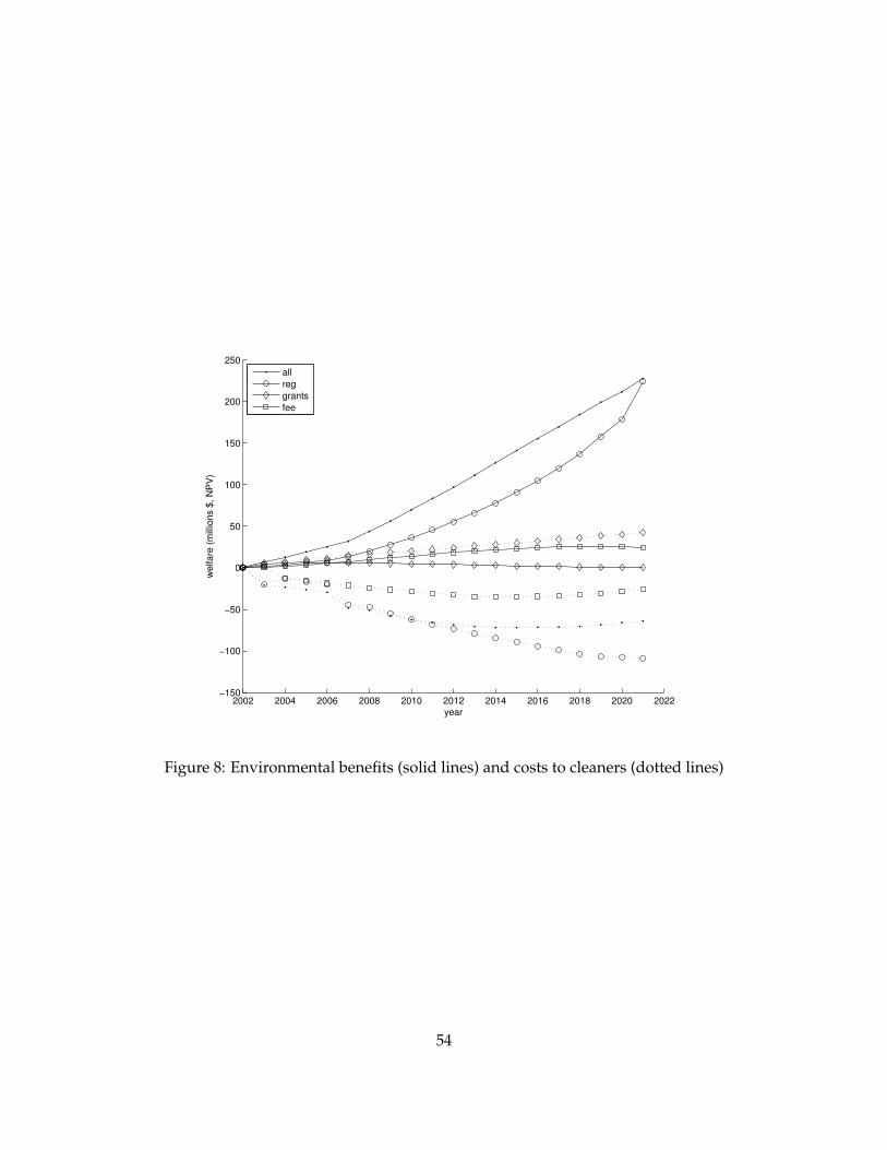
2002 2004 2006 2008 2010 2012 2014 2016 2018 2020 2022−150

−100

−50

0

50

100

150

200

250

year

we

lfare

(m

illio

ns $

, N

PV

)

all

reg

grants

fee

Figure 8: Environmental benefits (solid lines) and costs to cleaners (dotted lines)

54

2002 2004 2006 2008 2010 2012 2014 2016 2018 2020 2022−10

−5

0

5

10

15

20

year

co

st o

f g

ran

ts (

mill

ions $

, N

PV

)

all

grants

fee

Figure 9: Tax revenue/costs for fees and grants

55

2002 2004 2006 2008 2010 2012 2014 2016 2018 2020 2022−50

0

50

100

150

200

year

we

lfare

(m

illio

ns $

, N

PV

)

all

reg

grants

fee

Figure 10: Net Welfare

56