31

161

Dr. Yoram Tal

� � � � � � � � � �

Gray scale

162

Dr. Yoram Tal

g2 = ordfilt2 ( g1,n,se) ;

� � � � � � � � � � � � � � � � � � �

Order fi lter: replace the central pixel by the n-th element of the sorted image neighborhood pixel list.

0 0 1 1 0 00 1 1 1 1 01 1 1 1 1 11 1 1 1 1 10 1 1 1 1 00 0 1 1 0 0

se

M = sum(se(:) > 0); % number of positive elements

n = 1: minimum (erosion)

n = M: maximum (dilation)

n = M/2: median

Gray Scale Morphology

Replace dilation/erosion by maximum/minimum

dilation

( )( , ) max{ ( , ) ( , )

|( ),( ) ,( , ) }f b

f b s t f s x t y b x ys x t y D x y D

⊕ = − − +− − ∈ ∈

domain of

domain of , are functions not sets

f

b

D fD bf b

=

=

One Dimension

( )( ) max{ ( ) ( )

|( ) , }f b

f b s f s x b xs x D x D

⊕ = − +− ∈ ∈

Note, we shift f rather than the structuring element. Usually, bD is smaller than fD (figure 9:36)

smoothing is accomplished by opening followed by closing

(figure 9:38)

gradient: ( ) ( )g f b f b= ⊕ − (figure 9:39)

top-hat: ( )h f f b= − (figure 9:40)

Gray-value morphological processing

The techniques of morphological filtering can be extended to gray-levelimages. To simplify matters we will restrict our presentation to structuringelements, B, that comprise a finite number of pixels and are convex andbounded. Now, however, the structuring element has gray values associatedwith every coordinate position as does the image A.

* Gray-level dilation, DG(*), is given by:

Dilation -

For a given output coordinate [m,n], the structuring element is summed with ashifted version of the image and the maximum encountered over all shiftswithin the J x K domain of B is used as the result. Should the shifting requirevalues of the image A that are outside the M x N domain of A, then a decisionmust be made as to which model for image extension, as described in Section9.3.2, should be used.

* Gray-level erosion, EG(*), is given by:

Erosion -

The duality between gray-level erosion and gray-level dilation--the gray-levelcounterpart of eq. --is somewhat more complex than in the binary case:

Duality -

where " " means that a[j,k] -> -a[-j,-k].

The definitions of higher order operations such as gray-level opening andgray-level closing are:

Opening -Closing -

The important properties that were discussed earlier such as idempotence,translation invariance, increasing in A, and so forth are also applicable to graylevel morphological processing. The details can be found in Giardina andDougherty .

In many situations the seeming complexity of gray level morphologicalprocessing is significantly reduced through the use of symmetric structuringelements where b[j,k] = b[-j,-k]. The most common of these is based on theuse of B = constant = 0. For this important case and using again the domain[j,k] B, the definitions above reduce to:

Dilation -

Erosion -

Opening -

Closing -

The remarkable conclusion is that the maximum filter and the minimum filter,introduced in Section 9.4.2, are gray-level dilation and gray-level erosion forthe specific structuring element given by the shape of the filter window withthe gray value "0" inside the window. Examples of these operations on asimple one-dimensional signal are shown in Figure 45.

a) Effect of 15 x 1 dilation and erosion b) Effect of 15 x 1 opening and closing

Figure 45: Morphological filtering of gray-level data.

For a rectangular window, J x K, the two-dimensional maximum or minimumfilter is separable into two, one-dimensional windows. Further, a one-dimensional maximum or minimum filter can be written in incremental form.(See Section 9.3.2.) This means that gray-level dilations and erosions have acomputational complexity per pixel that is O(constant), that is, independent ofJ and K. (See also Table 13.)

The operations defined above can be used to produce morphologicalalgorithms for smoothing, gradient determination and a version of theLaplacian. All are constructed from the primitives for gray-level dilation andgray-level erosion and in all cases the maximum and minimum filters aretaken over the domain .

Morphological smoothing

This algorithm is based on the observation that a gray-level openingsmoothes a gray-value image from above the brightness surface given by thefunction a[m,n] and the gray-level closing smoothes from below. We use astructuring element B based on eqs. and .

Note that we have suppressed the notation for the structuring element Bunder the max and min operations to keep the notation simple.

Morphological gradient

For linear filters the gradient filter yields a vector representation (eq. (103))with a magnitude (eq. (104)) and direction (eq. (105)). The version presentedhere generates a morphological estimate of the gradient magnitude:

Morphological Laplacian

The morphologically-based Laplacian filter is defined by:

Summary of morphological filters

The effect of these filters is illustrated in Figure 46. All images were processedwith a 3 x 3 structuring element as described in eqs. through . Figure 46e wascontrast stretched for display purposes using eq. (78) and the parameters 1%and 99%. Figures 46c,d,e should be compared to Figures 30, 32, and 33.

a) Dilation b) Erosion c) Smoothing

d) Gradient e) Laplacian

Figure 46: Examples of gray-level morphological filters.

34

167

Dr. Yoram Tal

Â Ã Ä Å Æ Ç Ä È É Ê Ë Ì Í Î Ë Ï Ë Ð Ñ Ò Ó Ô Õ Ö × Ø Ù Ú ÕOr i gi nal si gnal

L i ne ar f i l ter i ng (gaussi an)

168

Dr. Yoram TalÛ Ü Ý Þ ß à Ý á â ã ä å æ ç ä è ä é ê ë ì í î ï ð ñ ò ó î ô õ öOriginal signal

Window size(Structuring element)

Erosion

Dilation

35

169

Dr. Yoram Tal

÷ ø ù ú û ü ù ý þ ÿ � ø � � � ý � � ú � � � þ � ù � � ý þ �Original signal

Openning = erosion + dilation

Closing = dilation + erosion

170

Dr. Yoram Tal

Grayscale Morphology

Black 255White 0

Erosion

Dilation

33

165

Dr. Yoram Tal

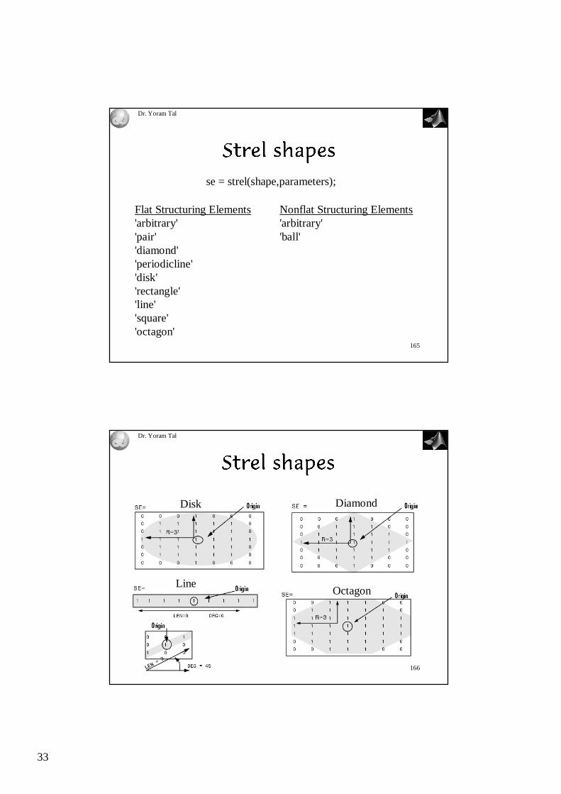
¹ º » ¼ ½ ¾ ¿ À Á ¼ ¾se = strel(shape,parameters);

Flat Structuring Elements'arbitrary''pair''diamond''periodicline''disk''rectangle''line''square''octagon'

Nonflat Structuring Elements'arbitrary''ball'

166

Dr. Yoram Tal ¹ º » ¼ ½ ¾ ¿ À Á ¼ ¾Disk Diamond

LineOctagon

25

149

Dr. Yoram Tal É Ê Ë Ì Í Î Ï Ë Ð Ñ Ò Ó Ô Õconndef Default connectivity arrayimbothat Perform bottom-hat filteringimclearborder Suppress li ght structures connected to image borderimclose Close imageimdilate Dilate imageimerode Erode imageimextendedmax Extended-maximatransformimextendedmin Extended-minima transformimfill Fill image regions imhmax H-maximatransformimhmin H-minima transformimimposemin Impose minimaimopen Open imageimreconstruct Perform morphological reconstruction imregionalmax Regional maximaof imageimregionalmin Regional minima of imageimtophat Perform tophat filteringwatershed Find image watershed regions

150

Dr. Yoram Tal Ö × Ø Ù Ó Ú Û Ù Ü Ù Ý Õ Þ ß à

bw2 = dilate(bw1,se); % se general structuring elementbw2 = erode(bw1,se);bw2 = bwmorph(bw1,opt,N) % opt defines a 3x3 se

' bothat' Subtra ct the in put imag e from i t s closin g ' bridge' Bridge previous l y uncon nected p i xels ' clean' Remove isolated pixels ' close' Perfor m binary closure ' diag' Diagon al fill t o elimin ate 8- connecti vity ' dilate' Perfor m dilatio n ' erode' Perfor m erosion ' f ill' Fill i solated i nterior pixels ' hbreak' Remove H- connecte d pixels ' majority ' ' open' Perfor m binary opening ' r emove' findon l y bounda r y pixel s ' shrink' ' skel' skelet onization ' spur' Remove end poin t s of li nes ' t hicken' ' t hin' ' t ophat' Subtra ct the op ening fr om the i nput imag e

32

163

Dr. Yoram Tal� � � � �   � ¡ ¢ £ ¤ � ¥ ¦ ¤ ¡ ¤ § �¨ � © ª « ¬ ª   ­ © ¤ ª �

imbothat Perform bottom-hat filteringimclose Close imageimdilate Dilate imageimerode Erode imageimfill Fill image regions imopen Open imageimreconstruct Perform morphological reconstruction imtophat Perform tophat filteringwatershed Find image watershed regionsstrel structuring element

164

Dr. Yoram Tal® ¯ ° ± ² ³ ´ ¯ ° µ ¶ ¯ µ ° ± ± ² ± · ± ¸ ¯Creation and Manipulation

getheight Get the height of a structuring elementgetneighbors Get structuring element neighbor locations and heights

(coordinate li st)getnhood Get structuring element neighborhood (matrix)getsequence Extract sequence of decomposed structuring elementsisflat Return true for flat structuring elementreflect Reflect structuring elementstrel Create morphological structuring elementTranslate Translate structuring element

36

171

Dr. Yoram Tal

Grayscale Opening

� � � � � � � � �� � � � � �

172

Dr. Yoram Tal

Grayscale Opening

� � � � � � � � �� � � � � �

37

173

Dr. Yoram Tal

Grayscale Opening

� � � � � � � � �� � � � � �

174

Dr. Yoram Tal

� � � � � � � � � � � ! " � � # $ %

Letter

x = ordfilt2 (Letter,49,ones(7) , s ymm ) ; % di la t i ony = ordfilt2 ( x,1,ones(7),'symm'); % er os i on

y

Step 1: background reconstruction via closing operation

38

175

Dr. Yoram Tal

& ' ( ) * + ( , - - . ( / 0 , - 1 2 3Step 2: background subtraction Step 3: Thresholding

Top hat (bottom hat) operation:

Z = Letter y; Z > Threshold

176

Dr. Yoram Tal4 5 6 7 8 9 6 : ; ; < 6 = > : ; ? @ A

Example taken from the demo files of the SDC Morphology toolbox v0.13

39

177

Dr. Yoram Tal B C D C E F B C F C E F G H IThe input image is a gray-scale image of a microelectronic circuit. The relevant objects in this image are vertical metal stripes. These stripes have some irregularities that should be detected.

Source gradient projection

178

Dr. Yoram Tal J K L M N O P

Closing of the image by a vertical line of length 25 pixels.

Close surf

40

179

Dr. Yoram Tal Q R S T U V W X S Y Z [ \ ]Subtraction of the closing from the original is called closing top-hat. It shows the discrepancies of the image where the structuring element cannot fit the surface. In this case, it highlights vertical depression with length longer than 25 pixels.

Close surf

180

Dr. Yoram Tal^ _ ` a b _ c d e f g h i j k l m n o n p

41

181

Dr. Yoram Tal q r s t u v

182

Dr. Yoram Tal w x y z x { | } | ~ � {

The idea of segmentation has its roots in work by Gestalt psychologist (e.g. Kohler) who studied the preferences exhibitedby human beings in grouping or organizing sets of shapes arranged in the visual field. (Ballard & Brown)

Segmentation is the first essential and important step of low-level vision (Marr, Rosenfeld, Hall , Gonzalez, in Pal & Pal).

Morphological Image Processing Lecture 22 (p. 19)

9.6 Extensions to grey-scale images

f(x, y): Input imageb(x, y): Structuring element image

9.6.1 Dilation

Grey-scale dilation of f by b, is defined as

(f ⊕ b)(s, t) = max {f(s− x, t− y) + b(x, y)|(s− x), (t− y) ∈ Df ; (x, y) ∈ Db} ,

where Df and Db are the domains of f and b, respectively

Morphological Image Processing Lecture 22 (p. 20)

Simple 1D example. For functions of one variable:

(f ⊕ b)(s) = max {f(s− x) + b(x)|(s− x) ∈ Df ; x ∈ Db}

General effect of dilation of a grey-scale image:

(1) If all values of b(x, y) are positive; output image brighter

(2) Dark details are reduced or eliminated, depending on size

Morphological Image Processing Lecture 22 (p. 21)

9.6.2 Erosion

Grey-scale erosion of f by b, is defined as

(f ª b)(s, t) = max {f(s + x, t + y)− b(x, y)|(s + x), (t + y) ∈ Df ; (x, y) ∈ Db} ,

where Df and Db are the domains of f and b, respectively

Simple 1D example. For functions of one variable:

(f ª b)(s) = max {f(s + x)− b(x)|(s + x) ∈ Df ; x ∈ Db}

Morphological Image Processing Lecture 22 (p. 22)

General effect of erosion of a grey-scale image:

(1) If all values of b(x, y) are positive ; output image darker

(2) Bright details are reduced or eliminated, depending on size

Example 9.9: Dilation and erosion on grey-scale image

f(x, y): 512 x 512b(x, y): “flat top”, unit height, size of 5 x 5

Morphological Image Processing Lecture 22 (p. 23)

9.6.3 Opening and closing

The opening of image f by b, is defined as

f ◦ b = (f ª b)⊕ b

The closing of image f by b, is defined as

f ◦ b = (f ⊕ b)ª b

Explanation using “rolling ball”:

Morphological Image Processing Lecture 22 (p. 24)

Opening and closing of “horse image”:

9.6.4 Some applications of grey-scale morphology

Morphological smoothing

Opening followed by closing; remove or attenuate bright anddark artifacts or noise

Morphological Image Processing Lecture 22 (p. 25)

Morphological gradient

Definition: g = (f ⊕ b)− (f ª b)

Top-hat transformation

Definition: h = f − (f ◦ b)