Bachelor Thesis Physics and Astronomy

Gravitational wave emissionsfrom

Low Mass X-ray Binaries

Author:Manuel Oppenoorth5789389

Supervisor:Dr. Brynmor Haskell

Second corrector:Dr. Anna Watts

Size 12 EC, research conducted betweenMay 1, 2011 and December 21, 2011

21st December 2011

Astronomical Institute Anton PannekoekFaculteit der Natuurwetenschappen, Wiskunde en Informatica

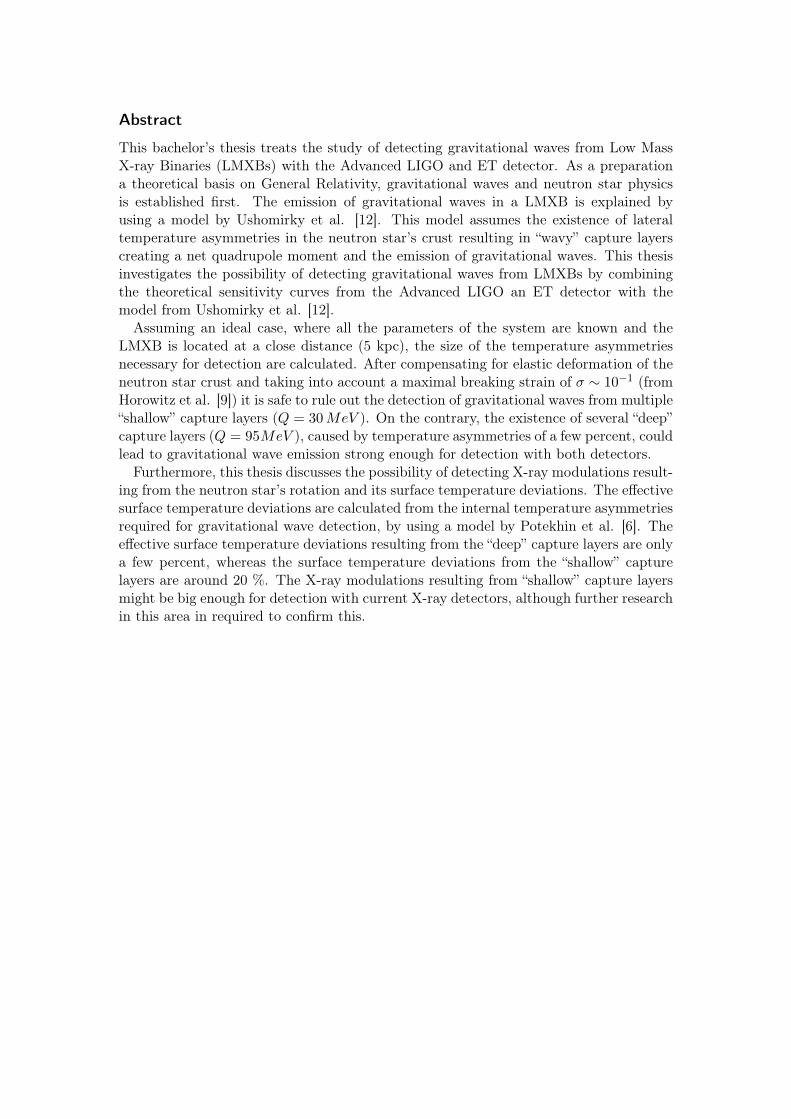
Abstract

This bachelor’s thesis treats the study of detecting gravitational waves from Low MassX-ray Binaries (LMXBs) with the Advanced LIGO and ET detector. As a preparationa theoretical basis on General Relativity, gravitational waves and neutron star physicsis established first. The emission of gravitational waves in a LMXB is explained byusing a model by Ushomirky et al. [12]. This model assumes the existence of lateraltemperature asymmetries in the neutron star’s crust resulting in “wavy” capture layerscreating a net quadrupole moment and the emission of gravitational waves. This thesisinvestigates the possibility of detecting gravitational waves from LMXBs by combiningthe theoretical sensitivity curves from the Advanced LIGO an ET detector with themodel from Ushomirky et al. [12].

Assuming an ideal case, where all the parameters of the system are known and theLMXB is located at a close distance (5 kpc), the size of the temperature asymmetriesnecessary for detection are calculated. After compensating for elastic deformation of theneutron star crust and taking into account a maximal breaking strain of σ ∼ 10−1 (fromHorowitz et al. [9]) it is safe to rule out the detection of gravitational waves from multiple“shallow” capture layers (Q = 30MeV ). On the contrary, the existence of several “deep”capture layers (Q = 95MeV ), caused by temperature asymmetries of a few percent, couldlead to gravitational wave emission strong enough for detection with both detectors.

Furthermore, this thesis discusses the possibility of detecting X-ray modulations result-ing from the neutron star’s rotation and its surface temperature deviations. The effectivesurface temperature deviations are calculated from the internal temperature asymmetriesrequired for gravitational wave detection, by using a model by Potekhin et al. [6]. Theeffective surface temperature deviations resulting from the “deep” capture layers are onlya few percent, whereas the surface temperature deviations from the “shallow” capturelayers are around 20 %. The X-ray modulations resulting from “shallow” capture layersmight be big enough for detection with current X-ray detectors, although further researchin this area in required to confirm this.

Populair wetenschappelijke samenvatting:

Emissie van gravitatiegolven door neutronensterren in dubbelstersystemen

In dit bachelorproject word de emissie van gravitatiegolven door neutronen sterren indubbelstersystemen beschreven en wordt onderzocht of deze gravitatiegolven waar tenemen zijn met de Advanced LIGO en ET detector. De Advanced LIGO detector is opdit moment onder constructie in de VS en moet rond 2016 in werking treden. De ETdetector is nog in de ontwerpfase en staat gepland om over 10 jaar af te zijn.

Om te begrijpen wat gravitatiegolven zijn moeten we eerst terug in de tijd naar hetjaar 1916. In dit jaar publiceerde Albert Einstein zijn beroemde algemene relativiteitstheorie (ART), die ons begrip van zwaartekracht, ruimte én tijd volledig zou veranderen.Volgens ART vormen ruimte en tijd samen een geheel, namelijk de vierdimensionaleruimtetijd. Drie ruimtelijke dimensies (lengte, breedte en hoogte) en één tijd dimensie.ART beschrijft ook de zwaartekracht, die volgens deze theorie niets meer of minder isdan de vervorming of kromming van de ruimtetijd.

Een voorspelling van ART is het bestaan van gravitatiegolven. Net als (water)golvenzich over het oppervlak van een vijver voortplanten, zo planten gravitatiegolven zichvoort door de ruimtetijd. Hierbij vervormen de gravitatiegolven tijdelijk deze ruimtetijd.

Gravitatiegolf detectoren maken gebruik van deze vervorming om gravitatiegolven tedetecteren. De detectoren bestaan uit twee loodrecht aan elkaar geplaatste buizen (vanwel 20 kilometer lang) waar lasers door gestuurd worden. Op het moment dat er eengravitatiegolf langs komt wordt één van de twee buizen een klein beetje korter terwijlde andere langer wordt. Dit lengte verschil kan gemeten worden door het verschil in deaankomsttijd van het licht van de lasers te meten. Omdat gravitatiegolven zo verschrikke-lijk zwak zijn hebben we deze enorme detectoren met hele precieze meetinstrumentennodig om ze te kunnen meten.

Gravitatiegolven ontstaan onder andere in ronddraaiende neutronensterren waarbij demassa niet gelijkmatig is verdeeld. Neutronensterren ontstaan als een gewone ster, meteen massa van 10-15 keer de massa van onze zon, aan het einde van zijn leven komten ontploft in een supernovae explosie. Het restant van deze explosie is een neutronen-ster. Neutronensterren zijn heel klein (straal van ongeveer 10 km), hebben een enormedichtheid (1 theelepel “neutronenster” heeft een massa van 900 keer de piramide vanGizeh) en grote rotatiesnelheden (rotatieperiodes tussen de 1.4 milliseconden en 30 sec-onden).

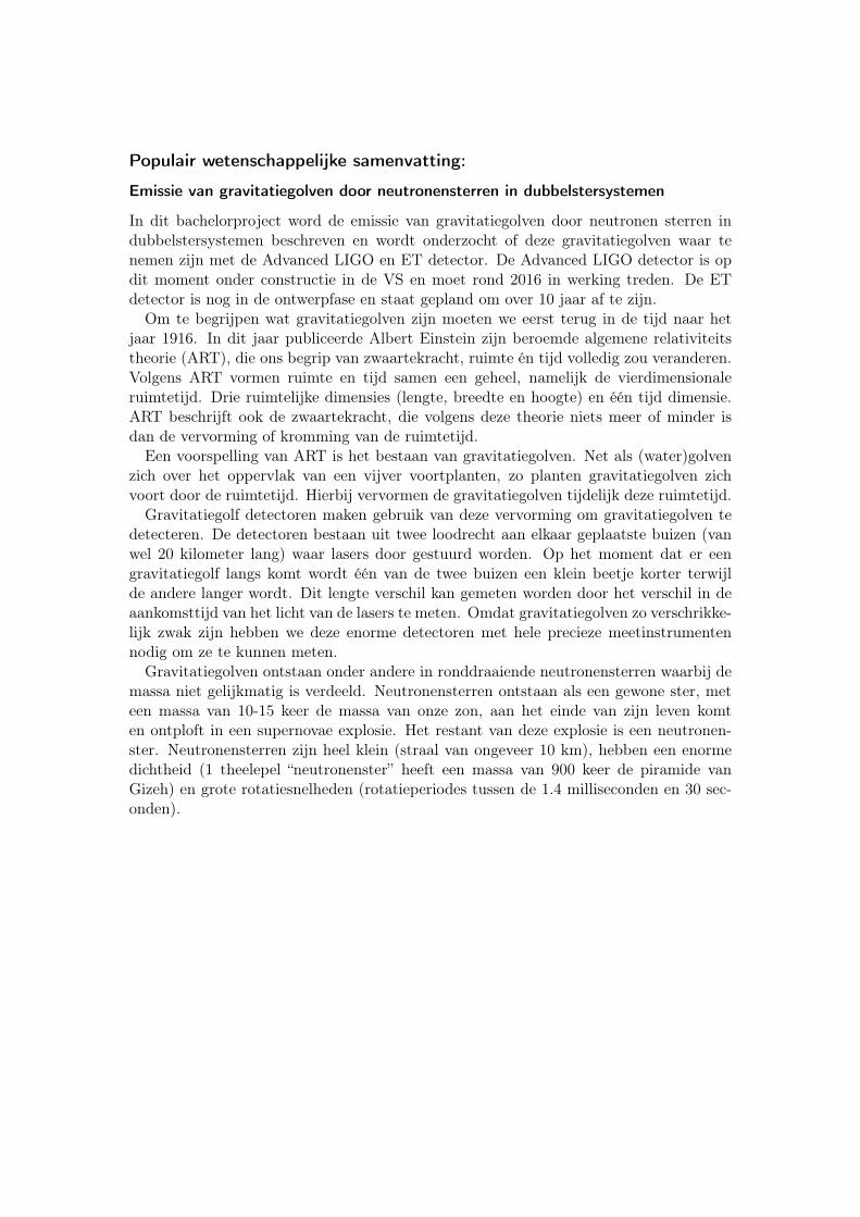
Figure 1: Dubbelstersysteem met rechts de neutronenster, die materie van de begelei-dende ster (links) naar zich toe trekt en daardoor Röntgen straling uitzendt.Bron: [8].

Soms komen neutronensterren voor in een dubbelstersysteem zoal in figuur 1. Door deenorme zwaartekracht van de neutronenster trekt deze materie van de andere ster naarzich toe, waarbij de neutronenster erg heet wordt en Röntgenstraling gaat uitzenden (dewitte stralen in de figuur). Als dit proces niet symmetrisch verloopt (door bijvoorbeeldhet sterke magneetveld van de neutronenster) dan ontstaan er temperatuur verschillenin de korst (de buitenste lagen) van de neutronen ster. Deze temperatuurverschillenleiden tot dichtheidheidsverschillen en in combinatie met de rotatie van de neutronensterresulteert dit in de emissie van gravitatiegolven.

In dit bacheloronderzoek is o.a. gekeken naar hoe groot de asymmetrische temperatuurverschillen moeten zijn, om gravitatiegolven te krijgen die gedetecteerd kunnen wordenmet de Advanced LIGO of ET detector. Uit het onderzoek valt te concluderen datasymmetrische temperatuurverschillen in de ondiepe lagen van de korst onvoldoendezijn voor detectie. Daarentegen zijn temperatuurverschillen van een paar procent in dediepere lagen van de korst waarschijnlijk voldoende om gravitatiegolven te detecteren metzowel de Advanced LIGO als de ET detector. Onderzoek van Ushomirsky en anderen[12] heeft uitgewezen dat, in dubbelstersystemen zoals deze, asymmetrische temperatuurverschillen van dit formaat kunnen ontstaan.

Als er in de toekomst daadwerkelijk gravitatiegolven van dit soort systemen wordenwaargenomen, is dat een bevestiging van Einstein’s ART en kan dit tot nieuwe inzichtenleiden in de structuur van neutronensterren.

Contents

1 Introduction 7

2 General Relativity 8

2.1 Equations of General Relativity . . . . . . . . . . . . . . . . . . . . . . . . 82.2 Linearized theory of gravity . . . . . . . . . . . . . . . . . . . . . . . . . . 9

3 Gravitational waves 10

3.1 Gauge invariance . . . . . . . . . . . . . . . . . . . . . . . . . . . . . . . . 113.2 Propagation of gravitational waves . . . . . . . . . . . . . . . . . . . . . . 133.3 Polarization of gravitational waves . . . . . . . . . . . . . . . . . . . . . . 143.4 Generation of gravitational waves . . . . . . . . . . . . . . . . . . . . . . . 153.5 Detection of gravitational waves . . . . . . . . . . . . . . . . . . . . . . . . 17

3.5.1 Detector types . . . . . . . . . . . . . . . . . . . . . . . . . . . . . 193.5.2 Existing and future gravitational wave detecters . . . . . . . . . . . 21

4 Neutron stars 24

4.1 Neutron star structure . . . . . . . . . . . . . . . . . . . . . . . . . . . . . 254.2 Neutron star types . . . . . . . . . . . . . . . . . . . . . . . . . . . . . . . 274.3 Neutron stars in binary systems . . . . . . . . . . . . . . . . . . . . . . . . 274.4 Gravitational wave emission . . . . . . . . . . . . . . . . . . . . . . . . . . 29

5 Gravitational wave emission in LMXBs 30

5.1 Quadrupole emergence . . . . . . . . . . . . . . . . . . . . . . . . . . . . . 305.1.1 Composition and temperature asymmetries through accretion . . . 305.1.2 Resulting quadrupole moment . . . . . . . . . . . . . . . . . . . . . 31

5.2 Sensitivity measurements . . . . . . . . . . . . . . . . . . . . . . . . . . . 325.3 Surface temperatures and X-ray modulations . . . . . . . . . . . . . . . . 345.4 Discussion . . . . . . . . . . . . . . . . . . . . . . . . . . . . . . . . . . . . 37

6 Conclusion & Outlook 40

7 Acknowledgements 41

8 Appendices 42

8.1 Mathematics and notations for General Relativity . . . . . . . . . . . . . . 428.1.1 Einstein summation . . . . . . . . . . . . . . . . . . . . . . . . . . 428.1.2 Tensors . . . . . . . . . . . . . . . . . . . . . . . . . . . . . . . . . 438.1.3 Metric tensor . . . . . . . . . . . . . . . . . . . . . . . . . . . . . . 438.1.4 Tensor operations . . . . . . . . . . . . . . . . . . . . . . . . . . . . 44

8.2 Details on computations, simulations and graphics . . . . . . . . . . . . . 45

References 48

6

1 Introduction

The subject of this thesis is the study of Low Mass X-ray Binaries (LMXBs) and theirgravitational wave emission during accretion. In particular, we discuss the circumstancesrequired for detection with the Advanced LIGO and ET detector. These two gravitationalwave detectors are currently being build, and planned operational between 5 and 10years respectively. The detection of these gravitational waves could explain why LMXBsreach a certain boundary in the rotation speed and might lead to new insights in thecomposition and structure of the neutron star’s internal.

In this thesis we used the sensitivity curves of the Advanced LIGO and ET detectorand a model by Ushomirsky et al. [12], to estimate the possibility of detecting gravita-tional waves from LMXBs with these detectors. The model from Ushomirsky et al. [12]describes the emission of gravitational waves resulting from temperature asymmetries inthe interior of the neutron star.

In the research done for this thesis, we use this model to calculate the size of theseinternal temperature asymmetries required for detection. In addition we looked at theresulting surface temperature deviations and their possibility of detection with X-raytelescopes, using a model by Potekhin et al. [6].

The results and conclusions of the research done, can be found in the second part of thisthesis, i.e. chapters 5 and 6. The first part of the thesis (chapters 2-4) serves as introduc-tional material, it consists of necessary background information for the understanding ofthe second part. The rest of the thesis is made up of: 7 Acknowledgements, chapter 8Appendices and a list of References.

7

2 General Relativity

In order to study gravitational waves we need to look at the framework in which gravita-tional waves are expressed. This is the theory of General Relativity by Albert Einstein.General Relativity is a concise and complete theory which is able to explain all gravita-tional interactions in the universe. If we want to discuss General Relativity in more detailwe need to understand the language in which it’s written, the language of mathematics.Appendix 8.1 describes some of the new notations necessary for the understanding ofGeneral Relativity.

Einsteins theory of General Relativity originated from the thought that: “ the pro-portionality between the inertial and the gravitational mass of a body is an exact law ofnature that must be expressed as a foundation principle of theoretical physics.” This isthe so called Equivalence hypothesis, which in other words states that it’s impossible totell the difference between an object at rest in a gravitational field or an accelerating ob-ject in free space, where the acceleration is generated by a force equal to the gravitationalfield. This resulted in a description of gravity as a geometric property of spacetime. Inshort: “Geometry tells matter how to move, and matter tells geometry how to curve.”

-John Archibald Wheeler-

2.1 Equations of General Relativity

The relation between matter and geometry is specified by the Einstein field equations.Which are a set of nonlinear differential equations.

Gαβ =8πG

c4Tαβ (1)

with Tαβ the stress-energy tensor, Gαβ the Einstein tensor, G the gravitational constantand c the speed of light. For the remainder of this thesis c and G are set equal to 1. Thischanges eqn. 11 into

Gαβ = 8πTαβ . (2)

“The field equation shows how the stress-energy of matter generates an average curvatureGαβ in its neighborhood. Simultaneously, the field equation is a propagation equationfor the remaining, anisotropic part of the curvature: it governs the external spacetimecurvature of a static source; it governs the generation of gravitational waves by stress-energy in motion; and it governs the propagation of those waves through the universe.The field equation even contains within itself the equations of motion for the matterwhose stress-energy generates the curvature.”[10] The Stress-energy tensor Tαβ is a toolto detemine how much mass-energy there is in a unit volume, it’s linear and symmetric(Tαβ = T

βα).The Einstein tensor Gαβ is always generated directly by the local distribution of matter,

i.e. it’s only constructed from the Riemann curvature tensor (Rγαγβ) and the metric

tensor (gαβ). The metric tensor is an object which describes us how spacetime is curved.By definition; The distance between two points in spacetime is the infinitesimal element

8

ds with length,ds ≡

�gαβdx

αdxβ . (3)

for more on the metric tensor see the appendix 8.1.3.

Gαβ = Rαβ − 1

2Rgαβ (4)

With Rαβ = Rγαγβ the Ricci tensor and R i’ts trace or the Ricci scalar. The Riemann

curvature tensor given by:

Rρσαβ = ∂αΓ

ρβσ − ∂βΓ

ρασ + Γρ

αγΓγβσ − Γρ

βγΓγασ (5)

with Γραβ the so called Christoffel symbols,

Γραβ =

1

2gργ(∂αgβγ + ∂βgγα − ∂γgαβ) (6)

The Einstein tensor Gαβ is a symmetric tensor that’s linear in Riemann and vanisheswhen spacetime is flat. As stated in [10]; ∇ · G ≡ 0 for any smooth Riemmannianspacetime. This is called the “automatic conservation of the source”, which results inthe fact that there are only six field equations 2, instead of ten. “The four conservationlaws G

αβ ;α ≡ 0 do not constrain in any way the evolution of the geometry”, [10]. TheRiemann tensor it self is symmetric under pair exchange: Rαβγδ = Rγδαβ .

2.2 Linearized theory of gravity

In situations where only weak gravitational fields are present one can use the linearizedtheory of gravity. In this theory the metric gαβ is given by,

gαβ = ηαβ + hαβ , | hαβ |� 1 (7)

with ηαβ the minkowski metric for flat space time (see appendix 8.1.3), and hαβ a verysmall pertubation (which is also symmetric, hαβ = hβα). In these situations the fieldequations 2 can be expanded in powers of hαβ . Since | hαβ |� 1 (which also applies toall derivatives of hαβ) one can omit all second and higher order terms, leaving the fieldeqations linear in hαβ . In linearized theory it is conventional, that if one expands inpowers of hαβ , one raises or lowers indices by using η

αβ and ηαβ and not gαβ and gαβ .

From equation 43 we can find that the inverse metric of gαβ is given by,

gαβ = η

αβ − hαβ

.

9

3 Gravitational waves

Gravitational waves are a direct prediction of Einsteins theory of General Relativity.Only a few assumptions are necessary in order to let them emerge directly from the fieldequations 2. Let’s consider a (small) gravitational wave travelling through empty spacei.e. space time is flat and only the wave creates a small pertubation in the metric. Underthese conditions it’s possible to use the linearized theory of gravity as described in section2.2.

If we plug the metric 7 into the Christoffel symbols 6 we end up with,

Γραβ =

1

2ηργ(hβγ,α + hαγ,β − hαβ,γ), (8)

using the fact that ηαβ,γ = 0, ηαγ,β = 0 and ηβγ,α = 0 and that hαβ is symmetric. TheRiemann curvature tensor is then found by inserting equation 8 in equation 5, keepingonly linear terms in hαβ results in,

Rρσαβ =

1

2

�(hρβ,ασ + h

ρσ,αβ − h

ρσβ,α)− (hρσ,αβ + h

ρα,σβ − h

ρασ,β)

�=

1

2

�hρβ,ασ − h

ρσβ,α − h

ρα,σβ + h

ρασ,β

�.

The Ricci tensor is then given by,

Rσβ =1

2

�hρβ,ρσ − h

ρσβ,ρ − h

ρρ,σβ + h

ρρσ,β

�=

1

2

�hρβ,ρσ + h

ρρσ,β −�hσβ − h,σβ

�(9)

with � = ∂ρ∂ρ and h

ρρ = h.

The Ricci scalar is then given by,

R = ησβRσβ = h

ρ ββ,ρ −�h. (10)

Using equations 9 and 10 the equations of motion for the gravitational pertubationcan be obtained by equation 4,

hρβ,ρα + h

ρρα,β −�hαβ − h,αβ − (hρ β

β,ρ −�h)gαβ = 16πTαβ (11)

This can be rewritten in the following form,

−�hαβ + (hρβ,ρα + hρ

ρα,β − h,αβ) = 16πTαβ + gαβ(hρ ββ,ρ −�h). (12)

In order to write equation 12 even shorter we first have to take a look at the trace ofTαβ using the fact that 16πT = 16πgαβTαβ and equation 11.

16πT = gαβ

�hρβ,ρα + h

ρρα,β −�hαβ − h,αβ − (hρ β

β,ρ −�h)gαβ�

16πT = ηαβ(hρβ,ρα + h

ρρα,β −�hαβ − h,αβ)− g

αβgαβ(h

ρ ββ,ρ −�h)

16πT = hρ ββ,ρ + h

β ρρ,β −�h−�h− 4(hρ β

β,ρ −�h) = −2(hρ ββ,ρ −�h),

10

resulting in:−8πgαβT = gαβ(h

ρ ββ,ρ −�h). (13)

Therefore equation 12 can be written as,

−�hαβ + (hρβ,ρα + hρ

ρα,β − h,αβ) = 16π(Tαβ − 1

2gαβT ) (14)

Although it’s far from trivial to solve the above equations in general, it is possible insome occasions, as can be seen in section 3.2 .

3.1 Gauge invariance

As shown in section 2.1 there are only six equations in 1 that constrain the evolutionof geometry in contrast with the ten equations of the metric gαβ . The remaining fourequations of gαβ allow us to adjust the coordinate system, without affecting any observ-able. The gauge of choice is the tensor equivalent of the Lorentz gauge, with the gaugecondition,

hαβ ,α =

1

2hρρ,β (15)

The equations of motion 14 can now be rewritten as,

−�hαβ + (1

2hρρ,βα +

1

2hρρ,αβ − h,αβ) = −�hαβ + (h,αβ − h,αβ) = (16)

−�hαβ = 16π(Tαβ − 1

2gαβT ) (17)

Let us definehαβ ≡ hαβ − 1

2ηαβh (18)

and let us rewrite the gauge condition 15,

hαβ ,α − 1

2hρρ,β = 0

hρα

,α − 1

2ηραh,α = 0

which is the same as,hρα

,α = 0. (19)

11

Using this new notation we can rewrite the equations of motion 17, once more usingequation 18,

�hαβ = �hαβ − 1

2ηαβ�h

= −16πTαβ + 8gαβT − 1

2ηαβ�h

using equation 13,

= −16πTαβ − ηαβ(hρ ββ,ρ −�h)− 1

2ηαβ�h

= −16πTαβ − ηαβhρ ββ,ρ +

1

2ηαβ�h

= −16πTαβ − ηαβ∂β(hρβ,ρ −

1

2h,β)

using the gauge condition 15,

= −16πTαβ − ηαβ∂β(hρβ,ρ − h

ρβ,ρ)

Resulting in the final form:�hαβ = −16πTαβ (20)

We succeeded to find a formalism in which the equations of motion are of a compactform, moreover they are also of great physical importance. The equations of motion of asmall gravitational pertubation are an (inhomogeneous) wave equation for hαβ .

12

3.2 Propagation of gravitational waves

In the previous section we described the equations of motion for a small gravitationalpertubation in a flat background spacetime and we introduced the gauge conditions inorder to obtain a wave equation, see equation 20. Let’s solve these equations in vacuumi.e. Tαβ = 0, this reduces the equations to the familiar form,

�hαβ = 0 (21)

the homogeneous wave equation with the solution,

hαβ = R{Aαβeikρxρ} (22)

with Aαβ the (constant nonzero) polarization tensor and kρ the wave vector, satisfying

the constraint, kρkρ = 0 (k is a null vector). In order to get a physical expression thesolution has to be real which is indicated by R{.....} .

Equation 22 is a plane wave solution to the introduced gravitational pertubation, which

can be indentified as a gravitational wave.

With frequencyω ≡ k

0

more generally kρ = (ω, ki), and since k

ρkρ = 0, the frequency must be

ω =�kiki (23)

The phase velocity of a wave is given by

v =ω

�−→k �

This results in our case to,

v =

�kiki�kiki

= 1

Or in words, gravitational waves travel always with the speed of light.If we look at the gauge condition 19 and fill in our solution 22 we end up with,

R{iAαβkαeikρxρ} = 0 i.e. Aαβk

α = 0 (24)

which means that the polarization tensor is orthogonal to the wave vector, i.e. gravita-tional waves are transverse waves.

13

3.3 Polarization of gravitational waves

The polarization tensor Aαβ is made from ten functions of which six are independent (theother four are the gauge constraints 24). But not all of the six functions have a physicalmeaning for the solutions of 21. The gauge that we have chosen is not totally fixed, thereis still room for an infinitesimal coordiante transformation. As stated in Gravitation [10]:“the metric pertugation functions in the new and old coordinate systems are related byhnewµν = h

oldµν − ξµ,ν − ξν,µ.” With ξµ the four small arbitrary functions of the infinitesimal

transformation. In order to fix the gauge completely we use the Transverse Traceless(TT) gauge with the following conditions,

Aαβuβ = 0. (25)

with uβ a constant 4-velocity vector, and

Aαα = 0. (26)

The first condition 25 puts only three more constraints on Aαβ , since one (kα(Aαβuβ) =

0) is already satisfied by 24. This conditions demands that the polarization is alwaystransverse to u

β. And 26 puts a fourth constraint on Aαβ , demanding that the polariza-

tion tensor is traceless. The above constraints, 25 and 26 determine together with 24 thegauge completely. Leaving the solution 22 with only two functions with physical mean-ing, namely the two degrees of freedom of Aαβ . These are the two possible polarizationsof the gravitational wave. See below for an example.

Note: in the TT-gauge there is no distinction between hαβ and hαβ , and from now onwe will write hαβ as h

TTαβ .

Example: Let’s consider the case where the gravitational wave travels in the z-direction, i.e.

−→k = (0, 0, k). According to equation 23 the frequency of the gravitational

wave is k, sokρ = (k, 0, 0, k)

with equation 24 this gives usA0β = A3β = 0 ∀ β

and since Aαβ is traceless, equation 26, A11 = −A22. The polarization tensor looks like

Aαβ =

0 0 0 00 A11 A12 00 A12 −A11 00 0 0 0

With the two only degrees of freedom the possible polarizations A11 (or Axx) and A12

(or Axy) . The effects of these two polarizations will become clear in section 3.5.

14

3.4 Generation of gravitational waves

In order to be able to explain the generation of gravitational waves by a given object itis necessary to know the gravitational field of the object. In the case that the object (forinstance a neutron star) is very far from the observer it is possible to approximate thegravitational field by doing a multipole expansion. The first non-zero term is the majorcontribution to the gravitational field, and as all higher terms get weaker, it is a goodapproximation for it.

Electomagnetic waves

Let’s consider the generation of gravitational waves by using electromagnetic waves asan analogy. In this case we treat gravity as if it were a vector field, rather then a tensorfield. According to Gravitation [10], this approximation leads to an “adequate estimate ofthe total power radiated.” In electromagnetism the total power radiated is proportionalto the second time derivative of the multipole expansion of the electromagnetic field, i.e.

P ∝ �p (27)

The first term in the multipole expansion is the “electric” monopole or

�p1 =�

a

qa

Which is nothing more then the sum over all charges. Because of charge conservation( �p1 = 0) there is no monopole contribution to the emission of electomagnetic radiation.As there is no evidence for the existence of free “magnetic” monopoles, the first non-zeroterm that does contribute to the emission of electromagnetic radiation is the “electric”dipole,

�p2 =�

a

�daqa (28)

with d the distance between the two sources with chage +q and −q. Which results ina power P ∝ �p2 =

�

a

�daqa . Just as there exists an “electric” dipole there also exists a

“magnetic” dipole, defined as,�µ2 =

�

a

qa�da × �da

Which results in a power P ∝�

a

qa( �da × �da + �da ×...�da).

To summarize, the leading contribution to the emission of electromagnetic radiationoriginates from the dipole caused by accelarated motion of electric charges.

15

Electromagnetic analogy to gravitational wave emission

In General Relativity gravitational radiation is caused by accelarated motion of mass.As mentioned in the previous paragraph, it is possible to use the electromagnetic waveas an analogy for gravitational waves. One only has to replace the electric charge for themass of a particle, do a multipole expansion and look at the solution of equation 27.

The first term in the multipole expansion is the monopole or

�p1 =�

a

ma

Which represents the total mass-energy in the system. Because of mass-energy conserva-tion ( �p1 = 0) there is no monopole contribution to the emission of gravitational radiation.The second term is the dipole,

�p2 =�

a

�dama = �P

with d the distance between the two masses. Which is of the same form as the “electric”dipole, 28. But in this case �p2 represents the momentum �P of the system, which isobviously conserved ( �P = 0), therefore there is no contribution from �p2 to the emissionof gravitational waves. The analogy for the magnetic dipole is given by,

�µ2 =�

a

ma�da × �da = �L

Which represents the angular momentum �L of the system, which again is conserved(�L = 0). The difference between elecromagnetic and gravtitational waves starts to be-come apparent, the former has a dipole contribution while the latter does not. The nextterm in the multipole expansion is the quadrupole or traceless Inertia tensor, defined asfollows,

Qik =

�

a

ma(diad

ka −

1

3δikd2) (29)

There is no physical conservation law that leads to the fact that Qik = 0 at all times.And therefore the leading term in the multipole expansion is the quadrupole.

To calculate the emission of gravitational waves caused by a binary system, numeri-cal simulations are necessary. As shown in [13] the Luminosity (L) as function of thequadrupole is given by,

L =G

5c5

�...Q

ik...Qik

�(30)

Since Qik is the traceless Inertia tensor, spherically symmetric changes in Inertia tensor

don’t effect the luminosity L. In other words only non-radial changes in the Inertia tensorcan have a

...Q

ik �= 0, resulting in the emission of gravitational waves. A full calculationof equation 46 can be found in Appendix 8.2.

16

3.5 Detection of gravitational waves

To understand how a gravitational wave can be detected it is easiest to look at the effectof a passing gravitational wave on a couple of testparticles. Lets consider the effect ofa small gravitational wave (using linearized gravity, section 2.2) on a single test particleat rest. This means that the four-velocity of the particle is U

ρ = δρ0 . The Equation of

motion of the test particle is given by the geodesic equation [10]:

dUρ

dτ= −Γρ

αβUαU

β (31)

If we fill in the Christoffel symbols (see eqn. 8) at time t = 0, equation 31 becomes:

�dU

ρ

dτ

�

t=0

= −1

2ηργ(hTT

βγ,α + hTTαγ,β − h

TTαβ,γ)δ

α0 δ

β0

= −1

2ηργ(hTT

0γ,0 + hTT0γ,0 − h

TT00,γ)

= 0 (32)

where we used the TT-gauge again (eqn. 25).From the solution above (eqn. 32) we can conclude that the test particle stays at rest,

despite the incoming gravitational wave. The physical effects of a gravitational wavestart to become clear when we look at de distance between any two particles. Again, wefirst state that spacetime is flat and that the incoming gravitational wave is small. Weuse the equations of geodesic deviation [10] to describe the (spatial) distance betweenthe two particles (both travelling on a geodesic):

d2ξi

dτ2= −R

iµρνξ

ρdxµ

dτ

dxν

dτ(33)

With ξi the spatial distance between the geodesics and τ the proper time, defined as:

dτ2 ≡ −(ηµν + hµν)dx

µdx

ν (34)

Assuming that the particles are at rest at t = 0, equation 33 becomes

d2ξi

dτ2= −1

2

�hi0,ρ0 − h

i00,ρ − h

iρ,00 + h

iρ0,0

�ξρdx

0

dτ

dx0

dτ. (35)

by choosing the TT-gauge (again, but dropping the TT in hTTαβ for simplicity) equation

35simplifies tod2ξi

dτ2=

1

2hij,00ξ

j dx0

dτ

dx0

dτ. (36)

using te definition of propertime and the fact that the particles are at rest at t=0,equation 36 results in

ξi =1

2hijξ

j (37)

17

In the case of gravitational waves the displacement is small compared to the initialseperation (see subsection 3.5.1 for a full justification), this allows us to write

ξj = ξ

jinitial + δξ

j

and equation 37 becomesξi =

1

2hij(ξ

jinitial + δξ

j)

since δξj is small we are allowed to neglect h

ijδξ

j ,

ξi =1

2hijξ

jinitial

which shows us that the displacement by the gravitational wave is proportional to theinitial distance and to the amplitude of the wave, and that it oscillates with the samefrequency as the wave:

δξ ∝ ξinitialhTT (38)

In section 3.3 we have seen that a gravitational wave has two polarizations, we will nowsee that these two polarizations have different effects on a couple of test particles. Let’sagain assume a incoming gravitational wave which travels along the z-axis (in TT-gauge).equation 22 becomes,

hTTαβ =

�R{Axxe

ik(z−t)} = −R{Ayyeik(z−t)}

R{Axyeik(z−t)} = R{Ayxe

ik(z−t)}

with frequency k, and the two polarizations Axx (i.e. A+) and Axy (i.e. A×). Asstated in [10] there are 4 unit polarization tensors, two unit linear-polarization tensors

e+ ≡ ex ⊗ ex − ey ⊗ ey , e× ≡ ex ⊗ ey + ey ⊗ ex

and two unit cicular-polarization tensors.

eR =1√2(e+ + ie×) , eL =

1√2(e+ − ie×)

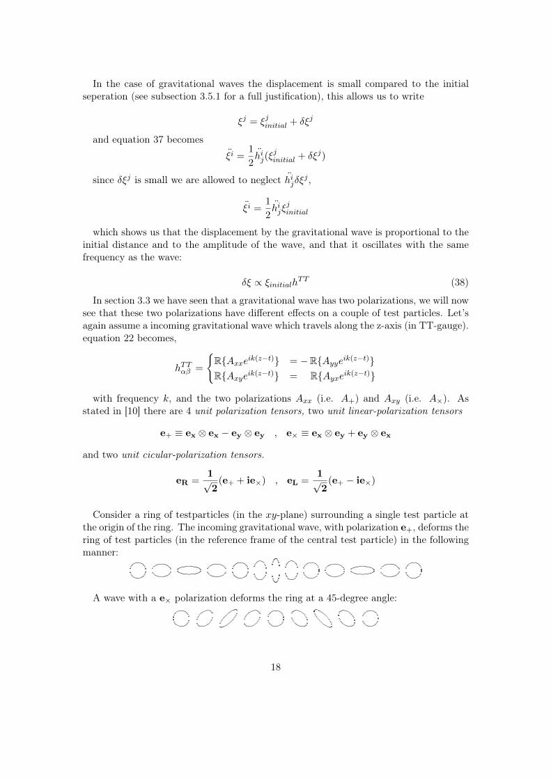
Consider a ring of testparticles (in the xy-plane) surrounding a single test particle atthe origin of the ring. The incoming gravitational wave, with polarization e+, deforms thering of test particles (in the reference frame of the central test particle) in the followingmanner:

A wave with a e× polarization deforms the ring at a 45-degree angle:

18

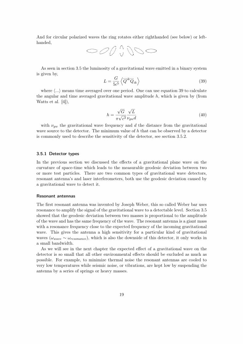
And for circular polarized waves the ring rotates either righthanded (see below) or left-handed,

As seen in section 3.5 the luminosity of a gravitational wave emitted in a binary systemis given by,

L =G

5c5

�...Q

ik...Qik

�(39)

where �...� means time averaged over one period. One can use equation 39 to calculatethe angular and time averaged gravitational wave amplitude h, which is given by (fromWatts et al. [4]),

h =

√G

π

√c3

√L

νgwd(40)

with νgw the gravitational wave frequency and d the distance from the gravitationalwave source to the detector. The minimum value of h that can be observed by a detectoris commonly used to describe the sensitivity of the detector, see section 3.5.2.

3.5.1 Detector types

In the previous section we discussed the effects of a gravitational plane wave on thecurvature of space-time which leads to the measurable geodesic deviation between twoor more test particles. There are two common types of gravitational wave detectors,resonant antenna’s and laser interferometers, both use the geodesic deviation caused bya gravitational wave to detect it.

Resonant antennas

The first resonant antenna was invented by Joseph Weber, this so called Weber bar usesresonance to amplify the signal of the gravitational wave to a detectable level. Section 3.5showed that the geodesic deviation between two masses is proportional to the amplitudeof the wave and has the same frequency of the wave. The resonant antenna is a giant masswith a resonance frequency close to the expected frequency of the incoming gravitationalwave. This gives the antenna a high sensitivity for a particular kind of gravitationalwaves (ωwave ∼ ωresonance), which is also the downside of this detector, it only works ina small bandwidth.

As we will see in the next chapter the expected effect of a gravitational wave on thedetector is so small that all other environmental effects should be excluded as much aspossible. For example, to minimize thermal noise the resonant antennas are cooled tovery low temperatures while seismic noise, or vibrations, are kept low by suspending theantenna by a series of springs or heavy masses.

19

Laser interferometers

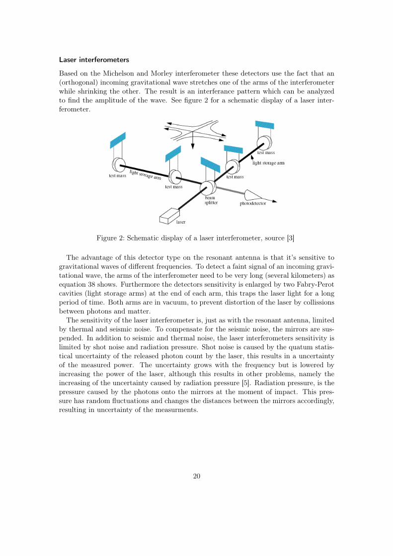
Based on the Michelson and Morley interferometer these detectors use the fact that an(orthogonal) incoming gravitational wave stretches one of the arms of the interferometerwhile shrinking the other. The result is an interferance pattern which can be analyzedto find the amplitude of the wave. See figure 2 for a schematic display of a laser inter-ferometer.

Figure 2: Schematic display of a laser interferometer, source [3]

The advantage of this detector type on the resonant antenna is that it’s sensitive togravitational waves of different frequencies. To detect a faint signal of an incoming gravi-tational wave, the arms of the interferometer need to be very long (several kilometers) asequation 38 shows. Furthermore the detectors sensitivity is enlarged by two Fabry-Perotcavities (light storage arms) at the end of each arm, this traps the laser light for a longperiod of time. Both arms are in vacuum, to prevent distortion of the laser by collissionsbetween photons and matter.

The sensitivity of the laser interferometer is, just as with the resonant antenna, limitedby thermal and seismic noise. To compensate for the seismic noise, the mirrors are sus-pended. In addition to seismic and thermal noise, the laser interferometers sensitivity islimited by shot noise and radiation pressure. Shot noise is caused by the quatum statis-tical uncertainty of the released photon count by the laser, this results in a uncertaintyof the measured power. The uncertainty grows with the frequency but is lowered byincreasing the power of the laser, although this results in other problems, namely theincreasing of the uncertainty caused by radiation pressure [5]. Radiation pressure, is thepressure caused by the photons onto the mirrors at the moment of impact. This pres-sure has random fluctuations and changes the distances between the mirrors accordingly,resulting in uncertainty of the measurments.

20

3.5.2 Existing and future gravitational wave detecters

As mentioned in section 3.5.1 there are two kinds of gravitational wave detectors, resonantantennas and laser interferometers. For the detection of gravitational waves from LMXB’s(see section 4) a detector with a wide bandwith is required. Resonant antennas aretherefore not the preferred detectors for this kind of events, and although there areseveral resonant antennas operational at the moment, they will not be discussed.

All over the world there are operational laser interferometers trying to detect gravi-tational waves. Here follows a short list, including specifications and references to theprojects in question.

GEO 600

Is a German-British gravitational wave detector situated near Sarstedt, Germany. Con-stuction on the project began in 1995, it has two perpendicular arms with a length of600 meters each and is capable of detecting gravitational waves in the frequency rangebetween 50 and 1500 Hz. With a theoretical sensitivity of h ∼ 10−22

Hz−1/2 at a gravita-

tional wave frequency of 1 kHz. More information can be found at the GEO 600 projectwebsite: http://www.geo600.org

VIRGO

The construction on the VIRGO detector at Cascina (Italy) was finished in 2003 andis currently in operation. VIRGO’s arms have a length of 3 kilometres, a frequencyrange from 10 to 6000 Hz and reaches a sensitivity of h ∼ 3 × 10−23

Hz−1/2 at a

gravitational wave frequency of 1 kHz. More information can be found at the EGO(European Gravitational Observatory) project website: http://www.ego-gw.it

TAMA 300 & CLIO

Are both protoype gravitational wave detectors situated in the Kamioka mine in Japan,constructed to develope advanced technologies necessary for the future gravitational wavedetector LCGT. TAMA 300 has two arms of 300 meters while the CLIO detector has onlyarms of 100 meter each. TAMA 300 reaches a maximum sensitivity of h ∼ 10−21

Hz−1/2

at a gravitational wave frequency of 1 kHz, while CLIO has it’s maximum sensitivity ata gravitation wave frequency of 250 Hz, h ∼ 2.5× 10−19

Hz−1/2 [14]. More information

can be found at the TAMA project website: http://tamago.mtk.nao.ac.jp

LIGO

LIGO which stands for Laser Interferometer Gravitational-wave Observatory, is a collab-oration of three laser interferometer observatories in the United States, two situated nearRichland, Washington and one at Livingston, Louisiana. These three detectors have armlengths of 4, 2 and 4 kilometers respectively and are operational since the year 2002.

21

LIGO’s maximum sensitivity reached h ∼ 10−22Hz

−1/2 [1], before it was upgradedbetween 2007 and 2009 to the so called Enhanced LIGO, which aimed to double it’soriginal sensitivity, and concluded it’s run in 2010. LIGO is currently being upgradedfor the second time, to Advanced LIGO (see below).

In addition to the existing detectors, there are several projects planned for futuredetectors with even higher sensitivities and/or different frequency ranges. Three of theseproposed detectors are the LCGT the Advanced LIGO and the ET.

LCGT

The LCGT is a second generation gravitational wave detector which is currently beingconstructed in the Kamioka mine in Japan, and is planned to be operational in 2018[15]. The LCGT detector has two orthogonal arms of 3 km in length and reaches amaximum sensitivity of h ∼ 3 × 10−24

Hz−1/2 at a gravitational wave frequency of 100

Hz [2]. More information can be found at the LCGT project website: http://gw.icrr.u-tokyo.ac.jp/lcgt/

Advanced LIGO

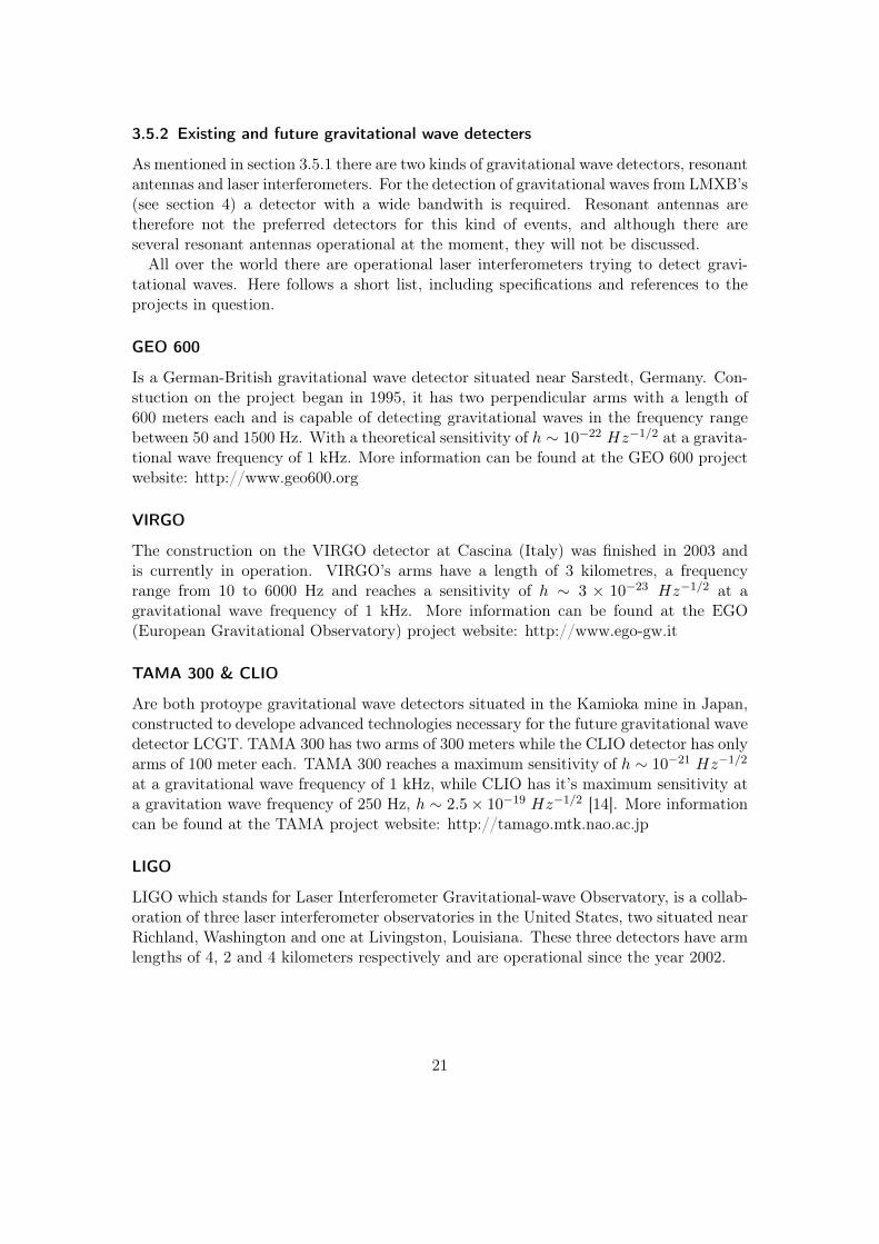
The upgrade of (Enhanced) LIGO to Advanced LIGO should be finished in 2014, makingit the first second generation gravitational wave detector in the world. The increase insensitivity is realised by rebuilding the whole detector, limiting every form (optical,thermal as well as seismic) of noise to a minimum. The predicted sensitivity curve isgiven below. More information can be found at the Advanced LIGO project website:https://www.advancedligo.mit.edu/

Figure 3: Theoretical sensitivity curve of Advanced LIGO, for an integration time of 2years.

The curves are obtained using data from Advanced LIGO website [1]. An explanationon how this graph is created can be found in Appendix 8.2.

22

ET

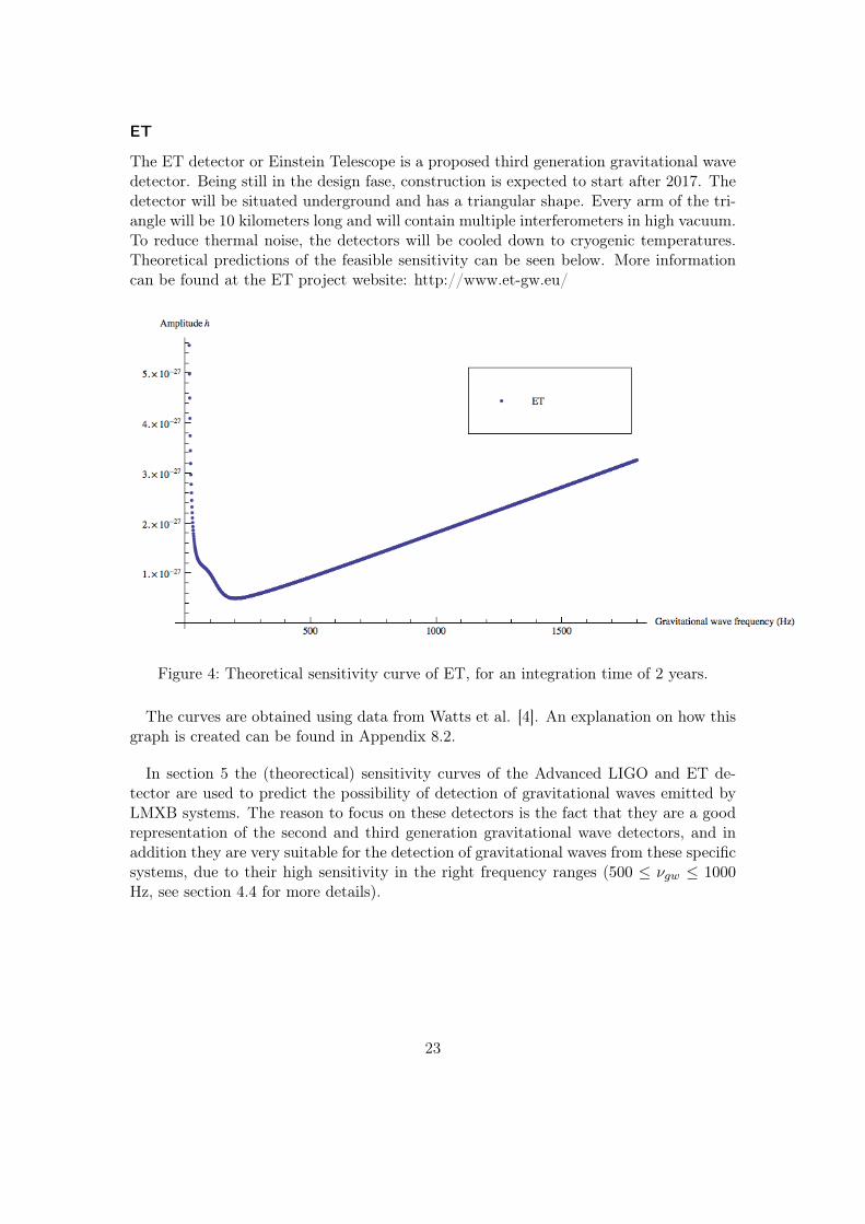
The ET detector or Einstein Telescope is a proposed third generation gravitational wavedetector. Being still in the design fase, construction is expected to start after 2017. Thedetector will be situated underground and has a triangular shape. Every arm of the tri-angle will be 10 kilometers long and will contain multiple interferometers in high vacuum.To reduce thermal noise, the detectors will be cooled down to cryogenic temperatures.Theoretical predictions of the feasible sensitivity can be seen below. More informationcan be found at the ET project website: http://www.et-gw.eu/

Figure 4: Theoretical sensitivity curve of ET, for an integration time of 2 years.

The curves are obtained using data from Watts et al. [4]. An explanation on how thisgraph is created can be found in Appendix 8.2.

In section 5 the (theorectical) sensitivity curves of the Advanced LIGO and ET de-tector are used to predict the possibility of detection of gravitational waves emitted byLMXB systems. The reason to focus on these detectors is the fact that they are a goodrepresentation of the second and third generation gravitational wave detectors, and inaddition they are very suitable for the detection of gravitational waves from these specificsystems, due to their high sensitivity in the right frequency ranges (500 ≤ νgw ≤ 1000Hz, see section 4.4 for more details).

23

4 Neutron stars

Neutron stars are the most compact stars known in the universe and are created as stellarremnants of massive stars at the end of their lives. The mass of a typical neutron star isof the same order as the mass of our Sun, Mneutronstar ∼ 1.4M⊙ [16] with M⊙ the Sun’smass (M⊙ = 1.9891×1030 kg). On the other hand the radius of a neutron star is onlyR ∼ 10 km. This results in an extremely high (average) density of

ρ � 7× 1014 gcm−3 ∼ (2− 3)ρ0

where ρ0 = 2.8× 1014 gcm−3 is the so called “normal nuclear density”, the mass densityof nucleon matter in heavy atomic nuclei [16].

Formation

Most neutron stars are created in Type-II supernova explosions, where a massive star(10 M⊙ � M � 25 M⊙, [11]) collapses under it’s own gravitational force after nuclearfusion in the core ended. The core collapses to a neutron star and the outer layers ofthe star are blown away. The supernova explosion releases an enormous energy of about1053 erg, which consists of mostly neutrino’s and some electromagnetic radiation in thewhole range of the EM-spectrum [16]. During the collapse of the star’s core, most of itsangular momentum is retained, while the radius diminishes greatly, which results intovery high rotation speeds. The same holds true for the magnetic field of the collapsed star,since the strength of the magnetic field is proportional to 1/r2, it increases during thecollapse. After formation, neutron stars have rotation periods between 1.4 millisecondsto 30 seconds and typical magnetic fields of ∼ 1012 Gauss. The temperature of a newlyformed neutron star can be as high as 1012 Kelvin. However, copious amounts of emittedneutrino’s carry away much of this energy, rapidly cooling the neutron star down[17].

Radiation

Neutron stars radiate not only neutrinos but also electromagnetic radiation and some-times gravitational radiation (See subsection 4.4 and section5). Most neutrinos are gen-erated in the star’s core and dominate the stars cooling for the first 105 years. When theneutron star becomes older, thermal electromagnetic radiation takes over in the coolingprocess. The first neutron star has been observed in the sixties as a unusual bright radiosource. Later on, other discoveries showed that neutron stars can also radiate in theX-ray or even gamma ray band of the electromagnetic spectrum. Most of this electro-magnetic radiation is emitted along the axis of the magnetic field. It is possible thatthe magnetic axis isn’t aligned with the axis of rotation, this results in a signal whichappears, to the observer, as pulsating. Neutron stars that show this phenomenon arecalled pulsars.

24

4.1 Neutron star structure

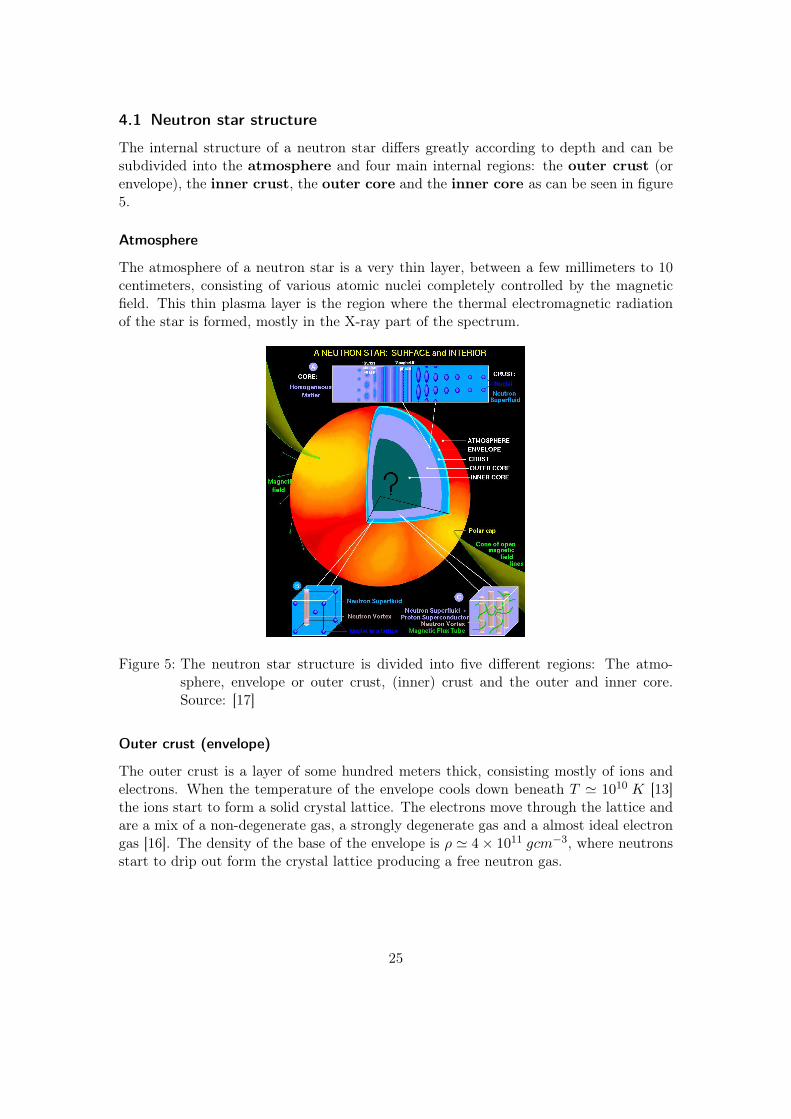
The internal structure of a neutron star differs greatly according to depth and can besubdivided into the atmosphere and four main internal regions: the outer crust (orenvelope), the inner crust, the outer core and the inner core as can be seen in figure5.

Atmosphere

The atmosphere of a neutron star is a very thin layer, between a few millimeters to 10centimeters, consisting of various atomic nuclei completely controlled by the magneticfield. This thin plasma layer is the region where the thermal electromagnetic radiationof the star is formed, mostly in the X-ray part of the spectrum.

Figure 5: The neutron star structure is divided into five different regions: The atmo-sphere, envelope or outer crust, (inner) crust and the outer and inner core.Source: [17]

Outer crust (envelope)

The outer crust is a layer of some hundred meters thick, consisting mostly of ions andelectrons. When the temperature of the envelope cools down beneath T � 1010 K [13]the ions start to form a solid crystal lattice. The electrons move through the lattice andare a mix of a non-degenerate gas, a strongly degenerate gas and a almost ideal electrongas [16]. The density of the base of the envelope is ρ � 4× 1011 gcm−3, where neutronsstart to drip out form the crystal lattice producing a free neutron gas.

25

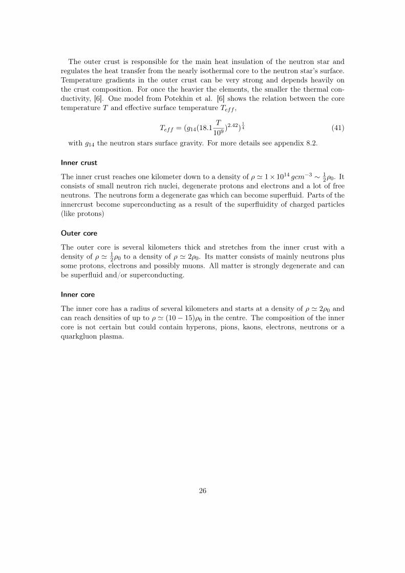
The outer crust is responsible for the main heat insulation of the neutron star andregulates the heat transfer from the nearly isothermal core to the neutron star’s surface.Temperature gradients in the outer crust can be very strong and depends heavily onthe crust composition. For once the heavier the elements, the smaller the thermal con-ductivity, [6]. One model from Potekhin et al. [6] shows the relation between the coretemperature T and effective surface temperature Teff ,

Teff = (g14(18.1T

109)2.42)

14 (41)

with g14 the neutron stars surface gravity. For more details see appendix 8.2.

Inner crust

The inner crust reaches one kilometer down to a density of ρ � 1× 1014 gcm−3 ∼ 12ρ0. It

consists of small neutron rich nuclei, degenerate protons and electrons and a lot of freeneutrons. The neutrons form a degenerate gas which can become superfluid. Parts of theinnercrust become superconducting as a result of the superfluidity of charged particles(like protons)

Outer core

The outer core is several kilometers thick and stretches from the inner crust with adensity of ρ � 1

2ρ0 to a density of ρ � 2ρ0. Its matter consists of mainly neutrons plussome protons, electrons and possibly muons. All matter is strongly degenerate and canbe superfluid and/or superconducting.

Inner core

The inner core has a radius of several kilometers and starts at a density of ρ � 2ρ0 andcan reach densities of up to ρ � (10− 15)ρ0 in the centre. The composition of the innercore is not certain but could contain hyperons, pions, kaons, electrons, neutrons or aquarkgluon plasma.

26

4.2 Neutron star types

Most of the description above is true for all neutron stars, but apart from all thesesimilarities there also exist a lot of differences between neutron stars. These differencesare used by astronomers to categorize the stars, firstly in two main categories:

• Single pulsars

• Binary pulsars

Single pulsars are either neutron stars which were formed from a single star or neutronstars which were created in a binary system, but eventually accreted their companioncompletely. Single pulsars can be subdivided, according to the source of the powerof the emitted electromagnetic radiation, in rotation powered pulsars and magnetars.Magnetars are neutron stars with extremely high magnetic fields (B � 1014 Gauss),which power the emittion of electromagnetic radiation. Rotation powered pulsars emitradiation powered by loss of rotational energy, this causes the stars to slow down.

The next section addresses binary systems, which are again subdivided in severaldifferent categories.

4.3 Neutron stars in binary systems

Neutron stars can be in all kinds of binary systems: with other neutron stars, with whitedwarfs or nondegenerate stars. All binary systems are divided into two classes: Widesystems and compact systems. In wide systems mass transfer is absent, and the starcan be considered as an isolated object. The focus of this thesis is on compact systems,where mass transfer from a companion to a neutron star leads to X-ray emissions; suchsystems are called X-ray binaries [16]. In these systems the mass transfer is a result ofthe gravitational pull of the neutron star, which strips (mostly gaseous) matter from thecompanion onto the accretion disk of the neutron star. The source of X-ray emissions iseither near the neutron star surface or the accretion disk, which is formed due to angularmomentum conservation. X-ray binaries are again divided in two sub-classes:

1. High-mass X-ray binaries (HMXBs, with M2 � (2− 3)M⊙)

2. Low-mass X-ray binaries (LMXBs, with M2 � M⊙)

With M2 the mass of the companion star, which is for HMXBs usually massive O-B starsand for LMXBs mostly dwarf stars (red dwarfs in particular).

Emission of electromagnetic radiation of X-ray binaries is powered by accretion butis not necessarily periodic. Some X-ray binaries show irregular emission and are calledX-ray transients, regular X-ray binaries are called: persistent.

27

X-ray transients

X-ray transients are: “X-ray sources which go from active (or on) to quiescent (or of)states and back on timescales of some hours and longer”. This behavior is caused by,“particularly, instabilities in the accretion disk, irregular outflow of matter from a donorstar, or by the changes of accretion regime near a neutron star surface” [16]. There aretwo types of X-ray transients:

1. Hard X-ray transients (HXTs) emit Hard X-rays (λ � 10−10 m) and are mostlyHMXBs.

2. Soft X-ray transients (SXTs) emit Soft X-rays (λ � 10−9 m) and are LMXBs.

X-ray pulsars

X-ray pulsars in compact binaries are a form of persistent X-ray sources which are pow-ered by accretion from a close companion. Due to the accretion the pulsar spin perioddecreases as the neutron star spins up. This is in contrast with the earlier discussedrotation powered pulsars in solitary systems, (which slowes down). However some X-raypulsars have been found to have reached a maximum rotation speed and undergo varia-tions around this equilibrium limit. One possible explanation for this phenomena is, aswe shall see later on, the loss of rotational energy due to gravitational wave emission.

X-ray bursters

X-ray bursters are identified as LMXBs and some of them show quasiperiodic X-rayoscillations (called QPOs) during their X-ray bursts. The X-ray bursts are formed onthe surface of the star and repeat quasiperiodically every several hours and last usuallyfrom a few seconds to a few tens of seconds. The bursts emit soft X-rays, much softerthan X-rays form pulsars.

“All X-ray bursts are subdivided into different parts:

1. Type I: Are widespread phenomena, and are explained by explosive thermonuclearburning of accreted matter on the surfaces of neutron stars with low magnetic fields(B � 108 − 109 Gauss).

2. Type II: Neutron stars in transiently accreting LMXBs. These bursts are veryfrequent and are associated with the nonstationary accretion onto a neutron star.

3. Superbursts: are rare events but very strong (Energy release can be several ordersof magnitude higher than in an ordinary X-ray burst). They are usually explainedby unstable carbon burning in deep layers of the outer crust of an accreting neutronstar” [16].

28

4.4 Gravitational wave emission

There are several ways for neutron stars (in binary systems) to emit gravitational waves,as mentioned in section 3.4, the only requirement for the emission of gravitational wavesis an accelerating non-spherical distribution of mass. The following configurations satisfythis requirement.

(Merging) binary systems

In every binary system where two unequal masses rotate around each other, there isemission of gravitational waves. In wide binary systems the gravitational wave signalhas a nearly constant frequency, proportional to the rotation speed of the two objects.The signal strength of these systems is proportional to the masses of the rotating objectsand inversely proportional to their distance.

Detection of gravitational waves from these systems is therefore most likely to occuronly for systems with black holes and moreover for merging systems, where rotationspeeds are very high.

Supernova explosions and star quakes

During a supernova explosions or starquake, great amounts of matter get accelerated,and since this happens mostly in a non-spherical manner, this results in the emissionof gravitational waves. These events happen very seldom and are often far away, whichmakes it hard to detect the gravitational waves. Luckely there is a big emission ofelectromagnetic radiation in these events as well, which can be detected and helps thesearch for gravitational waves.

Rotating neutron stars with non-spherical mass distributions

In the case that a neutron star (or any other rotating massive object) has a non-sphericalmass distribution, this results into a quadrupole moment. In combination with therotation of the star this results into the emission of gravitational waves. The strength ofthe gravitational wave is proportional to the quadrupole moment and the frequency ofthese emitted gravitational waves is twice the orbital frequency of the neutron star, [13].As long as the star rotates with a constant speed, a constant signal of gravitational wavescan be detected. One possible cause for a non-spherical mass distribution is accretion ofmatter from a companion star in a binary system (see section 5). Section 5.2 discussesthe possibility of detection from these systems.

The emission of gravitational waves results in energy loss of the binary system. RusselAlan Hulse and Joseph Hooton Taylor proposed that the emission of gravitational wavesis an explanation for the decrease in orbital period of the binary pulsar PSR B1913+16.This was the first indirect evidence for existence of gravitational waves and earned Hulseand Taylor the nobelprize in 1993.

29

5 Gravitational wave emission in LMXBs

This section will describe how gravitational waves emerge in LMXBs and discusses ifthe resulting gravitational wave signals are strong enough to be detected with second orthird generation gravitational wave detectors. In addition we will look if observation ofelectromagnetic radiation in transient systems can help to detect gravitational waves.

5.1 Quadrupole emergence

In section 4.4 we have seen that a non-spherical mass distribution in a neutron star isrequired in order for it to emit gravitational waves. This section will explain how such anon-spherical mass distribution can arise in a LMXB system.

5.1.1 Composition and temperature asymmetries through accretion

In a compact LMXB system, the gravitational pull of the neutron star results in amass transfer from the companion star, called accretion. Due to angular momentumconservation this (mostly gaseous) matter forms a accretion disc around the neutron star.Eventually the matter spirals down onto the surface of the neutron star were it pushesthe present matter down, again due to the gravitational pull. This gives rise to increasedpressure and temperatures, resulting in burning and (at higher densities/temperatures)nuclear reactions that change the composition of the neutron star.

According to Ushormirsky et al. [12] the composition of the matter entering the topof the crust of the neutron star depends on the burning conditions and accretion ratebut is still not well known. The presence of a weak magnetic field could affect the localaccretion rate resulting in a non-spherical symmetric distribution of accreted materialand changing the compostion of the neutron star locally. Positive feedback mechanisms(see below) could cause these asymmetries to grow and provide a possible explanationfor the existence of a compostion asymmetry. Since it’s impossible to compute themagnitude of these asymmetries from first principles, Ushormirsky et al. postulate aninitial composition asymmetry to further explore it’s consequences.

The result of a lateral composition asymmetry are temperature variations in the neutronstar crust, δT . There are two ways how these temperature variations are created.

1. Different elements have different charge-to-mass ratios (Z/A), which affect both thethermal conductivity and the neutrino emissivity. A lateral compostion asymmetrywill lead to lateral variations in the above transport properties causing lateraltemperature variations, δT .

2. Nuclear reactions in the crust, release energy and cause heat, which happens locally.Different elements release different amounts of energy in (different) nuclear reac-tions. Therefore, a lateral composition asymmetry will create another temperaturegradient through nuclear reactions.

30

As we have seen so far, a lateral composition asymmetry, caused by asymmetric accretionin a LMXB, results in temperature variations in the crust of the neutron star. The nextsection describes how these composition and temperature asymmetries result into a non-zero quadrupole moment.

5.1.2 Resulting quadrupole moment

The composition of a neutron star varies with depth, as the pressure increases when mov-ing toward the center of the star (see section 4.1).The pressure caused by the gravitationalforce is in equilibrium with the electron degeneracy pressure in the outer core and theelectron and neutron degenaracy pressure in the inner core. The dominant pressure inthe outer core aswell as in the inner core is the degenerate electron pressure.

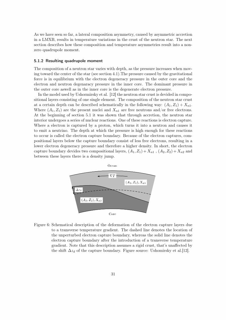
In the model used by Ushormirsky et al. [12] the neutron star crust is devided in compo-sitional layers consisting of one single element. The composition of the neutron star crustat a certain depth can be described schematically in the following way: (A1, Z1) +Xn1.Where (A1, Z1) are the present nuclei and Xn1 are free neutrons and/or free electrons.At the beginning of section 5.1 it was shown that through accretion, the neutron starinterior undergoes a series of nuclear reactions. One of these reactions is electron capture.Where a electron is captured by a proton, which turns it into a neutron and causes itto emit a neutrino. The depth at which the pressure is high enough for these reactionsto occur is called the electron capture boundary. Because of the electron captures, com-positional layers below the capture boundary consist of less free electrons, resulting in alower electron degeneracy pressure and therefore a higher density. In short, the electroncapture boundary devides two compositional layers, (A1, Z1)+Xn1 , (A2, Z2)+Xn2 andbetween these layers there is a density jump.

Figure 6: Schematical description of the deformation of the electron capture layers dueto a transverse temperature gradient. The dashed line denotes the location ofthe unperturbed electron capture boundary, whereas the solid line denotes theelectron capture boundary after the introduction of a transverse temperaturegradient. Note that this description assumes a rigid crust, that’s unaffected bythe shift ∆zd of the capture boundary. Figure source: Ushomirsky et al.[12].

31

Now if there is a compositional asymmetry caused by accretion and this leads to atransverse temperature gradient, as seen in the previous section, the compositional lay-ers will shift (See figure 6). The reason for the compositional layer shift is the fact thatelectron captures are dependent not only on local pressure but also on the local tempera-ture. Therefore it is possible for electron captures to occur even at higher altitudes thanthe former electron capture boundary, as long as the temperature is high enough.

Electron captures do occur at different altitudes in the neutron star crust, where everycapture boundary has it’s own threshold energy, Q. Shallow capture layers (above neu-tron drip) have threshold energies of ∼ 20 − 40MeV whereas deep capture layers (justabove the base of the inner crust) have threshold energies of ∼ 60− 100MeV .

Since the temperature variations in the NS crust are asymmetric, the resulting densityvariations due to “wavy” electron capture layers are also asymmetric which leads to anon-zero quadrupole moment. Ushomirsky et al.[12] used the following estimation tocalculate the quadrupole moment as function of the temperature deviation δT and thecapture layer threshold energy Q:

Q22 ≈ 1.3× 1037g cm2R

46

�δT

107K

��Q

30MeV

�3

(42)

where R6 = R/106cm, so for a typical neutron star radius R of 10 kilometer, R6 = 1.The above formula is only valid in the outer crust (Q � 40MeV ) and under the conditionthat the crust is non elastic, i.e there is no vertical readjustment of the crust.

Calculating the quadrupole moment for capture layers in the inner crust is more dif-ficult, this is caused by the fact that “the dependence of ∆zd and Q on the depth ismore complicated than in the outer crust because of the variation in number of electronscaptured and neutrons emitted in each capture layer” [12].

In addition to the quadrupole moment created by asymmetric temperature deviations,there is also a direct contribution to the quadrupole from the composition asymmetry.This quadrupole moment results from the deformation of the crust, caused by the differentelectron pressures from elements with different Z/A values. The next section will neglectthis direct contribution to the quadrupole and will focus only on the possible detectabilityof gravitational waves caused by asymmetrical temperature deviations in LMXBs.

5.2 Sensitivity measurements

The theoretical sensitivity curves of the Advanced LIGO and ET detectors are plottedin section 3.5.2. This section discusses what amount of temperature deviations in theneutron star crust are necessary to create strong enough gravitational waves in order todetect them with the detectors mentioned above. Let’s assume the existence of a typicalneutron star (in a LMXB system) with an avarage (i.e. unperturbed) crust temperature ofT = 108K and a radius of 10 kilometer at a distance of 5 kpc from earth, the integrationtime of the detectors is again 2 years.

32

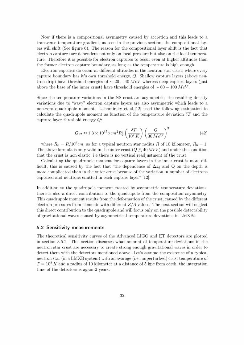
By using the model from Ushomirsky et al. [12] and assuming that all parametersdescribing the system (e.g. spinfrequency, distance, radius, etc.) are known, it is possibleto express the sensitivity curves of Advanced LIGO and ET in δT/T as function of thegravitational wave frequency in Hz. Figure 7 is created in this way (for details seeAppendix 8.2) where I introduced a single shallow capture layer with a threshold energyof 30 MeV in a neutron star with an unperturbed crust temperature of T = 108K anda radius of 10 kilometer at a distance of 5 kpc from earth, for an integration time of 2years.

Figure 7: Sensitivity curves of Advanced LIGO and ET expressed in δT/T as functionof the gravitational wave frequency in Hz. For a neutron star with a singleshallow ’wavy’ capture layer (Q = 30MeV ), an unperturbed crust temperatureof T = 108K and a radius of 10 kilometer at a distance of 5 kpc from earth,the integration time of the detectors is 2 years.

One can conclude from figure 7 that the detection of gravitational waves with the Ad-vanced LIGO detector is most likely at a gravitational wave frequency of a 1000 Hz. Thiscorresponds to a LMXB with a rotational frequency of 500 Hz, since νgravitationalwave =2× νrotation. There are X-ray bursters known that fit this description, a table of knowntransient systems can be found in an article by Watts et al. [4]. The detection of grav-itational waves from these sources, with the Advanced LIGO detector does require aminimal quadrupolar temperature deviation of 10 % (compared to the background tem-perature). Another possible source of gravitational waves are the kHz QPO sources (seesection 4.3) which have an average rotation speed of around 300 Hz [4]. The rotationspeeds of these systems are actually highly uncertain and model dependent, for the sakeof simplicity we will adopt νrot ≈ 300 Hz. Even with the more sensitive ET, detection isonly possible if the QPO sources have quadrupolar temperature asymmetries of ≥ 20%,wich is highly unlikely (see section 5.4).

33

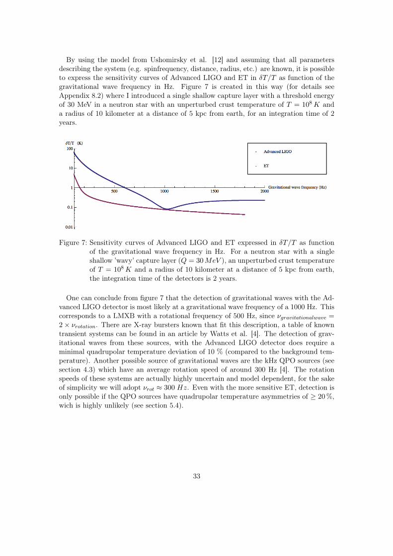
Figure 8 is an estimation of detection for a single deep capture layer with a thresholdenergy of 95 MeV, (all other parameters are the same as for the shallow capture layer, i.e.figure 7). The figure shows us that kHz QPO sources with rotation frequencies of 300 Hzand a deep capture layer with a temperature asymmetry of δT/T ≥ 0.05, can be detectedby the Advanced LIGO detector, and a temperature asymmetry of only δT/T ≥ 0.005 issufficient to create gravitational waves, detectable with the ET detector. X-ray bursterswith a rotational frequency of 500 Hz and a temperature asymmetry of δT/T ≥ 0.002,are likely to create detectable gravitational waves, for both detectors.

Figure 8: Sensitivity curves of Advanced LIGO and ET expressed in δT/T as functionof the gravitational wave frequency in Hz. For a neutron star with a singledeep ’wavy’ capture layer (Q = 95MeV ), an unperturbed crust temperatureof T = 108K and a radius of 10 kilometer at a distance of 5 kpc from earth,the integration time of the detectors is 2 years.

One can conclude from figure 7 and 8 that deep capture layers contribute more to theemission of gravitational waves than shallow ones. Moreover, detection of gravitationalwaves emitted by LMXBs is only probable in the case that there are several (deep) capturelayers present in the crust with a temperature asymmetry of at least a few percent.

5.3 Surface temperatures and X-ray modulations

This section shows the possibility of electromagnetic wave detections from transient sys-tems and how these detections can help the detection of gravitational waves. Section 5.1discussed how accretion in a LMXB can lead to temperature variations in the crust ofthe neutron star. These temperature variations will eventually reach the surface of theneutron star where they result in modulations in the electromagnetic wave emission ofthe neutron star. The observation of the modulations in the electromagnetic wave emis-sion on earth would give information on the temperature asymmetries on the surface ofthe neutron star. In combination with a good understanding of the thermal properties

34

of the neutron star crust it is possible to calculate the temperature asymmetries insidethe crust and predict the size of the quadrupole formation, without having to detect theactual graviational waves.

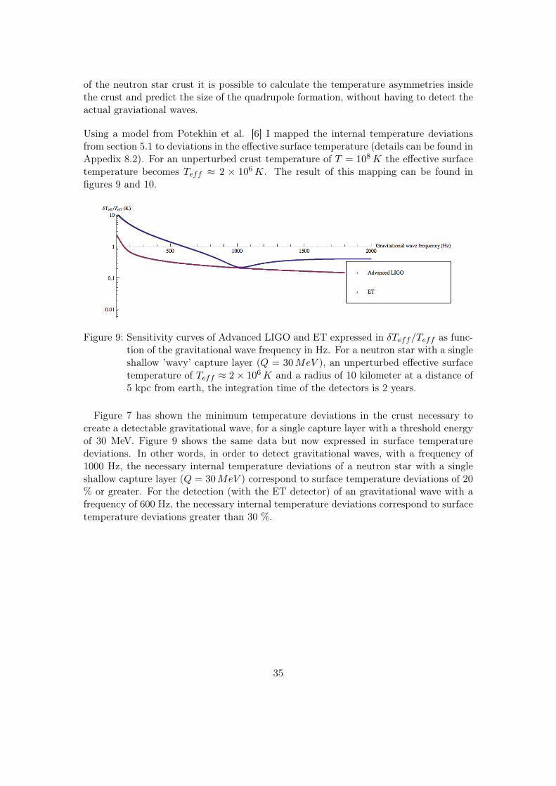
Using a model from Potekhin et al. [6] I mapped the internal temperature deviationsfrom section 5.1 to deviations in the effective surface temperature (details can be found inAppedix 8.2). For an unperturbed crust temperature of T = 108K the effective surfacetemperature becomes Teff ≈ 2 × 106K. The result of this mapping can be found infigures 9 and 10.

Figure 9: Sensitivity curves of Advanced LIGO and ET expressed in δTeff/Teff as func-tion of the gravitational wave frequency in Hz. For a neutron star with a singleshallow ’wavy’ capture layer (Q = 30MeV ), an unperturbed effective surfacetemperature of Teff ≈ 2× 106K and a radius of 10 kilometer at a distance of5 kpc from earth, the integration time of the detectors is 2 years.

Figure 7 has shown the minimum temperature deviations in the crust necessary tocreate a detectable gravitational wave, for a single capture layer with a threshold energyof 30 MeV. Figure 9 shows the same data but now expressed in surface temperaturedeviations. In other words, in order to detect gravitational waves, with a frequency of1000 Hz, the necessary internal temperature deviations of a neutron star with a singleshallow capture layer (Q = 30MeV ) correspond to surface temperature deviations of 20% or greater. For the detection (with the ET detector) of an gravitational wave with afrequency of 600 Hz, the necessary internal temperature deviations correspond to surfacetemperature deviations greater than 30 %.

35

These hot spots on the surface of the neutron star will modulate the intensity of theelectromagnetic wave emission from the surface. Due to the rotation of the neutron starwe could, theoretically speaking, see the hot spots as modulations in the electromagneticwave emission. In constant accreting systems, these modulations can’t be detected dueto the strong emission of electromagnetic waves in the accretion disk, which dominatesthe emission of all electromagnetic waves of the LMXB. In transient systems (e.g. burstoscillation sources or kHz QPO sources, see section 4.3) however, it is possible to detectthe modulations in the electromagnetic wave emission during the quiescent states of thesystem. In these states, accretion is temporarily halted and the thermal emission fromthe surface of the neutron star becomes the dominant contribution to the electromagneticradiation, making the modulations visible for detection.

Surface temperature deviations of 20 % might be big enough to be detected, whichcould used to test the probability of a single shallow capture layer causing gravitationalwaves. For instance if the measured surface temperature deviations are smaller than 20%, than it is impossible (using the model of Ushomirsky and Potekhin [12, 6]) to create aquadrupole big enough for detection with either the Advanced LIGO or the ET detector.

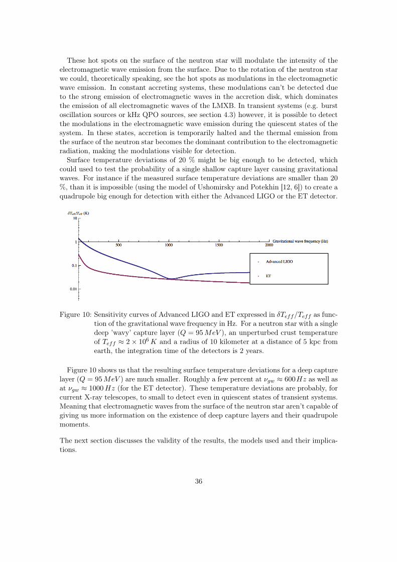
Figure 10: Sensitivity curves of Advanced LIGO and ET expressed in δTeff/Teff as func-tion of the gravitational wave frequency in Hz. For a neutron star with a singledeep ’wavy’ capture layer (Q = 95MeV ), an unperturbed crust temperatureof Teff ≈ 2× 106K and a radius of 10 kilometer at a distance of 5 kpc fromearth, the integration time of the detectors is 2 years.

Figure 10 shows us that the resulting surface temperature deviations for a deep capturelayer (Q = 95MeV ) are much smaller. Roughly a few percent at νgw ≈ 600Hz as well asat νgw ≈ 1000Hz (for the ET detector). These temperature deviations are probably, forcurrent X-ray telescopes, to small to detect even in quiescent states of transient systems.Meaning that electromagnetic waves from the surface of the neutron star aren’t capable ofgiving us more information on the existence of deep capture layers and their quadrupolemoments.

The next section discusses the validity of the results, the models used and their implica-tions.

36

5.4 Discussion

The evaluation of the results and the validity of the models used in section 5 will bediscussed in four seperate parts. Section 5.2 and section 5.3 are treated seperately, wheresection 5.2 is subdivided in two distinguishable cases, namely, a neutron star containing“shallow” or “deep” capture layers. But first, we will start of with a general evaluationconcerning every model used.

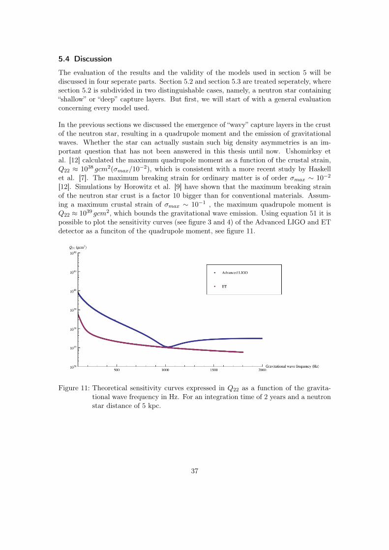
In the previous sections we discussed the emergence of “wavy” capture layers in the crustof the neutron star, resulting in a quadrupole moment and the emission of gravitationalwaves. Whether the star can actually sustain such big density asymmetries is an im-portant question that has not been answered in this thesis until now. Ushomirksy etal. [12] calculated the maximum quadrupole moment as a function of the crustal strain,Q22 ≈ 1038 gcm2(σmax/10−2), which is consistent with a more recent study by Haskellet al. [7]. The maximum breaking strain for ordinary matter is of order σmax ∼ 10−2

[12]. Simulations by Horowitz et al. [9] have shown that the maximum breaking strainof the neutron star crust is a factor 10 bigger than for conventional materials. Assum-ing a maximum crustal strain of σmax ∼ 10−1 , the maximum quadrupole moment isQ22 ≈ 1039 gcm2, which bounds the gravitational wave emission. Using equation 51 it ispossible to plot the sensitivity curves (see figure 3 and 4) of the Advanced LIGO and ETdetector as a funciton of the quadrupole moment, see figure 11.

Figure 11: Theoretical sensitivity curves expressed in Q22 as a function of the gravita-tional wave frequency in Hz. For an integration time of 2 years and a neutronstar distance of 5 kpc.

37

Figure 11 shows the possibility of detection of gravitational waves with the AdvancedLIGO and ET detectors. In the case of gravitational wave emission from neutron stars,detection with the ET detector is not affected by the boundary set by the crustal strainof the neutron star. For the Advanced LIGO, detection from LMXBs is only possiblefor a gravitational wave frequency of νgw � 200Hz. Since detection with the AdvancedLIGO for νgw � 200Hz requires a quadrupole moment bigger than the crust can sustain.Luckily this frequency region is of no real interest, since LMXBs emit gravitational wavesat higher frequencies (see table 1, form Watts et al. [4])

It is important to note that the fact that the neutron star crust can sustain a quadrupolemoment of only up to Q22 ≈ 1039 gcm2, does not mean that they have to be strained tothis maximum.

The results in section 5.2 and 5.3 are valid for LMXBs at a distance of 5 kpc from earth.However most LMXBs (Accreting millisecond pulsars, Burst oscillation sources and kHzQPO sources) are situated at a distance greater than 5 kpc (see table 1 in [4], from Wattset al.). As h is inversely proportional to the distance (see eqation 48), the possibility ofgravitational wave detection from most of the LMXB systems requires larger asymmetrictemperature deviations than mentioned in section 5.2.

In addition it is perfectly possible that the distance to the LMXB is uncertain, whichmight also hold for other parameters (e.g. the spinfrequency or the internal temperature).It is clear that the sensitivity of the detectors is reduced when there is an uncertainty inany of the systems parameters (Watts et al. [4]). The actual results; figure 7 and 8 areideal cases where all the parameters are known. It is important to remember that this isan exceptional case.

To create the figures 7 and 8 equation 42 was used. Which assumes a rigid crust. Ac-cording to Ushormirsky et al. [12] a better approximation of the quadrupole momentis achieved when using a model that allows for elastic deformation of the crust. “Thecrust prefers to sink in response to the shift in capture layers, and this reduces the actualquadrupole moment significantly” [12]. The results are different for different capturelayers and are discussed seperately, see the subsections below.

One positive effect on the possibility of detection is that the results in section 5.2 and 5.3assume only single capture layers. The existence of several capture layers is possible andthis multiplicative factor increases the quadrupole moment and therefore the possibilityof detection.

Gravitational waves from shallow capture layers

As mentioned above, eqation 42 does not account for vertical readjustment of the neutronstar crust. Figure 15 in [12] from Ushomirsky et al. shows the so called “sinking penalty”caused by this vertical readjustment of the crust. In this model, where the neutronstar interior is treated as an elastic solid, the resulting quadrupole for a shallow capturelayer reduces by a factor 20-50. This sinking penalty may reduce the possibility ofdetection from shallow capture layers even more, demanding (quadrupolar) temperature

38

asymmetries of more than 100%. It is impossible to believe that such large temperatureasymmetries can emerge, using (only) the models in this thesis.

Gravitational waves from deep capture layers

The sinking penalty for a deep capture layer is considerably smaller, according to Ushomirskyet al [12] the quadrupole moment reduces by a factor 5-10.

There is an additional statement concerning the calculations of the quadrupole momentof a deep capture layer. The used approximation (eqation 42) is only valid for shallowcapture layers, see section 5.1.2. Figure 14 in [12], from Ushomirsky et al., shows adeviation in Q22 of a factor ∼ 10 with respect to equation 42. When including thesinking penalty for both the models. For a temperature deviation of δT ∼ 2%, thequadrupole moment is 10 times bigger that equation 42 suggests.

It is therefore safe to assume that the temperature deviations required for the detec-tion of gravitational waves from deep capture layers (as presented in figure 8) are quiteaccurate, since the factor of 5-10 (due to the sinking penalty) cancel out the fault (withinan order of magnitude) in equation 42.

The asymmetric temperature deviations necessary for detection, in the case of a singledeep capture layer, as discussed in section 5.2 can be considered realistic. As Ushormirskyet al. [12] show that a 10 % laterally varying energy or charge to mass ratio, can resultin temperature asymmetries of a few percent (see figure 8 in [12]).

Surface temperature deviations

The surface temperature deviations, as depicted in figure 9 and 10, are calculated using amodel from Potekhin et al. [6]. This paper describes the insulating effect of the envelopeof an accreting neutron star and proposes a model for the relation between the internaltemperature Tb and the effective surface temperature Teff . Where Tb is the temperaturenear the base of the envelope at a density of ρb = 1010 gcm

−3. Both the shallow as

the deep capture layer are located deeper in the star at densities of ∼ 1011 gcm−3 and∼ 1014 gcm

−3, respectively. Which raises the question whether the model is valid inour case. However as stated before, the envelope is the main insulation of the neutronstar, and the internal crust temperature can be considered fairly constant. As figure 7of Ushormirsky et al. [12] confirms (the temperature difference over the pressure range1025 ≤ P ≤ 1033 with P in ergcm

−3 is less than a factor 2). This validates the use ofequation 53 as our typical neutron star satisfies the other conditions (as mentioned insection 8.2) as well.

39

6 Conclusion & Outlook

Section 5 has shown us the possibilities of detecting gravitational waves from LMXBswith single (shallow or deep) capture layers with the Advanced LIGO and ET detector,as well as the size of the resulting surface temperature deviations originating from thesecapture layers. As discussed in section 5.4 the results are for a purely ideal case whereall parameters are known, the crust is infinitely rigid and the neutron star is at a rela-tively short distance from earth. Through looking at the consequences of a model fromUshomirsky et al. [12], where the neutron star crust is considered as an elastic solid withan maximum breaking strain of σ ∼ 10−1 (from Horowitz et al. [9]), we can adjust ourfindings on the possibility of detecting gravitational waves from these systems.

It is safe to conclude that the detection of gravitational waves with a frequencyνgw � 200 Hz is impossible with the Advanced LIGO detector, even if the crust ismaximally strained. Moreover we can rule out any gravitational wave detection (witheither the Advanced LIGO or the ET detector) from multiple “shallow” capture layers(Q � 40 MeV ), due to the large sinking penalty reducing the quadrupole moment bya factor 20-50 [12]. Since detection requires quadrupolar temperature deviations muchhigher than can be expected to be caused by accretion alone.

The existence of several “deep” capture layers (e.g. Q = 95 MeV ) could lead togravitational wave detection, since the sinking penalty is relatively small; a factor 5-10 [12]. The existence of quadrupolar temperature deviations of a few percent, can beconsidered possible according to Ushomirsky et al. [12] and are sufficient for detectionwith the Advanced LIGO detector (for νgw � 800 Hz) or with the ET detector (forνgw � 100Hz).

The internal temperature deviations in the neutron star crust, caused by accretion willlead eventually to temperature deviations on the surface. In combination with the ro-tation of the neutron star this will result in modulations of the X-ray flux. Section 5.3shows that the presence of a “deep” capture layer, required for gravitational wave de-tection, will result in effective surface temperature deviations of only a few percent inthe case of the Advanced LIGO detector (for νgw � 800 Hz) or the ET detector (forνgw � 100 Hz). These surface temperature deviations are most likely to small to bedetected as modulations in the X-ray flux, even in quiescent states.

However, it might be possible to detect X-ray modulations from “shallow” capturelayers, even though it is impossible to detect the gravitational waves from these capturelayers, since they are to weak. As section 5.3 shows, can temperature deviations of 10% at a “shallow” capture layer (Q = 30 MeV ) result in effective surface temperaturedeviations of 20 %. Surface temperature deviations of this size might be big enough tobe detected as modulations in the X-ray flux, although further research in this area inrequired to confirm this.

The detection of these X-ray modulations in transient systems could confirm or excludethe existence of “shallow” capture layers in LMXBs and could provide information aboutthe size of the temperature deviations located in the neutron star’s internal.

40

Outlook

Whether the Advanced LIGO or ET detector will detect gravitational waves form LMXBsin the future has still to be seen. However, further improvements in determing thenecessary parameters of the LMXBs and further development on models of neutron starinteriors will lead to more precise predictions whether gravitational wave detection fromLMXBs is possible. More understanding of the neutron star interior will furthermore leadto better predictions on the surface temperature (deviations). In combination with moreprecise detections of electromagnetic wave modulations in transient systems this mightlead to the confirmation of the existence of temperature asymmetries (and thereforea quadrupole moment) in the neutron star, without requiring the direct detection ofgravitational waves.

Eventually, the detection of gravitational waves could lead to a better understandingof the LMXBs and open a new window for investigating the interior of neutron stars.

7 Acknowledgements

I would like to thank Brynmor Haskell for his supervision and patience during this project.Furthermore I want to thank Bouwe Andela for helping me understand the mathemat-ics behind General Relativity and Wieger Steggerda for helping me with programmingrelated questions. Finally I want to thank all other friends and family for their help andsupport.

Manuel Oppenoorth

41

8 Appendices

• 8.1 Mathematics and notations for General Relativity

• 8.2 Details on computations, simulations and graphics

8.1 Mathematics and notations for General Relativity

General Relativity is a geometric theory which describes the effects of matter on thecurvature of space-time. The notation and mathematics needed to describe curvatureare therefore geometric identities. In particular non-Euclidean geometry, which is incontrast with our normal sense of geometry (which is Euclidean). In Euclidean geometryare lines, distances, angles and relations between vectors and derivatives far more trivialthan in non-Euclidean geometry.

8.1.1 Einstein summation

To keep notations and calculations short and clear the Einstein summation convention isapplied. Greek indices can take on any value 0, 1, 2 or 3. In contrast with latin indiceswhich can only take on the values 1, 2, 3.

Einstein summation convention: Any index that is repeated in a product is automati-cally summed on:

xβyβ ≡

3�

β=0

xβyβ.

With xβ and yβ contravariant and covariant tensors respectively, both of order 1. See

section 8.1.2 for more on tensors.

As stated in the book Gravitation [10], “the positions of the indices in the lorentztransformation laws need not to be remembered if one only remembers the 2 followingrules:

1. Free indices ( indices not summed over) on each side of the equation are in thesame position.

2. Summed indices appear once up once down.”

42

8.1.2 Tensors

As mentioned in section 2.1, General Relativity requieres us to have indentities that areindependent of the choice of coordinate system. This can be achieved by the use oftensors. A tensor is a more general version of the vector as known in three dimensionalspace and represents relations between scalars, vectors and other tensors. There aremany kinds of tensors which can be distinguished by type(n,m) and order, where theorder of a tensor is given by n +m. The n stands for the upper index of a tensor (Tn)and the m for the lower index of a tensor (Tm). The position of the indices (either up ordown) determine how a object changes under a coordinate transformation. In general, atensor T (n,m) is a function which maps n vectors and m one-forms to a scalar. Tensorswith upper indices are called contravariant tensors whereas tensors with lower indicesare called covariant. Examples:

• Tensor type(0, 0) = scalar.

• Tensor type(1, 0) = (contravariant)vector.

• Tensor type(0, 1) = covariantvector or one-form.

• Tensor type(0, 2) = metric.

Tensors can either be symmetric or anti-symmetric:

• A symmetric tensor stays the same under interchanging of two indices i.e.

Tαβγ = T

βαγ

• An antisymmetric tensor changes sign under interchanging of two indices

Tαβγ = −T

βαγ

8.1.3 Metric tensor

A special form of tensor is the metric tensor g, which describes the “distances” betweenelements of a given set and therefore describes the geometry of the set. The metric tensoris a symmetric tensor, i.e. gαβ = gβα.

It is a machine with two input slots for the insertion of two vectors:g( , ). If one inserts two different vectors, u and v one gets a scalar which we define

as the scalar product of u and v:

g(u,v) = g(v,u) = u · v = v · u =gαβuαvβ

If one inserts the same vector u into both slots, one gets the square of the length of u:g(u,u) =� u �2.

43

The inverse metric is defined by:

gαγgγβ = δ

βα (43)

where δβαis the Kronicker delta, i.e:

δβα = {1 if α=β

0 otherwise

In spacetime the distance between two points is given by the infinitesimal element ds

with length,ds ≡

�gαβdx

αdxβ

For Minkowski space, i.e. flat spacetime the metric looks like:

gαβ = ηαβ =

−1 0 0 00 1 0 00 0 1 00 0 0 1

where α labels the rows and β the columns of the matrix.The minkowski metric tensor is its own inverse metric tensor, i.e.

ηαβηαβ =

−1 0 0 00 1 0 00 0 1 00 0 0 1

−1 0 0 00 1 0 00 0 1 00 0 0 1

=

1 0 0 00 1 0 00 0 1 00 0 0 1

≡ I.

8.1.4 Tensor operations

The operation of applying a contravariant tensor with a covariant tensor is called tensorcontraction, and reduces the tensor rank by 2. Which is useful for many operationsbetween tensors, for example it can be used to lower or raise indices on any given tensor.To lower or raise a index of a tensor, one only has to contract it with the metric or theinverse metric respectively:

gαβxα = xβ .

It is often very useful to rewrite a tensor in such a way that they create anothertensor which is either symmetric or anti-symmetric, this is called symmetrizing andantisymmetrizing respectively.

Symmetrizing the symmetric tensor F (in αβ) to produce a symmetric tensor H canbe done as follows:

Hαβ = F(αβ) =1

2(Fαβ + Fβα).

And antisymmetrizing an antisymmetric tensor F (in αβ) to produce a antisymmetrictensor G is achieved like this:

Gαβ = F[αβ] =1

2(Fαβ − Fβα).

44

• The trace of a tensor is the sum of the elements on the main diagonal and can befound by contraction with the metric. I.e. Trace F

αβ = gαβFαβ = F

ββ = F . The

trace of the metric is for example: gαβgαβ = g

ββ = δ

ββ = 4

• The derivative operator ∂∂xα can be written in short as ∂α. And the d’Albertian

operator as ∂∂xα

∂∂xα

≡ ∂α∂α ≡ �. But the derivative operator can also be written

even shorter, like this: ∂αTαβ ≡ T

αβ,α.

• The covariant derivative operator ∇γTαβ can be written as: Tαβ ; γ. And raises the

rank of the tensor by 1. Covariant derivative of a function solely of the metric isalways zero. The divergence of a tensor Tαβ can be written as: ∇α · Tαβ = T

αβ ;α

8.2 Details on computations, simulations and graphics

This appendix shows in short how the graphs in section 5 are created using models andcalculations from Ushomirksy [12], Watts [4] and Potekhin [6]. All calculations are donenumerically using the program Wolfram Mathematica® 8 for students.

Gravitational wave amplitude h

Section 3.4 showed that the luminosity of the emission of gravitational waves from abinary system is given by the quadrupole moment in the following way,

L =G

5c5

�...Q

ik...Qik

�(44)

With the quadrupole tensor Qik given by, Qik =

�ama(diad

ka − 1

3δikd2) and the dots

referring to time derivatives. One can calculate the quadrupole moment using a littlealgebra (from Ushomirsky et al. [12]), resulting in

�...Q

ik...Qik

�=

256π7Q

222ν

6gw

15(45)

where νgw is the gravitational wave frequency and Q22 is the (leading component ofthe) quadrupole moment. By filling equation 45 in to equation 44 we end up with thefinal form of the luminosity,

L =256π7

GQ222ν

6gw

75c5(46)

In section 3.5 it was shown that the time and angular averaged graviational wave ampli-tude as measured by a detector on earth is given by,

h =

√G

π

√c3

√L

νgwd(47)

with d the distance between the gravitational wave source and the detector.

45

Equation 47 can be rewritten by inserting the luminosity equation 46, resulting in

h =16

5

�π

3

GQ22π2ν2gw

dc4(48)

Equation 48 describes the strength of the measured gravitational wave on earth, emit-ted by an binary system with quadrupole moment Q22 and a rotational frequency ofνrotational at a distance d. Where the rotational frequency is given by the equationνrotational =

12νgw.

Sensitivity Curves

The sensitivity curves of the Advanced LIGO and ET detector in section 5 are createdusing data files from Watts et al. [4] and the Advanced LIGO website [1]. “The sensitivityof a GW detector is determined by the power spectral density of its instrumental strainnoise, normalized to an equivalent gravitational wave amplitude h(t). This is just theFourier power spectrum of h(t) and is called Sh(ν): the noise power per unit frequency.”[4] The two files (one for Advanced LIGO and one for the ET) were used to createthe sensitivity curves and existed of arrays of frequency ν and noise power per unitfrequencySh(ν) values.

In order to convert them to our conventional h (time and angular averaged gravitationalwave amplitude) the following formulae (49 and 50) were used,

h0 ≈ 11.4×�

Sh

Dt(49)

with D the number of detectors (in our case 1) and t the integration time in seconds(in our case 2 years). Equation 49 is only valid under the assumption that all parametersdescribing the system (e.g. spinfrequency, distance, etc.) are known. Any uncertainty inthe parameters reduces the sensitivity of the detector. Formula 49 is from Watts et al.[4] and calculates h0 rather than h. In order to get h the second formula is used,

h =

�2

5h0 (50)

By using the acquired h from the data files and rewriting equation 48 to,

Q22 =5hdc4

16�

π3Gπ2ν2gw

(51)

I calculated the sensitivity of Advanced LIGO and the ET expressed as the minimalquadrupole moment Q22 possible to detect as a function of the frequency ν. In section5.1.2 we adopted the model from Ushomirsky et al. [12] to describe how temperatureasymmetries can lead to a quadrupole moment. By rewriting their equation 42 to

δT =Q22

1.3× 1037107

R46

�30 MeV

Q

�3

(52)

46

it is now possible to plot the sensitivity of Advanced LIGO and the ET expressed inδT/T as seen in figures 7 and 8. The used (unperturbed) internal crust temperature wasT = 108K.

Surface temperature mapping

To create the figures 9 and 10, I used a model from [6] to map the internal crust tem-peratures T to effective surface temperatures Teff . The effective surface temperature isgiven by,

Teff = (g14(18.1T

109)2.42)

14 (53)

with g14 the surface gravity of the neutron star divided by 1014. Which is given by,

g14 =GM

�R

�1− (2GM/c2)/R

�2 × 10−14 (54)

and for a typical neutron star,

g14 ≈ 3.17 cms−2

Equation 53 is valid under the following conditions:

• 4.7 ≤ log Teff ≤ 6.5

• 0.4 ≤ log g14 ≤ 6

• Tb ≤ 108K

47

References

[1] Project website of LIGO [online]. November 2011. Available from:https://www.advancedligo.mit.edu/summary.html [cited november 14, 2011].

[2] Project website of the LCGT [online]. November 2011. Available from:http://gw.icrr.u-tokyo.ac.jp/lcgt/ [cited november 9, 2011].

[3] www.wikipedia.org on gravitational wave detector [online]. October 2011. Availablefrom: http://en.wikipedia.org/wiki/Gravitational_wave_detector.

[4] L. Bildsten A. L. Watts, B. Krishnan and B. F. Schutz. Detecting gravitationalwave emission from the known accreting neutron stars. Mon. Not. R. Astron. Soc.,389(2):839–869, 2008.

[5] B. Andela. Gravitational waves from X-ray bursts and superbursts. Mas-ter’s thesis, University of Amsterdam, October 2011. Available from:http://staff.science.uva.nl/∼bandela/gr_master_thesis.pdf.

[6] D. G. Yakovlev A.Y. Potekhin, G. Chabrier. Internal temperatures and cooling ofneutron stars with accreted envelopes. Astron. and Astrophys., 323:415–428, 1997.

[7] D. I. Jones B. Haskell and N. Andersson. Mountains on neutron stars: accretedversus non-accreted crusts. Monthly Notices of the Royal Astronomical Society,373:1423–1439, 2006.

[8] Artist: Dana Berry. Picture on frontpage [online]. December 2011. Available from:http://www.esa.int/esaCP/SEMWSAA5QCE_index_1.html.

[9] K. Kadau C. J. Horowitz. Breaking strain of neutron star crust and gravitationalwaves. Physical Review Letters, 102(1102), 2009.

[10] J.A. Wheeler C. W. Misner, K.S. Thorne. Gravitation. Freeman and Company,1973.

[11] G. Gilmore. The short spectacular life of a superstar. Science, 304(5679):1915–1916,June 2004.

[12] Curt Cutler Greg Ushomirsky and Lars Bildsten. Deformations of accreting neutronstar crusts and gravitational wave emission. Monthly Notices of the Royal Astro-

nomical Society, 319(3), 2000.

[13] B. Haskell. Gravitational Waves from Deformed Rotating Neutron Stars. PhD thesis,University of Southampton, 2007.

[14] D. Tatsumi K. Izumi Y. Wakabayashi H. Ishizaki M. Fukushima T. YamazakiM-K Fujimoto A. Takamori K. Tsubono R. DeSalvo A. Bertolini S. MarkaV. Sannibale T. Uchiyama O. Miyakawa S. Miyoki K. Agatsuma T. Saito M.

48

Ohashi K. Kuroda I. Nakatani S. Telada K. Yamamoto T. Tomaru T. Suzuki T.Haruyama N. Sato A. Yamamoto T. Shintomi K. Arai, R. Takahashi. Status ofjapanese gravitational wave detectors. Classical and Quantum Gravity, 26(20),2009. Available from: http://iopscience.iop.org/0264-9381/26/20/204020/pdf/0264-9381_26_20_204020.pdf.

[15] K. Kuroda. Status of LCGT. Classical and Quantum Gravity, 27, 2010.

[16] D.G. Yakovlev P. Haensel, A.Y. Potekhin. Neutron stars 1: Equation of State and

Structure, volume 326. Springer, New York, 2007.

[17] University of Maryland Prof M. Coleman Miller. Introductionto neutron stars. [online]. September 2011. Available from:http://www.astro.umd.edu/∼miller/nstar.html.

49