November 6, 2016

Graphs 1: Representation, Search, and Traverse

This notes chapter begins with a review of graph and digraph concepts and terminol-ogy and introduces the adjacency matrix and adjacency list representation systems.Then we study the depth-first and breadth-first search processes and elaborations onthem, including DFS and BFS traversals and the ultimate Survey algorithms.

Outside the Box

Best Lecture Slides PUBest Video UCBDemos DFSurvey (undirected) LIB/area51/fdfs ug.x

DFSurvey (directed) LIB/area51/fdfs dg.x

BFSurvey (undirected) LIB/area51/fbfs ug.x

BFSurvey (directed) LIB/area51/fbfs dg.x

Textbook deconstruction. This notes chapter corresponds roughly toChapter 22 in [Cormen et al 3e], which covers graph (and digraph) conceptsand representations and the basic depth- and breadth-first search processes.The notation G = (V, E) is common to the text, the video linked here, andthese notes.

1 Definitions, Notation, and Representations

Graphs and directed graphs are studied extensively in the pre-requisit math se-quence Discrete Mathematics I, II [FSU::MAD 2104 and FSU::MAD 3105], so thesenotes will not dwell on details. We will however mention key concepts in order toestablish notation and recall familiarity. Where there may be slight variations interminology, we side with the textbook (see [Cormen::Appendix B.4]). Assume thatG = (V, E) is a graph (directed or undirected).

1.1 Undirected Graphs - Theory and Terminology

• Undirected Graph: aka Ungraph, Bidirectional Graph, Bigraph; Graph• Vertices, vSize = |V | = the number of vertices of G• Edges, eSize = |E| = the number of edges of G.• Adjacency: Vertices x and y are said to be adjacent iff [x, y] ∈ E.• Path from v to w: a set x0, . . . , xk of vertices such that x0 = v, xk = w, and

[xi−1, xi] is an edge for i = 1, . . . , k. The edges [xi−1, xi] are called the edgesof the path and k is the length of the path. A path is simple if the vertices

1

2

defining it are distinct - that is, not repeated anywhere along the path. If pis a path from v to w we say w is reachable from v.

• Connected Graph: for all vertices v, w ∈ V , w is reachable from v.• Cycle: A path of length at least 3 from a vertex to itself.• Acyclic Graph: Graph with no cycles• Degree of a vertex v: deg(v) = the number of edges with one end at v.

1.2 Directed Graphs - Theory and Terminology

• Directed Graph: aka Digraph• Vertices, vSize = |V | = the number of vertices of G• Edges, eSize = |E| = the number of (directed) edges of G.• Adjacency: Vertex x is adjacent to vertex y, and y is adjacent from x, iff

(x, y) ∈ E.• Path from v to w: a set x0, . . . , xk of vertices such that x0 = v, xk = w, and

(xi−1, xi) is an edge for i = 1, . . . , k. The edges (xi−1, xi) are called the edgesof the path and k is the length of the path. A path is simple if the verticesdefining it are distinct - that is, not repeated anywhere along the path. If p isa path from v to w we say w is reachable from v. Note: that these edges areall directed and must orient in the forward direction.

• Strongly Connected Digraph: for all vertices v, w ∈ V , w is reachable from v.Note this means the existence of two directed paths - one from v to w andthe other from w to v. Also note that putting the two paths together createsa (directed) cycle containing both v and w.

• (Directed) Cycle: A path of length at least 1 from a vertex to itself. Notethis is distinct from the undirected case, allowing paths of length 1 (so-calledself-loops) and length 2 (essentially and out-and-back path, equivalent to atwo-way edge).

• Acyclic Digraph: Digraph with no cycles; DAG• inDegree of a vertex v: inDeg(v) = the number of edges to v.• outDegree of a vertex v: outDeg(v) = the number of edges from v.

There are subtle distinctions in the way graphs and digraphs are treated in definitions.There are also “conversions” from graph to digraph and digraph to graph.

• Undirected graph edges have no preferred direction and are represented usingthe notation [x, y] to mean the un-ordered pair in which [x, y] = [y, x]. Di-rected graph edges have a preferred direction and are represented using thenotation (x, y) to mean the ordered pair in which (x, y) 6= (y, x). (In practice,the notation [x, y] is often dropped when context makes it clear whether theedge is directed or undirected or when both directed and undirected graphsare considered in the same context.)

3

• In an undirected or directed graph, vertex y is said to be a neighbor of thevertex x iff (x, y) ∈ E. In undirected graphs, being neighbors and beingadjacent are equivalent. In digraphs, y is a neighbor of x iff y is adjacent fromx. (Note this terminology differs from that in [Cormen et al 3e].)

• If D = (V, E) is a digraph, the undirected version of D is the graph D′ =(V, E ′) where [x, y] ∈ E ′ iff x 6= y and (x, y) ∈ E. Note this replaces, ineffect, a 1-way edge with a 2-way edge (or two opposite 1-way edges in therepresentations), except self-loops are eliminated.

• If G = (V, E) is a graph, the directed version of G is the graph G′ = (V, E ′)where (x, y) ∈ E ′ iff [x, y] ∈ E. Note this replaces each undirected edge [x, y]with two opposing directed edges (x, y) and (y, x).

Theorem 1u. In an undirected graph,∑

v∈V deg(v) = 2× |E|.Theorem 1d. In a directed graph,

∑v∈V inDeg(v) =

∑v∈V outDeg(v) = |E|.

The proof of Theorem 1 uses aggregate analysis. First show the result for directedgraphs, where edges are in 1-1 correspondence with their initiating vertices. Thenapply 1d to the directed version of an undirected graph and adjust for the doublecounting.

1.3 Graph and Digraph Representations

There are two fundamental families of representation methods for graphs - connec-tivity matrices and adjacency sets. Two archetypical examples apply to graphs anddigraphs G = (V, E) with the assumption that the vertices are numbered startingwith 0 (in C fashion): V = v0, v1, v2, . . . , vn−1.

1.3.1 Adjacency Matrix Representation

In the adjacency matrix representation we define an n× n matrix M by

M(i, j) =

1 if G has an edge from vi to vj

0 otherwise

M is the adjacency matrix of G.

Consider the graph G1 depicted here:

0 --- 1 2 --- 6 --- 7Graph G1 | | |

| | |3 --- 4 --- 5 --- 8 --- 9

4

The adjacency matrix for G1 is:

M =

− 1 − 1 − − − − − −1 − − − − − − − − −− − − − − 1 1 − − −1 − − − 1 − − − − −− − − 1 − 1 − − − −− − 1 − 1 − − − 1 −− − 1 − − − − 1 − −− − − − − − 1 − − 1− − − − − 1 − − − 1− − − − − − − 1 1 −

(where we have used “−” instead of “0” for readability). Adjacency matrix repre-sentations are very handy for some graph contexts. They are easy to define, low inoverhead, and there is not a lot of data structure programming involved. And somequestions have very quick answers:

1. Using an adjacency matrix representation, the question “Is there an edge fromvi to vj ?” is answered by interpreting M(i, j) as boolean, and hence in timeΘ(1).

Adjacency matrix representations suffer some disadvantages as well, related to thefact that an n× n matrix has Θ(n× n) places to store and visit:

2. An adjacency matrix representation requires Θ(n2) storage.3. A loop touching all edges of a graph (or digraph) represented with an adja-

cency matrix requires Ω(n2) time.

Particularly when graphs are sparse - a somewhat loose term implying that the num-ber of edges is much smaller than it might be - these basic storage and traversal tasksshould not be so expensive.

1.3.2 Sparse Graphs

A graph (or digraph) could in principle have an edge from any vertex to any other.1

In other words the adjacency matrix representation might have 1’s almost anywhere,out of a total of Θ(n2) possibilities. In practice, most large graphs encountered in

1We usually don’t allow self-edges in undirected graphs without specifically warning the contextthat self-edges are allowed.

5

real life are quite sparse, with vertex degree significantly limited, so that the numberof edges is O(n) and the degree of each vertex may even be O(1).2 Observe:

4. Suppose d is an upper bound on the degree of the vertices of a graph (ordigraph). Then d×n is an upper bound on the number of edges in the graph.

So, a graph with, say, 10,000 vertices, and vertex degree bounded by 100, would haveno more than 1,000,000 edges, whereas the adjacency matrix would have storage for100,000,000, with 99,000,000 of these representing “no edge”.3

1.3.3 Adjacency List Representation

The adjacency list representation is designed to require storage to represent edgesonly when they actually exist in the graph. There is per-edge overhead required, butfor sparse graphs this overhead is negligible compared to the space used by adjacencymatrices to store “no info”.

The adjacency list uses a vector v of lists reminiscent of the supporting structurefor hash tables. The vector is indexed 0, . . . , n − 1, and the list v[i] consists of thesubscripts of vertices that are adjacent from vertex vi.

For example, the adjacency list representation of the graph G1 illustrated aboveis:

v[0]: 1 , 3v[1]: 0 0 --- 1 2 --- 6 --- 7v[2]: 5 , 6 | | |v[3]: 0 , 4 | | |v[4]: 3 , 5 3 --- 4 --- 5 --- 8 --- 9v[5]: 2 , 4 , 8 Graph G1v[6]: 2 , 7v[7]: 6 , 9v[8]: 5 , 9v[9]: 7 , 8

As with the matrix representation above, time and space requirements for adja-cency list representations are based on what needs to be traversed and stored:

2For example, Euler’s Formula on planar graphs implies that if G is planar then |E| ≤ 3|V | − 6,hence |E| = O(|V |).

3The human brain can be modeled loosely as a directed graph with vertices representing neuronalcells and edges representing direct communication from one neuron to another. This digraph isestimated to have about 1010 vertices with average degree about 103.

6

5. An adjacency list representation requires Θ(|V |+ |E|) storage6. A loop touching all edges of a graph (or digraph) represented with an adja-

cency list representation requires Ω(|V |+ |E|) time.

Proofs of the last two factoids use aggregate analysis.

Note that when G has many edges, for example when |E| = Θ(|V |2), the estimatesare the same as for matrix representations. But for sparse graphs, in particular when|E| = O(|V |), the estimates are dramatically better - linear in the number of vertices.

1.3.4 Undirected v. Directed Graphs

Both the adjacency matrix and adjacency list can represent either directed or undi-rected graphs. And in both systems, an undirected edge has a somewhat redundantrepresentation.

An adjacency matrix M represents an undirected graph when it is symmetricabout the main diagonal:

M(i, j) = M(j, i) for all i, j

One could think of this constraint as a test whether the underlying graph is directedor not.

An adjacency list v[] represents an undirected graph when all edges (x, y) appeartwice in the lists - once making y adjacent from x and once making x adjacent fromy:

...v[x]: ... , y , ......v[y]: ... , x , ......

1.3.5 Variations on Adjacency Lists

Many graph algorithms require examining all vertices adjacent from a given vertex.For such algorithms, traversals of the adjacency lists will be required. These traversalsare inherently Ω(list.size), and replacing list with a faster access time set structuremight even slow down the traversal (although not affecting its asymptotic runtime).

7

On the other hand, unlike the situation with hash tables where we could choosethe size of the vector to hold the average list size to approximately 2, we have no suchluxury in representing graphs.

If a graph process requires many direct queries of the form “is y adjacent from x”(as distinct from traversing the entire adjacency list), a question that requires Ω(d)time to answer using sequential search in a list of size d, it can be advantageous toreplace list with a faster access set structure, which would allow the question to beanswered in time O(log d). (In the graph context, d is the size of the adjacency listand the outDegree of the vertex whose adjacency list is being searched.)

1.3.6 Dealing with Graph Data

Often applications require maintaining data associated with vertices and/or edges.Vertex data is easily maintained using auxilliary vectors. Edge data in an adjacencymatrix representation is also straightforward to maintain in another matrix.

Edge data is slightly more difficuly to maintain in an adjacency list representation,in essence because the edges are only implied by the representation. This problemcan be handled in two ways. Adjacency lists can be replaced with edge lists - insteadof listing adjacent vertices, list pointers to the edges that connect the adjacent pairs.Then an edge can be as elaborate as needed. It must at minimum know what its twovertex ends are, of course, something like this:

template <class T>struct Edge

T data_; // whatever needs to be storedunsigned from_ , to_; // vertices of edge

Or a hash table can be set up to store edge data based on keys of the form (x,y),where (x,y) is the edge implied by finding y in the list v[x].

1.4 Graph Classes

We now have four distinct representations to enshrine in code: adjacency matrixand adjacency list representations for both undirected and directed graphs. Thefollowing class hierarchy provides a plan for defining these four representations whileenforcing terminology uniformity and re-using code by elevating to a parent classwhere appropriate:

8

Graph // abstract base classGraphMatrixBase // base class for adj matrix reps

UnGraphMatrix // undirected adj matrix representationDiGraphMatrix // directed adj matrix representation

GraphListBase // base class for adj list repsUnGraphList // undirected adj list representationDiGraphList // directed adj list representation

The following pseudo-code provides a plan for implementation:

class Graph // abstract base class for all representations

typedef unsigned Vertex;public:

virtual void SetVrtxSize (unsigned n) = 0;virtual void AddEdge (Vertex from , Vertex to) = 0;virtual bool HasEdge () const;virtual unsigned VrtxSize () const;virtual unsigned EdgeSize () const;virtual unsigned OutDegree (Vertex v) const = 0;virtual unsigned InDegree (Vertex v) const = 0;...

;

class GraphMatrixBase : public Graph...

AdjIterator Begin (Vertex x) const;AdjIterator End (Vertex x) const;

...fsu:: Matrix m_;

;

class GraphListBase : public Graph;...

AdjIterator Begin (Vertex x) const;AdjIterator End (Vertex x) const;

...fsu:: Vector < fsu::List < Vertex > > v_;

;

9

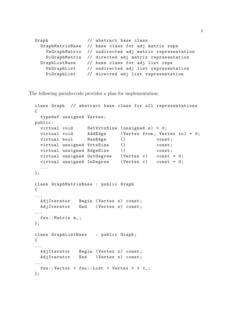
The AdjIterator type needs to be defined for both matrix and list representations.This is a forward iterator traversing the collection of vertices adjacent from v. Forthe adjacency list representation AdjIterator is a list ConstIterator. Begin can bedefined as follows:

AdjIterator GraphListBase ::Begin (Vertex x) return v_[x].Begin ();

The following implementations should completely clarify the way edges are repre-sented in all four situations:

DiGraphMatrix :: AddEdge(Vertex x, Vertex y)

M[x][y] = 1;

UnGraphMatrix :: AddEdge(Vertex x, Vertex y)

M[x][y] = 1;M[y][x] = 1;

DiGraphList :: AddEdge(Vertex x, Vertex y)

v[x]. Insert(y);

UnGraphList :: AddEdge(Vertex x, Vertex y)

v[x]. Insert(y);v[y]. Insert(x);

2 Search

One of the first things we want to do in a graph or digraph is find our way around.There are two widely used and famous processes to perform a search in a graph,both of which have been introduced and used in other contexts: depth-first andbreadth-first search. In trees, for example, preorder and postorder traversals followthe depth-first search process, and levelorder traversal follows the breadth-first pro-cess. And solutions to maze problems typically use one or the other to construct asolution path from start to goal. Trees and mazes are representable as special kindsof graphs (or digraphs), and that context provides the ultimate generality to studythese fundamental algorithms.

10

We will assume throughout the remainder of this chapter that G = (V, E) is agraph, directed or undirected, with |V | vertices and |E| edges. We also assume thatthe graph is presented to the search algorithms using the adjacency list representation.

2.1 Breadth-First Search

The Breadth-First Search [BFS] process begins at a vertex of G and explores the graphfrom that vertex. At any stage in the search, BFS considers all vertices adjacent fromthe current vertex before proceeding deeper into the graph.

Breadth First Search (v)Uses: double ended control queue conQ

vector of bool visited

for each i, visited[i] = false;conQ.PushBack(v);visited[v] = true;// PreProcess (0,v);while (!conQ.Empty ())

f = conQ.Front ();if (n = unvisited adjacent from f)

conQ.PushBack(n); // PushFIFOvisited[n] = true;// PreProcess(f,n);

else

conQ.PopFront ();// PostProcess(f);

This statement of the algorithm shows the control structure only, which uses thecontrol queue and visited flags, with other activities gathered under Pre- and Post-processing of vertices and edges. The PreProcess and PostProcess calls may be mod-ified to suit the target purpose of the search. If a particular goal vertex g is sought,PostProcess can check whether n = g and return if true. It is usually also desireableto return a solution path, in which case PreProcess can record the information thatf is the predecessor of n in the search.

11

The runtime of BFS is straightforward to estimate, ignoring the cost of pre andpost processing. The aggregate runtime cost breaks down into three categories:

Total Cost = cost of initializing the visited flags

+ cost of the calls to queue push/pop operations

+ cost of finding the unvisited adjacents.

Initializing the visited flags costs Θ(|V |). There is one push and one pop operationfor each edge in the graph that is accessible from v, so that the number of queueoperations is no greater than 2|E|. The third term is dependent on the graph repre-sentation, which we assume is the adjacency list. Finding the next unvisited vertexadjacent from f requires sequential search of the adjacency list. This search is ac-complished using an adjacency iterator that pauses when the next unvisited adjacentis found. The iterator is re-started where it is paused, but never re-initialized. More-over, a given adjacency list is traversed only one time, when its vertex is at the frontof the queue. Therefore the cost of finding unvisited adjacents is the aggregate cost oftraversing all of the adjacency lists one time. The aggregate size of adjacency lists is2|E| for graphs and |E| for digraphs, but also all (reachable) vertices must be tested,so the cost of finding all of the next unvisited adjacents is O(|V | + |E|). Thereforethe runtime is bounded above by Θ(|V |) + O(|E|) + O(|V |+ |E|):

Theorem 2. The runtime of BFS is O(|V |+ |E|).

We cannot conclude the estimate is tight only because not all edges are accessiblefrom a given vertex.

As an example, performing BFS(5) on the graph G1 encounters the vertices asfollows:

adj l i s t rep Graph G1 BFS : : conQ

−−−−−−−−−−−− −−−−−−−− <−−−−−−−−v [ 0 ] : 1 , 3 nu l l . . .

v [ 1 ] : 0 0 −−− 1 2 −−− 6 −−− 7 5 6 3 9

v [ 2 ] : 5 , 6 | | | 5 2 6 3 9 7

v [ 3 ] : 0 , 4 | | | 5 2 4 3 9 7

v [ 4 ] : 3 , 5 3 −−− 4 −−− 5 −−− 8 −−− 9 5 2 4 8 3 9 7 0

v [ 5 ] : 2 , 4 , 8 2 4 8 9 7 0

v [ 6 ] : 2 , 7 2 4 8 6 7 0

v [ 7 ] : 6 , 9 4 8 6 0

v [ 8 ] : 5 , 9 4 8 6 3 0 1

v [ 9 ] : 7 , 8 8 6 3 1

8 6 3 9 nu l l

. . .

Vertex d i s cove ry order : 5 2 4 8 6 3 9 7 0 1

grouped by d i s t ance : [ ( 5 ) (2 4 8) (6 3 9) (7 0) (1 ) ]

12

2.2 Depth-First Search

Like BFS, the Depth-First Search [DFS] process also begins at a vertex of G andexplores the graph from that vertex. In contrast to BFS, which considers all adjacentvertices before proceeding deeper into the graph, DFS follows as deep as possible intothe graph before backtacking to an unexplored possibility.

Depth First Search (v)Uses: double ended control queue conQ

vector of bool visited

for each i, visited[i] = false;conQ.PushFront(v);visited[v] = true;// PreProcess (0,v);while (!conQ.Empty ())

f = conQ.Front ();if (n = unvisited adjacent from f)

conQ.PushFront(n); // PushLIFOvisited[n] = true;// PreProcess(f,n);

else

conQ.PopFront ();// PostProcess(f);

It is remarkable that the only difference between DFS and BFS is in the way unvisitedadjacents are place on the control queue conQ. In DFS, conQ has LIFO behavior,functioning as a control stack. In BFS, conQ has FIFO behavior, functioning as acontrol queue. The effect is that in DFS, the front of conQ is the previously pushedunvisited adjacent vertex, whereas in BFS, the front of conQ remains the same afterthe unvisited adjacent vertex has been pushed.

Theorem 3. The runtime of DFS is O(|V |+ |E|).

The argument is a repeat of that for Theorem 2. Again we cannot conclude theestimate is tight only because not all edges are accessible from a given vertex.

13

Continuing with the example G1, here is a trace of DFS(5). (The orientation inthe way we show conQueue is reversed for DFS.)

adj l i s t rep Graph G1 DFS : : conQ

−−−−−−−−−−−− −−−−−−−− −−−−−−−−>

v [ 0 ] : 1 , 3 nu l l . . .

v [ 1 ] : 0 0 −−− 1 2 −−− 6 −−− 7 5 5

v [ 2 ] : 5 , 6 | | | 5 2 5 4

v [ 3 ] : 0 , 4 | | | 5 2 6 5 4 3

v [ 4 ] : 3 , 5 3 −−− 4 −−− 5 −−− 8 −−− 9 5 2 6 7 5 4 3 0

v [ 5 ] : 2 , 4 , 8 5 2 6 7 9 5 4 3 0 1

v [ 6 ] : 2 , 7 5 2 6 7 9 8 5 4 3 0

v [ 7 ] : 6 , 9 5 2 6 7 9 5 4 3

v [ 8 ] : 5 , 9 5 2 6 7 5 4

v [ 9 ] : 7 , 8 5 2 6 5

5 2 nu l l

. . .

DFS d i s cove ry order : 5 2 6 7 9 8 4 3 0 1 ( push order ) ‘ ‘ preorder ’ ’

DFS f i n i s h i n g order : 8 9 7 6 2 1 0 3 4 5 ( pop order ) ‘ ‘ postorder ’ ’

Note that the conQ is illustrated with the front (where push/pop is occurring) to theright, the way a stack is typically illustrated.

2.3 Remarks

It is worth noting the memory use patterns for BFS and DFS. In either case, memoryuse is Θ(|V |) plus the maximum size of the set of gray vertices (those currently in thecontrol queue). In the case of BFS, the gray vertices form a “search frontier” roughlya fixed distance away from the starting vertex v, growing in diameter (and typicallysize) as it moves away from v. (See Lemma 5 of Section 4.2.) In the case of DFS,the gray vertices represent the current path from v to the most recently discoveredvertex.

Of course, the sizes of these collections are dependent on the structure of the graphbeing searched. But typically, the search frontier of BFS can be significantly largerthan the longitudinal search path of DFS. This is made quite clear when searchingfrom the root of a binary tree: the BFS frontiers are cross-sections in the tree, ap-proaching |V | in size, whereas the DFS paths are downward paths in the tree, limitedto log |V | for a complete tree.

One can think of DFS as the strategy a single person might use to find a goalin a maze, armed with a way to mark locations that have been visited. The personproceeds to an adjacent unvisited vertex as long as there is one. If at some pointthere is no unvisited adjacent vertex, the person backtracks along the marked path

14

to a vertex that has an unvisited adjacent and then proceeds. Similarly, BFS mightbe a strategy employed by a search party of many people. At each vertex, the partysplits into sub-groups, one for each unvisited adjacent, and the subgroup proceeds tothat adjacent.

This analogy illustrates two important differences between DFS and BFS: (1) BFSdiscovers a most efficient path to any goal, because the various sub-search-partiesoperate concurrently and proceed away from the starting vertex. The first party toreach the goal sounds the “found” signal. (2) BFS is more expensive in its use ofmemory, because there are multiple searches in process concurrently.

3 Survey

The information that can be extracted during one of our basic search algorithms canbe very useful. On the other hand, when one has a specific goal such as discovering apath between two vertices, there may be no need for all that information. If you needto hang a picture on a wall, you don’t need a professional assessment/survey of yourproperty, only a simple tape measure. But when you want a total evaluation, a surveyis called for. For graphs and digraphs, we have two such surveys available: breadth-first and depth-first. Breadth-first survey concentrates on distance and depth-firstsurvey concentrates on time.

3.1 Breadth-First Survey

It may be past time that we succomb to the temptation to package algorithms asclasses. We do that now for the graph surveys. Here is pseudo code for a BFSurveyclass:

class BFSurveypublic:

BFSurvey ( const Graph& g );void Search ( );void Search ( Vertex v );void Reset ( );Vector < int > distance; // distance from originVector < Vertex > parent; // for BFS treeVector < Color > color; // bookkeeping

private:const Graph& g_;Vector < bool > visited_ ;Deque < Vertex > conQ_ ;

;

15

The class contains a reference to a graph object on which the survey is performed,private data used in the algorithm control, and public variables to house three resultsof the survey - distance, parent, and color for each vertex in the graph. (Thesecould be privatized with accessors and other trimmings for data security.) These dataare instantiated by the survey and have the following interpretation when the surveyis completed:

code math englishdistance[x] d(x) the number of edges travelled to get from v to x

parent[x] p(x) the vertex from which x was discoveredcolor[x] x.color either black or white, depending on whether x was reachable from v

During the course of Search, when a vertex is pushed onto the control queue in FIFOorder, it is colored gray and assigned distance one more than its parent at the frontof the queue. The vertex is colored black when popped from the queue. At any giventime during Search, the gray vertices are precisely those in the FIFO control queue.

The 1-argument constructor initializes the Graph reference and sets all the variousdata to the initial/reset state:

BFSurvey :: BFSurvey (const Graph& g): distance(g.vSize , g.eSize + 1), parent(g.vSize , null),

color(g.vSize , white), visited_(g.vSize , false),g_(g)

The Search(v) method is essentially BFSearch(v) with the pre- and post-processingfunctions defined to maintain the survey data. However, the visited flags and parentinformation are not automatically unset at the start, so that the method can becalled more than once to continue the survey in any parts of the graph that were notreachable from v.

void BFSurvey :: Search( Vertex v )

conQ_.Push(v);visited_[v] = true;distance[v] = 0;color[v] = grey;while (!conQ_.Empty ())

f = conQ_.Front ();if (n = unvisited adjacent from f in g_)

16

conQ_.PushBack(n); // PushFIFOvisited_[n] = true;distance[n] = distance[f] + 1;parent[n] = f;color[n] = grey;

else

conQ_.PopFront ();color[f] = black;

The no-argument Search method repeatedly calls Search(v), thus ensuring that thesurvey considers the entire graph. Often there are relatively few vertices not reachedon the first call, but nevertheless Search() perseveres until every vertex has beendiscovered.

void BFSurvey :: Search ()

Reset ();for (each vertex v of g_)

if (color[v] == white) Search(v);

void BFSurvey :: Reset()

for (each vertex v of g_)

visited_[v] = 0;distance[v] = g_.eSize + 1; // impossibly largeparent[v] = null;color[v] = white;

We have shown in Theorem 2 of Section 2.1 that BFSearch(v) has runtime O(|V |+|E|), and this bound carries over to BFSurvey::Search(). Note that BFSurvey::Search()touches every edge and vertex in the graph. Therefore we can apply Factoid 6 in Sec-tion 1.3.3 to conclude that the bound is tight:

Theorem 4. BFSurvey::Search() has runtime Θ(|V |+ |E|).

17

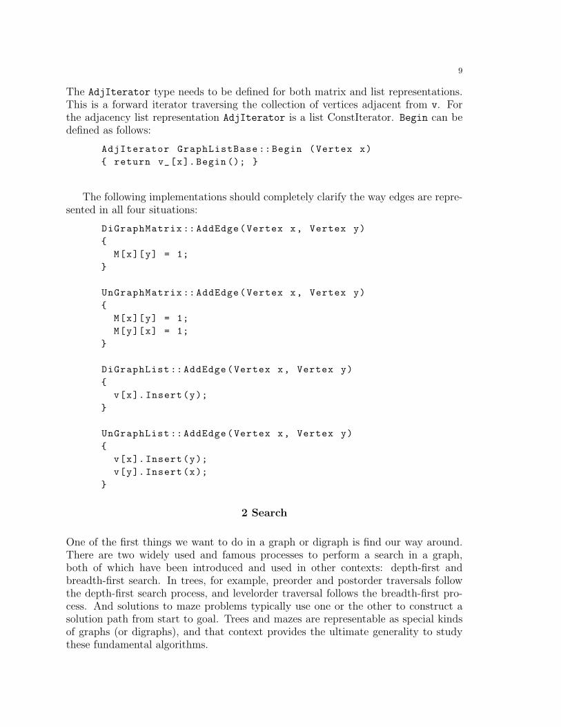
3.2 Depth-First Survey

The similarities between depth- and breadth-first search/survey algorithms are farmore numerous than the differences. Yet the differences are critical to understandingand using the two. So as tedious as it may be, it is important to concentrate byfinding the differences and understanding their consequences. Here is pseudo code fora DFSurvey class:

class DFSurveypublic:

DFSurvey ( const Graph& g );void Search ( );void Search ( Vertex v );void Reset ( );Vector < unsigned > dtime; // discovery timeVector < unsigned > ftime; // finishing timeVector < Vertex > parent; // for DFS treeVector < Color > color; // various uses

private:unsigned time_;const Graph& g_;Vector < bool > visited_ ;Deque < Vertex > conQ_ ;

;

The class structure is identical to that of BFSurvey, with these exceptions:

(1) The two DFSurvey::Search algorithms use DFS [LIFO] rather than BFS [FIFO]

(2) DFSurvey maintains global time used to time-stamp discovery time and fin-ishing time for each vertex, rather than the distance data of BFSurvey.

These time, parent, and color data are instantiated by the survey and have the fol-lowing interpretation when the survey is completed:

code math englishdtime[x] td(x) discovery time = time x is first discoveredftime[x] tf (x) finishing time = time x is released from further investigationparent[x] p(x) the vertex from which x was discoveredcolor[x] x.color black or white, depending on whether x was reachable from v

18

The 1-argument constructor initializes the Graph reference and sets all the variousdata to the initial/reset state.

During the course of Search, vertices are colored gray at discovery time andpushed onto the control queue in LIFO order, and colored black at finishing timeand popped from the queue. At any given time during Search, the gray vertices areprecisely those in the LIFO control queue.

The Search(v) method is DFSearch(v) with the pre- and post-processing functionsdefined to maintain the survey data. Note however that the visited flags are notautomatically unset at the start, so that the method can be called more than onceto continue the survey in any parts of the graph that were not reachable from v.Global time is incremented immediately after each use, which ensures that no twotime stamps are the same.

void DFSurvey :: Search( Vertex v )

dtime[v] = time_ ++;conQ_.Push(v);visited_[v] = true;color[v] = grey;while (!conQ_.Empty ())

f = conQ_.Front ();if (n = unvisited adjacent from f in g_)

dtime[n] = time_ ++;conQ_.PushFront(n); // PushLIFOvisited_[n] = true;parent[n] = f;color[n] = grey;

else

conQ_.PopFront ();color[f] = black;ftime[f] = time_ ++;

The no-argument Search method repeatedly calls Search(v), thus ensuring that thesurvey considers the entire graph.

19

void DFSurvey :: Search ()

Reset ();for (each vertex v of g_)

if (color[v] == white) Search(v);

void DFSurvey :: Reset()

for (each vertex v of g_)

visited_[v] = 0;parent[v] = null;color[v] = white;dtime[v] = 2|V|; // last time stamp is 2|V| -1ftime[v] = 2|V|;time_ = 0;

The runtime of DFSurvey::Search() succombs to an argument identical to that forBFSurvey::Search():

Theorem 5. DFSurvey::Search() has runtime Θ(|V |+ |E|).

4 Interpreting and Applying Survey Data

This section is devoted to theory of BFS and DFS, including verification that theBFS tree is a minimal distance tree and two important analytical results on DFStime stamps. We begin by defining the search trees.

4.1 BFS and DFS Trees

Note that for either BFSurvey or DFSurvey, parent informationis collected duringthe course of the algorithm and stored in the vector parent[]. Assume either DFSor BFS context, and suppose we have run Search() - the complete survey.

If parent[x] 6= null, define p(x) = ∗parent[x] = the vertex from which x is discovered,and:

20

T (s) = (p(x), x)|x 6= s and x is reachable from s

V (s) = x|x is reachable from s

F = (p(x), x)|parent[x] 6= null

Lemma 1 (Tree Lemma). After XFSurvey::Search(s), (V (s), T (s)) is a tree withroot s. If G is a directed graph, the edges of T (s) are directed away from s.

Proof. First note that s is the unique vertex in T (s) with null parent pointer, byinspection of the algorithm. Also note that (p(x), x) is an edge (directed from p(x) tox) in the graph, again by inspection of the algorithm. Following the parent pointersuntil a null pointer parent[s] = null is reached defines a (directed) path in T (s) froms to x.

Now count the vertices and edges. For each vertex x other than s, (p(x), x) isan edge distinct from any other (p(y), y) because x 6= y. Therefore the edges are in1-1 correspondence with the vertices other than s. We have a connected graph with|V (s)| = |E(s)|+ 1, so it must be a tree.

We call (V (s), T (s)) the search tree generated by the survey starting at s.

Lemma 2 (Forest Lemma). After XFSurvey::Search(), (V, F ) is a forest whosetrees are all of the search trees generated during the search:

F = ∪sT (s)

where the union is over all vertices s with parent[s] = null.

Proof. By the Tree Lemma, T (s) is a tree for each starting vertex s. Suppose someedge in F connects two of these trees, say T (s1) and T (s2). The edge must necessarilybe of the form (p(x), x) for some x, where x ∈ T (s1) and p(x) ∈ T (s2). But then theparent-path from x will pass through p(x) to s2, which means that s2 should havebeen discovered by XFSurvey::Search(s1).

We call (V, F ) the search forest generated by the survey.

4.2 Interpreting BFSurvey

We have alluded to the shortest path property of BFS in previous sections. It is timeto come to full contact with a proof, and we devote most of the rest of this sectionto doing that. We follow the proof in [Cormen et al 3e]. For any pair x, y of vertices

21

in G, define the shortest-path-distance from x to y to be δ(x, y) = the length of theshortest path from x to y in G, or δ(x, y) = 1 + |E| if y is not reachable from x.

Lemma 3. Let G = (V, E) be a directed or undirected graph and x, y, z ∈ V . If y isreachable from x and z is reachable from y then

δ(x, z) ≤ δ(x, y) + δ(y, z).

Proof. First note that z is reachable from x by concatenating shortest paths from x toy and y to z. This path from x through y to z has length δ(x, y)+δ(y, z). The shortestpath from x to z can be no longer than this path. Therefore δ(x, z) ≤ δ(x, y)+δ(y, z).

Note in passing that δ(y, z) = 1 if (y, z) ∈ E.

Assumptions. For the remainder of this section, let G = (V, E) be a directed orundirected graph and suppose BFSurvey::Search(s) has been called for some startingvertex s ∈ V . Let d(x) = distance[x] for each x ∈ V .

Lemma 4. The path in T (x) from s to x has length d(x).

Proof. Use mathematical induction on d(x).

Corollary. For each vertex x, d(x) ≥ δ(s, x).

Lemma 5. If x and y are both gray vertices (i.e., in the control queue) with x coloredgray before y (i.e., x pushed before y), then d(x) ≤ d(y) ≤ d(x) + 1.

Lemma 6. If x and y are reachable from s and x is discovered before y, then d(x) ≤d(y).

Proof. Examine the code to see that when x is pushed onto the control queue,d(x) = d(p(x)) + 1 (and at that time p(x) is the front of the queue). Show bymathematical induction that d values are non-decreasing for all vertices in the queue.Because d values are never changed once a vertex is pushed, if x is pushed before ythen d(x) ≤ d(y).

Lemma 7. d(x) = δ(s, x) for all reachable x.

Proof. Suppose that the result fails. Let δ be the smallest shortest-path-distance forwhich the result fails, and let y be a vertex for which d(y) > δ(s, y) = δ. Let x bethe next-to-last vertex on a shortest path from s to y. Then δ(s, y) = 1 + δ(s, x)

22

and, because of the minimality of δ = δ(s, y), d(x) = δ(s, x). We summarize what weknow so far:

d(y) > δ(s, y) = 1 + δ(s, x) = 1 + d(x)

Now consider the three possible colors of y at the times x is at the front of the controlqueue. If y is white, then y will be pushed onto conQ while x is at the front, makingd(y) = d(x) + 1, a contradiction. If y is black, it has been popped and d(y) ≤ d(x)by Lemma 6, again a contradiction. If y is gray, then d(y) ≤ d(x) + 1 by Lemma 4,a contradiction yet again. Therefore under all possibilities our original assumption isfalse.

Putting these facts together we have:

Theorem 6 (Breadth-First Tree Theorem). Suppose BFSurvey::Search(s)has been called for the graph or digraph G = (V, E). Then

(1) For each reachable vertex x ∈ V , d(x) is the shortest-path-distance from s tox; and

(2) The breadth-first tree contains a shortest path from s to x.

4.3 Interpreting DFSurvey

The time stamps on vertices during a DFSurvey::Search() provide a way to codify theeffects of LIFO order in the control system for DFS. We have already observed thattime stamps are unique, and one stamp is used for each change of color of a vertex.Let us define td(x) = dtime[x] and tf (x) = ftime[x] for each vertex x. Inspection ofthe algorithm shows that discovery occurs before finishing:

Lemma 8. For each vertex x, td(x) < tf (x).

Therefore the interval [td(x), tf (x)] represents the time values for which x is in thecontrol LIFO, that is, the times when x has color gray. Prior to td(x), x is white, andafter tf (x), x is black.

Theorem 7 (Parenthesis Theorem). Assume G = (V, E) is a (directed orundirected) graph and that DFSurvey::Search() has been run on G. Then for twovertices x and y, exactly one of the following three conditions holds:

(1) The time intervals [td(x), tf (x)] and [td(y), tf (y)] are disjoint, and x and ybelong to different trees in the DFS forest.

(2) [td(x), tf (x)] is a subset of [td(y), tf (y)], and x is a descendant of y in the forest.(3) [td(x), tf (x)] is a superset of [td(y), tf (y)], and x is an ancester of y in the

forest.

23

Proof. First suppose x and y belong to different trees in the forest. Then x is discov-ered during one call Search(v) and y is discovered during a different call Search(w)where v 6= w. Then x is colored gray and then black during Search(v), and y iscolored gray and then black during Search(w). Clearly these two processes do notoverlap in time, and condition (1) holds.

Suppose on the other hand that x and y are in the same tree in the search forest.Without loss of generality we assume y is a descendant of x. Then, by inspection ofthe algorithm, x must be colored gray before y. Hence, td(x) < td(y). But due tothe LIFO order of processing, this means that y is colored black before x. Thereforetf (y) < tf (x). That is, [td(y), tf (y)] is a subset of [td(x), tf (x)], and condition (3)holds. A symmetric argument completes the proof.

Theorem 8 (White Path Theorem). In a depth-first forest of a directed orundirected graph G = (V, E), vertex y is a descendant of vertex x iff at the discoverytime td(x) there is a path from x to y consisting entirely of white vertices.

Proof. First note that discovery times td(x) = dtime[x] are stamped prior to anyprocessing of x in the DFSurvey::Search algorithm.

First suppose z is a descendant of x. If z = x then x is a white path. If z 6= xthen td(x) < td(z) by the Parenthesis Theorem, so z is white at time td(x). Applyingthe observation to any z in the DFS tree path from x to y shows that the DFS treepath from x to y consists of white vertices.

Conversely, suppose at time td(x) there is a path from x to y consisting entirely ofwhite vertices. If some vertex in this path is not a descendant of x, let v be the oneclosest to x with this property. Then the predecessor u on the path is a descendantof x. At time td(u), v is white and an unvisited adjacent of u, so v will be discoveredand p(v) = u. That is, v is a descendant of u, and hence of x, contradicting theassumption that v is not a descendant of x. Therefore every vertex on the white pathis a descendant of x.

4.4 Classification of Edges

The surveys can be used to classify edges of a graph or directed graph. We will useDFSSurvey for this purpose. Given an edge, there are four possibilities: (1) it isin the DFS Forest; it goes from x to another vertex in the same tree, either (2) anancester or (3) a descendant; or (4) it goes to a vertex that is neither ancester nordescendant, whether in the same or a different tree.

24

1. Tree edges are edges in the depth-first forest.2. Back edges are edges (x, y) connecting a vertex x in the DFS forest to an ancester

y in the same tree of the forest.3. Forward edges are edges (x, y) connecting a vertex x in the DFS forest to a

descendant y in the same tree of the forest.4. Cross edges are any other edges. These might go to another vertex in the same

tree or a vertex in a different tree.

For an undirected graph, this classification is based on the first encounter of the edgein the DFSurvey.

Note these observations relating the color of the terminal vertex of an edge to theedge classification. Suppose e = (x, y) is an edge of G, and consider the moment in(algorithm) time when e is explored. Then:

1. If y is white then e is a tree edge.2. If y is gray then e is a back edge.3. If y is black then e is a forward or cross edge.

Theorem 9. In a depth-first survey of an undirected graph G, every edge is eithera tree edge or a back edge.

Proof. Let e = (x, y) be an edge of G. Since G is undirected, e = (y, x) as well, sowe can assume that x is discovered before y. At time td(x), y is white. Suppose e isfirst explored from x. Then y is white at the time, and hence e becomes a tree edge.If e is first explored from y, then x is gray at the time, and e is a back edge.

Theorem 10. A directed graph D contains no directed cycles iff a depth-first searchof D yields no back edges.

Proof. If DFS produces a back edge (x, y), adding that edge to the DFS tree pathfrom x to y creates a cycle.

If D has a (directed) cycle C, let y be the first vertex discovered in C, and let(x, y) be the preceding edge in C. At time td(y), the vertices of C form a white pathfrom y to x. By the white path theorem, x is a descendant of y, so (x, y) is a backedge.

25

5 Spinoffs from BFS and DFS

If theorems have corollaries, do algorithms have cororithms? Maybe, but that isdifficult to speak. “Spinoff” is very informal term meaning an extra outcome orsimple modification of the algorithm that requires little or no extra verification oranaylsis.

5.1 Components of a Graph

Suppose G = (V, E) is an undirected graph. G is called connected iff for every pairx, y ∈ V of vertices there is a path in G from x to y. A component of G is a graph Csuch that

(1) C is a subgraph of G,(2) C is connected, and(3) C is maximal with respect to (1) and (2)

The technology developed in Section 4.3 shows that the following instantiation ofthe DFS algorithm produces a vector component<unsigned> such that component[x]is the component containing x for each vertex x of G. All that is needed is todeclare the components vector and define PostProcess and make a small adjustmentto DFSurvey::Search():

void DFSurvey :: Search ()

unsigned components = 0;for (each vertex v of g_)

if (color[v] == white)

components +=1;Search(v);

PostProcess(f)

component[f] = components;

Recall that we know the DFS forest is a collection of trees, each tree generated by acall to Search(v). The DFS trees are in 1-1 correspondence to the components of G.

26

The algorithm above counts the components and assigns each vertex its componentnumber as it is processed.

This is an algorithm that runs in time Θ(|V |+ |E|) and computes a vector that,subsequently, looks up the component of any vertex in constant time. The algorithmdoesn’t need vertex color (equate color white with unvisited), only the minimumcontrol structure variables.

5.2 Topological Sort

A directed graph is acyclic if it has no (directed) cycles. A directed acyclic graph iscalled a DAG for short. DAGs occur naturally in various places, such as:

vertices directed edgecells in a spreadsheet dependancy from another celltargets in a makefile dependency on another targetcourses in a curriculum course pre-requisit

In these and other models, it is important to know what order to consider the vertices.For example, courses need to be taken respecting the pre-requisit structure, makeneeds to build the targets in dependency order, and a spreadsheet cell should becalculated only after the cells on which it depends have been calculated. A topologicalsort of a DAG is an ordering of its vertices in such a way that all edges go from lowerto higher vertices in the ordering.

DFS can be used to extract a topological sort from a DAG, as follows:

TopSortModifies DFSurveyUses double -ended queue outQ

Run DFSurvey(D)As a vertex x is finished , outQ.PushFront(x) // LIFO - reverses order

Then outQ [front to back] is a topological sort of D

Theorem 10 does the heavy lifting to show the correctness of TopSort.

27

Exercises

1. Conversions between directed and undirected graphs.(a) Consider an undirected graph G = (V, E) represented by either an adjacency

matrix or an adjacency list. What changes to the representations are madewhen G is converted to a directed graph? Explain.

(b) Consider a directed graph D = (V, E) represented by either an adjacencymatrix or an adjacency list. What changes to the representations are madewhen D is converted to an undirected graph? Explain.

2. Find the appropriate places in the Graph hierarchy to re-define each of the virtualmethods named in the Graph base class, and provide the implementations.

3. The way vertices are stored in adjacency lists has an arbitrary effect on the orderin which they are processed by DFS and BFS.(a) Explain these effects.(b) How might the graph edge insertion operations be modified to enforce encoun-

tering vertices in numerical order?4. Prove: During BFSurvey::Search() on a graph G, if x and y are both gray vertices

with x colored gray before y, then d(x) ≤ d(y) ≤ d(x) + 1. (This is Lemma 5above.)

5. Describe 3 other ways to find the components of a graph (other than the algorithmin Section 5.1): (a) Directly from BFS or DFS survey data, (b) Using a BFS or DFSforest, and (c) using a traversal of the graph edge set and Partition / Union-Find.

6. Consider an alternative topological sort algorithm offered first by Donald Knuth:

TopSort2Operates on: Directed Graph D = (V,E)Uses: vector <unsigned > id indexed on vertices

FIFO queue conQdouble -ended queue outQ

for each vertex x, id[x] = inDegree(x);for each vertex x

if id[x] = 0conQ.Push(x);

While (!conQ.Empty ())

f = conQ.Front ();conQ.Pop ();for every neighbor n of f

--id[f];if (id[f] == 0)

conQ.Push(n); // front or back?

28

outQ.Push (t); // front or back?

if (outQ.Size() == |V|)

export outQ as a topological sort of D (front to back)else

export ‘‘D has a cycle ’’

(a) Show that TopSort2 produces a topological sort iff D is acyclic.(b) The two push operations were not specified as FIFO (push back) or LIFO (push

front). Which choices will ensure that TopSort2 produces the same topologicalsort as TopSort?

(c) Use aggregate analysis to derive and verify the worst case runtime for TopSort2.

Software Engineering Projects

7. Develop the graph class hierarchy as outlined in Section 1.4 above. Be sure toprovide adjacency iterators facilitating BFS and DFS implementations.

8. Implement BFSurvey and DFSurvey operating on graphs and digraphs via the APIprovided by the hierarchy above.

9. Develop two classes BFSIterator and DFSIterator that may be used by UnGraphListand DiGraphList. The goal is that these traversal loops are defined for thegraph/digraph g:

for (BFSIterator i.Initialize(g,v); !i.Finished (); ++i)

std::cout << *i;for (DFSIterator i.Initialize(g,v); !i.Finished (); ++i)

std::cout << *i;

and accomplish BFSurvey::Search(v) and DFSurvey::Search(v), respectively, andoutput the vertex number in discovery order. Of course, the traversals definedwith iterators may be stopped, or paused and restarted, in the client program.The iterators should provide access to all of the public survey information.