Graphical Models forDiscrete and Continuous Data

Rui ZhuangDepartment of Biostatistics, University of Washington

andNoah Simon

Department of Biostatistics, University of Washingtonand

Johannes LedererDepartment of Mathematics, Ruhr-University Bochum

June 18, 2019

Abstract

We introduce a general framework for undirected graphical models. It generalizesGaussian graphical models to a wide range of continuous, discrete, and combinationsof different types of data. The models in the framework, called exponential tracemodels, are amenable to estimation based on maximum likelihood. We introducea sampling-based approximation algorithm for computing the maximum likelihoodestimator, and we apply this pipeline to learn simultaneous neural activities fromspike data.

Keywords: Non-Gaussian Data, Graphical Models, Maximum Likelihood Estimation

1 Introduction

Gaussian graphical models (Drton & Maathuis 2016, Lauritzen 1996, Wainwright & Jordan

2008) describe the dependence structures in normally distributed random vectors. These

models have become increasingly popular in the sciences, because their representation of

the dependencies is lucid and can be readily estimated. For a brief overview, consider a

1

arX

iv:1

609.

0555

1v3

[m

ath.

ST]

15

Jun

2019

random vector X ∈ Rp that follows a centered normal distribution with density

fΣ(x) =1

(2π)p/2√|Σ|

e−x>Σ−1x/2 (1)

with respect to Lebesgue measure, where the population covariance Σ ∈ Rp×p is a symmetric

and positive definite matrix. Gaussian graphical models associate these densities with

a graph (V,E) that has vertex set V := {1, . . . , p} and edge set E := {(i, j) : i, j ∈

{1, . . . , p}, i 6= j,Σ−1ij 6= 0}. The graph encodes the dependence structure of X in the sense

that any two entries Xi, Xj, i 6= j, are conditionally independent given all other entries if

and only if (i, j) /∈ E. A natural and straightforward estimator of Σ−1, and thus of E, is

the inverse of the empirical covariance, which is also the maximum likelihood estimator.

Inference can then be approached via the quantiles of the normal distribution.

The problem with Gaussian graphical models is that in practice, data often violate the

normality assumption. Data can be discrete, heavy-tailed, restricted to positive values, or

deviate from normality in other ways. Graphical models for some types of non-Gaussian

data have been developed, including copula-based models (Gu et al. 2015, Liu et al. 2012,

2009, Xue & Zou 2012), score matching approach (Lin et al. 2016, Yu et al. 2019), Ising

models (Brush 1967, Lenz 1920), and multinomial extensions of the Ising models (Loh &

Wainwright 2013). However, there is no general framework that comprises different data

types including finite and infinite count data, potentially heavy-tailed continuous data,

and combinations of discrete and continuous data and at the same time, ensures a rigid

theoretical structure.

We make three main contributions in this paper:

• We formulate a general framework for undirected graphical models that both encom-

passes previously studied and new models for continuous, discrete, and combined

data types.

• We show that maximum likelihood is based on a convex and smooth optimization

function and provides consistent estimation and inference for the model parameters

in the framework.

• We establish a sampling-based approximation algorithm for computing the maximum

likelihood estimator.

2

Let us have a glance at the framework. For this, we start with the Gaussian densities (1).

Our first observation is that−x>Σ−1x/2 = −〈Σ−1, xx>/2〉tr, where 〈·, ·〉tr is the trace inner

product. This formulation looks “somewhat less revealing” (Eaton 2007, Page 125) on first

sight, but it has two conceptual advantages. First, we argue that writing the parameters

and the data as algebraic duals of each other makes their relationship more symmetric.

Second, we argue that it is a good starting point for generalizations. For this, we take the

viewpoint that the exponents in the densities are linear functions of the matrix xx>/2,

and then replace this matrix by a general matrix-valued function T of x. Our second

observation is that the fundamental quantity in the family of Gaussian graphical models

is the inverse covariance matrix Σ−1 rather than the covariance matrix Σ itself. This

suggests a reparametrization of the model using the matrix Σ−1, which is then replaced by

a general matrix M. This subtlety is important: as we will see later, the matrix M contains

all information about the dependence structure of X, while the equality of M−1 and the

covariance matrix is a mere coincidence in the Gaussian case. With these two observations

in mind, and denoting the log-normalization by γ(M), with γ(M) = log((2π)p|M−1|)/2 in

the Gaussian case, we can then generalize the densities (1) to

fM(x) = e−〈M, T (x)〉tr−γ(M)

with respect to an arbitrary σ-finite measure ν, and with M, T ∈ Rq×q a matrix-valued

parameter and data function, respectively. While additional data terms can be absorbed

in the measure ν, it is sometimes illustrative to write them explicitly. We thus consider

distributions with densities of the form

fM(x) = e−〈M, T (x)〉tr+ξ(x)−γ(M) ,

where ξ(x) depends on x only. These densities form an exponential family indexed by M

and are called exponential trace models in the following for convenience.

We recall that the well-known pairwise interaction models can also be written in expo-

nential form, but there are important differences to the above formulation. First, pairwise

interaction models and exponential trace models are not sub-classes of one another: ex-

ponential trace models are not limited to pairwise interactions, while pairwise interaction

models are not limited to canonical parameterizations. Yet, importantly, exponential trace

3

models generalize pairwise interaction models in the sense that all generic examples of

pairwise interaction models are encompassed. We also highlight that in contrast to pair-

wise interaction models, we allow for q 6= p, which helps for concise formulations of mixed

graphical models, for example. In general, we argue that the exponential trace framework

is a practical starting point for general studies of graphical models, because it comprises a

very large variety of examples and still ensures a firm theoretical structure.

We carefully specify and study the described distributions in the following sections.

Section 2 contains the proposed framework: we define the densities in Section 2.1, and we

discuss a variety of examples in Sections 2.2 and 2.3. Section 3 is focused on estimation:

we discuss the maximum likelihood estimator for the model parameters in Section 3.1, and

we introduce a numerical algorithm in Sections 3.2. Section 4 shows simulation results for

different types of data. Section 5 applies the method to neural spike data. We conclude

the paper with a discussion in Section 6. The proofs are deferred to the Appendix.

Notation

For matrices A,B ∈ Rs×t, s, t ∈ {1, 2, . . . }, we denote the trace inner product (or Frobenius

inner product) by

〈A, B〉tr := tr(A>B

)=

s∑i=1

t∑j=1

AijBij

and the corresponding norm by

||A||tr :=√〈A, A〉tr =

√√√√ s∑i=1

t∑j=1

A2ij .

We consider random vectors X = (X1, . . . , Xp)> ∈ Rp. We denote random vectors and

their realizations by upper case letters such as X and arguments of functions by lower case,

boldface letters such as x. Given a set S ⊂ {1, . . . , p}, we denote by XS ∈ R|S| the vector

that consists of the coordinates of X with indices in S, and we set X−S := XSc ∈ Rp−|S|.

Independence of two elements Xi and Xj, i 6= j, is denoted by Xi ⊥ Xj; conditional

independence of Xi and Xj given all other elements is denoted by Xi ⊥⊥ Xj|X−{i,j}.

4

2 Framework

We first discuss our framework. In Section 2.1, we formulate the densities. In Section 2.2,

we show that these densities apply to standard examples of graphical models. In Section 2.3,

we study additional examples.

2.1 Exponential Trace Models

In this section, we formulate probabilistic models for vector-valued observations that have

dependent coordinates. Specifically, we consider arbitrary (non-empty) finite or continuous

domains D ⊂ Rp and random vectors X ∈ D that have densities of the form

fM(x) := e−〈M, T (x)〉tr+ξ(x)−γ(M) (2)

with respect to some σ-finite measure ν on D. For reference, we call these models expo-

nential trace models.

We begin by specifying the different components of our model. The densities are indexed

by M ∈M, where M is a subset of

M∗ := interior{M ∈ Rq×q : γ(M) <∞} .

Unlike conventional frameworks, we do not require q = p, with the advantage of concise

formulations of mixture models, for example. In generic applications, M comprises the

dependence structure of X and determines if two coordinates Xi and Xj are positively or

negatively correlated. We will discuss these aspects in the next sections. The arguably

most important note here is that the integrability condition γ(M) < ∞ is feasible. In

particular, our framework provides natural formulations of models that avoid unreasonable

restrictions on the parameter space. It is best to see this in specific examples, so that we

defer to later.

Next, the data enters the model via a matrix-valued function

T : D → Rq×q

x 7→ T (x)

5

and a real-valued function

ξ : D → R

x 7→ ξ(x) ,

and γ(M) is the normalization defined as

γ(M) := log

∫De−〈M, T (x)〉tr+ξ(x) dν .

We finally have to impose two technical assumptions on the parameter space. Our

first assumption is that the function M 7→ fM of M to the densities with respect to the

measure ν is bijective. Sufficient conditions for this are provided in (Berk 1972, Page 199)

and (Johansen 1979, Definition 1.3); we stress, however, that the bijection is required here

only on M rather than on the full set M∗. Our second assumption is that M is convex and

that M is open with respect to an affine subspace of Rq×q. The two assumptions ensure, in

particular, that the parameter M is identifiable and has a compact and “full-dimensional”

neighborhood in an affine subspace of Rq×q. Importantly, however, the assumptions are

mild enough to allow for overparametrizations in the sense that M does not have to be

open in Rq×q; a typical example is M equal to the set of symmetric matrices, seen in

Sections 2.2 and 2.3.

The exponential family formulation equips the framework with desirable structure. In

particular, we can derive the following.

Lemma 2.1. The following two properties are satisfied.

1. The set M∗ is convex;

2. for any M ∈M∗, the coordinates of T (X) have moments of all orders with respect to

fM.

Property 1 ensures that M = M∗ satisfies the above assumption about M and Property 2

ensures concentration of the maximum likelihood estimator discussed later.

2.2 Standard Graphical Models

The goal of this section is to demonstrate that standard graphical models, such as Ising

models with binary andm-ary responses and Gaussian and non-paranormal graphical mod-

6

els, fit the exponential trace framework. In combination with the results in Section 3, this

shows in particular that standard graphical models are automatically equipped with more

structure than suggested by common pairwise interaction formulations.

For the standard models, it is sufficient to consider q = p, Tij(x) ≡ Tij(xi, xj), and

ξ(x) =∑p

j=1 ξj(xj). Given M, we then define a graph G := (V,E), where V := {1, . . . , p}

is the vertex (or node) set and E := {(i, j) : i, j ∈ V, i 6= j,Mij 6= 0} the edge set.

Two matrices M,M′ ∈ M ⊂ Rp×p correspond to the same graph if and only if their non-

zero patterns are the same. In view of the examples below, we are particularly interested

in symmetric dependence structures, that is, we consider symmetric matrices M in what

follows. Then, also the edge set E is symmetric, that is, (i, j) ∈ E if and only if (j, i) ∈ E,

and the graph G is called undirected.

The corresponding models fM are a special case of pairwise interaction models (pairwise

Markov networks). Assuming that ν is a product measure, a density h with respect to ν is

a pairwise interaction model if it can be written in the form

h(x) =

p∏i,j=1

hij(xi, xj)

with positive functions hij. This means that the densities of pairwise interaction models

can be written as products of terms that depend on at most two coordinates.

The graph G now encodes the conditional dependence structure, as one can show by

applying the Hammersley-Clifford theorem (Besag 1974, Grimmett 1973). The theorem

implies that for a strictly positive density h(x) with respect to a product measure, two ele-

ments Xi, Xj are conditionally independent given all other coordinates if and only if we can

write h(x) = h1(x−i)h2(x−j), where h1, h2 are positive functions. For the described densi-

ties in our framework, we can write fM(x) = f 1M(x−i)f

2M(x−j) with positive functions f 1

M, f2M

if and only if Mij = 0. By the above definition of the graph associated with M, the latter

is equivalent to (i, j) /∈ E. We thus find

Xi ⊥⊥ Xj|X−{i,j} if and only if (i, j) /∈ E ,

meaning that the conditional dependence structure of X is represented by the edge set E.

The graph G also determines the unconditional dependence structure. To illustrate

this, we define E as the set of all connected components in M, that is, (i, j) ∈ E if and only

7

M =

1.2 −0.2 0 0

−0.2 1.5 0 0.1

0 0 1 0

0 0.1 0 0.5

1

2 4

3

Figure 1: Example of a matrix M (left) and the corresponding graph G (right).

The vertex set of the graph is V = {1, 2, 3, 4}, the edge set of the graph is E =

{(1, 2), (2, 1), (2, 4), (4, 2)}. The enlarged edge set is E = E ∪ {(1, 4), (4, 1)}. For example,

X1 and X4 are dependent (indicated by (1, 4) ∈ E), but they are conditionally independent

given the other elements of X (indicated by (1, 4) /∈ E).

if there is a path (i, i1), (i1, i2) . . . , (iq, j) ∈ E that connects i and j (in particular, E ⊂ E).

For pairwise densities in our framework, it is easy to check that

Xi ⊥ Xj if and only if (i, j) /∈ E .

Hence, the dependence structure of X is captured by E. We give an illustration of these

properties in Figure 1.

We can now turn to the examples.

2.2.1 Counting Measure

We first describe two cases where the base measure ν is the counting measure on {0, 1, . . . }p.

Specifically, we show that the well-known Ising and multinomial Ising models are encom-

passed by our framework.

Beyond the measure, a unifying property of the two examples is that the integrability

condition is satisfied for all matrices. In a formula, this reads

γ(M) <∞ for all M ∈ Rp×p . (3)

Since the set of all matrices in Rp×p is open, the integrability property (3) means that

M∗ = {M ∈ Rp×p} .

8

This ensures that any convex and (relatively) open set M ⊂ Rp×p meets our technical

assumptions. Importantly, we show later that the same properties are shared by exponential

trace models for Poisson data.

Ising The Ising model has a variety of applications, for example, in Statistical Mechanics

and Quantum Field Theory (Gallavotti 2013, Zuber & Itzykson 1977). Its densities are

proportional to

e∑pj=1 ajjxj+

∑j,k ajkxjxk

with ajk = akj, and the domain is x1, . . . , xp ∈ {0, 1}. As an illustration, consider a material

that consists of p molecules with one “magnetic” electron each. The binary variable xj then

corresponds to the electron’s spin (up or down in a given direction) in the jth molecule,

and the factor ajk determines whether the spins of the electrons in the jth and kth molecule

tend to align (ajk > 0 as in ferromagnetic materials) or tend to take opposite directions

(ajk < 0 as in anti-ferromagnetic materials). The Ising model is a special case of our

framework (2). Indeed, since 12 = 1 and 02 = 0, we can obtain the desired densities by

setting D = {0, 1}p, q = p, Mij = −aij, Tij(x) = xixj, and ξ ≡ 0. Since the domain is finite,

the integrability condition γ(M) <∞ is naturally satisfied for all matrices M.

Multinomial Ising The spin of spin 1/2 particles (such as the electron) can take two

values. Thus, the corresponding measurements can be represented by the domain {0, 1}

as in the Ising model discussed above. In contrast, the spin of spin s particles with s ∈

{1, 3/2, . . . } (such as W and Z vector bosons and composite particles) can take 2s + 1

values, which can not be represented by binaries directly. Therefore, the multinomial Ising

model, which extends the Ising model to multinomial domains, is of considerable interest

in quantum physics. For similar reasons, multinomial Ising models are of interest in other

fields, see (Diesner & Carley 2005) for an example in sociology.

We now show that also the multinomial Ising model is a special case of our framework.

For this, we encode the data in an enlarged binary vector. We first denote the original

multinomial data by Y ∈ {0, . . . ,m−1}l. This could correspond to l spin (m−1)/2 particles.

We then represent the data with an enlarged binary vector X ∈ {0, 1}p, p = l · (m− 1), by

9

setting

Xi = 1l{Yj = i− (m− 1)b i− 1

m− 1c, j = d i

m− 1e}∈ {0, 1} .

Each coordinate of the original data (for example, each spin) is now represented by m− 1

binary variables. We can use the same model as above, except for imposing the additional

requirement Mij = 0 if d im−1e = d j

m−1e to avoid self-interactions. These settings yield the

standard extension of the Ising model to multinomial data, cf. (Loh & Wainwright 2013).

In particular, for m = 2, we recover the Ising model above. Again, since the domain is

finite, the integrability condition γ(M) <∞ is naturally satisfied for all matrices M.

2.2.2 Continuous Measure

We now consider two examples in which the base measure ν is the Lebesgue measure on Rp.

Specifically, we show that Gaussian and non-paranormal graphical models are encompassed

by our framework.

We show that the integrability condition is satisfied for all matrices that are positive

definite. In a formula, this reads

γ(M) <∞ for all positive definite M ∈ Rp×p . (4)

Since the set of all positive definite matrices in Rp×p is open, this means that

M∗ ⊃ {M ∈ Rp×p : M positive definite} .

One can thus take any convex and (relatively) open set of positive definite matrices as

parameter space M. Later, we will show that very similar models can also be formulated

for exponential data, for example.

Gaussian The most popular examples are Gaussian graphical models (Lauritzen 1996).

For centered data (which can be assumed without loss of generality), these models cor-

respond to random vectors X ∼ Np(0,Σ), where Σ (and thus also Σ−1) is a symmetric,

positive definite matrix. We can generate these models in our framework (2) by setting

D = Rp, q = p, M = Σ−1, Tij(x) = xixj/2, and ξ ≡ 0.

Gaussian graphical models are well-studied and are also the starting point for our

contribution. It is thus especially important to disentangle general properties of graphical

10

models in our framework from peculiarities of the Gaussian case. First, the correspondence

of the conditional independence structure and the non-zero pattern of the inverse covariance

matrix is specific to the Gaussian case. This has already been pointed out in (Loh &

Wainwright 2013), where relationships between the dependence structure and the inverse

covariance matrix in Ising models and other exponential families with additional interaction

terms are studied. However, instead of concentrating on possible connections, we argue

that it is important to distinguish clearly between the two concepts. In our framework, the

(conditional) dependencies are completely captured by the matrix M. It is thus reasonable

to consider M the fundamental quantity. Instead, the equality of M−1 and EM[XX>] is

specific to the Gaussian case, and the (generalized) covariances EM[XX>] (2EMT (X)) and

their inverse should be viewed only as a characteristic of the model. Second, the type of

the node conditionals can change once dependencies are introduced. In the Gaussian case,

the node conditionals are normal irrespective of M. In most other cases, however, the types

of node conditionals cannot be the same in the dependent and independent case - unless

additional assumptions are introduced. We will discuss this in the later examples below.

Non-paranormal Well-known generalizations of Gaussian graphical models are non-

paranormal graphical models (Liu et al. 2009). These models correspond to vectors X such

that

(g1(X1), . . . , gp(Xp))> ∼ Np(0,Σ) for real-valued, monotone, and differentiable functions

g1, . . . , gp and symmetric, positive definite matrix Σ. These models can be generated

in our framework by setting D = Rp, q = p, M = Σ−1, Tij(x) = gi(xi)gj(xj)/2, and

ξ(x) =∑p

j=1 log |g′j(xj)|, cf. (Liu et al. 2009, Equation (2)). The normalization constant is

(irrespective of symmetry) γ(M) = log((2π)p|M−1|)/2 < ∞ both in the Gaussian and the

non-paranormal case, so that in both cases, property (4) is satisfied.

2.3 Non-standard Examples

The idea that Ising models as well as other standard graphical models can be written as

exponential families is not new (Wainwright & Jordan 2008, Chapter 3.3). However, we

argue that the details of the notions and formulations are essential, especially when it

11

comes to establishing models for data that are not covered by standard graphical models.

We will outline this in the following. We first discuss Poisson and exponential distributions.

In particular, we establish thorough proofs for the integrability of the square-root models

in (Inouye et al. 2016) and introduce extensions that show that the square-root is just one

out of many possible operations for the interaction terms and that a variety of distributions

besides Poisson can be handled.

Poisson A main objective in systems biology is the inference of microbial interactions.

The corresponding data is multivariate count data with infinite range (Faust et al. 2012).

Other fields where such data is prevalent include particle physics (radioactive decay of

particles) and criminalistics (number of crimes and arrests). However, copula-based ap-

proaches to infinite count data inflict severe identifiability issues (Genest & Nešlehová

2007), while standard extensions of the independent case lead to integrability issues, see

below. Multivariate Poisson data has thus obtained considerable attention in the recent

Machine Learning literature (Inouye et al. 2016, 2015, Yang et al. 2015, 2013), but much

less in statistics.

We show in the following that within framework (2), one can solve the problems asso-

ciated with the standard approaches while preserving the Poisson flavor of the individual

coordinates, especially in the limit of small interactions. For this, we use our framework

with the specifications D = {0, 1, . . . }p, q = p, ξ(x) = −∑p

j=1 log(xj!), and functions T

that satisfy Tii(x) = Tii(xi) = xi and Tij(x) = Tij(xi, xj) ≤ c(xi + xj) for some c ∈ (0,∞).

We note that the case Tij(x) =√xixj has been introduced in the Machine Learning litera-

ture (Inouye et al. 2016), but the technical aspects of this case have not been studied, and

the general setting has not been formulated altogether.

Most importantly, we need to show property (3). To this end, we have to verify that

for all matrices M ∈ Rp×p

∞∑x1,...,xp=0

e−∑j Mjjxj−

∑i,j:i6=j MijTij(xi,xj)∏j xj!

<∞ .

Since −MijTij(xi, xj) ≤ cxi + cxj, where c := cmaxi,j |Mij|, a sufficient condition is∞∑

x1,...,xp=0

e−∑j(Mjj−2pc)xj∏j xj!

<∞ .

12

Hence, defining C(M, j) := e−(Mjj−2pc) ∈ (0,∞), j ∈ {1, . . . , p}, the integrability condition

is implied for any M by the fact∞∑

x1,...,xp=0

p∏j=1

C(M, j)xj

xj!=

p∏j=1

eC(M,j) <∞ .

This proves property (3).

In contrast, the corresponding integrability conditions in standard approaches to this

data type inflict severe restrictions on the parameter space. To see this, recall that the

joint density of p independent Poisson random variables with parameters a1, . . . , ap > 0 is

proportional to

exp( p∑j=1

log(aj)xj −p∑j=1

log(xj!)).

The standard approach to include interactions is to add terms of the form aijxixj. This

yields densities proportional to

exp

(p∑j=1

log(aj)xj +∑i 6=j

aijxixj −p∑j=1

log(xj!)

). (5)

The dominating terms in this expression are the interaction terms aijxixj. Using Stirling’s

approximation, we find that x2/ log(x!)→∞ for x→∞, showing that the density cannot

be normalized unless aij ≤ 0 for all i, j. This means that the standard approach excludes

positive interactions between the nodes.

Let us finally look at the node conditionals for a specific T . We choose Tij(x) =√xixj

for simplicity. The node conditionals become

fM(xj|x−j) ∼ e−Mjjxj−log(xj !)LInt,

where

LInt = e−√xj

∑k∈N (j)(Mjk+Mkj)

√xk .

The off-diagonal terms in M model the interactions of j with the other nodes. If the

factors Mjk are small, LInt ≈ 1, and thus, the node j approximately follows a Poisson

distribution with parameter e−Mjj . In particular, if M is diagonal, the nodes are independent

Poisson distributed random variables.

13

In comparison, the standard approach represented by Display (5) results in exact Pois-

son node conditionals for any non-positive correlations. Conversely, it has been shown

in (Chen et al. 2015, Proposition 1 and Lemma 1) that one can find a distribution with

Poisson (or exponential) node conditionals only if all interactions are non-positive. Thus,

an unavoidable price for “pure” node conditionals is a strong, in practice typically unrealis-

tic assumption on the parameter space. Our framework avoids this assumption and is still

close to the exact Poisson (exponential) distributions if the interactions are small.

Exponential The exponential case is the counterpart of the Poisson case discussed above.

In particular, the standard approach to correlated exponential data is confronted with the

same integrability issues as above, while approaches via framework (2) easily satisfy the

integrability conditions.

To model exponential data, we consider D = [0,∞)p, q = p, and ξ ≡ 0. Again a number

of transformations T would have the desired properties; however, to avoid digression, we

only consider the square-root transformations Tij(x) =√xixj that correspond to (Inouye

et al. 2016); generalization are possible along the same lines as in the Poisson case. We

can now check the integrability condition (4). Denoting the smallest `2-eigenvalue of M by

κ(M) > 0, we find

eγ(M) =

∫ ∞0

· · ·∫ ∞

0

e−∑pi,j=1 Mij

√xixj dx1 . . . dxp

≤∫ ∞

0

· · ·∫ ∞

0

e−κ(M)||x||1 dx1 . . . dxp

=(∫ ∞

0

e−κ(M)xdx)p

=κ(M)−p <∞ .

Hence, γ(M) <∞ for all positive definite matrices M.

In contrast, adding linear interaction terms to the independent joint density forbids

positive correlations. One can check this similarly as in the Poisson case above.

The node conditionals finally become

fM(xj|x−j) ∼ e−MjjxjLInt ,

14

where

LInt = e−√xj

∑k∈N (j)(Mjk+Mkj)

√xk .

The off-diagonal terms in M model the interactions of j with the other nodes. If the

factors Mjk are small, LInt ≈ 1, and thus, node j approximately follows an exponential

distribution with parameter Mjj. In particular, if M is diagonal, all node conditionals

follow independent exponential distributions.

Composite Models As an example for composite models, let us consider data with Pois-

son and exponential elements. Note first that the conditions on the set of matrices M are

different in the discrete examples and the continuous examples: In the discrete examples,

we have shown γ(M) <∞ for any matrix M. In the continuous examples, we have shown

γ(M) <∞ under the additional assumption that M is positive definite. In the case of com-

posite models, one can interpolate the conditions. However, for the sake of simplicity, we in-

stead assume that the matrices M are positive definite. We then consider p1, p2 ∈ {1, 2, . . . },

p1 +p2 = p, D = {0, 1, . . . }p1×[0,∞)p2 , M ⊂ {M ∈ Rp×p : M symmetric, positive definite},

M open and convex, and ξ(x) = −∑p1

j=1 log(xj!). Hence, the first p1 elements of the ran-

dom vector X are discrete, while the other p2 elements are continuous. Using again the

square-root transformation, the Poisson-type node conditionals for j ∈ {1, . . . , p1} are

fM(xj|x−j) ∼ e−Mjjxj−log(xj !)LInt ,

where

LInt = e−√xj

∑k∈N (j)(Mjk+Mkj)

√xk .

The exponential-type node conditionals for j ∈ {p1 +1, . . . , p1 +p2} have the corresponding

form. The expressions highlight that the densities can include interactions between the

discrete and continuous elements of X, while the Poisson/exponential-flavors of the nodes

are still preserved.

To show that γ(M) <∞, we proceed similarly as in the examples above. More precisely,

15

denoting the smallest `2-eigenvalue of M by κ(M) > 0, we find

eγ(M) =∞∑

x1,...,xp1=0

∫ ∞0

· · ·∫ ∞

0

e−∑pi,j=1 Mij

√xixj∏p1

j=1 xj!dxp1+1 . . . dxp

≤∞∑

x1,...,xp1=0

∫ ∞0

· · ·∫ ∞

0

e−κ(M)||x||1∏p1j=1 xj!

dxp1+1 . . . dxp

=∞∑

x1,...,xp1=0

e−κ(M) (x1+···+xp1 )∏p1j=1 xj!

×∫ ∞

0

· · ·∫ ∞

0

e−κ(M) (xp1+1+···+xp2 ) dxp1+1 . . . dxp

=(ee−κ(M)

)p1(∫ ∞0

e−κ(M)xdx)p2

<∞ .

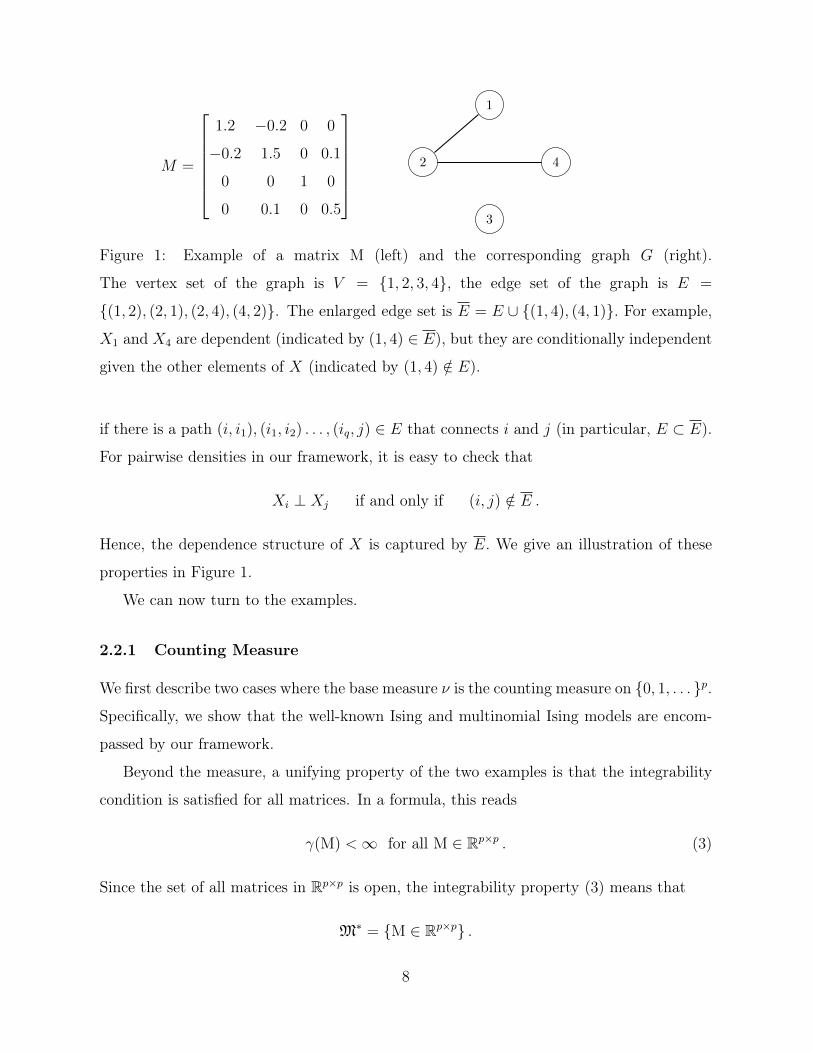
Laplace and Beyond There is much room for our creativity in constructing models. For

example, we can readily establish models for Laplace (double-exponential) data by inserting

absolute values throughout, for example, Tij(x) =√|xixj|. Indeed, again denoting the

smallest `2-eigenvalue of M by κ(M) > 0, we find

eγ(M) =

∫ ∞−∞· · ·∫ ∞−∞

e−∑pi,j=1 Mij

√|xixj | dx1 . . . dxp

≤∫ ∞−∞· · ·∫ ∞−∞

e−κ(M)||x||1 dx1 . . . dxp

=(

2

∫ ∞0

e−κ(M)xdx)p

= (2/κ(M))p <∞ .

Hence, γ(M) <∞ for all positive definite matrices M. In general, the essentially only limit

is that to ensure integrability, the interaction terms have to be of “smaller order” than the

terms that correspond to the independent case.

3 Estimation

We now turn to estimation based on maximum likelihood. In Section 3.1, we show that

maximum likelihood estimation has desirable properties in our framework. In Section 3.2,

we propose a sampling-based approximation algorithm for computing the maximum likeli-

hood estimator.

16

3.1 Maximum Likelihood Estimation

We study maximum likelihood estimation in our framework. For this, we assume we are

given n i.i.d. data samples X1, . . . , Xn from a distribution of the form (2). Also, we assume

we are given the model specifications D, ν, T, ξ and the parameter space M; that is, we

assume that the model class is known. In contrast, the correct model parameters specified

in the matrix M are unknown. Our goal is to estimate M from the data.

As a toy example, consider data on p different populations of freshwater fish in n similar

lakes. More specifically, consider vector-valued observations X1, . . . , Xn ∈ {0, 1, . . . }p,

where (X i)j is the number of fish of type j in lake i. We want to use these data to uncover

the relationships among the different populations. A model suited for this task is the

Poisson model discussed earlier. For example, we might set D = {0, 1, . . . }p, q = p, {M ∈

Rp×p : M symmetric}, Tij(x) =√xixj, and ξ(x) = −

∑pj=1 log(xi!) . The relationships

among the fish populations are then encoded in M, which then needs to be estimated from

the observations.

Before heading on, we add some convenient notation. We summarize the data in X :=

(X1, . . . , Xn) and denote the corresponding function argument by x := (x1, . . . ,xn) for

x1, . . . ,xn ∈ D. The generalized Gram matrix is denoted by

T (x) :=1

n

n∑i=1

T (xi) .

The negative joint log-likelihood function −`M for n i.i.d random vectors corresponding to

the model (2) is finally given by

−`M(x) = n〈M, T (x)〉tr −n∑i=1

ξ(xi) + nγ(M) .

We can now state the maximum likelihood estimator and its properties. For further

reference, we first state the essence of the previous discussion in the following lemma.

Lemma 3.1 (Log-likelihood). Given any M ∈ M∗, the negative joint log-likelihood func-

tion −`M of n i.i.d. random vectors distributed according to fM in (2) can be expressed

by

−`M(x) = n〈M, T (x)〉tr + nγ(M) + c ,

where c ∈ R does not depend on M.

17

Motivated by Lemma 3.1, we introduce the maximum likelihood estimator of M by

M := argminM∈M

{− `M(X)

}= argmin

M∈M

{〈M, T (X)〉tr + γ(M)

}. (6)

The estimator exists in all generic examples. More generally, under our assumption that

M ∈M ⊂M∗ and M is open and convex, and the minimizer exists for n sufficiently large,

cf. (Berk 1972). In particular, the objective function is convex, and its derivatives can be

computed explicitly.

Lemma 3.2 (Convexity). For any x ∈ Dp, the function

M∗ → R

M 7→ 〈M, T (x)〉tr + γ(M)

is convex.

Lemma 3.3 (Derivatives). For any x ∈ Dp, the function

M∗ → R

M 7→ 〈M, T (x)〉tr + γ(M)

is twice differentiable with partial derivatives

∂

∂Mij

(〈M, T (x)〉tr + γ(M)

)= T ij(x)− EMT ij(X)

and

∂

∂Mij

∂

∂Mkl

(〈M, T (x)〉tr + γ(M)

)= nEM

[(T ij(X)− EMT ij(X)

)(T kl(X)− EMT kl(X)

)]for i, j, k, l ∈ {1, . . . q}.

Convexity and the explicit derivatives are desirable for both optimization and theory. From

an optimization perspective, the two properties are valuable, because they render the ob-

jective function amenable to gradient-type minimization. From a theoretical perspective,

the two properties are valuable, because they imply that

M = argminM∈M

{EM

[〈M, T (X)〉tr + γ(M)

]},

18

showing that M is a standard M-estimator, and because they imply that M can be written

as a Z-estimator (note that M is necessarily in the interior of M) with criterion

T (X) = EMT (X) .

A simple special case is the multivariate Gaussian model. Recall that in this case, M is

the inverse of the usual population covariance matrix. Moreover, one can check that

T (x) =1

n

n∑i=1

xixi>

and M = T (X)−1. Hence, in this case, the estimator M is the inverse of the (usual) sample

covariance matrix.

Remark 3.1. The maximum likelihood estimator of M is asymptotically normal with co-

variance equal to the inverse Fisher information. In particular, consistency and asymptotic

normality of the maximum likelihood estimator can be proved following the arguments in

the classical paper (Berk 1972), see especially (Berk 1972, Theorems 4.1 and 6.1). We refer

to that paper for details.

3.2 Algorithm

The main challenge in computing the maximum likelihood estimator is the unconventional

normalization term. We address this challenge by approximating the objective function

using a sampling-based technique. In this section, we describe the corresponding algorithm.

We denote the objective function of the maximum likelihood estimator in Equation (6)

as

g(M) := 〈M, T (X)〉tr + γ(M).

The normalization term γ(M), in general, does not have a closed-form formula and, there-

fore, makes the objective function hard to compute exactly. However, we show in the

following that it can be feasibly approximated. Adding the constant term γ(M0), where

M0 is a pre-specified constant parameter matrix, to the objective function of (6) yields an

equivalent definition of the maximum likelihood estimator as

M = argminM∈M

{〈M, T (X)〉tr + γ(M)− γ(M0)

}. (7)

19

Algebraic transformation reveals

γ(M)− γ(M0) = logEM0

(e−〈M−M0, T (x)〉tr

).

The finite expectation can be approximated by an empirical mean based on some sample

set Y from the distribution fM0(x) := exp(−〈M0, T (x)〉tr + ξ(x)− γ(M0)). By the strong

law of large numbers, when the cardinality of the set Y (denoted as |Y |) goes to infinity,

the empirical mean approximates the expectation well:

log1

|Y |∑Z∈Y

e−〈M−M0, T (Z)〉tr a.s−→ logEM0

(e−〈M−M0, T (x)〉tr

).

Hence, in practice, we solve the approximate problem

M ≈ argminM∈M

{g(M)

}, (8)

where

g(M) := 〈M, T (X)〉tr + log1

|Y |∑Z∈Y

e−〈M−M0, T (Z)〉tr .

We apply gradient descent to solve the problem of (8). The gradient with respect to M is

∇g(M) = T (X)−∑

Z∈Y T (Z)e−〈M−M0, T (Z)〉tr∑Z∈Y e

−〈M−M0, T (Z)〉tr. (9)

Remark 3.2. The gradient in (9) can also be considered as an instantiation of self-

normalized importance sampling (Owen 2013). Lemma 3.3 gives the gradient of g(M) in

the form of

∇g(M) = T (X)− EMT (X) = T (X)− EMT (X) .

When EMT (X) lacks an algebraic expression and fM is inconvenient to sample from, im-

portance sampling (Owen 2013) is useful to approximate the expectation term EMT (X).

The idea of importance sampling is to draw samples from a biased distribution and obtain

the desired fM by adjusting the weights for the drawn samples. Self-normalized importance

sampling refers to the special case when weights are normalized by their sum. Equation (9)

reflects the same idea and uses the pre-specified fM0 as the biased sampling distribution.

The choice of M0 is essential for the finite-sample performance of the approximation.

Our two main considerations are: First, the sampling distribution fM0 should be straight-

forward for generating samples. Second, it should lead to balanced weights and a small

20

variance of EMT (X); if weights concentrate in just a few samples, we have effectively only

got these observations, resulting in large variability of the approximation (Owen 2013). To

incorporate the two considerations, we propose

M0 := argminM∈M

{〈M, T (X)〉tr + γ(M)

}subject to Mkl = 0, ∀k 6= l. (10)

We restrict the parameter to a diagonal matrix, by which we presume mutual independence

among all coordinates and disentangle the objective function. Hence, both the optimiz-

ing problem (10) and the task of sampling from fM0 can be handled for each coordinate

separately, and each coordinate reduces to a standard univariate exponential family dis-

tribution. Besides, M0 is the diagonal matrix closest to the actual parameter. When the

off-diagonal entries of the actual parameter matrix are small, weights of the drawn samples

are expected to be reasonable.

Algorithm 1 summarizes our computational pipeline. In the full version, which is stated

in Appendix B, a backtracking line search selects the step size adaptively and incorporates

the domain constraint as needed (for example, the positive definite requirement for the case

of continuous measures).

4 Simulation Studies

Exponential trace models apply to a large variety of multivariate data that have correlated

coordinates. The framework is especially useful for data that are discrete, heavy-tailed, or

composed of different data types. We consider the following four model-types in simula-

tions: Poisson, Exponential, Poisson-Bernoulli (a composite of Poisson and Bernoulli), and

Poisson-Gaussian (a composite of Poisson and Gaussian). Such types of models are useful

in practice but, to date, have proven challenging to characterize and estimate.

4.1 Settings

We follow the discussion of Section 2.3 and consider the square-root transformation for

non-Gaussian data as one example, that is, we set Tij(x) = ti(xi)tj(xj), where ti(xi) =√xi

for non-Gaussian coordinates and ti(xi) = xi for Gaussian coordinates.

21

Algorithm 1: Solving for the maximum likelihood estimator

// η: step size

Input : T (X), η > 0

Output: M

// Solve for M0

1 M0 ← 0p×p;

2 for i = 1, . . . , p do

3 (M0)ii ← argminm∈R

{mT ii(X) + log

∫exp

(−mTii(x) + ξ(xi)

)dxi

};

// Generate sample set Y from fM0 =∏p

i=1 f(M0)ii(xi)

4 for i = 1, . . . , p do

5 Generate 10,000 random samples from f(M0)ii(xi) for the i-th coordinate;

// Apply gradient descent with constant step size to (8)

6 k ← 0;

7 Mk ← M0;

8 repeat

9 k ← k + 1;

10 ∇g(Mk−1)← T (X)−∑Z∈Y T (Z)e−〈Mk−1−M0, T (Z)〉tr∑Z∈Y e

−〈Mk−1−M0, T (Z)〉tr;

11 Mk ← Mk−1 − η∇g(Mk−1);

12 until∣∣g(Mk)− g(Mk−1)

∣∣ < 10−4;

13 M← Mk;

22

In the following, we describe the specific graph structures for discrete data, continuous

data, and composite data of both types. The discrete data category also covers composite

data of different discrete types (for example, Poisson-Bernoulli).

Discrete Data

We consider Erdős-Rényi random graphs and generate the corresponding p× p parameter

matrix M in the following manner. Let c0 and c1 be two constants (c1 6= 0). We set

the diagonal entries to Mii = c0. For i 6= j, the off-diagonal entries are independent and

identically distributed as

Mij = Mji =

c1 with probability 1/p,

−c1 with probability 1/p,

0 with probability 1− 2/p.

(11)

The corresponding Erdős-Rényi random graph has p−1 edges in expectation, among which

half represent positive interactions and the other half negative ones.

Continuous Data

We consider again Erdős-Rényi random graphs. In addition, we generate strictly diagonally

dominant matrices with positive diagonal entries for the parameter matrix M. It can be

shown that the M’s are positive definite and satisfy the integrability condition. More

specifically, we first generate a p× p adjacency matrix with i.i.d. off-diagonal entries

Aij = Aji =

1 with probability 1/p,

−1 with probability 1/p,

0 with probability 1− 2/p,

We denote the maximum node degree by s := maxi∑

j 6=i |Aij|. Then, a positive definite M

can be generated by setting the diagonal entries to 1 and the off-diagonal entries to

Mij = Mji = 1/(s+ 0.1)Aij.

The corresponding Erdős-Rényi random graph has p−1 edges in expectation, among which

half represent positive interactions and the other half negative ones.

23

A Composite of Discrete and Continuous Data

We consider even values of p, with the first p1 = p/2 coordinates discrete, and the remaining

p2 = p/2 coordinates continuous. The parameter matrix in blockwise format is

M =

M11 M12

M>12 M22

,where M11,M22 represent the conditional dependences among p1 discrete and p2 continuous

coordinates, respectively. The remaining block M12 describes the conditional dependences

between discrete and continuous coordinates. When the continuous node conditionals follow

a Gaussian distribution, the integrability condition is satisfied for all M ∈ Rp×p such that

M22 is positive definite. Therefore, we generate M22 in the above described continuous case

to guarantee its positive definiteness while generating M11 and M12 in the above described

discrete case.

4.2 Results

We evaluate the maximum likelihood estimators in terms of edge recovery by studying

average ROC (receiver operating characteristic) curves based on thresholding maximum

likelihood estimates. Each average ROC curve is taken over 50 individual ROC curves

that correspond to 50 different Erdős-Rényi random graphs. ROC curves are combined

using horizontal-averaging via the R package ROCR (Sing et al. 2005). Since Gaussian

graphical models are currently widely used, even in cases with obvious misspecification

(eg. count data) (Zhao & Duan 2019), we compare the maximum likelihood estimators of

the exponential trace model to that of the (misspecified) Gaussian graphical model.

The graph structures are described in Section 4.1. Details regarding the data generation

approaches are deferred to Appendix C. We use n = 250 independent observations to

recover the conditional dependence of p = 20 variables. The diagonal entry is c0 = −1

and the off-diagonal entry is c1 = 0.3. We show the average ROC curves of Poisson,

Exponential, Poisson-Bernoulli, and Poisson-Gaussian in Figures 2 and 4. In addition, we

explore scenarios with diagonal entry c0 ∈ {0,−0.5,−1,−1.5,−2} and off-diagonal entry

24

(a) Poisson

Average false positive rate

True

pos

itive

rat

e

0.0 0.2 0.4 0.6 0.8 1.0

0.0

0.2

0.4

0.6

0.8

1.0

ETMGGM

(b) Exponential

Average false positive rate

True

pos

itive

rat

e

0.0 0.2 0.4 0.6 0.8 1.0

0.0

0.2

0.4

0.6

0.8

1.0

ETMGGM

Figure 2: Average ROC curves for pure data. ETM stands for the Exponential trace mode

and GGM stands for Gaussian graphical model.

c1 ∈ {0.1, 0.2, 0.3, 0.4, 0.5} : we show the differences in AUC of average ROC curves between

the exponential trace model and the Gaussian graphical model in Figures 3 and 5.

In the pure data type scenarios: The exponential trace model outperforms the Gaus-

sian graphical model substantially—the expoential trace model’s ROC curves lie entirely

above the Gaussian graphical model’s ROC curves—in the scenario of small interaction and

small sufficient statistics T (x) (see Figure 2). In addition, we look into more configurations

of Poisson type scenarios by varying c0 and c1: the performance of the sampling-based

approximation determines that of the exponential trace model (see Figure 3). When the

interaction term and sufficient statistics are small to moderate, the exponential trace model

has a larger AUC than the Gaussian graphical model. But when the interaction term and

sufficient statistics are large, for example, c0 = −2 and c1 = 0.5, the improvement is not

guaranteed. For the composite data type scenarios: The exponential trace model shows

improved performance for Poisson-Bernoulli data but not for Poisson-Gaussian data (see

Figures 4 and 5). Bernoulli data have very small sufficient statistics so that the improve-

25

●

●●

●●

−2.0 −1.5 −1.0 −0.5 0.0

−0.

15−

0.05

0.05

0.15

(a) Poisson

c0

∆ A

UC

● c1 = 0.1c1 = 0.2c1 = 0.3c1 = 0.4c1 = 0.5

●

●●

●●

0.1 0.2 0.3 0.4 0.5

−0.

15−

0.05

0.05

0.15

(b) Poisson

c1∆

AU

C

● c0 = 0c0 = −0.5c0 = −1c0 = −1.5c0 = −2

Figure 3: Differences in AUC of average ROC curve between exponential trace model and

Gaussian graphical model for Poisson data.

(a) Poisson−Bernoulli

Average false positive rate

True

pos

itive

rat

e

0.0 0.2 0.4 0.6 0.8 1.0

0.0

0.2

0.4

0.6

0.8

1.0

ETMGGM

(b) Poisson−Gaussian

Average false positive rate

True

pos

itive

rat

e

0.0 0.2 0.4 0.6 0.8 1.0

0.0

0.2

0.4

0.6

0.8

1.0

ETMGGM

Figure 4: Average ROC curves for composite data. ETM stands for the Exponential trace

mode and GGM stands for Gaussian graphical model.

26

●

●●●

●

−2.0 −1.5 −1.0 −0.5 0.0

−0.

2−

0.1

0.0

0.1

0.2

(a) Poisson−Bernoulli

c0

∆ A

UC

● c1 = 0.1c1 = 0.2c1 = 0.3c1 = 0.4c1 = 0.5

●

● ● ● ●

0.1 0.2 0.3 0.4 0.5−

0.2

−0.

10.

00.

10.

2

(b) Poisson−Bernoulli

c1

∆ A

UC

● c0 = 0c0 = −0.5c0 = −1c0 = −1.5c0 = −2

●●●

●●

−2.0 −1.5 −1.0 −0.5 0.0

−0.

2−

0.1

0.0

0.1

0.2

(c) Poisson−Gaussian

c0

∆ A

UC

● c1 = 0.1c1 = 0.2c1 = 0.3c1 = 0.4c1 = 0.5

●

●

●

●

●

0.1 0.2 0.3 0.4 0.5

−0.

2−

0.1

0.0

0.1

0.2

(d) Poisson−Gaussian

c1

∆ A

UC

● c0 = 0c0 = −0.5c0 = −1c0 = −1.5c0 = −2

Figure 5: Differences in AUC of average ROC curves between exponential trace model and

Gaussian graphical model for composite data.

27

ment in Poisson-Bernoulli data is substantial for a large range of interaction terms, but

Poisson-Gaussian data involves Gaussian coordinates, so that the performance of the expo-

nential trace model is mixed. The comparative performance is not only determined by the

performance of the approximation algorithm but also the degree to which the conditional

dependence structure resembles the zero pattern of the precision matrix.

In conclusion, the simulation study shows that: (1) the exponential trace model can

improve on the Gaussian graphical model for non-Gaussian data, especially when the suf-

ficient statistics and small interactions are small; (2) the approximation approach can

struggle when sufficient statistics and interactions are large. Based on this, we believe

that our modeling approach has substantial potential: Some of this potential is realized

by our current implementation, however some of the potential might require additional

computational insights.

5 Application to Neural Spike Data

In this section, we apply the proposed exponential trace model to neural spike data. The

temporal and spatial patterns of neural spikes capture the concurrent activity of neurons.

Understand this is essential for learning neural circuits. Neural spike data is usually formu-

lated as spike counts in a short time bin and modeled by a Poisson distribution (Theis et al.

2016). We consider a data set of multi-electrode array recordings of spike trains in mouse

retina (Demas et al. 2003) obtained from the Retinal Wave Repository (Home page for the

Retinal Wave Repository 2014). We transform the spike time data into spike counts in time

bins of 40ms following conventions in neural science (Theis et al. 2016). The short time

interval captures the instantaneous characteristics of neuron firing. The recording covers

an 800 × 800µm surface area and provides locations of each recorded unit in the form of

(x, y)-coordinates. The number of recorded units ranges from 12 to 22 in different mice.

The spike counts of each recorded unit range from 0 to 13 and roughly follow the mean-

variance relationship of a Poisson distribution. The small counts imply: (1) the exponential

trace model with square-root transformation is close to the Poisson one; (2) the proper-

ties of the data fit the scenario for which the proposed algorithm is appropriate. These

two observations render the exponential trace model with a square-root transformation

28

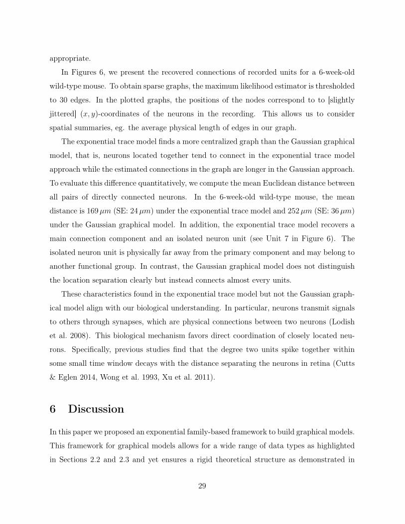
appropriate.

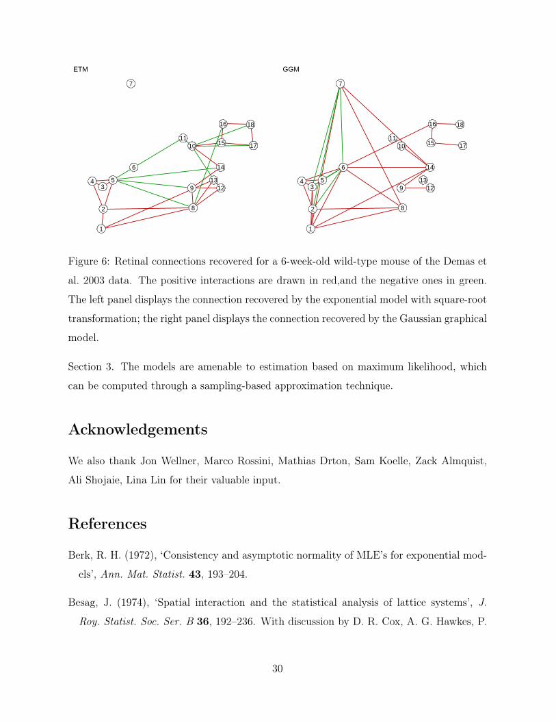
In Figures 6, we present the recovered connections of recorded units for a 6-week-old

wild-type mouse. To obtain sparse graphs, the maximum likelihood estimator is thresholded

to 30 edges. In the plotted graphs, the positions of the nodes correspond to to [slightly

jittered] (x, y)-coordinates of the neurons in the recording. This allows us to consider

spatial summaries, eg. the average physical length of edges in our graph.

The exponential trace model finds a more centralized graph than the Gaussian graphical

model, that is, neurons located together tend to connect in the exponential trace model

approach while the estimated connections in the graph are longer in the Gaussian approach.

To evaluate this difference quantitatively, we compute the mean Euclidean distance between

all pairs of directly connected neurons. In the 6-week-old wild-type mouse, the mean

distance is 169µm (SE: 24µm) under the exponential trace model and 252µm (SE: 36µm)

under the Gaussian graphical model. In addition, the exponential trace model recovers a

main connection component and an isolated neuron unit (see Unit 7 in Figure 6). The

isolated neuron unit is physically far away from the primary component and may belong to

another functional group. In contrast, the Gaussian graphical model does not distinguish

the location separation clearly but instead connects almost every units.

These characteristics found in the exponential trace model but not the Gaussian graph-

ical model align with our biological understanding. In particular, neurons transmit signals

to others through synapses, which are physical connections between two neurons (Lodish

et al. 2008). This biological mechanism favors direct coordination of closely located neu-

rons. Specifically, previous studies find that the degree two units spike together within

some small time window decays with the distance separating the neurons in retina (Cutts

& Eglen 2014, Wong et al. 1993, Xu et al. 2011).

6 Discussion

In this paper we proposed an exponential family-based framework to build graphical models.

This framework for graphical models allows for a wide range of data types as highlighted

in Sections 2.2 and 2.3 and yet ensures a rigid theoretical structure as demonstrated in

29

1

2

34 5

6

7

8

9

1011

1213

14

15

16

17

18

ETM

1

2

34 5

6

7

8

9

1011

1213

14

15

16

17

18

GGM

Figure 6: Retinal connections recovered for a 6-week-old wild-type mouse of the Demas et

al. 2003 data. The positive interactions are drawn in red,and the negative ones in green.

The left panel displays the connection recovered by the exponential model with square-root

transformation; the right panel displays the connection recovered by the Gaussian graphical

model.

Section 3. The models are amenable to estimation based on maximum likelihood, which

can be computed through a sampling-based approximation technique.

Acknowledgements

We also thank Jon Wellner, Marco Rossini, Mathias Drton, Sam Koelle, Zack Almquist,

Ali Shojaie, Lina Lin for their valuable input.

References

Berk, R. H. (1972), ‘Consistency and asymptotic normality of MLE’s for exponential mod-

els’, Ann. Mat. Statist. 43, 193–204.

Besag, J. (1974), ‘Spatial interaction and the statistical analysis of lattice systems’, J.

Roy. Statist. Soc. Ser. B 36, 192–236. With discussion by D. R. Cox, A. G. Hawkes, P.

30

Clifford, P. Whittle, K. Ord, R. Mead, J. M. Hammersley, and M. S. Bartlett and with

a reply by the author.

Brush, S. G. (1967), ‘History of the Lenz-Ising model’, Reviews of modern physics

39(4), 883.

Chen, S., Witten, D. M. & Shojaie, A. (2015), ‘Selection and estimation for mixed graphical

models’, Biometrika 102(1), 47–64.

Cutts, C. S. & Eglen, S. J. (2014), ‘Detecting pairwise correlations in spike trains: An ob-

jective comparison of methods and application to the study of retinal waves’, J. Neurosci.

34(43), 14288–14303.

Demas, J., Eglen, S. J. & Wong, R. O. (2003), ‘Developmental loss of synchronous spon-

taneous activity in the mouse retina is independent of visual experience’, J. Neurosci.

23(7), 2851–2860.

Diesner, J. & Carley, K. M. (2005), Exploration of communication networks from the enron

email corpus, in ‘SIAM International Conference on Data Mining: Workshop on Link

Analysis, Counterterrorism and Security, Newport Beach, CA’, Citeseer.

Drton, M. & Maathuis, M. H. (2016), ‘Structure learning in graphical modeling’,

arXiv:1606.02359 .

Eaton, M. L. (2007), ‘Multivariate statistics: A vector space approach’, IMS Lecture Notes

Monogr. Ser. 53.

URL: http://projecteuclid.org/euclid.lnms/1196285102

Faust, K., Sathirapongsasuti, J. F., Izard, J., Segata, N., Gevers, D., Raes, J. & Hut-

tenhower, C. (2012), ‘Microbial co-occurrence relationships in the human microbiome’,

PLOS Comput. Biol. 8(7), e1002606.

Gallavotti, G. (2013), Statistical mechanics: A short treatise, Springer Science & Business

Media.

31

Genest, C. & Nešlehová, J. (2007), ‘A primer on copulas for count data’, Astin Bull.

37(2), 475–515.

Grimmett, G. R. (1973), ‘A theorem about random fields’, Bull. London Math. Soc. 5, 81–

84.

Gu, Q., Cao, Y., Ning, Y. & Liu, H. (2015), ‘Local and global inference for high dimensional

nonparanormal graphical models’, arXiv:1502.02347 .

Home page for the Retinal Wave Repository (2014), http://www.damtp.cam.ac.uk/user/

eglen/waverepo.

Inouye, D. I., Ravikumar, P. & Dhillon, I. S. (2016), ‘Square root graphical models: Multi-

variate generalizations of univariate exponential families that permit positive dependen-

cies’, Proceedings of the International Conference on Machine Learning .

Inouye, D. I., Ravikumar, P. K. & Dhillon, I. S. (2015), Fixed-length Poisson MRF: adding

dependencies to the multinomial, in ‘NIPS’, pp. 3195–3203.

Johansen, S. (1979), Introduction to the theory of regular exponential families, Vol. 3 of

Lecture Notes, University of Copenhagen, Institute of Mathematical Statistics, Copen-

hagen.

Lauritzen, S. L. (1996), Graphical models, Vol. 17 of Oxford Statistical Science Series, The

Clarendon Press, Oxford University Press, New York. Oxford Science Publications.

Lenz, W. (1920), ‘Beiträge zum Verständnis der magnetischen Eigenschaften in festen

Körpern’, Physikalische Zeitschrift 21, 613–615.

Lin, L., Drton, M. & Shojaie, A. (2016), ‘Estimation of high-dimensional graphical models

using regularized score matching’, Electron. J. Stat. 10(1), 806.

Liu, H., Han, F., Yuan, M., Lafferty, J. & Wasserman, L. (2012), ‘High-dimensional semi-

parametric Gaussian copula graphical models’, Ann. Statist. 40(4), 2293–2326.

Liu, H., Lafferty, J. & Wasserman, L. (2009), ‘The nonparanormal: semiparametric esti-

mation of high dimensional undirected graphs’, J. Mach. Learn. Res. 10, 2295–2328.

32

Lodish, H., Darnell, J. E., Berk, A., Kaiser, C. A., Krieger, M., Scott, M. P., Bretscher,

A., Ploegh, H. & Matsudaira, P. (2008), Molecular cell biology, Macmillan.

Loh, P.-L. & Wainwright, M. J. (2013), ‘Structure estimation for discrete graphical models:

generalized covariance matrices and their inverses’, Ann. Statist. 41(6), 3022–3049.

Mahani, A. S. & Sharabiani, M. T. (2014), ‘Multivariate-from-univariate MCMC sampler:

R Package MfUSampler’, arXiv:1412.7784 .

Neal, R. M. (2003), ‘Slice sampling’, Ann. Statist. 31(3), 705–767.

Owen, A. B. (2013), Monte Carlo theory, methods and examples.

Shao, J. (2003), Mathematical statistics, Springer Texts in Statistics, second edn, Springer-

Verlag, New York.

Sing, T., Sander, O., Beerenwinkel, N. & Lengauer, T. (2005), ‘ROCR: visualizing classifier

performance in R’, Bioinformatics 21(20), 3940–3941.

Theis, L., Berens, P., Froudarakis, E., Reimer, J., Rosón, M. R., Baden, T., Euler, T.,

Tolias, A. S. & Bethge, M. (2016), ‘Benchmarking spike rate inference in population

calcium imaging’, Neuron 90(3), 471–482.

Wainwright, M. J. & Jordan, M. I. (2008), Graphical models, exponential families, and

variational inference, Vol. 1, Now Publishers Inc.

Wong, R. O., Meister, M. & Shatz, C. J. (1993), ‘Transient period of correlated bursting

activity during development of the mammalian retina’, Neuron 11(5), 923–938.

Xu, H.-p., Furman, M., Mineur, Y. S., Chen, H., King, S. L., Zenisek, D., Zhou, Z. J.,

Butts, D. A., Tian, N., Picciotto, M. R. & Crair, M. C. (2011), ‘An instructive role

for patterned spontaneous retinal activity in mouse visual map development’, Neuron

70(6), 1115–1127.

Xue, L. & Zou, H. (2012), ‘Regularized rank-based estimation of high-dimensional non-

paranormal graphical models’, Ann. Statist. 40(5), 2541–2571.

33

Yang, E., Ravikumar, P., Allen, G. I. & Liu, Z. (2015), ‘On graphical models via univariate

exponential family distributions’, J. Mach. Learn. Res. 16, 3813–3847.

Yang, E., Ravikumar, P. K., Allen, G. I. & Liu, Z. (2013), On Poisson graphical models,

in ‘NIPS’, pp. 1718–1726.

Yu, S., Drton, M. & Shojaie, A. (2019), ‘Generalized score matching for non-negative data.’,

J. Mach. Learn. Res. 20(76), 1–70.

Zhao, H. & Duan, Z.-H. (2019), ‘Cancer genetic network inference using Gaussian graphical

models’, Bioinform. Biol. Insights 13, 1–9.

Zuber, J.-B. & Itzykson, C. (1977), ‘Quantum field theory and the two-dimensional Ising

model’, Physical Review D 15(10), 2875.

34

A Proofs

A.1 Proof of Lemma 2.1

Proof of Lemma 2.1. We prove the two properties in order. The main proof ideas can also

be found in (Berk 1972, Pages 193-195).

Property 1 We first show that M∗ is convex.

For this, consider α ∈ [0, 1] and M,M′ ∈M∗. Then, by definition of the normalization

and by convexity of the exponential function,

eγ(αM+(1−α)M′) =

∫De−〈αM+(1−α)M′, T (x)〉tr+ξ(x) dν

≤∫D

(αe−〈M, T (x)〉tr+ξ(x) + (1− α)e−〈M

′, T (x)〉tr+ξ(x))dν

=αeγ(M) + (1− α)eγ(M′) <∞ .

Hence, γ(αM + (1−α)M′) <∞, and thus, αM + (1−α)M′ ∈M∗. This concludes the proof

of the first property.

Property 2 We now show that for any M ∈M∗, the coordinates of T (X) have moments

of all orders with respect to fM.

To this end, fix an M ∈ M∗. Since M∗ is open, there is a neighborhood MM of 0q×q

such that {M − A : A ∈ MM} ⊂ M∗. For any A ∈ MM, the moment generating function

of T (X) is finite:

EMe〈A, T (X)〉tr =

∫De−〈M−A, T (x)〉tr+ξ(x)−γ(M) dν = eγ(M−A)−γ(M) <∞ .

This is a sufficient condition for the existence of all moments of T (X) (Shao 2003, Page 33)

and thus concludes the proof of the second property.

A.2 Proof of Lemma 3.2

Proof of Lemma 3.2. The claim follows readily from Lemma 3.3, which is proved in the

next section. Indeed, using the second derivates stated in Lemma 3.3, we find for any

35

M ∈M∗ and M′ ∈ Rq×q,

q∑i,j,k,l=1

M′ij∂

∂Mij

∂

∂Mkl

(〈M, T (x)〉tr + γ(M)

)M′kl

=n

q∑i,j,k,l=1

M′ij EM

[(T ij(X)− EMT ij(X)

)(T kl(X)− EMT kl(X)

)]M′kl

=nEM〈M′, T (X)− EMT (X)〉2tr .

The display implies that for any M ∈M∗ and M′ ∈ Rq×q,

q∑i,j,k,l=1

M′ij∂

∂Mij

∂

∂Mkl

(〈M, T (x)〉tr + γ(M)

)M′kl ≥ 0 .

This ensures convexity, and thus concludes the proof of Lemma 3.2.

A.3 Proof of Lemma 3.3

Proof of Lemma 3.3. We prove the two claims in order.

Part 1 We start by taking the first derivative, showing that

∇ij

(〈M, T (x)〉tr + γ(M)

)= T ij(x)− EMT ij(X) ,

where we use the shorthand notation ∇ij := ∂∂Mij

.

Since the trace is linear, the derivative of the first term is

∇ij〈M, T (x)〉tr = T ij(x) .

For the second term, recall that the normalization γ is given by

γ(M) = log

∫De−〈M, T (x)〉tr+ξ(x)dν .

Taking exponentials on both sides, we find

eγ(M) =

∫De−〈M, T (x)〉tr+ξ(x)dν .

We can now take derivatives and get

eγ(M)∇ijγ(M) =

∫D∇ije

−〈M, T (x)〉tr+ξ(x)dν

=−∫DTij(x)e−〈M, T (x)〉tr+ξ(x)dν ,

36

where we again use the linearity of the trace. Bringing the exponential factor back into the

integral and using the assumed independence of the observations then yields

∇ijγ(M) =−∫DTij(x)e−〈M, T (x)〉tr+ξ(x)−γ(M)dν = −EMTij(X) = −EMT ij(X) .

This provides the derivative for the second term. Collecting the pieces concludes the proof

of the first part.

Part 2 We now compute the second derivative, showing that

∇ij∇kl

(〈M, T (x)〉tr + γ(M)

)= EM

[(T ij(X)− EMT ij(X)

)(T kl(X)− EMT kl(X)

)],

where we again use the shorthand notation ∇ij = ∂∂Mij

.

To prove this claim, recall that by Part 1,

∇kl

(〈M, T (x)〉tr + γ(M)

)= T kl(x)− EMT kl(X) .

Since the first term is independent of M, we can focus on the second term. Independence

of the observations and the model (2) provide

EMT kl(X) = EMTkl(X) =

∫DTkl(x)e−〈M, T (x)〉tr+ξ(x)−γ(M) dν .

Taking derivatives, we find similarly as in Part 1

−∇ijEMT kl(X)

=−∫DTkl(x)∇ije

−〈M, T (x)〉tr+ξ(x)−γ(M) dν

=−∫DTkl(x) (−Tij(x)−∇ijγ(M)) e−〈M, T (x)〉tr+ξ(x)−γ(M) dν

=−∫DTkl(x) (−Tij(x) + EMTij(X)) e−〈M, T (x)〉tr+ξ(x)−γ(M) dν

=

∫D

(Tij(x)− EMTij(X)) (Tkl(x)− EMTkl(X)) e−〈M, T (x)〉tr+ξ(x)−γ(M) dν

= EM

[(Tij(X)− EMTij(X)

)(Tkl(X)− EMTkl(X)

)]=nEM

[(T ij(X)− EMT ij(X)

)(T kl(X)− EMT kl(X)

)].

Plugging this in above concludes the proof of Part 2.

37

B Full Algorithm for the maximum likelihood estimator

In this appendix, we present the full algorithm, which utilizes a backtracking line search

to adaptively select step sizes and incorporate the applicable domain constraint. By con-

vention, g(M) is infinite for M /∈ M. The inequality of backtracking line search implies

that Mk−1 − η∇g(Mk−1) ∈ M. In a practical implementation, we multiple η by β until

Mk−1 − η∇g(Mk−1) ∈M.

38

Algorithm 2: Solving for the maximum likelihood estimator with a backtracking line

search

// η : initial step size

// α, β: backtracking parameters

Input : T (X), η > 0, α ∈ (0, 0.5), β ∈ (0, 1)

Output: M

// Solve for M0

1 M0 ← 0p×p;

2 for i = 1, . . . , p do

3 (M0)ii ← argminm∈R

{mT ii(X) + log

∫exp

(−mTii(x) + ξ(xi)

)dxi

};

// Generate sample set Y from fM0 =∏p

i=1 f(M0)ii(xi)

4 for i = 1, . . . , p do

5 Generate 10,000 random samples from f(M0)ii(xi) for the i-th coordinate;

// Apply gradient descent with a backtracking line search to (8)

6 k ← 0;

7 Mk ← M0;

8 repeat

9 k ← k + 1;

10 ∇g(Mk−1)← T (X)−∑Z∈Y T (Z)e−〈Mk−1−M0, T (Z)〉tr∑Z∈Y e

−〈Mk−1−M0, T (Z)〉tr;

// Select the stepsize adaptively using a backtracking line search

11 repeat

12 η ← βη;

13 until g(Mk−1 − η∇g(Mk−1)) ≤ g(Mk−1)− αη||∇g(Mk−1)||2;

14 Mk ← Mk−1 − η∇g(Mk−1);

15 until∣∣g(Mk)− g(Mk−1)

∣∣ < 10−4;

16 M← Mk;

39

C Data Generation

Here we describe how to generate samples from an exponential trace model in the form of

fM(x) = e−〈M, T (x)〉tr+ξ(x)−γ(M).

Generating data from a multivariate distribution directly is difficult for moderate node

numbers. Instead, we consider a Gibbs sampler to sample from the conditional distribution

at each iteration. Conditioning on all the other variables x−j, the density of xj is

fM(xj | x−j) ∼ e−MjjTjj−2∑k 6=j MjkTjk−ξ(xj).

We generate the conditional distribution using a slice sampler Neal (2003) with R package

MfUSampler Mahani & Sharabiani (2014).

Note the slice sampler was designed for continuous variables. For discrete coordinates,

we uniformly spread the probability in the spike at an integer c into the interval between

c and c+ 1. This defines a continuous density

fM(yj | x−j) ∼ e−Mjjbyjc−2∑k 6=j MjkTjk(byjc,xk)−ξ(byjc),

where byjc represents the largest integer less than yj. We sample from the above continuous

density and take byjc as the realization of a discrete xj.

40