GRAPHIC DERIVATION OF ELEMENTS OF THE SOLAR CLIMATE

GRAPHIC DERIVATION OF ELEMENTS OF THE SOLAR CLIMATE

JOHN LEIGHLY University of California, Berkeley

ABSTKACT. All discussions of climate take as their primary datum the flux of solar energy on a unit horizontal surface outside the atmosphere as a function of latitude and time. Published tables and graphs of this quantity do not provide the details of daily variation that are often desired. Computations of instantaneous values through the daily cycle are laborious unless the quantity of data needed justifies the employ- ment of a computer. Modest amounts of such data may be obtained by means of the graphic procedure described and illustrated here, with an accuracy sufficient for climatological purposes and with less labor than is required for their straightforward computation with a desk calculator. A related graphic construction yields the azimuth of the sun at any latitude and time. The procedures are rigorous, subject only to the inaccuracies of measurement and drafting.

CCASIONS arise, both in instruction and 0 in research, when the momentary rate or daily march of solar radiation outside the atmosphere at a given latitude is desired. Computed daily totals for selected latitudes and dates, and a diagram from which approxi- mate values for other latitudes and dates may be read, are available.’ It is usually desirable,

Accepted for publication January 20, 1969.

For computed daily totals see M. Milankovitch, “Mathematische Klimalehre,” in W. Koppen and R. Geiger (Eds.), Handbuch der Klimutologie, Vol. 1, Part A, pp. A14-Al5 (Berlin: Gebriider Borntraeger, 1930), computed with a value of 2.00 cal/cm2 min for the solar constant. A recomputation of Milan- kovitch‘s table with solar constant 1.94 cal/cm2 min is included in R. J. List (Ed.), Smithsonian Meteoro- logical Tables, 6th revised edition, Smithsonian Mis- cellaneous Collections, Vol. 114 (1951), p. 418. Since 1954 the value of the solar constant proposed in that year by F. S. Johnson, “The Solar Constant,” Journal of Meteorology, Vol. 11 (1954), pp. 431-39, as 2.00 cal/cm’ min, has been widely accepted in the United States. New measurements over the whole solar spec- trum made in the rocket aircraft X-15 at an elevation of about eighty-two kilometers have produced a new estimate, 1.952 cal/cm2 min; see E. G. Laue and A. J. Drummond, “Solar Constant: First Direct Measure- ments,” Science, Vol. 161 (1968), pp. 888-91. This value is used in the present article. Still later, though submitted for publication earlier than Laue and Drummond’s article, another estimate based only on new measurements in the ultraviolet was made by R. Stair and H. T. Ellis, “The Solar Constant Based on New Spectral Irradiance Data from 310 to 530 Na- nometers,” Journal of Applied Meteorology, Vol. 7 (1968), pp. 635-44, as 1.95 cal/cm2 min, with an estimated probable error of about five percent. The diagram was published by List, op. cit., above, p. 419;

however, to have daily totals to a higher de- gree of accuracy than can be attained by interpolation in the table or the diagram cited. The graphic procedure described here yields momentary values and the daily march, as well as the daily total, to an accuracy sufficient for climatological purposes, and with an expenditure of less time than is required for their computation with a desk calculator. If only a daily total is required, computation of it from the usual equation, cited as ( 4 ) later in this article, takes less time than the graphic procedure to be described. If a large body of data, as for many dates at a number of stations, is needed, it would of course be worthwhile to program a computer for the work.

The flux Q’8 of solar radiation on one square centimeter of a horizontal surface outside the atmosphere is given by

(1) Qly = ( Z o / p 2 ) sin h, where I,-, is the solar constant, here taken as 1.952 cal/cm2 min, p is the distance of the earth from the sun (its radius vector) expressed as the ratio of its value at a given time to its mean value, and h is the altitude of the sun,

this has been reproduced in W. S. von Arx, An Intro- duction t o Physical Oceanography (Reading, Mass.: Addison-Wesley Publishing Co., 1962), p. 42; in W. D. Sellers, Physical Climatology (Chicago: University of Chicago Press, 1965), p. 18; in R. E. Mum, De- scriptive Micrometeorology ( New York: Academic Press, 1966), p. 10; and perhaps elsewhere. This diagram is based on a solar constant of 1.M cal/cm2 min.

174

1970 SOLAR CLIMATE 175

176 JOHN LEIGHLY March

0 Y

E: r W 4 w 0

W 5 w


measured upward from the horizon on its vertical circle. In computation, h is found from 4, the latitude of the observer, 6, the declination of the sun, and W, the hour angle of the sun, from the equation

(2) sin h = sin 4 sin 6 + cos 4 cos S cos W.

By the graphic procedure described here a length proportional to sin h is obtained; most of the labor saved is represented by that ex- pended in solving ( 2 ) for a number of values of w through the daily cycle. As is customary in climatological work, 6 and p are assumed to be constant during a given day. Their values may be found in any astronomical almanac.

The variation in p during the year must be taken into account. It is not necessary, however, to pay attention to the small variation in p from year to year on the same date, nor to the equation of time. One set of values of Zo/p2 suffices; they are the ordinates of the curve in Figure 1.2 Two scales of ordinates are given in Figure 1: on the left a scale of 1.952/p2, which is the flux of solar radiation on a surface normal to the sun’s rays outside the atmosphere on a given date, in cal/cm2 min; and on the right a scale of 5(1.952/p2), to be read in centimeters, for use in the diagram to be described. Ten centimeters on the length scale at the right represents 2 cal/cm2 min on the scale at the left. This scale of length is a convenient one for drawing and, as will be seen, lends itself readily to plotting the daily curve of radiation outside the atmosphere and the determination of the daily total of this radiation by planimetry of the area below the plotted curve.

GRAPHIC DERIVATION

The proposed construction of the graphic element ( Z o / p 2 ) sin h in practice needs to be drawn only in pencil (Fig. 2 ) . The skeleton of the diagram is familiar. 0 is the position of the observer on the surface of the earth, OZ is the vertical at 0, pointing toward zenith, and 0s is the meridian line on the ground to the south point of the horizon. (For a station in the southern hemisphere this line

The values of p used in constructing Figure 1, and of 6 used later, are taken from The American Ephemeris and Nautical Almanac for 1966.

would be drawn to the north point of the horizon, and the diagram would be the mirror image of Figure 2 for the same latitude and declination of the same numerical value but with opposite sign.) The quadrant ZEMS represents the quadrant of the celestial meridian of 0 from zenith to the south point of the horizon. The length of OZ = OE = OM = 0.5, on which the lengths of the other lines in the diagram depend, is read from Figure 1 for any date. Figure 2 is drawn for Lincoln, Nebraska, latitude 40’49’ N, and for two dates: a for one with a rather large value of south ( negative) declination, November 15, and b for one with a rather large north (positive) declination, June 5. The original drawing of Figure 2 was made with lengths of OZ corresponding to the scale at the right of Figure 1: a with OZ equal to 9.98 cm, b with OZ equal to 9.48 cm. The difference between the lengths of OZ in a and b, corresponding to the difference in I o / p 2 between the two dates, appears clearly in the figure.

The radii OE and OM are drawn as in the familiar diagrams used to demonstrate the altitude of the sun at noon at a given latitude and on a given date; that is, with a given declination of the sun. O E is the line in which the plane of the celestial equator cuts the plane of the local meridian; OE makes with 02 the angle EOZ, equal to 4, the latitude of 0. E is therefore the position of the sun on the meridian at noon on the equinoxes. OM makes the angle 6, the declination of the sun on a given date, with OE; if 4 is north latitude, 6 is measured from OE toward zenith if positive, toward the horizon if negative. M is then the position of the sun at local noon on the date at which the sun is in declination 6, and the angle SOM is its altitude.

The altitude of the sun, h, is to be found at any time when the sun is above the horizon. Under the usual assumption that 6 is constant through a given day, the apparent diurnal path of the sun lies in a plane parallel to the plane of the celestial equator. The plane of the sun’s path cuts the plane of the celestial meridian of O-the plane of the paper-in the line GFM in a, FGM in b, of Figure 2. G, on the axis of the celestial sphere, which intersects OE in a right angle at 0, is the center of the sun’s apparent path, and F is

178 JOHN LEIGIILY March

the projection on the plane of the meridian of the line of intersection of the plane of the sun’s apparent path with the plane of the horizon. F thus represents the points of sunrise and sunset projected on the plane of the local meridian.

In order to find the positions of the sun on F M , the part of the diameter of the sun’s apparent path that is above the horizon, at times other than noon, the plane of the sun’s path is imagined as rotated about G M downward and to the right from its position normal to the plane of the paper into the plane of the paper. The part of the sun’s apparent path that lies above the horizon then lies on the arc M H , whose center is at G and whose radius is G M . A quadrant of this arc, M H , then represents the movement of the sun in six hours, either from 0600 to noon or from noon to 1800 hours. Except at the equator and elsewhere at the equinoxes, the sun is above the horizon during more or less than six hours before or after noon, the time vary- ing with latitude and the sun’s declination. The position of the sun on M H may be set out by measuring the sun’s hour angle, at the rate of 15” of arc to one hour, from M , the sun’s position at noon; the points thus found represent hours both before and after noon, and are correspondingly marked in Figure 2 as 11, 13; 10, 14; and so on, during the time when the sun is above the horizon on the two dates. Lines drawn from the points of division of M H parallel to G H (that is, parallel to the axis of the celestial sphere) intersect F M in the points a, b, c, and so on; these are the projections of the points occupied by the sun at the several hours on the trace in the plane of the meridian of the plane of the sun’s apparent path. If the vertical quadrants in the celestial vault passing from zenith to the horizon through the respective positions of the sun at the several hours were rotated about OZ into the plane of the meridian, the points representing the several positions of the sun would become a’, b‘, c’, and so on, which may be found simply by drawing the lines aa’, bb’, and so on, parallel to OS, from F M to the arc ZS. Then the angles S O M , SOa’, Sob’, SOc‘, and so on, represent the altitude of the sun at the respective hours. In order not to overload the figure, only one of these angles, that for 0900 and 1500 hours, SOc’, is drawn

in full. If its angular value is required it may be measured with a protractor. The altitude of the sun at any other time may be found by laying out the appropriate hour angle on M H and performing the construction shown in Figure 2 for the whole hours.

A line drawn from F parallel to G H to the arc M H marks on M H the hour angle of sunrise and sunset, the times of which may be found by measuring the angle between this line and M or the nearest hour point on M H , and changing the angle to time by taking 15” equal to one hour. Both the angles and the corresponding times of sunrise and sunset found from them are entered in Figure 2.

Perpendiculars dropped from M , a‘, IJ, d, and so on, to OS, lines Mi, a’k, b‘l, and so on, in Figure 2, obviously have the length 0s sin h. And since 0s = OZ, and OZ is proportional to I o / p 2 , the lengths of these perpendiculars are proportional to ( I o / p 2 ) sin h, or Q’s in equation (1). Their equivalents in cal/cmz min may be found, if the diagram is constructed on the scale proposed, by divid- ing their lengths in centimeters by five or multiplying them by 0.2.3

THE DAILY TOTAL

The lengths of the perpendiculars Mj, a’k‘, b’l, and others, in Figure 2, together with zero points at sunrise and sunset, when plotted against a scale of local solar time as in Figure 3, provide enough points to permit the drawing of the curve of daily march of insolation outside the atmosphere. The scale proposed makes it possible to use ordinary printed sheets of coordinate paper divided to centimeters and millimeters, which are congruent with the diagrams on the proposed scale. The usual sheets, with a printed surface eighteen by twenty-five centimeters, will accommodate any daily curve if, as in the original drawing of Figure 3, one centimeter on the scale of abscissas is taken as one hour and one centimeter on the scale of ordinates as 0.2 cal/cm2 min, which is the scale proposed €or such diagrams as Figure 3. Then the lengths of the perpendiculars M j , a’k, and so on, may be

If the angular values of h are not required, but only the lengths of the perpendiculars, time may obviously be saved by dropping equivalent perpendiculars directly on 0 s from a, 17, c, and so on, without transferring these points to the arc MS.


iz 13 14 15 16 17 18 19 20 21

7- ;z ;3 ;4 15 116 1'7 l'S 4 A A

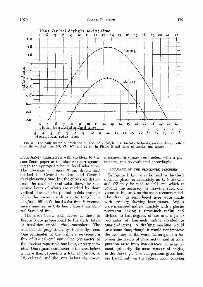
FIG. 3. The daily march of insolation outside the atmosphere at Lincoln, Nebraska, on two dates, plotted from the vertical lines Mj, a'k', b'P, and so on, in Figure 2 and times of sunrise and sunset.

immediately transferred with dividers to the coordinate paper at the abscissas corresponding to the appropriate hours, local solar time. The abscissas in Figure 3 are drawn and marked for Central standard and Central daylight-saving time, but the curves are drawn from the scale of local solar time, the successive hours of which are marked by short vertical lines at the plotted points through which the curves are drawn. At Lincoln, in longitude 96"43'W, local solar time is twenty- seven minutes, or 0.45 hour, later than Cen- tral Standard time.

The areas below such curves as those in Figure 3 are proportional to the daily totals of insolation outside the atmosphere. The constant of proportionality is readily seen. One centimeter of the ordinate represents a flux of 0.2 cal/cm2 min. One centimeter of the abscissa represents one hour, or sixty minutes. One square centimeter of the area below a curve then represents a total of 0.2(60), or 12, cal/cm2, and the area below the curve,

measured in square centimeters with a pla- nimeter, can be evaluated accordingly.

ACCURACY OF THE PROCEDURE DESCRIBED

In Figure 1, I o / p 2 may be read to the third decimal place, as accurately as I0 is known; and 02 may be read to 0.01 cm, which is beyond the accuracy of drawing such diagrams as Figure 2 on the scale recommended. The drawings reproduced here were made with ordinary drafting instruments. Angles were measured indiscriminately with a plastic protractor having a three-inch radius and divided to half-degrees of arc and a paper protractor of four-inch radius divided to quarter-degrees. A drafting machine would save some time, though it would not improve the accuracy of the work. Discrepancies between the results of construction and of computation arise from inaccuracies in measurement, primarily the measurement of angles, in the drawings. The comparisons given here are based only on the figures accompanying


this article, but they resemble the results of work with a few other drawings.

Computation of the hour angle of sunset, 0 0 , which with the opposite algebraic sign is the hour angle of sunrise, from

( 3 ) cos 0 0 = -tan 9 tan 6,

and its evaluation as time give for November 15 (Figure 2a) : sunrise, 0711, sunset, 1649; and for June 5 (Figure 2b): sunrise, 0434; sunset, 1926. In the former case the error is thus four minutes, in the latter three minutes of time, Both measurement and computation of h in Figure 2a give a value of 17'30'. In Figure 2b, measurement of h gives 48"10', computation 48"6', a difference too small to measure with the protractors used.

Planimetry of the area below the curves in Figure 3 made when these curves were drawn as fine pencil lines gave 384 cal/cm2 for No- vember 15 and 983 cal/cm2 for June 5. Com- putation of the daily total of radiation, Qb, from

(4) Q., = (144O/~) (1.952,'~') X ( w 0 sin 9 sin 6 + sin 00 cos 9 cos 6 ) ,

the integral of (1) over the daily cycle, in which T is the familiar ratio of the circum- ference of a circle to its diameter, 1440 is the number of minutes in twenty-four hours, and w0 is expressed in radians, gives 389 cal/cm2 for November 15 and 985 cal/cm2 for June 5. The errors are thus -1.3% and -0.2% respectively. They are acceptable for climatologic purposes.

GRAPHIC DERIVATION OF THE SUN'S AZIMUTH

The sun's azimuth at given times is fre- quently desired, as in connection with the exposure to the sun of walls that are not oriented with the cardinal directions. Dia- grams for finding it a t specific latitudes and on specific dates, which usually include the altitude as well, have been p ~ b l i s h e d . ~ Double interpolation for latitude and declination in these diagrams gives only very rough results. A graphic procedure analogous to that described for obtaining the sun's altitude is il-

4 A s in List, op. cit., footnote l, pp. 497-505, at intervals of five degrees of latitude and of declination.

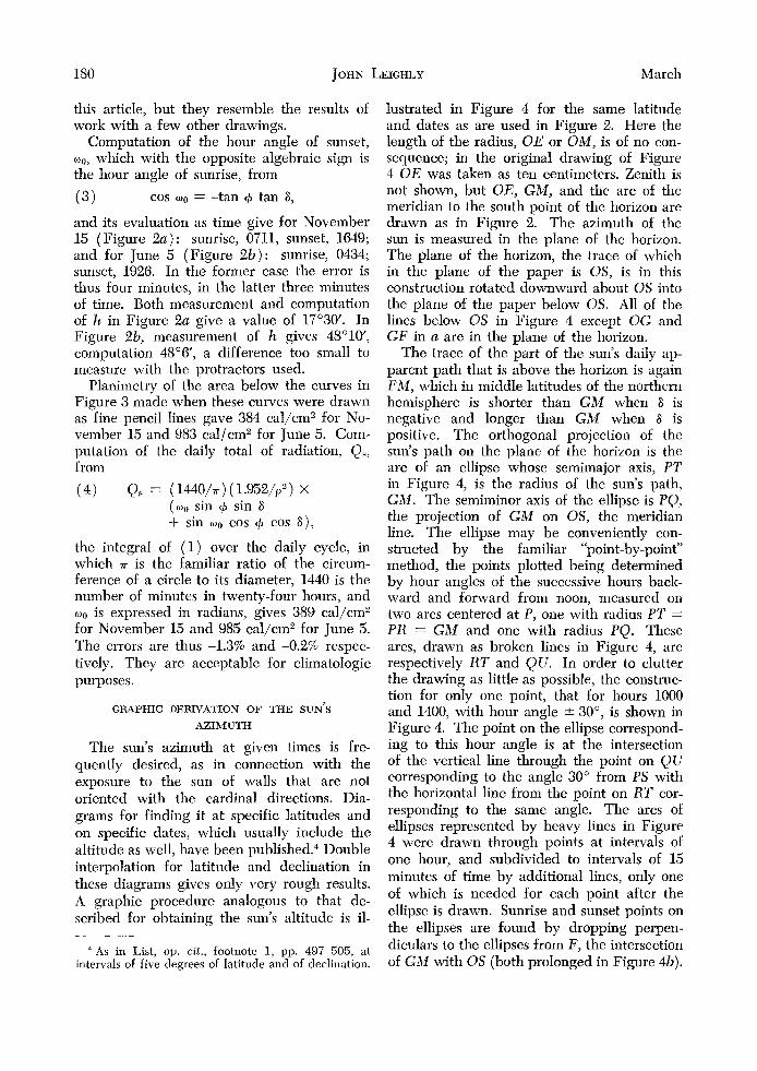
lustrated in Figure 4 for the same latitude and dates as are used in Figure 2. Here the length of the radius, OE or OM, is of no con- sequence; in the original drawing of Figure 4 OE was taken as ten centimeters. Zenith is not shown, but OE, GM, and the arc of the meridian to the south point of the horizon are drawn as in Figure 2. The azimuth of the sun is measured in the plane of the horizon. The plane of the horizon, the trace of which in the plane of the paper is OS, is in this construction rotated downward about 0s into the plane of the paper below 0s. All of the lines below 0 s in Figure 4 except OG and GF in a are in the plane of the horizon.

The trace of the part of the sun's daily apparent path that is above the horizon is again FLM, which in middle latitudes of the northern hemisphere is shorter than GM when 6 is negative and longer than GM when 6 is positive. The orthogonal projection of the sun's path on the plane of the horizon is the arc of an ellipse whose semimajor axis, PT in Figure 4, is the radius of the sun's path, GM. The semiminor axis of the ellipse is PQ, the projection of GM on OS, the meridian line. The ellipse may be conveniently constructed by the familiar "point-by-point" method, the points plotted being determined by hour angles of the successive hours back- ward and forward from noon, measured on two arcs centered at P, one with radius PT = PR = GM and one with radius PQ. These arcs, drawn as broken lines in Figure 4, are respectively RT and QV. In order to clutter the drawing as little as possible, the construction for only one point, that for hours 1 0 0 and 1400, with hour angle 2 30", is shown in Figure 4. The point on the ellipse corresponding to this hour angle is a t the intersection of the vertical line through the point on QU corresponding to the angle 30" from PS with the horizontal line from the point on RT corresponding to the same angle. The arcs of ellipses represented by heavy lines in Figure 4 were drawn through points at intervals of one hour, and subdivided to intervals of 15 minutes of time by additional lines, only one of which is needed for each point after the ellipse is drawn. Sunrise and sunset points on the ellipses are found by dropping perpendiculars to the ellipses from F , the intersection of GA4 with 0 s (both prolonged in Figure 4h).

1970 SOLAR CLIMATE

C

181

C .3

182 JOIIN LEICHLY March

19'70 SOLAR CLIMATE 183

Azimuths from the south point S are measured about 0 from 0s. These angles are indicated in Figure 4 for hours 9 and 15 by radii from 0 and arcs between 0s (prolonged) and these radii, drawn as broken lines. Azi- muths from north are obtained by adding 180" to these angles. Azimuths at sunrise and sunset are measured between 0 s (prolonged) and the radii from 0 to the sunrise-sunset points on the ellipses found by dropping perpendiculars from F. These radii and arcs are also drawn as broken lines in Figure 4. Azi- muths measured from OS, like hour angles, are positive in the afternoon and negative in the forenoon. Time may be safely interpolated in Figure 4 at least to intervals of five minutes.

The azimuths in Figure 4 are not quite so close to computed values as are altitudes in Figure 2. In a of the figure, measurement of the azimuth of the sun at 0900 and 1500 hours gives 45"10', computation 44'46', thus an error of +24'. In b, measurement gives 78"30', computation 78"5', error +2S. Azimuths of sunrise and sunset fare better, perhaps be- cause the construction required for finding them is simpler. In Figure 4a the measured value of azimuth from S of the sunrise-sunset point is 65"15', the computed value 65"28'; in 417 both measurement and computation give 120'20'.

Appendix: Mathematical Notes on the Constructions Described

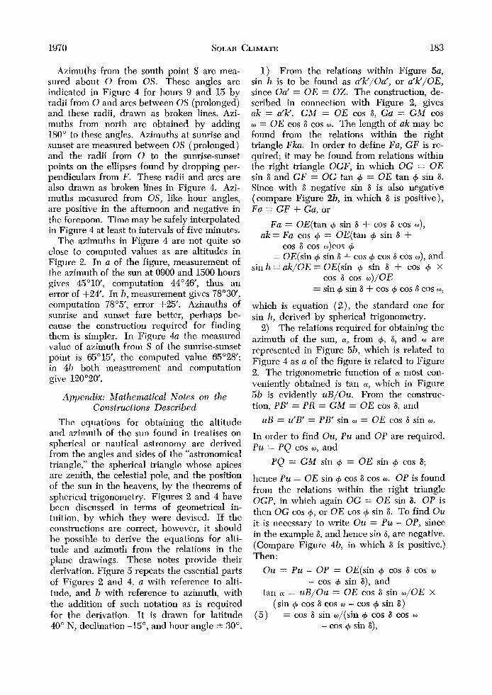
The equations for obtaining the altitude and azimuth of the sun found in treatises on spherical or nautical astronomy are derived from the angles and sides of the "astronomical triangle," the spherical triangle whose apices are zenith, the celestial pole, and the position of the sun in the heavens, by the theorems of spherical trigonometry. Figures 2 and 4 have been discussed in terms of geometrical in- tuition, by which they were devised. If the constructions are correct, however, it should be possible to derive the equations for altitude and azimuth from the relations in the plane drawings. These notes provide their derivation. Figure 5 repeats the essential parts of Figures 2 and 4, a with reference to altitude, and b with reference to azimuth, with the addition of such notation as is required for the derivation. It is drawn for latitude 40" N, declination -15", and hour angle f 30".

1) From the relations within Figure 5a, sin h is to be found as a'k'/Oa', or a'k'JOE, since Oa' = OE = 02. The construction, described in connection with Figure 2, gives ak = a'k'. GM = OE cos 6 , Ga = GM cos w = OE cos 6 cos W. The length of ak may be found from the relations within the right triangle Fka. In order to define Fa, GF is required; it may be found from relations within the right triangle OGF, in which OG = OE sin 6 and GF = OG tan b, = OE tan b, sin 6. Since with 6 negative sin 6 is also negative (compare Figure 2b, in which 6 is positive), Fa = GF + Gu, or

Fa = OE(tan b, sin 6 + cos 6 cos w), ak = Fa cos + = OE(tan b, sin 6 +

cos 6 cos 0)cos b, = OE(sin 9 sin 6 + cos + cos 6 cos w), and

sinh=akJOE= OE(sin b, sin 6 + cos b, x cos 6 cos w)/OE

= sin b, sin 6 + cos b, cos 6 cos W,

which is equation (2) , the standard one for sin h, derived by spherical trigonometry.

The relations required for obtaining the azimuth of the sun, a, from 4, 6 , and w are represented in Figure 5b, which is related to Figure 4 as a of the figure is related to Figure 2. The trigonometric function of a most conveniently obtained is tan a, which in Figure 5b is evidently u B / O u . From the construction, PB' = P R = GM = OE cos 6 , and

2)

uB = u'B' = PB' sin 0 = OE cos 6 sin u).

In order to find OIL, P u and O P are required. Pu = P Q cos W, and

P Q = GM sin b, = OE sin b, cos 6;

hence P u = OE sin 9 cos 6 cos W. O P is found from the relations within the right triangle OGP, in which again OG = OE sin 6. O P is then OG cos 4, or OE cos b, sin 6. To find Ou it is necessary to write Ou = P u - OP, since in the example 6, and hence sin 6 , are negative. (Compare Figure 4b, in which 6 is positive.) Then :

Ou = P u - O P = OE(sin b, cos 6 cos w - cos 4 sin S), and

tan N = u B / O u = OE cos 6 sin w/OE X

= cos 6 sin oJ(sin b, cos 6 cos w

- cos + sin 6 ) ,

(sin 9 cos 6 cos w - cos b, sin 6 ) ( 5 )


which is one equation from which ~r may be ~ b t a i n e d . ~

Figure 5 demonstrates a geometric relation that is not evident in Figures 2 and 4, but which makes it possible to construct both h and a in a single drawing. Ok in Figure 5a is equal to Ou in b of the same figure. Point k or u may be identified by imagining the position of the sun at any time projected horizon- tally onto the plane of the meridian and ver- tically onto the plane of the horizon, and lines then drawn to 0s perpendicular to 0s from

5Although I have not found ( 5 ) in a superficial examination of the literature, its reciprocal, as cot a, is given on p. 544 in E. Hammer, Lehr- und Hand- biich cler ebenen und sphicrischen Trigonowietrie (Stuttgart: J. B. Metzler, 1923), 5th edition. It may he readily obtained from equation ( 3 ) , p. lxviii, of R. S. Woodward, Smithsonian Geographical Tables, 3rd edition, 2nd reprint, Smithsonian Mi.vcellaneous Collections, 854 ( 1929 ), by a little algebraic manipu- lation.

the projected points in each of these planes. The perpendicular in the plane of the meridian intersects 0s in k, Figure 5a; the perpendicular in the plane of the horizon intersects 0s in u, Figure 5b. These points are identical; and the length of Ok or Ou is, by this reasoning, equal to OE cos h cos a. The line uB in Figure 5b is the continuation below 0s of ak in Figure 5u; the abscissas of points on the ellipses in Figure 4 corresponding to the respective hour angles may be obtained by dropping perpendiculars from points a, b, c, etc. on F M and continuing them downward below 0s. It is then necessary to draw only one additional line, such as B’B in Figure Sb, to locate each point, such as R, on QT. The result is, however, a confusing multiplicity of lines in the drawing unless the lines below 0s already used for finding h are erased before locating the points through which the ellipse is to be drawn.

Documents

GRAPHIC DERIVATION OF ELEMENTS OF THE SOLAR CLIMATE