Embed Size (px)
Citation preview

Grapher,·
User's Guide

GrapherTM Registration Information
Your Grapher product key is located in the email download instructions and in your account at MyAccount.GoldenSoftware.com.
Register your Grapher product key online at www.GoldenSoftware.com. This information will not be redistributed.
Registration entitles you to free technical support, download access in your account, and updates from Golden Software.
For future reference, write your product key on the line below.
_________________________________

GrapherTM User’s GuideThe Ultimate Technical Graphing Package
Golden Software, LLC809 14th Street, Golden, Colorado 80401-1866, U.S.A.
Phone: 303-279-1021 Fax: 303-279-0909www.GoldenSoftware.com

COPYRIGHT NOTICE
Copyright Golden Software, LLC 2018
The GrapherTM program is furnished under a license agreement. The Grapher software, user’s guide, and quick start guide may be used or copied only in accordance with the terms of the agreement. It is against the law to copy the software, user’s guide, or quick start guide on any medium except as specifically allowed in the license agreement. Contents are subject to change without notice.
Grapher is a registered trademark of Golden Software, LLC. All other trademarks are the property of their respective owners.
January 2018

Table of Contents
Chapter 1 - Introducing Grapher ................................................................................................ 1
System Requirements ............................................................................................................ 1
Installing Grapher ................................................................................................................. 2
Uninstalling Grapher .............................................................................................................. 2
Grapher Trial Functionality ..................................................................................................... 2
Scripter ................................................................................................................................ 3
New Features ....................................................................................................................... 3
Three-Minute Tour ................................................................................................................. 4
Grapher User Interface .......................................................................................................... 6
File Types ............................................................................................................................30
Plot Types ...........................................................................................................................32
Creating Graphs ...................................................................................................................35
Register Your Software .........................................................................................................37
Check for Update .................................................................................................................37
Technical Support ................................................................................................................38
Chapter 2 - Tutorial .................................................................................................................39
Tutorial Overview .................................................................................................................39
Advanced Tutorial Lessons ....................................................................................................39
A Note About the Documentation ...........................................................................................39
Starting Grapher ..................................................................................................................40
Lesson 1 - Viewing and Creating Data .....................................................................................40
Lesson 2 - Creating a Graph ..................................................................................................44
Lesson 3 - Modifying Plot Properties .......................................................................................45
Lesson 4 - Editing Axes .........................................................................................................48
Lesson 5 - Adding Additional Plots to the Graph .......................................................................54
Lesson 6 - Editing Graph Properties ........................................................................................56
Lesson 7 - Adding and Editing a Legend ..................................................................................58
Lesson 8 - Working with the Script Recorder ............................................................................61
Advanced Tutorial - Using the Magnifier ..................................................................................69
Advanced Tutorial - Using the Inset Zoom ...............................................................................73
Advanced Tutorial - Combining Plots from Different Graphs .......................................................76
Chapter 3 - Data Files and the Worksheet ..................................................................................79
Creating Data ......................................................................................................................79
Graphing and Viewing Data ...................................................................................................79
Data File Content .................................................................................................................79
Data File Formats .................................................................................................................79
Date/Time Formatting ...........................................................................................................80

Table of Contents
ii
Data in the Plot ....................................................................................................................86
List Worksheets ...................................................................................................................86
Display Worksheet................................................................................................................86
Auto Track Worksheets .........................................................................................................86
Reload Worksheets ...............................................................................................................87
Change Worksheets ..............................................................................................................87
Worksheet Window ...............................................................................................................88
Working with Worksheet Data ................................................................................................89
Paste Special .......................................................................................................................98
Import .............................................................................................................................. 100
Reload Data - Worksheet .................................................................................................... 101
Clear - Worksheet .............................................................................................................. 102
Insert - Worksheet ............................................................................................................. 102
Delete - Worksheet ............................................................................................................ 102
Find .................................................................................................................................. 103
Find Next .......................................................................................................................... 103
Replace ............................................................................................................................. 103
Find and Replace ................................................................................................................ 103
Format Cells ...................................................................................................................... 107
Column Width .................................................................................................................... 111
Row Height ........................................................................................................................ 113
Hiding Columns or Rows ..................................................................................................... 114
Sort - Worksheet ................................................................................................................ 115
Transform - Worksheet ....................................................................................................... 117
Mathematical Functions ....................................................................................................... 122
Statistics - Worksheet ......................................................................................................... 129
Transpose ......................................................................................................................... 142
Text To Number ................................................................................................................. 142
Number To Text ................................................................................................................. 143
Page Setup ........................................................................................................................ 144
Print ................................................................................................................................. 149
Chapter 4 - Creating Graphs ................................................................................................... 151
Creating Graphs in the Plot Window ...................................................................................... 151
Creating Graphs with the Graph Wizard ................................................................................ 151
Graph Wizard .................................................................................................................... 152
Creating Graphs from the Worksheet .................................................................................... 159
Creating Graphs Using Templates ......................................................................................... 160
Template Graphs ................................................................................................................ 160
Chapter 5 - Basic Type Plots ................................................................................................... 163
Line, Scatter, and Line/Scatter Plots ..................................................................................... 163

iii
Step Plots ......................................................................................................................... 167
Function Plots .................................................................................................................... 172
Bubble Plots ...................................................................................................................... 178
Class Scatter Plots .............................................................................................................. 184
3D Ribbon Plots and 3D Wall Plots ........................................................................................ 194
3D Step Plots ..................................................................................................................... 197
3D XYZ Plots ..................................................................................................................... 202
3D Function Plots ............................................................................................................... 206
XYZ Bubble Plots ................................................................................................................ 211
XYZ Class Scatter Plots ....................................................................................................... 217
Chapter 6 - Bar Type Plots ..................................................................................................... 223
Horizontal Bar Charts and Vertical Bar Charts ........................................................................ 223
Horizontal Category Bar Charts and Vertical Category Bar Charts ............................................. 224
3D Bar Charts .................................................................................................................... 225
XYZ Bar Charts .................................................................................................................. 226
Bar Chart Multiple Variable Data Files ................................................................................... 227
Plot Page - Bar Charts ......................................................................................................... 230
Bar Chart Groups ............................................................................................................... 238
Floating Bar Charts ............................................................................................................. 240
3D Floating Bar Charts ........................................................................................................ 241
XYZ Floating Bar Charts ...................................................................................................... 242
Plot Page - Floating Bar Charts............................................................................................. 243
Chapter 7 - Polar Type Plots ................................................................................................... 249
Polar Line Plot, Polar Scatter Plot, Polar Line/Scatter Plot ........................................................ 249
Polar Class Scatter Plot ....................................................................................................... 252
Polar Vector Plots ............................................................................................................... 262
Polar Function Plots ............................................................................................................ 265
Polar Bar Charts ................................................................................................................. 267
Bar Chart Groups ............................................................................................................... 271
Polar Rose Chart ................................................................................................................ 273
Polar Wind Charts .............................................................................................................. 279
Radar Charts ..................................................................................................................... 285
Chapter 8 - Ternary Plot Types ............................................................................................... 291
Ternary Line, Scatter, and Line/Scatter Plots ......................................................................... 291
Ternary Class Scatter Plots .................................................................................................. 295
Ternary Bubble Plots ........................................................................................................... 305
Piper Plot and Piper Class Scatter Plot ................................................................................... 312
Chapter 9 - Specialty Type Plots ............................................................................................. 317
High-Low-Close Plots .......................................................................................................... 317
Vector Plots ....................................................................................................................... 320

Table of Contents
iv
XYZ Vector Plots ................................................................................................................ 322
Plot Page - Vector Plots ....................................................................................................... 323
Stiff Plot ............................................................................................................................ 325
Chapter 10 - Statistical Type Plots .......................................................................................... 329
Histogram Plots.................................................................................................................. 329
3D Histogram Plots ............................................................................................................. 330
Plot Page - Histogram Plots ................................................................................................. 331
Box Plots ........................................................................................................................... 340
Pie Charts ......................................................................................................................... 350
3D Pie Charts .................................................................................................................... 351
Doughnut Plots .................................................................................................................. 352
3D Doughnut Plots ............................................................................................................. 353
Plot Page - Pie and Doughnut Charts .................................................................................... 354
Labels Page - Pie Charts and Doughnut Plots ......................................................................... 361
Q-Q Plots and Normal Q-Q Plots ........................................................................................... 363
Chapter 11 - Contour and Surface Type Plots ........................................................................... 367
Contour Data Map .............................................................................................................. 367
Contour Grid Map ............................................................................................................... 370
Contour Function Map ......................................................................................................... 374
Grid Properties - Contour Maps ............................................................................................ 377
Color Scale - Contour Maps ................................................................................................. 379
Levels - Contour Maps ........................................................................................................ 381
Surface Data Map ............................................................................................................... 384
Surface Grid Map ............................................................................................................... 388
Surface Function Map ......................................................................................................... 391
Grid Properties - Surface Maps ............................................................................................. 395
Color Scale - Surface Maps and Vector Plots .......................................................................... 397
Producing a Surface or Contour Map from a Regular Array of XYZ Data ..................................... 399
Inverse Distance to a Power ................................................................................................ 399
Chapter 12 - Fit Curves and Confidence Intervals ...................................................................... 401
Fit Plots ............................................................................................................................ 401
Available Fits ..................................................................................................................... 403
Orthogonal Polynomial Regression ........................................................................................ 406
Weighted Average Weights .................................................................................................. 410
Define Fit Equation ............................................................................................................. 411
Plot Page - Fit Plots ............................................................................................................ 413
Fit Statistics ...................................................................................................................... 418
Confidence Intervals ........................................................................................................... 422
Chapter 13 - Common Plot Properties ...................................................................................... 425
Error Bars ......................................................................................................................... 425

v
Data Limits Properties ......................................................................................................... 430
Labels Properties ................................................................................................................ 440
Label Format ..................................................................................................................... 452
Move Labels ...................................................................................................................... 455
Lighting Properties ............................................................................................................. 456
Symbol Properties .............................................................................................................. 458
Symbol Palette................................................................................................................... 464
Line Properties ................................................................................................................... 464
Line Palette ....................................................................................................................... 469
Line Styles ........................................................................................................................ 469
Fill Properties ..................................................................................................................... 474
Fill Palette ......................................................................................................................... 479
Fill Patterns ....................................................................................................................... 480
Color Gradient ................................................................................................................... 484
Color Table ........................................................................................................................ 490
Color Palette ...................................................................................................................... 492
Custom Colors ................................................................................................................... 493
Set Image Dialog ............................................................................................................... 496
Chapter 14 - Graph Properties ................................................................................................ 499
Title Properties .................................................................................................................. 499
3D Settings - Graph Objects ................................................................................................ 502
Graph Fill Properties ........................................................................................................... 503
Axis .................................................................................................................................. 506
Duplicate Axis .................................................................................................................... 506
Plot .................................................................................................................................. 507
Legend ............................................................................................................................. 509
Summation Plot ................................................................................................................. 521
Magnifier ........................................................................................................................... 524
Digitizing ........................................................................................................................... 526
Assign Coordinates ............................................................................................................. 528
Convert Graph or Plot ......................................................................................................... 529
Calculate Area ................................................................................................................... 530
Reset Rotation ................................................................................................................... 531
Chapter 15 - Axis Properties ................................................................................................... 533
Axis Limits ........................................................................................................................ 533
Types of Axes .................................................................................................................... 533
Standard Axes ................................................................................................................... 535
Angle Axes ........................................................................................................................ 537
Stiff Plot Axes .................................................................................................................... 541
Box Plot Axes .................................................................................................................... 541

Table of Contents
vi
Axis Properties ................................................................................................................... 542
Grid Lines .......................................................................................................................... 551
Tick Marks ......................................................................................................................... 553
Tick Labels ........................................................................................................................ 558
Select Date/Time ............................................................................................................... 571
Link Axis ........................................................................................................................... 572
Chapter 16 - Creating, Selecting, and Editing Objects ................................................................ 581
Text ................................................................................................................................. 581
Text Properties .................................................................................................................. 582
Polygon ............................................................................................................................. 603
Polyline ............................................................................................................................. 604
Symbol ............................................................................................................................. 605
Rectangle .......................................................................................................................... 606
Rounded Rectangle ............................................................................................................. 607
Ellipse ............................................................................................................................... 608
Spline Polyline ................................................................................................................... 608
Spline Polygon ................................................................................................................... 610
Reshape ............................................................................................................................ 611
Inset Zoom ....................................................................................................................... 613
Insert OLE Object ............................................................................................................... 615
Selecting Objects ............................................................................................................... 618
Metafile Properties .............................................................................................................. 621
Bitmap Properties ............................................................................................................... 622
Cut ................................................................................................................................... 623
Copy................................................................................................................................. 623
Paste ................................................................................................................................ 623
Paste Special ..................................................................................................................... 624
Copy Format ...................................................................................................................... 625
Paste Format ..................................................................................................................... 626
Undo ................................................................................................................................ 626
Redo................................................................................................................................. 626
Delete ............................................................................................................................... 626
Resize Objects ................................................................................................................... 627
Group ............................................................................................................................... 627
Layout Tab Commands ....................................................................................................... 630
View Tab Commands .......................................................................................................... 639
Chapter 17 - Importing, Exporting, and Printing Graphs and Graphics ......................................... 647
Open ................................................................................................................................ 647
Import .............................................................................................................................. 654
Save ................................................................................................................................. 657

vii
Save As ............................................................................................................................ 657
Save To Multi-Sheet Excel File ............................................................................................. 659
Export .............................................................................................................................. 662
Export Data ....................................................................................................................... 664
Export Data Points from the Plot .......................................................................................... 665
Page Setup ........................................................................................................................ 666
Print ................................................................................................................................. 667
Print Multiple ..................................................................................................................... 669
Chapter 18 - Options, Defaults, and Customizations .................................................................. 671
Options Dialog ................................................................................................................... 671
Defaults ............................................................................................................................ 688
Customizing Commands ...................................................................................................... 690
Chapter 19 - Automating Grapher ........................................................................................... 695
Script Recorder .................................................................................................................. 695
Scripter Windows ............................................................................................................... 696
Working with Scripts ........................................................................................................... 697
Writing Scripts ................................................................................................................... 698
Running Scripts.................................................................................................................. 699
Running Scripts from the Command Line ............................................................................... 699
Debugging Scripts .............................................................................................................. 700
Custom Script Buttons ........................................................................................................ 703
Object Browser .................................................................................................................. 704
Type Library References ...................................................................................................... 705
Scripter BASIC Language .................................................................................................... 705
Using Scripter Help ............................................................................................................. 721
Suggested Reading - Scripter .............................................................................................. 721
Grapher Object Model ......................................................................................................... 722
Appendix - File Formats ......................................................................................................... 745
File Format Chart ............................................................................................................... 745
Convert Older Grapher Files ................................................................................................. 752
Import File Types ............................................................................................................... 753
File Descriptions ................................................................................................................. 754
Import Options .................................................................................................................. 812
Import Automation Options ................................................................................................. 839
Export Options ................................................................................................................... 856
Export Automation Options .................................................................................................. 885
Index .................................................................................................................................. 907


1
Chapter 1 - Introducing Grapher
Welcome to GrapherTM, the easy-to-use 2D & 3D technical graphing package for scientists, engineers, business professionals, or anyone who needs to generate publication quality graphs quickly and easily. Grapher is an efficient and powerful graphing program for all of your most
complex graphing needs. Create exciting graphs and plots for presentations, papers, marketing, analysis, sales, and more. Capture the interest of your audience with 3D graphs.
With Grapher, creating a graph is as easy as choosing the graph type, selecting the data file, and clicking the Open button. Grapher automatically selects reasonable default settings for each new graph, though all of the graph settings can be modified. For example, you can change tick mark spacing, tick labels, axis labels, axis length, grid lines, line colors, symbol styles, and more. You can add legends, images, fit curves, and drawing objects to the graph. To apply the same custom settings to several graphs, you can create a Grapher template containing the preferred styles.
Automate data processing and graph creation using Golden Software's ScripterTM program or any
Active X automation program. Once the graph is complete, you can export it in a variety of formats for use in presentations and publications.
Grapher is extremely flexible. For example, you can combine multiple
plot types, display graph titles, customize axis settings, and more.
System Requirements The minimum system requirements for Grapher are:
Windows 7, 8 (excluding RT), 10 or higher
512MB RAM minimum for simple data sets, 1GB RAM recommended
At least 500MB free hard disk space
1024x768 or higher monitor resolution with a minimum of 16-bit color depth

Chapter 1 - Introducing Grapher
2
Installing Grapher Installing Grapher requires Administrator rights. Either an administrator account can be used to install Grapher, or the administrator's credentials can be entered before installation while logged in to a standard user account. If you wish to use a Grapher single-user license, the product key must be activated while logged in to the user account under which Grapher will be used. For this reason, we recommend logging into Windows under the account for the Grapher user, and entering the necessary administrator credentials when prompted.
Golden Software does not recommend installing Grapher 13 over any previous version of Grapher. Grapher 13 can coexist with older versions (e.g. Grapher 12) as long as they are
installed in different directories, which is the default.
To install Grapher from a download:
1. Log into Windows under the account for the individual who is licensed to use Surfer.
2. Download Grapher according to the emailed directions you received or from the My Products page of the Golden Software My Account portal.
3. Double-click on the downloaded file to begin the installation process.
4. Once the installation is complete, run Grapher.
5. License Grapher by activating a single-user license product key or connecting to a license server.
Uninstalling Grapher To uninstall Grapher, follow the directions below for your specific operating system. We
recommend deactivating your license prior to uninstalling Grapher if you are using a single-user license.
Windows 7
To uninstall Grapher, go to the Windows Control Panel and click the Uninstall a program link. Select Grapher 13 from the list of installed applications. Click the Uninstall button to uninstall Grapher 13.
Windows 8
From the Start screen, right-click the Grapher 13 tile and click the Uninstall button at the bottom of the screen. Alternatively, right-click anywhere on the Start screen and click All apps at the bottom of the screen. Right-click the Grapher 13 tile and click Uninstall at the bottom of the screen.
Windows 10
Select Settings in the Start menu. In Settings, select Apps | Apps & features. Select Grapher 13, and then click Unistall. To uninstall Grapher from the Windows Control Panel, click Programs
| Programs and Features. Next select Grapher 13 and click Uninstall.
Grapher Trial Functionality The Grapher trial is a fully functioning time-limited trial. This means that commands work exactly as the commands work in the full program for the duration of the trial. The trial has no further

3
restrictions on use. The trial can be installed on any computer that meets the system requirements. The trial can be licensed by activating a product key or connecting to a license server.
Scripter The Scripter program, included with Grapher, is useful in creating, editing, and running script files that automate Grapher procedures. By writing and running script files, simple mundane tasks or
complex system integration tasks can be performed precisely and repetitively without direct interaction. Grapher also supports ActiveX Automation using any compatible client, such as Visual BASIC. The automation capabilities allow Grapher to be used as a data visualization and map generation post-processor for any scientific modeling system.
The script recorder records commands in a script as you perform them in Grapher. Run the script, and Grapher repeats the steps. This is ideal for users that need to perform repetitive tasks but are unfamiliar with automation or for advanced users who do not want to manually enter all of the
syntax.
New Features This is an overview of some of Grapher 13's new features.
User Friendly
New and improved Graph Wizard makes creating graphs faster and easier for both new and
experienced users.
Redesigned ribbon makes commands much easier to find and use.
Redesigned the Property Manager to make finding properties easier and more intuitive.
Added a command and help topic search to the ribbon.
Plots are created with different colors when creating plots via the Graph Wizard, when
clicking Create in the New plot field of the Plot page, or when creating a multiple plots in one graph from the worksheet.
New default properties improve graph readability and appearance.
Improved the precision of page units.
Graph Features
Create Piper and Piper Class diagrams.
Angle ticks along grid lines to make reading Ternary and Piper diagrams easier.
Add a LOESS fit to scatter, line, and line/scatter plots.
Add a Reduced Major Axis fit to scatter, line, and line/scatter plots.
Calculate the standard error of the intercept and slope coefficients for linear, log, and exponential fit plots.
Calculate the correlation coefficient for fit plots.
Apply varying fill colors to all slices in a pie or doughnut plot with a colormap.
Multithreaded and optimized the gridding algorithm to display contour data maps and surface data maps faster.

Chapter 1 - Introducing Grapher
4
Drawing and Digitizing Features
Added over 150 complex line styles.
Automatically wrap words with the Text Editor.
Rotate images.
Import and Export Improvements
Import Vector PDF files
Import DGN Microstation Design v7 files
Import GeoJSON Data Interchange Format files
Import GML Geography Markup Language files
Import 000 IHO S-57 Electronic Navigation Chart files
Import RT* TIGER/Line files
Import TAB MapInfo Table vector files
Import VCT IDRISI Binary Vector files
Automation
Create piper and piper class diagrams.
Set the ternary axis tick mark direction.
Add a LOESS fit.
Add a Reduced Major Axis fit.
Three-Minute Tour We have included several sample files with Grapher so that you can quickly see some of
Grapher's capabilities. Only a few example files are discussed here, and these examples do not include all of Grapher’s many plot types and features. The Object Manager is a good source of information as to what is included in each file.
To view the sample files:
1. Open Grapher.
2. Select Sample Files in the Files list of the Welcome to Grapher dialog.
3. Select a sample file from the Sample Files list.
4. Click the Open button. The sample file is now displayed. Repeat as necessary to see the files of interest.
5. Click on various parts of the graph, axes, and plots in the Object Manager. View the object
properties in the Property Manager.

5
The piper class plot.grf sample file provides an example piper class plot with axis and graph titles, as well as a
class legend.
Using Grapher
Graphs can be created in several ways in Grapher. The Home | New Graph commands create a graph with a single plot, and then the Add to Graph commands can be used to add plots and features as desired. The Graph Wizard quickly creates a new graph with one or more plots from a
single data file. The Graph Wizard can also be used to add features to the graph, such as legends
and titles, as well as to apply a color palette to the plots in the graph.
To progress from a data file to a finished graph:
1. Create a data file. This file can be created in Grapher's worksheet window or outside of Grapher (using an ASCII text editor or Excel, for example).
2. Click the Home tab to select a graph type directly. For instance, click the Home | New Graph | Basic | Line Plot command.
3. In the Open Worksheet dialog, select the data file, and click Open. The graph is created from the selected data file, using default graph and plot properties.
4. Adjust the graph and plot properties using the Property Manager.
Using Scripter
Tasks can be automated in Grapher using Golden Software's Scripter program or any ActiveX Automation-compatible client, such as Visual BASIC. A script is a text file containing a series of instructions for execution when the script is run. Scripter can be used to perform almost any task in Grapher. You can do practically anything with a script that you can do manually with the mouse or your keyboard. Scripts are useful for automating repetitive tasks and consolidating a sequence of
steps. Scripter is installed in the same location as Grapher. Refer to the Grapher Automation help book for more information about Scripter. We have included several example scripts so that you can quickly see some of Scripter's capabilities.

Chapter 1 - Introducing Grapher
6
Example Script Files
A variety of script files are included with Grapher. You can run the script as is or you can customize the script.
To run a sample script in Grapher's Script Manager:
1. Open Grapher.
2. Check the View | Display | Script Manager command. A check mark will indicate the manager is displayed.
3. In the Script Manager, click the button.
4. In the Open dialog, select a sample .BAS file and click Open. The sample scripts folder is located at C:\Program Files\Golden Software\Grapher 13\Samples\Scripts by default. The script is displayed in the Script Manager.
5. Click the button to execute the script.
The axis properties.bas script edits all of the properties of an axis, including the tick marks,
grid lines, and breaking the axis.
To run a sample script in Scripter:
1. Open Scripter by navigating to the installation folder, C:\Program Files\Golden Software\Grapher 13. Double-click on the Scripter.exe application file.
2. Click the File | Open command and select a sample script .BAS file from the C:\Program
Files\Golden Software\Grapher 13\Samples\Scripts folder.
3. Click the Script | Run command to execute the script.
Grapher User Interface Grapher contains four document window types: the plot window, worksheet window, grid window, and Excel worksheet window. Graphs and maps are displayed and edited in the plot window. Tabular data files are displayed, edited, transformed, and saved in the worksheet window. A native
Excel workbook can be opened in the Excel window. Grid files can be viewed in the grid window. The Grapher user interface consists of the quick access toolbar, ribbon tabs and commands, tabbed documents, managers, and a status bar.

7
The Grapher user interface includes several managers and windows with a command ribbon at the
top.
The following table summarizes the function of each component of the Grapher layout.
Component Name
Component Function
Ribbon
The ribbon contains the tabs and commands used to run Grapher. Some
commands are unique to the plot document, worksheet document, and grid document.
Tabbed Windows
Multiple plot windows, worksheet windows, Excel worksheet windows and grid windows can be displayed as tabs. Click on a tab to display the window.
Plot Window The plot window contains the graphs and other graphics.
Worksheet Window
The worksheet window displays the contents of the plot data sources and data files.
Status Bar
The status bar shows information about the activity in Grapher. The status bar is divided into three sections that contain information about the selected command or object position, the cursor position, and the size of the selected object.

Chapter 1 - Introducing Grapher
8
Object Manager
The Object Manager contains a hierarchical list of objects in a Grapher plot window; these objects can be selected, arranged, and renamed in the Object Manager. The Object Manager is initially docked on the left side above the Property Manager.
Property Manager
The Property Manager lists the properties of a selected object. Multiple
objects can be edited at the same time by selecting all of the objects and changing the shared properties. The Property Manager is initially docked on the left side below the Object Manager.
Script Manager
The Script Manager controls scripts that are recorded and run within
Grapher. Right-click in the Script Manager to see relevant menu commands for opening, saving, and running scripts. The Script Manager is hidden by default.
Worksheet Manager
The Worksheet Manager contains a view of all data loaded into Grapher. Edits made in the Worksheet Manager are automatically reflected in the
graph. Right-click in the Worksheet Manager to save, edit, transform, sort, or obtain statistics on cells. When plots are first created or when they are opened from a GRF file, the data file contents is displayed in the Worksheet Manager. When a GPJ file is opened, the embedded data is displayed in the Worksheet Manager.
Opening Windows
Selecting the File | Open command opens any of the three window types, depending on the type of file selected. The File | Open Excel command opens an Excel file in a native Excel window inside Grapher, if possible. The File | New | Plot command creates a new plot window. The File | New | Plot from Template command opens a new plot window, based on an existing template file. The File
| New | Worksheet command creates a new worksheet window. The File | New | Template command creates a new plot window to use as a template file. The File | New | Excel Window opens a native Excel window inside Grapher, if possible.
Object Manager
When Grapher opens, the Object Manager is visible in the plot window by default. It contains a hierarchical list of the objects in the Grapher plot window. The Object Manager is initially docked at the left side of the window, giving the window a split appearance; however, it can be dragged and placed anywhere on the screen. The Object Manager can also be hidden as a tab, or displayed as a floating dialog.
Ribbon Tabs and Commands
All window types in Grapher include the ribbon that contains all Grapher commands. The ribbon is initially displayed in full size, but can be minimized by right-clicking on the ribbon and selecting
Minimize the Ribbon. The ribbon is then displayed in a method similar to menus in older versions of Grapher.
To customize the ribbon, right-click on the ribbon and select Customize the Ribbon. Select any command and click Add to add it to the selected ribbon tab on the left side of the dialog. Commands can only be edited in custom groups or on custom tabs.
Quick Access Toolbar
The Quick Access Toolbar is the toolbar at the top of the screen. This toolbar can be customized to include any commands. To customize the Quick Access Toolbar, right-click on the ribbon and select

9
Customize Quick Access Toolbar. Select any command and drag it to the desired place on the Quick Access Toolbar.
Tab View
The plot, worksheet, and grid windows are displayed as tabbed documents. When more than one window is open, tabs appear at the top of the document, allowing you to click on a tab to switch to a different window. The tabs may be dragged to reorder them. When a document contains unsaved
changes, an asterisk (*) appears next to its tabbed name. The asterisk is removed once the changes have been saved. Click the X on the tab to close that tab. If unsaved changes are in the document, a prompt to save the document appears.
Recent Documents
Use the numbers and file names listed on the right side of the File menu to open the most recently
used files. You can type a number that corresponds with the document or click on the document name to open it.
Click on any of the document names listed
in the Recent Documents list to open that file.

Chapter 1 - Introducing Grapher
10
To increase or decrease the number of files displayed in the list, change the number click on the File | Options command. On the General page, change the Recent files (restart required) option. The file list maximum is 16. The default is 10.
You can pin documents to the Recent Documents list. Pinned files will be moved to the top of the Recent Documents list and will not be removed as new files are added to the list.
To pin a file, click the gray pin to the right of the file name. The pin is displayed as , and the
file is pinned to the top of the Recent Documents list.
To unpin a file from the Recent Documents list, click the blue pin to the right of the file name.
The pin is displayed as , and the file is unpinned.
Plot Window
A plot window is the area used for creating and modifying graphs. When you first open Grapher, you can choose to start from an empty plot window. Multiple plot windows can be open at one time. Click the document tabs to easily move between multiple plot windows.
Plot Document Commands
File Opens, closes, saves, and prints files. Provides links to online references and email templates. Controls options and default settings. Provides access to licensing information and Grapher version number.
Home Contains the commands for creating graphs as well as some of the most commonly used commands.
Insert
Contains the commands for adding and editing drawn objects, OLE objects, images, and inset zoom objects.
Layout
Contains the commands for editing the page layout and printing options as well as the arrangement of the objects on the page.
View
Controls zoom, redraw, the window layout, and the display of managers,
status bar, tabbed documents, rulers, and drawing grid.
Automation Contains links to record or run a script and open the automation or BASIC language help files.
Graph Tools
Contains commands to modify and add items to graphs and plots.
The Application/Document Control menu commands control the size and position of the application
window or the document window.
Tab View
The plot, worksheet, and grid windows are displayed as tabbed documents. When more than one
window is open, tabs appear at the top of the document, allowing you to click on a tab to switch to a different window. The tabs may be dragged to reorder them. When a document contains unsaved changes, an asterisk (*) appears next to its tabbed name. The asterisk is removed once the changes have been saved.
11
Object Manager
The Object Manager contains a hierarchical list of the objects in a Grapher plot window. The
objects can be selected, arranged, and renamed in the Object Manager or with ribbon commands. Changes made in the Object Manager are reflected in the plot window, and vice versa.
Check the View | Display | Object Manager command to show or uncheck the command to hide the Object Manager. A check mark indicates the manager is visible. No check mark indicates the manager is hidden. You can also show or access the Object Manager by pressing ALT+F11.
The Object Manager contains a list of all objects in a plot window. The Object Manager can be used to
select objects, arrange objects, and control object visibility.
Object Visibility
Each item in the Object Manager list consists of an icon indicating the object type, a text label for the object, and a visibility check box. A check mark indicates that the object is visible. An empty
box indicates that the object is not visible. Click the check box to change the visibility of the item. Invisible objects do not appear in the plot window or on printed output.
Object Manager Tree
If an object contains sub-objects, a or displays to the left of the object name. Click the or
icon to expand or collapse the list. For example, a graph object contains a plot, e.g., line/scatter, plus at least two axes. To expand the tree, click on the icon, select the item and press the plus key (+) on the numeric keypad, or press the right arrow key on your keyboard. To collapse a branch of the tree, click on the icon, select the item and press the minus key (-) on the numeric
keypad, or press the left arrow key.
Selecting Objects
Click on the object name to select an object and display its properties in the Property Manager. The plot window updates to show the selected object with a selection bounding box and the status bar displays the name of the selected object. To select multiple objects, hold down the CTRL key and click on each object. To select multiple adjacent objects at the same level in the tree, click on the
first object's name, hold down the SHIFT key, and then click on the last object's name.

Chapter 1 - Introducing Grapher
12
Editing Object IDs
Select the object and then click again on the selected object (two slow clicks) to edit the object name. You must allow enough time between the two clicks so the action is not interpreted as a double-click. Enter the new name into the box. Alternatively, right-click on an object name and click Rename Object, select an object and click the Home | Selection | Rename command, or select an object and press F2. Enter a name in the Rename Object dialog and click OK to rename the object.
Arranging Objects
To change the display order of the objects with the mouse, select an object and drag it to a new position in the list above or below an object at the same level in the tree. The cursor changes to a black right arrow if the object can be moved to the cursor location or a red circle with a diagonal
line if the object cannot be moved to the indicated location. For example, a line/scatter plot can be moved anywhere within its graph object or into another graph object, but not into a group object.
Objects can also be arranged using the Layout | Move commands: To Front, To Back, Forward, and Backward.
The cursor changes to a black horizontal
arrow if an object can be moved to a new location in the Object Manager.
The cursor changes to a circle with a
diagonal line if an object cannot be moved to a new location in the Object Manager.

13
Deleting Objects
To delete an object, select the object and press the DELETE key. Some objects cannot be deleted. For example, you cannot delete an axis that is currently in use by a plot in a graph.
Keyboard Commands
Press ALT+F11 to access the Object Manager. Pressing ALT+F11 will also show the Object Manager if it is hidden or pinned.
Use the UP ARROW and DOWN ARROW keys to navigate between objects in the Object Manager. Hold CTRL to select multiple contiguous objects. Press LEFT ARROW or RIGHT ARROW to collapse or expand an item in the Object Manager such as a graph or group.
Press ALT+ENTER to access the Property Manager for the selected item. If the selected item cannot
be collapsed, such as a plot or axis, you can also press ENTER to access the object's properties. If the selected item can be collapsed, such as a group or graph, press ENTER to collapse or expand the item.
Property Manager
The Property Manager allows you to edit the properties of an object, such as a plot or axis. The
Property Manager contains a list of all properties for a selected object. The Property Manager can be left open so that the properties of selected objects are always visible.
When the Property Manager is hidden or closed, double-clicking on an object in the Object Manager, or pressing ALT+ENTER, opens the Property Manager with the properties for the selected object displayed. To turn on the Property Manager, check the View | Display | Property Manager command.
For information on a specific feature or property that is shown in the Property Manager, refer to the help page for that feature. For instance, if you are interested in determining how to set the Symbol column for a line/scatter plot or how to change the Foreground color for a bar chart, refer
to the specific pages for Symbol Properties or Fill Properties.
The Property Manager displays the properties
associated with the selected object.
Chapter 1 - Introducing Grapher
14
Expand and Collapse Features
Sections with multiple properties appear with a plus or minus to the left of the name. To expand a section, click on the button. To collapse a section, click on the icon. For example, the expanded End Styles section contains three properties: Start, End, and Scale.
Changing Properties
The Property Manager displays the properties for selected objects. To change a property, click on
the property's value and type a new value, scroll to a new number using the buttons, select a
new value using the slider, or select a new value from the list or palette. For example, a polyline has Style, Color, Opacity, and Width properties and an End Styles sub-section with Start,
End, and Scale properties. Changing the Color requires clicking on the current color and selecting a new color from the color palette. Changing the Opacity requires typing a new value or clicking on the slider bar and dragging it left or right to a new value. Changing the Width requires typing a new number or scrolling to a new number. Changing the End requires clicking on the existing style and
clicking on a new style in the list.
The selections in the Property Manager control which properties are displayed. Properties are hidden when they do not have an effect on the object. For example when the Gradient is set to None on the Fill page, the Colormap and Fill orientation properties are hidden. When the Gradient is
changed to Linear, the Colormap and Fill orientation properties are displayed, while the Pattern, Foreground color, and Foreground opacity properties are hidden.
You can modify more than one object at a time. For example, click on X Axis 1 in the Object Manager, and then hold the CTRL key and click Y Axis 1. You can change the properties of each axis simultaneously in the Property Manager. Only shared properties may be edited when multiple objects are selected. For example, only the line properties are displayed when both a polyline and polygon are selected. You can edit multiple plots of the same type at one time. However, no properties are displayed when the selected plots are different plot types.
Applying Property Manager Changes
Object properties automatically update after you select an item from a palette, press ENTER, or
click outside the property field. When using the buttons or slider, changes are displayed on the
graph immediately.
Keyboard Commands
Press ALT+ENTER to access the Property Manager. Pressing ALT+ENTER will also show the Property Manager if it is hidden or pinned. When working with the Property Manager, the up
and down arrow keys move up and down in the Property Manager list. The TAB key activates the highlighted property. The right arrow key expands collapsed sections, e.g., Plot Properties, and the left arrow collapses the section.
CTRL+A can be used to select all of the contents of a highlighted option, such as the function plot's Y = F(X) = equation. CTRL+C can be used to copy the selected option text. CTRL+V can be used to paste the clipboard contents into the active option.
Property Defaults
Use the File | Options command to change the default rulers and grid settings, digitize format, line, fill, symbol, and font properties. Use the File | Defaults command to set the default values for base

15
objects, graphs, line type plots, bar type plots, 3D XYY plots, 3D XYZ plots, maps, other plots, axes, legend, wind chart legends, and class plot legends.
Property Manager Information Area
If the Display Property Manager info area is checked on the File | Options | Display page, a short help statement for each selected command in the Property Manager.
Worksheet Manager
The Worksheet Manager contains a view of all data loaded into Grapher. Multiple data files are displayed in a tabbed format. By default, the Worksheet Manager appears at the right of the Grapher window.
Right-click inside the Worksheet Manager to open the worksheet menu commands. These
commands are named similarly to the commands on the ribbon. Use the Home | New Graph commands to create a graph in the current plot window. Use the Data Tools menu commands to transform, sort, or generate statistics for the worksheet data.
Right-click in the Worksheet Manager to access all
worksheet menu commands.
Check the View | Display | Worksheet Manager command to show or clear the box to hide the Worksheet Manager. A check mark indicates the manager is visible. No check mark indicates the manager is hidden.

Chapter 1 - Introducing Grapher
16
You can see all data used in all open plot windows in
the Worksheet Manager.
Script Manager
The Script Manager allows you to work with automation within Grapher rather than opening Golden Software's automation program, Scripter, separately. All of Scripter's functionality is available within the Script Manager. Right-click in the Script Manager to access Scripter's menu commands.
By default, the Script Manager is not displayed. Click the View | Display | Script Manager command to show or hide the Script Manager. A check mark indicates the manager is visible. No check mark indicates the manager is hidden. When the Script Manager is displayed, the default
location is tabbed with the Worksheet Manager.
The Script Manager is used to view, record, edit, and run scripts.
Script Manager Menu Commands
Right-click in the Script Manager window to access the following menu commands.
File Create, open, close, save, and print scripts
Edit
Undo and redo changes; copy and paste changes; change formatting;
find and replace specific text; call out various script commands; edit a UserDialog; and edit script references

17
View View or hide macros, windows, toolbar, status bar, and edit buttons; view and change font and tab spacing; view or hide object and proc lists
Macro Run, pause, or end a macro
Debug Navigate statements; toggle and clear break points; watch and add expressions; view the selected objects methods and properties
Sheet Open Uses statements, close statements
Help Display help for WinWrap Basic, Basic language, and the selected word; display information about WinWrap Basic
The Application/Document Control menu commands control the size and position of the application window or the document window.
Changing the Window Layout
The managers display in a docked view by default. However, they can also be displayed as floating windows. The visibility, size, and position of each manager may also be changed.
Manager Visibility
Use the View | Display commands to show or hide the Object Manager, Property Manager, Script Manager, Worksheet Manager, and Status Bar. A check mark indicates the manager is displayed.
An empty check box indicates the manager is closed. Alternatively, you can click the button in the title bar of the manager to close the manager window.
Auto-Hiding Managers
Click the button to auto-hide a docked manager. The manager slides to the side or bottom of the
Grapher main window and a tab appears with the window name. You can increase the plot document space by minimizing the managers with the Auto Hide feature. To hide the manager, click
the button in the upper right corner of the manager. When the manager is hidden, place the
cursor directly over the tab to display the manager again. Click the button to return the manager to its docked position.
The Object Manager appears as a
tab on the side of the window.
Size
Drag the sides of a floating plot window, worksheet window, manager, toolbar, or menu bar to change its size. If a window or manager is docked, its upper and lower bounds are indicated by a
or cursor. Move the cursor to change the size.

Chapter 1 - Introducing Grapher
18
Position
To change the position of a docked manager, click the title bar and drag it to a new location. A thick light gray rectangle indicates that the manager is floating.
Docking Managers
Grapher has a docking mechanism feature that allows for easy docking of managers. Left-click the title bar of a manager and drag it to a new location while holding down the left mouse button. The docking mechanism displays arrow indicators as you move the manager around the screen. When the cursor touches one of the docking indicators in the docking mechanism, a blue rectangle shows the window docking position. Release the left mouse button to allow the manager to be docked in the specified location. Double-click the title bar of a manager to switch between the docked and floating positions.
The docking mechanism makes it easy to position managers.
Tabbed Managers
To create tabbed managers:
1. Left-click the title bar of the manager and drag over the other manager. A docking mechanism will be displayed.
2. Hover the cursor over the center of the docking mechanism. The blue rectangle shows where the tabbed manager will display.
3. Release the mouse button.
To return to individual managers from the tabbed view:
1. Click on the manager's name on the tab.
2. Drag the tab to a new position.
Click on the manager's tab and drag the cursor
to a new position to separate the managers.
Restoring the Managers to Their Default Locations
If the managers have moved or become invisible, or if they are in undesired locations, you can use the View | Display | Reset Windows command to move them back to their original locations. You must restart Grapher for the changes to take effect.

19
Status Bar
The status bar is located at the bottom of the window. Check or clear the View | Display | Status Bar command to show or hide the status bar. The status bar displays information about the current command or selected object in Grapher. The status bar is divided into three sections. The left section shows the selected object name. If a menu command is selected, a brief description of the
command appears in the left section. The middle section shows the cursor coordinates in page units. The middle section also displays the graph's X and Y coordinates when using the Graph Tools | Digitize commands or when the Display value on click option is selected in the Options dialog. The right section displays the dimensions of the selected object.
In the Script Manager, the status bar contains current command progress on the left and the script line number on the right.
Worksheet Window
The worksheet window contains commands to display, edit, enter, and save data. The worksheet window has several useful and powerful editing, transformation, and statistical operations available. Several import and export options are available for opening data files from other spreadsheet programs. The Data Tools tab is automatically selected when you open or switch to a worksheet document.
Worksheet Commands
Some commands are not available when viewing a worksheet. For example, none of the Insert and Layout commands are available and only a few of the Home and View commands are available.
File Opens, closes, saves, imports, exports, and prints files. Provides links to online references and email templates. Provides access to licensing information and Grapher version number.
Home Contains clipboard, undo, and graph creation commands.
View
Controls the display of toolbars, managers, status bar, tabbed documents, and the window layout.
Automation Contains links to record or run a script and open the automation or BASIC language help files.
Data Tools Contains commands for modifying the worksheet appearance, editing the data file, and analyzing the data.
The Application/Document Control menu commands control the size and position of the application window or the document window.

Chapter 1 - Introducing Grapher
20
Worksheet Window
To enter data in a worksheet, use the File | Open command to open an existing data file or click the File | New | Worksheet command to create a blank worksheet. Data already used to create plots can be opened in the worksheet window with the Graph Tools | Worksheet | Display command.
The components of the worksheet window are discussed below.
The components of a worksheet window shown above are described in the following table.
Column Letters The column letters identify a column in the worksheet.
Row Numbers The row numbers identify a row in the worksheet.
Active Cell
The active cell is highlighted with a bold outline. The active cell receives
data input (numeric values or text strings) from the keyboard. Only one cell is active at a time.
Active Cell Location
The active cell location is specified by column letter and row number.
Active Cell Edit Box
The active cell edit box displays the contents of the active cell. Data
typed into an empty cell appears in both the edit box and the active cell.
Worksheet Name The worksheet name displays the data file name or the worksheet number if the data file has not been saved.
Select Entire Worksheet Button
The select entire worksheet button is used to select all cells in the worksheet.
Grid Document
The grid window contains the commands for viewing the XYZ value of grid nodes and displaying contour lines. Each grid node is indicated with a "+" in the grid window by default. The active node is highlighted with a red diamond. To move between grid nodes, press the arrow keys, or left-click
a node to make it the active node. The Grid tab is automatically selected when you open or switch to a grid document.
Some commands are not available when viewing a grid file. For example, none of the Insert and Layout commands are available and only a few of the Home and View commands are available.
Grid Document Commands
21
File Opens, closes, saves, imports, exports, and prints files. Provides links to online references and email templates. Provides access to licensing information and Grapher version number.
Home Contains commands for creating graphs and links to the tutorial and help file.
View
Controls the display of toolbars, managers, status bar, tabbed documents; and the resetting of the window layout.
Automation Contains links to record or run a script and open the automation or BASIC
language help files.
Grid Tools Controls the display of the grid window and contour levels and displays grid information
The Application/Document Control menu commands control the size and position of the application window or the document window.
Show Contours
Check the Grid | Display | Contours command in the Grid Document to turn on the display of contour lines on the map. When the command is checked, the contours are displayed on the map. When the command is not checked, the contours are not displayed on the map. Click on the command to toggle between showing and hiding contours.
Show Nodes
Check the Grid Tools | Display | Nodes command in the Grid Document to turn on the display of
grid node markers on the map. When the command is checked, a "+" appears at the location of each grid node. When the command is not checked, the "+" signs are not shown. Some node markers are not displayed if the zoom or density is such that they are too close. Although not all of
the markers are shown, the active node indicator still "snaps" to each grid node as the arrow keys and mouse are used.
Grid Information
In the grid document, use the Grid Tools | Options | Grid Info command to open a dialog with Grid Information. The Grid Information can also be accessed in the plot window by selecting the grid based map and clicking on the words <Click here to display grid information> in the
Property Manager.
The Grid Information displays the following information
Date the grid information was created
Grid file name
Total Nodes
Filled Nodes
Blanked Nodes
Grid Geometry
X Maximum
X Spacing
Y Minimum
Y Maximum

Chapter 1 - Introducing Grapher
22
Y Spacing
Grid Statistics
Z Minimum
Z 25%-tile
Z Median
Z 75%-tile
Z Maximum
Z Midrange
Z Range
Z Interquartile Range
Z Median Abs. Deviation
Z Mean
Z Trim Mean (10%)
Z Standard Deviation
Z Variance
Z Coef. of Variation
Z Coef. of Skewness
Z Root Mean Square
Z Mean Square
Large Grid Files
If the grid file is large, a message box appears. Click the OK button to create a detailed report, or click the Cancel button to create a shorter, less detailed report.
Save and Print
Use the File | Save command to save the grid information as a [.RTF] or [.TXT] file or use the File | Print command to print the grid information for reference.
Tabbed Documents
In a plot window, click the File | Options command. In the Options dialog, on the left side, click on Display. On the right side, check the Tabbed documents command to display plot, worksheet, and grid windows as tabbed documents rather than the traditional multiple document interface.
When viewing in tabbed document mode, the tabs may be dragged to reorder them. The left/right
arrow buttons at the right of the tabs are used to scroll the tabs should there be more tabs than
can fit along the top of the window.
Plot 1, Worksheet1, Plot2, and Worksheet2 are tabbed.
The left and right arrows are used to scroll.

23
When a document contains unsaved changes, an asterisk appears next to its tabbed name. The asterisk (*) disappears once the unsaved changes have been saved.
Ribbon
The Ribbon is the strip of buttons and icons located above the plot, worksheet, and grid windows. The Ribbon replaces the menus and toolbars found in earlier versions of Grapher. The ribbon is designed to help you quickly find the commands that you need to complete a task.
Above the Ribbon are a number of tabs, such as Home, Automation, and Graph Tools. Clicking
or scrolling to a tab displays the options located in this section of the ribbon. The tabs have commands that are organized into a group. For instance, all the script related commands are on the Automation tab.
The Ribbon is displayed with the Home tab selected.
Minimizing the Ribbon
The ribbon can be minimized to take up less space on the screen. To minimize the ribbon, right-click on the ribbon and select Minimize the Ribbon or click the button in the top right portion of the Grapher window. When displayed in a minimized mode, only the tabs at the top of the screen
are visible. To see the commands on each tab, click the tab name. After selecting a command, the
ribbon automatically minimizes again.
The Ribbon displayed with the Minimize the Ribbon option selected. Clicking any tab name displays
the ribbon.
Command and Help Search
The ribbon also includes a command search to the right of the last tab (Automation, Graph Tools, Data Tools, or Grid Tools depending on document type). Begin typing a command name to search for commands. Click on a command in the search results to use the command. Press ENTER to quickly use the top search result command. For example type "add" into the command search
bar and the Add Plot, Add Axis, and Add Legend commands are displayed in the search results. You
can also click Search help file at the bottom of the results list to search the help file for the search term.
The command search will return commands from all ribbon tabs. No more than five commands are displayed in the results list. A command may be disabled in the results list if the command is not applicable to the current document or selection.

Chapter 1 - Introducing Grapher
24
Reset the Ribbon
To reset all customizations on the ribbon, click the Reset button at the bottom of the Customize Ribbon dialog.
Quick Access Toolbar Commands
The Quick Access Toolbar is at the top of the Grapher window. This toolbar has frequently used commands and can be customized by the user. The commands in the Quick Access Toolbar are the same regardless of the type of window displayed in Grapher.
The Quick Access Toolbar is displayed
at the top of the Grapher window.
Displaying the Quick Access Toolbar Below the Ribbon
To display the Quick Access Toolbar below the ribbon, right-click on the ribbon and select Show Quick Access Toolbar Below the Ribbon. This setting is useful if you have added many commands to the Quick Access Toolbar. More commands display, by default, when the Quick Access
Toolbar is below the ribbon. When combined with the minimized ribbon appearance, this can give single click access to all your most used commands and maximize the viewing area for the plot.
Customize the Quick Access Toolbar to display all the commands you frequently use. Then, display the Quick Access Toolbar below the ribbon bar. When the ribbon bar is minimized, it appears that all of your commands are in a single toolbar, ready to create what you want with a single click.
Keyboard Commands
Keyboard commands can be used to increase efficiency and precision in the Grapher environment.
Plot Window
You can use the keyboard to move the pointer within the plot window, to select and move objects, and perform commands.
The ARROW keys move the pointer within the plot window when no object is selected.
The ARROW keys move selected objects.
Press CTRL+TAB to change switch between document windows.
Pressing the SPACEBAR is equivalent to clicking the left mouse button.
"Double-clicking" the SPACEBAR by pressing the spacebar twice is the same as double-
clicking the mouse.
Press SHIFT+SPACEBAR to deselect all objects.

25
Manager Access
Press ALT+ENTER to activate the Property Manager
The ARROW keys move between properties in the Property Manager.
Press ALT+F11 to activate the Object Manager
The ARROW keys move the selection in the Object Manager.
Tab Commands Access
The keyboard can be used to access the menu commands.
Press the ALT key and press any letter or number that appears in a box to indicate the
desired ribbon tab.
When the appropriate tab is displayed, you can access a command by pressing the letter or
number that appears in a box to indicate the desired command.
Press ALT and the ARROW keys on the keyboard to switch between ribbon tabs.
Dialog Access
You can also use the keyboard to move around in a dialog.
The TAB key moves between the options in the dialog. As you use the TAB key to move through the dialog, the options are highlighted as they become active.
The SPACEBAR is used to simulate mouse clicks, allowing you to toggle check boxes or press
buttons that provide you with access to other dialogs or close the current dialog.
You can also use the underlined hotkeys by holding down the ALT key and typing the letter.
This moves you immediately to the desired option. Note that not all of the dialogs have ALT key access.
General Commands
These keyboard commands are used in the plot or worksheet windows.
File
CTRL+N Open a new plot window
CTRL+W Open a new worksheet window
CTRL+O Open a file
CTRL+S Save a Grapher .GRF file
CTRL+I Import a file into the plot window
CTRL+E Export the plot window to a file
CTRL+P Print the drawing in the current plot window or print the worksheet contents
ALT+F4 Close Grapher
Home
CTRL+V Paste the clipboard contents into the plot window or worksheet
CTRL+X Cut the selected objects to the clipboard
CTRL+C Copy the selected objects to the clipboard

Chapter 1 - Introducing Grapher
26
CTRL+SHIFT+C Copy the format of the selected object
CTRL+SHIFT+V Paste the format of the object to the newly selected objects
CTRL+Z Undo the last command
CTRL+Y Redo the previous undo command
F1 Open help
View
CTRL+D Zoom so all objects fill the plot window
CTRL+L Zoom in on selected objects so they fill the view
CTRL+G Zoom to the extents of the page
F11 Zoom to the full screen
CTRL++ Zoom in twice the scale at the center of the screen
CTRL+- Zoom out twice the scale from the center of the screen
CTRL+R Zoom on a selected rectangle
F5 Redraw the screen
Arrange
CTRL+A Select all the objects in the plot window
CTRL+SHIFT+A Deselect all the objects in the plot window
F2 Rename the selected object
DELETE Delete the selected objects in the plot window, clear cells in the worksheet
CTRL+PAGE DOWN Move selected object backward
SHIFT+PAGE DOWN Move selected object to back
CTRL+PAGE UP Move selected object forward
SHIFT+PAGE UP Move selected object to front
Application Control Window
CTRL+F4 Close the plot or worksheet window
ALT+F4 Close Grapher
ALT+SPACE Display the application control menu
ALT+HYPHEN Display the document window control menu
CTRL+F6 Next document window
CTRL+SHIFT+F6 Previous document window
CTRL+TAB Switch between Grapher windows
ALT or F10 Activate the tabs in the ribbon
CTRL+ESC Display the Windows start menu
ALT+TAB Switch to the last active application

27
Worksheet Commands
These keyboard commands are specific to the worksheet.
F2 Edit active cell
ARROW KEYS Move to adjacent cell
ENTER Preserve the typed contents in the cell
HOME Go to the first row containing data in the selected column
END Go to the last row containing data in the selected column
PAGE UP Scroll the table up by the number of visible rows
PAGE DOWN Scroll the table down by the number of visible rows
TAB Move the active cell right one column
CTRL+HOME Move the active cell to the top cell of the left most column
CTRL+END Move the active cell to the bottom occupied row and right most column
Maximize the Plot Window Display Space
Several options exist to maximize the plot window display space. See some common options below.
One of the easiest ways of maximizing the plot window display space is to turn on only the managers that you use. To turn off other managers, click the View tab in the ribbon. In the Display section, uncheck the boxes for the managers that you do not regularly use. For instance, if you do not use the Script Manager or Worksheet Manager, unchecking these options will
provide much additional space.
To temporarily turn the display of all of the managers off, click the View | Display | Hide All command. To turn the display of all of the managers back on, click the View | Display | Show All command. Alternatively, check only those managers that you want to see.
The ribbon can be minimized so that the tab names appear more like menus instead of tabs. To minimize the ribbon, right-click on the ribbon and select Minimize the Ribbon. When displayed in a minimized mode, only the tabs at the top of the screen are visible. To see the commands on each tab, click the tab name. After selecting a command, the ribbon automatically minimizes again.
Welcome to Grapher Dialog
When Grapher is first opened, the Welcome to Grapher dialog appears. The Welcome to Grapher dialog provides a way to start Grapher in your desired method. Whatever option is
selected becomes the default for all future Grapher sessions. The dialog reappears every time Grapher opens.

Chapter 1 - Introducing Grapher
28
The Welcome to Grapher dialog appears when you open Grapher.
New Options
The New list, on the left side of the dialog, controls the default setting and the method that this instance of Grapher will begin with.
Click any of the buttons to open Grapher using the method described. For instance, click the Plot + Worksheet option to open Grapher with a new empty plot window and new empty worksheet window. Available options are Plot + Worksheet, Plot, Template, Worksheet, Plot from Template, and Plot from Wizard.
Plot + Worksheet opens a new empty plot window and new empty worksheet window. This is how older versions of Grapher always opened. This is similar to using the File | New | Plot
command and the File | New | Worksheet command or clicking the and buttons.
Plot opens a new empty plot window. This is similar to using the File | New | Plot command
or clicking the button.
Template opens a new empty template window. A template can be saved and used later to
create graphs with the same basic settings. This is similar to using the File | New | Template command.
Worksheet opens a new empty worksheet window. This is similar to using the File | New |
Worksheet command or clicking the button.
Plot from Template creates a new empty plot window from an existing template. This is similar to using the File | New | Plot from Template command. After clicking the Plot from
Template button, the Open dialog appears. Select the Grapher template GRT file and click
Open. Select each data file required to open the template and click Open. The template appears with the desired data.
Plot from Wizard opens a new empty plot window with the graph wizard dialog open. This is
similar to using the Graphs | Create | Graph Wizard command. This allows an easy method to create a default graph. The wizard has settings to create every plot type.

29
Default Method
After clicking any of the buttons in the New list, the selected button is written to the Grapher program as an option. Every time the program is opened, this default option will be used if you click the Close button or the X button in the top right. In addition, this default method is used if the Welcome to Grapher dialog is not displayed.
To change the default method, open any plot window. Click the File | Options command. On the left side of the dialog, click General. On the right side of the dialog, change the Start up action. Available options match the options included as buttons in the Welcome to Grapher dialog. In addition, the option Do nothing exists from the Options dialog.
Files List and Preview
The Files list, in the middle of the dialog, contains options to open specific files. Click the current file type selection and select the desired file type from the list. Available options are Recent Files,
Sample Files, Project Files, Script Files, and Browse. Select the desired option and the list updates
to show all files in the selected type. Data files are not listed in this section. To open a data file, select Browse in the file type list.
Recent Files lists the most recent 10 files that have been opened in Grapher. This is similar
to the file list under the File menu. Click on any file in the list and click the Open button to close the Welcome dialog and open the selected file. The number of recent files displayed in the list can be changed in the File | Options dialog. Files that are pinned to the Recent Documents list will be displayed at the top of the Recent Files list, including pinned data files.
Sample Files lists all of the GRF and GPJ files in the Grapher Samples directory. This is C:\Program Files\Golden Software\Grapher 13\Samples, by default. Click on any file in the list and click the Open button to close the Welcome to Grapher dialog and open the
selected file.
Project Files lists all of the GRF, GPJ, and GRT files in the selected directory. After clicking
Project Files the first time, a Select Folder dialog appears. Select the directory on the
computer that should be used as the Project Files directory and click Select Folder. All of the GRF, GPJ, and GRT files from the selected directory are listed. Click on any file in the list and click the Open button to close the Welcome to Grapher dialog and open the selected file. Click the Set Project Folder button to change the directory, or change the project folder directory in the File | Options dialog.
Script Files lists all of the BAS files in the project folder. After clicking Script Files the first time, a Select Folder dialog appears. Select the directory on the computer that should be used as the Project Files directory and click Select Folder. All of the BAS files from the
selected directory are listed. Click on any file in the list and click the Open button to close the Welcome dialog. The script is displayed in the Script Manager and run. Any plots or worksheets that are opened or created from the plot are created. Click the Set Project Folder button to change the directory, or change the project folder directory in the File | Options dialog.
Browse opens the Open dialog, where you can select the file to open to start this instance of Grapher. To start Grapher with a file that is not in the Recent Files list, Sample Files list, or
Project Folder, or to open a data file, select Browse.
Click a file name to select to file. A preview of the selected file is displayed, and the selected file can
be opened by clicking the Open button. Click on another file or press the UP ARROW or DOWN ARROW keys to change the file selection.
Project Folder
Clicking the Set Project Folder button opens the Select Folder dialog. The Browse for Folder dialog will open for Windows XP users. The selected directory is used for the Project Files and Script

Chapter 1 - Introducing Grapher
30
Files file lists. The Project Folder can also be changed in the File | Options dialog. If the Project Folder specification is removed in the Options dialog, the Windows default (C:\Users\<username>\Documents) folder is used until a new project folder is selected.
Open
After clicking on a file in the file type list, click the Open button to open the selected file. The Welcome to Grapher dialog closes and the action is performed. The Open button is disabled until a file is selected in the Files list. To open a file that is not located in any of the lists, or to open a data file, select Browse in the file type list.
Tips
The Welcome dialog displays a useful tip on the right side of the dialog.
Start with the Tutorial
Click the Tutorials button to start Grapher with a new plot and worksheet and the help open to the Tutorial Introduction topic.
Turn Welcome Dialog Off
The Show this dialog at start up check box is checked by default. Click the Show this dialog at startup to remove the check and open Grapher without the Welcome to Grapher dialog in all future instances. After closing Grapher and reopening, the Welcome to Grapher dialog will not be displayed.
This option can be changed by clicking the File | Options command. In the Options dialog, click on Dialog Messages on the left side. On the right side, check the box next to Show Welcome Dialog. Click OK and the next time Grapher is opened, the Welcome to Grapher dialog is displayed.
Close
Click the Close button to close the Welcome to Grapher dialog without selecting any option. The last option selected from the New list is used. Grapher opens with that option.
File Types Grapher primarily uses data files and Grapher files. Grid files can be used to create maps. Image files and vector data files can be imported into plot documents. There are three types of Grapher files: Grapher .GRF, .GPJ, and .GRT files. The type of file you create when saving your project should be determined by how you wish to link the plots and their data:
The Grapher File (*.grf) file stores a link to the data file(s) used by the plots. Data files are
saved separately from the GRF file. A GRF file and one or more data files are necessary to open a GRF file.
The Grapher Project (*.gpj) file embeds the data for the plots in the GPJ file. When opening a GPJ file, the plots are recreated exactly as they were saved. No outside data file is
necessary to open a GPJ file.
The Grapher Template (*.grt) file does not embed the data nor store links to the data. Only
the plot and graph properties and layout are saved. When opening a GRT file, Grapher will prompt you for the data files to use for your plots.

31
Grapher .GRF Files
Grapher .GRF files contain all of the information necessary to reproduce the graph, except for the data. When you save a Grapher file, all the scaling, formatting, and parameters for the graph are preserved in the file. Grapher .GRF files save a link to the data and do not store the data internally in the file. For example, if a .GRF file needs to be sent to a colleague, you would need to send the
data file(s) used to create the graph in addition to the .GRF file. This format is preferred for graphs where the data changes and needs to link to the external source data file. When opening a GRF file, the data files are reloaded into Grapher. If the data files haven't changed, the plots will look the exact same as when they were saved. However, if the data files have been changed, the plots will automatically update to reflect the changes in their source data. If the data files can't be found, Grapher will prompt you for the data files to use for your plots.
Grapher .GPJ Project Files
Grapher .GPJ files store all of the information necessary to reproduce the graph including
embedding the data. All scaling, formatting, and parameters for the graph are preserved in the file.
If a .GPJ file needs to be sent to a colleague, you would only need to send the .GPJ file. This format is preferred when you want to have the data and the graph contained in a single file and the data does not change often.
Grapher .GRT Template Files
Grapher .GRT files are used to create a template with set graphing preferences. A saved template file does not contain a reference to a specific data file. This means that once the template graph is created, you can use the template with any data set. You can use the template to set options such as the number of decimal places on axis tick mark labels, label angles, axis labels, graph titles, line plot colors, fill colors, symbol size, or any other graphing option. If a .GRT file is sent to a
colleague, they can use their own data set with the file to create a graph based on the specifications in the template file. This format is preferred when the layout of the graph needs to remain consistent with a variety of similarly formatted data files.
Data Files
In most cases, there is a prompt for a data file when you create a graph in Grapher. Data files can be imported from a variety of sources, such as ASCII text files, Excel files, or database files. Data can be entered directly into Grapher’s worksheet if the files do not already exist. The data needs to be in column and row format. Each row represents a single point on most plots. The columns contain the different variables to be represented on the plot. Data files can also be created and
saved in Grapher's worksheet. Some of the most commonly used data types are described in the following sections.
ASCII Data
ASCII files are generic format files that can be read or produced by most applications. There are
three common ASCII data formats: .DAT, .CSV, and .TXT. These files can also be imported into
most applications, including word processors, spreadsheets, and ASCII editors. The files differ in the types of delimiters, or column separators, between the data. ASCII files do not contain any worksheet formatting information such as row height, column width, or cell formatting. This format does not have a limitation on the number of rows or columns.
Excel Files
Microsoft Excel .XLS, .XLSX, and .XLSM files contain data and retain some cell formatting in Grapher. Some information, such as formulas, is ignored. Excel files can preserve all formatting information available in the Golden Software worksheet. An Excel 2003 .XLS worksheet has a

Chapter 1 - Introducing Grapher
32
65,536-row limit and a 256-column limit; therefore, this format cannot be used to store very large data sets. An Excel 2007 .XLSX worksheet has a 1,048,576 row limit and a 16,384 column limit.
To save all the formatting, formulas, and worksheets in an .XLS or .XLSX file, you can use Excel directly in Grapher. Use the File | Open Excel command to utilize all of Excel’s features and create graphs in Grapher. Excel disables the save command, so you can only use the Save As command
and save to a new .XLS or .XSLX file.
Use Caution when Saving Excel Files!
Use the File | Save To Multi-Sheet Excel File command to save multiple worksheets in a single Excel document.
A file can be saved in an Excel format from Grapher worksheet, but only one worksheet can be saved when using the File | Save or File | Save As command. If a multi-worksheet Excel file is
opened and saved as an .XLS or .XLSX file from the Grapher worksheet, be aware that only the single worksheet is saved in the document. If the existing file is overwritten, all the unused worksheets are destroyed. In this case, a warning message is issued. The message reads: Saving this worksheet will destroy all but one of the sheets in the existing *.xls, *.xlsx file. To overwrite the file, click OK. To choose a different file name, click Cancel.
Database Files
In Grapher, graphs can be created from Access .ACCDB and .MDB files and dBase .DBF files directly without first converting to a new worksheet. A graph is created directly from the database file and will reference the database. Changes made in the database table will automatically update
the graph.
Other database formats can be imported into Grapher’s worksheet. Click the File | Open
command. In the Open dialog, click the Database button. Step through the dialogs to import the file and the database is converted into a worksheet format. These files cannot be saved in their native format, but you can save the files in any of the available worksheet formats by clicking the File | Save As command.
Grid Files
Grid files are used to produce grid-based contour and surface maps in Grapher. Grid files contain a regularly spaced rectangular array of Z values organized in columns and rows. Grid files can be imported from a wide variety of sources. For example, the contour grid map.GPJ sample file uses a
Surfer .GRD file to create an XY contour grid map.
Plot Types Several unique 2D and 3D plot types can be created, modified, and displayed with Grapher. The
Home tab New Graph commands or the graph wizard are used to create a graph. The plot types are organized in the Home | New Graph group by category:

33
Basic Plots
Basic plots include 2D line plots, scatter plots, line/scatter plots, step plots, function plots, bubble plots, and class plots. In most cases, two variables are displayed on two axes. The Basic plots also include 3D ribbon plots, 3D wall plots, 3D step
plots, and 3D function plots. In these cases, two variables are displayed with a 3D view. Basic plots also include XYZ line/scatter plot, bubble plots, and class plots. These are true three-dimensional plots, using at least three variables and three axes.
Bar Plots
Bar plots include 2D, 3D, or XYZ horizontal and vertical bar charts and floating bar charts. For 2D bar charts, two variables are displayed on two
axes. For 3D bar charts, two variables are displayed with a 3D aspect. 2D and 3D bar charts can also be created directly from category data. XYZ bar charts are true three-dimensional bar charts, where three variables are displayed on three axes.
Polar Plots
Polar plots include polar line plots, scatter plots,
line/scatter plots, class plots, vector plots, function plots, bar charts, rose charts, wind charts, and radar charts. Data are positioned on a circular plot at an angle and a specified distance away from the center location. Rose charts are histograms where data are binned by angle value. Wind charts are similar to rose charts but the data in the bins is further categorized
by a second variable. Radar charts represent multi-variate data on equi-angular spokes, or radii.

Chapter 1 - Introducing Grapher
34
Ternary Plots
Ternary plots include ternary scatter, line/scatter, line, class, and bubble plots. The Ternary group also includes piper and piper class plots. All ternary plots display three variables on three axes, arranged in a triangle display. Classification information can be
displayed on the plot when using a ternary class plot. Ternary bubble plots add a fourth dimension to the plot by varying symbol size based on another data column. Piper plots include two ternary plots, typically one cationic and one anionic. The cationic and anionic plots are projected onto a diamond plot.
Specialty Plots
Specialty plots include high-low-close plots, candlestick plots, 2D and 3D vector plots, and stiff plots. High-low-close and candlestick plots display at least three variables on two axes. Vector plots display four or six variables on two or three axes. Vectors can be displayed between two points
(XYXY and XYZ-XYZ plot types) or from a starting point to another point (XYAM and XYZ-dx, dy, dz plot types). Stiff plots show concentrations,
typically anionic and cation concentrations in water.
Statistical Plots
Statistical plots include 2D and 3D vertical and horizontal histograms, box-whisker plots, 2D and 3D pie charts, Q-Q plots, and 2D and 3D doughnut plots. Histograms read raw data and count the number of instances in each bin and then display
the bin frequency as a bar. Pie charts display data as percentages of a whole. Doughnut plots are
similar to pie charts, but can be stacked and have a hole in the center. Box-whisker plots and notched box-whisker plots display median, quartile, and outliers for a data set. Q-Q plots
display a data set compared to another data set or to the normal distribution.

35
Contour Surface Maps
Contour maps include contour data maps, grid maps, and function maps. Contour maps are 2D representations of three variables. The contour line defines the equal Z values across the map. Contour maps can be displayed with an XY or XZ
orientation. Surface Maps include surface data maps, grid maps, and function maps. Surface maps are 3D color representations of three variables.
Creating Graphs You can create graphs in several ways in Grapher. These methods include creating graphs with the graph wizard, from the Home tab commands, from the worksheet, and from templates.
Additional plots, axes, legends, titles, summation plots, duplicate axes, and magnifiers can be added to the graph after it is created. All properties of the plot can be edited after the graph is
created.
Creating Graphs with the Graph Wizard
The Graph Wizard leads you through the necessary steps to create a new graph. This is often the
fastest way to make a graph with multiple plots from a single data file. The Graph Wizard also makes it easy to add items such as axes, legends, and titles.
To create a graph with the graph wizard:
1. Click the Home | New Graph | Wizard command.
2. In the Graph Wizard - Select Data dialog, select the data file for the graph from the Select File list. A preview of the data file is displayed in the Data Preview section.
3. Click the Next button.
4. In the Graph Wizard - Select Plot Type dialog, choose a plot type for the new graph. Filter available Plot types with the Category list or search for plot types with the Search bar. See a description of the selected plot type in the Description section, or click Help to view descriptions for all plot types.
5. After selecting a plot type, define the number of plots you wish to create and their associated data columns in the Data Columns section.
6. Click the Next button.
7. In the Graph Wizard - Properties dialog, select which graph components you wish to
display. If the graph contains multiple plots, you can select a Color palette for the plots as well.
8. Click the Finish button to create the graph.
The graph is created with the specified properties. You can change the properties of a selected graph, plot, or axis through the Property Manager.

Chapter 1 - Introducing Grapher
36
Creating Graphs in the Plot Window
The most common method of creating graphs is to use the Home | New Graph commands. To create a graph in the plot window:
1. Click or scroll to the Home tab.
2. In the New Graph group, click the Basic, Bar, Polar, Ternary, Specialty, Statistical, or Contour Surface plot category.
3. Click on the plot type you would like to create.
4. Select a data file in the Open Worksheet dialog and click Open. If you are creating a contour grid map or surface grid map, you are prompted for a .GRD file. If you are creating
any type of function plot, you are not prompted for a data or grid file.
The graph is created with the default properties. You can change the properties of a selected plot or
axis through the Property Manager.
Creating Graphs from the Worksheet
If you are working with the data in the worksheet, you can create a graph without switching to the plot window. Simply select the columns you wish to plot and choose the graph type you wish to create. To create a graph from the worksheet:
1. Open the worksheet using one of the following methods:
Click the File | Open command, select a data file in the Open dialog, and click the Open button.
Click the button in the Quick Access Toolbar to open a new worksheet.
Select a plot in the plot window and click the Graph Tools | Worksheet | Display command.
In the plot window, check the View | Display | Worksheet Manager command to
view data files already loaded into the program.
2. Highlight the columns to use in the plot.
3. Click the Home tab. If you are using the Worksheet Manager, right-click in the worksheet
and select Home | New Graph from the context menu.
4. In the New Graph group, click the Basic, Bar, Polar, Ternary, Specialty, Statistical, or Contour Surface button. In the Worksheet Manager, click the Basic, Bar, Polar, Ternary, Specialty, Statistical, or Contour Surface in the context menu.
5. Select the plot type you would like to create and the graph is created with the default plot properties.
When creating a graph with multiple plots, the plot colors are automatically varied. You can change the properties of a selected plot or axis through the Property Manager.
Creating Graphs Using Templates
Templates are used to set graphing preferences in Grapher. A template file does not contain any reference to a data file. This means that once the template graph is created, you can use the template to create a new graph with any compatible data set. To create a new plot from a
template:
1. Click the File | New | Plot from Template command.
2. Select a .GRT template file in the Open dialog, and click Open.
3. Select the data file to use with the template. Select the Use this worksheet for remaining items option if all the plots in a template use the same worksheet.

37
4. Check the Set columns if you want to change the column specifications for individual plots in the graph.
5. Click the Open button and the new plot is created.
You can change the properties of a selected plot or axis through the Property Manager. Refer to template graphs for information on creating or saving an edited template.
Register Your Software Please remember to register your software by filling out the registration form online. Registering your software entitles you to free technical support and signs you up for the latest Golden Software announcements. Our database is confidential. We never sell or share your data with anyone. Please take a minute to register your copy of Grapher with us.
To register your serial number,
1. Navigate to myaccount.goldensoftware.com.
2. Log in to your account.
3. Click Register Software.
4. Fill out the registration form.
5. Click Submit Registration.
Check for Update Updates contain corrections to the program. It is recommended that you keep automatic updates turned on, so that you are always using the most recent version of the program.
Manual Update
Use the File | Online | Check for Update command to check for the most recent version of Grapher. Before using this command, make sure your computer is connected to the Internet. Follow the directions in the dialog to complete the update if an update is available. If you have difficulties with the File | Online | Check for Update command, please contact technical support.
If there is an available update to a new minor version (e.g. Grapher 13.0 to Grapher 13.1), you can follow the directions to download and install the free update. An update contains minor changes
to the program. Updates are available at no cost and there are not typically new features added in updates. A list of changes is located at www.goldensoftware.com/Grapher-Version-Info.
If there is an available update to a new major version (e.g. Grapher 13 to Grapher 14) and your license has active maintenance, you can follow the directions to download and install the latest version. Major version updates include new features and improvements as well as bug fixes. If your
maintenance is expired, you can renew your maintenance from your Golden Software My Account portal.
Automatic Update
The automatic update preference can be adjusted at any time using the File | Options command. The program periodically checks for an available update when automatic update is enabled. You will
receive a message with the option to update Grapher when an update is available.

Chapter 1 - Introducing Grapher
38
Check for Internet Update
Use the File | Online | Check for Update command, the Internet Update dialog appears.
Click the Next button to proceed. Grapher will attempt to connect to the Golden Software server and check if an update exists for your version of the product.
If no update exists and/or you are already running the latest version, a dialog will appear letting you know there are no updates for your current version of Grapher. Click the OK
button and then the Internet Update dialog will close.
If an update is available, the dialog will inform you about the specifics of the update. Click
the Next button to download the update file. A progress gauge is displayed. If you choose not to download the update at this time, click the Cancel button. It is highly advised that updates be installed when they are found as updates contain corrections to problems that have been found in the program.
When the download is complete, the Install Updates dialog will appear.
Save any changes to your work and exit the Grapher program by choosing the File | Exit
command. Click the Install button to proceed with the update.
After the update is installed successfully, you can open Grapher and continue working.
Technical Support Golden Software’s technical support is free to registered users of our products. Our technical support staff is trained to help you find answers to your questions quickly and accurately. We are
happy to answer any of your questions about any of our products, both before and after your purchase. We also welcome suggestions for improvements to our software and encourage you to contact us with any ideas you may have for adding new features and capabilities to our programs.
Technical support is available Monday through Friday 8:00 AM to 5:00 PM Mountain Time, excluding
major United States holidays. We will respond to email and fax technical questions within one business day. When contacting us with your question, please have the following information available:
Your Grapher product key, found in the File | License Info dialog or in the email received with the download directions
Your Grapher version number, found in File | About Grapher
The operating system you are using (7, 8, 10 or higher)
The steps you took prior to experiencing your problem
The exact wording of the first error message (if any) that appeared
If you cannot find the answer to your question in the online help, the frequently asked questions, the knowledge base, or in the support forums, please do not hesitate to contact us:
Email: [email protected]
Web: www.GoldenSoftware.com
Phone: 303-279-1021
Fax: 303-279-0909
Mail: Golden Software, LLC, 809 14th Street, Golden, Colorado, 80401-1866, USA

39
Chapter 2 - Tutorial
The tutorial is designed to introduce you to some of Grapher's basic features and should about an hour to complete. After you have completed the tutorial, you will have the skills needed to begin creating your own graphs with your own data. The lessons should be completed in order; however,
they do not need to be completed in one session.
Tutorial Overview The following is an overview of lessons included in the tutorial.
Starting Grapher shows you how to begin a new Grapher session and open a new plot
window.
Lesson 1 - Viewing and Creating Data opens and edits an existing data file and creates a new
data file.
Lesson 2 - Creating a Graph shows you one way to create a graph.
Lesson 3 - Modifying Plot Properties shows you how to open and edit the plot properties.
Lesson 4 - Editing Axes shows you how to add an axis title, how to change the tick mark spacing, how to change the tick label source, and how to add a second linked axis.
Lesson 5 - Adding Additional Plots to the Graph shows you how to add a second plot to an existing graph.
Lesson 6 - Editing Graph Properties shows you how to edit properties of the graph, such as adding a graph title.
Lesson 7 - Adding and Editing a Legend shows you how to create and edit a legend.
Lesson 8 - Working with the Script Recorder shows you how to use the Script Recorder with the techniques in the previous lessons and adds a few new items. This is an optional advanced lesson. Because other features are covered in this advanced lesson, it is highly
encouraged that you complete Lesson 8, even if you do not wish to use the script recorder.
Advanced Tutorial Lessons The help file includes three advanced tutorial lessons. The advanced tutorial lessons demonstrate the features of the graph magnifier and inset zoom and demonstrates how move a plot to a different graph. These lessons are not included in the Quick Start Guide.
Using the Magnifier shows you how to add a magnifier to your graph.
Using the Inset Zoom shows you how to draw an inset zoom on your plot page.
Combining Plots from Different Graphs demonstrates how to add an existing plot to a second
existing graph.
A Note About the Documentation Various font styles are used throughout the Grapher quick start guide and online help. Bold text indicates command names, dialog names, and page names. Italic text indicates items within a dialog such as section or group names, options, and property names. For example, the Save As dialog contains a Save as type list. Bold and italic text occasionally may be used for emphasis.
In addition, commands appear as Home | Clipboard | Copy. This means, "click or scroll to the Home tab at the top of the document, then click the Copy command in the Clipboard group." The
first word is always the ribbon tab name, followed by the group name, and the last word is always the specific command.

Chapter 2 - Tutorial
40
Starting Grapher To begin a Grapher session:
1. Navigate to the installation folder, C:\Program Files\Golden Software\Grapher 13 by default.
2. Double-click on the Grapher.EXE application file.
3. Select the type of document to create in the Welcome to Grapher dialog. For the tutorial, select New Plot.
4. A new empty plot window opens in Grapher. This is the work area for producing graphs.
If this is the first time that you have opened Grapher, you will be prompted to license Grapher.
Activate your Single-User product key, select a license server, or continue using the trial. Your
product key is located in the download instructions email. You may also access your product key at your Golden Software My Account page.
If you have already been working with Grapher, open a new plot window before starting the
tutorial. To open a new plot window, click the File | New | Plot command, click the button on
the quick access toolbar, or press CTRL+N on the keyboard.
Lesson 1 - Viewing and Creating Data A data file is a file that contains columns of data values. At minimum, two columns are required to create most 2D graphs in Grapher. Data files can contain header information, labels, point identifiers, filter information, and multiple columns of data. It is often a good idea to examine the data file contents before creating your graph.
Creating a New Data File
The Grapher worksheet can be used to create a new data file. Use these steps to open a new worksheet window and begin entering data. Refer to the Worksheet Window help topic for information about the various portions of the worksheet window.
1. Click the File | New | Worksheet command, click the button in the quick access toolbar, or press CTRL+W on the keyboard. A new empty worksheet window is displayed.
2. Data are entered into the active cell of the worksheet. The active cell is selected by clicking on the cell or by using the arrow keys to move between cells. When a cell is active, enter a value or text, and the information is displayed in both the active cell and the active cell edit box.
3. To preserve the typed data in the active cell, move to a new cell. Move to a new cell by clicking a new cell with the mouse, pressing one of the arrow keys, or pressing ENTER.
Opening an Existing Data File
If you would like to view or edit data, you can open the data file in Grapher. There are several ways to view a data file. If a graph has already been created, the most common method to view the data is to use the Worksheet Manager. If a graph is not yet created, you can open the data in the worksheet window.
1. Click the File | Open command, click the button on the quick access toolbar, or press
CTRL+O on the keyboard. The Open dialog displays.

41
2. If you are not in the Samples folder, browse to it. The Samples directory is located at C:\Program Files\Golden Software\Grapher 13\Samples, by default. In the list of files, click Tutorial.dat.
3. Click the Open button to display the data in the worksheet window.
Notice that there are several columns of data. Column A contains Month number data. Columns B through I contain site information. Column J contains an abbreviation of month names. Row 1 contains header text, which is helpful for identifying which column contains which data. When a header row exists, the information in the header row is used in the Property Manager when selecting worksheet columns.
The data is displayed in a worksheet window. Note that each variable is a separate column. Row 1 contains a description of what the column contains.
Editing Data
To edit any value, click in the cell to select it. Type information and the existing value is overwritten. Data can be sorted, transformed, or transposed in this window. You can also calculate statistics for the worksheet data in this window. New columns or rows can also be added. For instance, if we noticed that the value in cell B2 was incorrect, we could change it.

Chapter 2 - Tutorial
42
1. Click in cell B2.
2. Type the value 47.2.
3. Press ENTER on the keyboard. The new value is entered in cell B2.
Calculating Statistics on the Data
Sometimes, it is necessary to know some basic statistical information about the data. For instance, with this data, what is the maximum value for each site and how do the average values relate to one another? This information can be calculated in the worksheet.
To display basic statistical information for one column:
1. Click on the header B to select all of Column B: Site A.
2. Click the Data Tools | Data | Statistics command.
3. In the dialog, select the items that should be displayed. For instance, if we are interested in the highest value, we would select Maximum. Since we are interested in the highest value and average values, select Maximum and Mean.
Check the box next to Maximum and Mean to calculate the high and average values.
4. Click OK and the information is displayed in a small report window.
5. We can note that the Maximum value is 62.7 for this site and the Mean is 54. Click Close to close the report window.
To compare multiple site average values and compare confidence in the values, we could click on each column separately or we could display all of the information at once. To display all of the information at once:

43
1. Click on the header B and hold down the left mouse button. Drag the mouse across all column headers between column B and column I. All Site columns are now selected.
2. Click the Data Tools | Data | Statistics command.
3. In the dialog, select the items that should be displayed. In this case, we are interested in the maximum value, average values, and confidence in the average values. Select Maximum, Mean, Standard error of the mean, and 95% confidence interval for the mean.
4. Select Copy to worksheet and set the Starting in cell to K1 to display the summary information in the same worksheet as the actual data instead of in a report window.
Check all of the desired options and select Copy to worksheet to copy the results to the existing worksheet.
5. Click OK and the information is displayed in columns K through S.
6. Mean values can be compared visually. The standard error of the mean and 95% confidence value can also be compared. In addition, plots can be created directly from the summary
statistics information, if desired.
Visually inspect the statistical results to compare various site data.

Chapter 2 - Tutorial
44
Saving the Data File - Tutorial
When you have completed entering all of the data, the data can be saved in a variety of formats.
1. Click the File | Save As command. The Save As dialog is displayed.
2. Specify a save location for the new data file, your Documents folder for example.
3. In the Save as type list, choose the DAT Data (*.dat) option.
4. Type Tutorial in the File name field if it is not there already.
5. Click the Save button and the Data Export Options dialog opens.
6. Accept the defaults in the Data Export Options dialog by clicking OK.
7. The file is saved in the Data .DAT format with the file name you specified. The name of the
data file appears in the title bar and on the worksheet tab.
Lesson 2 - Creating a Graph You can create graphs in several ways in Grapher. Graphs can be created with the graph wizard, from the Home | New Graph commands, from the worksheet, and from templates. All of these methods are discussed in the Creating Graphs help topic. We will use the most common method for the tutorial, creating a graph through the Home tab New Graph group. We will create a line/scatter plot from an existing data set.
To create a line plot graph:
1. If the worksheet window is still open, click the Plot1 tab. Alternatively, you can create a new plot window by clicking the File | New | Plot command.
2. Click the Home | New Graph | Basic | Line Plot command.
3. In the Open Worksheet dialog, select the Tutorial.dat file you saved in Lesson 1. You can select the file in the file list section or in the Open worksheets section at the bottom of the dialog. You can open the Tutorial.dat sample file if you did not complete Lesson 1.
4. Once the file is selected, click the Open button.
A line plot is created using the default properties. By default, Grapher uses the first two columns containing numeric or date/time data in the data file. In this example, the X values are in column A and the Y values are in column B.

45
The line plot is created with the default settings.
Lesson 3 - Modifying Plot Properties You can edit any of the plot properties after the graph has been created. You can edit the columns used to create the plot, the plot line color, the symbol display, and label display, add fill to the plot, or change just about anything you see on the plot. In this example, let's change the line plot created in the Lesson 2 - Creating a Graph section to a scatter plot and add labels. The graph from Lesson 2 - Creating a Graph should already exist in the plot window before you proceed with this lesson.
Selecting the Line/Scatter Plot - Tutorial
The Object Manager is the easiest way to select the exact object you want, so this method is used throughout the tutorial. Methods for selecting objects are discussed in the Selecting Objects help topic. Once an object is selected, its properties are available for editing in the Property Manager.
To select the line/scatter plot:
1. Make sure the Object Manager is open. If you do not see the Object Manager, check the View | Display | Object Manager command. A check mark is displayed next to the visible managers. If the Object Manager box is not checked, click in the empty box next to Object Manager to display it.

Chapter 2 - Tutorial
46
2. In the Object Manager, left-click the Line/Scatter Plot 1 object. This selects the line/scatter plot and opens the line/scatter plot properties in the Property Manager. When the line/scatter plot is selected, a selection box appears around the plot and selection symbols appear on the line.
Click the object title, Line/Scatter
Plot 1, to select the plot.
Changing the Line/Scatter Plot Properties - Tutorial
The Property Manager contains all of the properties for the selected object on multiple pages. A line/scatter plot contains Plot, Data Limits, Error Bars, Labels, Symbol, Line, and Fill tabs. Click the tab name to open the property page. You may need to click on the or buttons next to the section names to access the properties, as discussed in the Property Manager help topic.
Changing Line Plot to a Scatter Plot - Tutorial
Line, scatter, and line/scatter plots can be created directly from the ribbon. For example, if the
Home | New Graph | Basic | Scatter Plot command had been clicked in Lesson 2, a scatter plot would have been created. Any line plot can be changed to a scatter plot or a scatter plot to a line plot by changing the plot properties. A different method for converting a line plot to a scatter plot
lessis discussed in Lesson 5. The method discussed here allows other properties to be changed, if desired.
To change the line plot to a scatter plot:
1. In the Property Manager, click the Symbol tab to edit the symbol properties.
2. Set the Frequency property in the Plot Symbol Properties section to 1. The plot is updated with the default symbol at every data value.
3. The Symbol property displays the current symbol style. Click the current symbol, which by
default is a . Clicking the current symbol opens the symbol palette. Click the filled square,
symbol Number 10, two boxes to the left of the default symbol. Once you click on the filled square, the symbol palette closes and the plot automatically updates to show the new symbol.
4. Click on the Line tab to edit the line properties.
5. In the Plot Line Properties section, click the current line style next to the Style property, to open the line style palette. Select the Invisible line style, which is the first entry in the line palette list. Once you click on the Invisible line style, the line style palette closes and the plot changes to a scatter plot.

47
A scatter plot is created by adding symbols and changing the line style to Invisible.
Displaying Plot Labels - Tutorial
Labels can be displayed at any data point on the plot. Labels can come from the X or Y data columns or from any other data column in the worksheet.
To display labels for the data points:
1. Click on the Line/Scatter Plot 1 in the Object Manager to select the plot.
2. In the Property Manager, click on the Labels tab to display the plot labels properties.
3. Select Column B: Site A in the Label column list in the General section.
The Y data values from column B are shown as data point labels on the plot.
Add plot labels to show values or distinguish between data points.

Chapter 2 - Tutorial
48
Moving Labels - Tutorial
Grapher allows you to manually move labels that are displayed for plots and axes with the Move
Labels command. You can also move axis and graph titles with the Move Labels command.
To move the plot labels:
1. With the plot selected, click the Graph Tools | Plot Tools | Move Labels command. The Move Labels command remains highlighted to indicate Move Labels mode is active. The first
label will appear with a box around it, .
2. Click on the label, hold down the left mouse button, and drag the label to the desired location. Alternatively, press the ARROW keys on the keyboard to move the label a small amount.
3. When you are finished moving this label, click on another label to move it. Repeat the clicking on labels and moving until all labels are in the desired location.
4. When finished, press the ESC key on the keyboard or click the Graph Tools | Plot Tools |
Move Labels command again to end moving labels mode.
To return the labels to their original positions, you can use the Graph Tools | Plot Tools | Reset
Positions command.
Lesson 4 - Editing Axes Grapher's axes can be modified to fit any design needs. The axis scale, axis length, tick mark spacing, tick mark labels, axis titles, colors, etc. can all be customized.
Selecting the Axis - Tutorial
The graph from Lesson 3 - Modifying Plot Properties should already exist in the plot window before you proceed with this lesson. Click on Y Axis 1 in the Object Manager to select it and display the axis properties in the Property Manager. The axis can be selected in the plot window or in the Object Manager.
Adding an Axis Title - Tutorial
Once the axis is selected, all of the axis properties are displayed in the Property Manager. Standard axes have Axis, Ticks, Labels, Link Axis, and Line tabs. The axis title options are on the Axis tab.
By default, the axis title is linked to the first row in the data file. In this example, we will change the Y axis title.
To add an axis title:
1. Click the Axis tab in the Property Manager to edit the axis properties.
2. Open the Title section by clicking the next to Title if necessary.
3. Open the Title Properties section by clicking the next to Title Properties if necessary.
4. In the Text section, click the button in the Text field. The Text Editor opens.
5. In the Text Editor dialog, delete the current linked text, <<@B1>>.
6. Type the word Temperature (F).
7. Click in the space just before the F and click the button.

49
8. In the Symbol Properties dialog, change the Symbol Set to Calibri and select the degree symbol, Number 144. Click OK to return to the Text Editor. Alternatively, you can click in the space before the F and press and hold the ALT key while typing the number 0176. This will also insert the symbol, without opening the Symbol Properties dialog. This is a good
method to use when inserting Unicode or international characters in any text box.
9. Next, let's change the properties of the axis title. In the Text Editor, click and drag to highlight the text Temperature (° F).
10. Highlight the current font size and type 18, to make the font 18 points. The font size is located to the right of the font name in the upper left corner of the dialog. Only the highlighted text changes size, so be sure to select all of the text.
11. Click the button to make the text bold.
12. Click OK to close the Text Editor and save the changes to the axis title.
The text Temperature (°F) now appears along the Y axis.
Axis titles are added by selecting the axis and then adding the Text in the Axis page of the
Property Manager.
Changing the Tick Mark Spacing - Tutorial
Tick marks are a means of indicating units of measure and are typically equally spaced like the lines on a ruler. Tick marks are the lines that emerge perpendicularly from an axis. Normally, the major tick marks are longer and the minor tick marks are shorter and appear between the major tick marks. In the graph the major tick mark spacing on the Y axis is five units, i.e., 40, 45, 50, 55, 60, and 65. In addition, there is a single unlabeled minor tick mark between each set of major tick
marks. In the following exercise, the tick spacing is changed to ten units. The number of minor tick marks is changed to five.
To change the tick mark spacing:
1. Click on the Y Axis 1 in the Object Manager to select it.

Chapter 2 - Tutorial
50
2. In the Property Manager, click the Ticks tab to open the tick mark properties.
3. Click the next to Major Ticks, if necessary.
4. Change the Spacing from 5 to 10. To change the Spacing, highlight the existing number 5, type the new number 10, and press ENTER on your keyboard. The word Auto is automatically replaced with the word Custom, indicating a custom spacing value.
5. Click the next to Minor Ticks, if necessary.
6. Change the Divisions from 2 to 5. To change the Divisions, highlight the existing number 2, type the new number 5, and press ENTER on your keyboard.
The Y Axis 1 tick mark spacing changes to ten in the plot window and additional minor tick marks are added. In addition, the axis limits automatically adjust so that the axis ends at a major tick
mark. Next, change the tick mark spacing for the X Axis:
1. Click on the X Axis 1 in the Object Manager to select it.
2. In the Property Manager, click the Ticks tab to open the tick mark properties.
3. Click the next to Major Ticks, if necessary.
4. Change the Spacing from 4 to 1. To change the Spacing, highlight the existing number 5, type the new number 10, and press ENTER on your keyboard. The word Auto is automatically replaced with the word Custom, indicating a custom spacing value.
5. Click the next to Minor Ticks, if necessary.
6. If either the Show ticks on top or Show ticks on bottom options are selected in the Minor Ticks section, clear the check boxes.
Now the major tick marks spacing is 1, and no minor tick marks are displayed.
You can customize the axis properties, including changing the tick mark spacing.

51
Changing the Tick Labels - Tutorial
Tick labels can be displayed using different label sources including Automatic, Date/Time, and From worksheet. Automatic labels are the default, however there may be situations where either using either a number to represent date/time values or labels directly from a worksheet source may be useful. For this tutorial, we will change the X Axis labels to use a data column from the worksheet
where we have tick label names specified.
To change the tick labels source:
1. Click on the X Axis 1 in the Object Manager to select it.
2. In the Property Manager, click on the Labels tab to open the tick label properties.
3. Click the next to General, if necessary.
4. Click the word Automatic next to the Label source option and select From worksheet in the
list. This displays the Worksheet properties in the Labels page.
5. Next to Worksheet, click the word None to display a list of open worksheets and the Browse option. The Browse option would be used to select a worksheet that is not already open. In this tutorial, the worksheet we want to use is already open. Select the Tutorial.dat file from
the list.
6. Next to the Data column property, click the current column and select Column A: Month.
7. Next to the Label column property, click the current column and select Column J: Month Name.
The graph updates with the worksheet labels defined by the text in Column J of the worksheet.
You can customize tick labels to display information from a column in the worksheet.
If the axis labels or the axis title overlap or need to be moved slightly, click the Graph Tools | Plot Tools | Move Labels command. Click on the label or axis title, hold down the left mouse button, and
drag the label or title to the new location. Press ESC on the keyboard when all of the labels are in the desired location.

Chapter 2 - Tutorial
52
Editing Grid Lines - Tutorial
Grid lines make it easier to see how the data relate to the axes. By default, grid lines are displayed
at major ticks on the Y axis. You can add grid lines at major tick marks, minor tick marks, or at values specified in a data file. All of the line properties, such as color, width, opacity, and style, can also be edited for each type of grid line separately.
To edit the grid line properties:
1. In the Object Manager, click Y Axis 1 to select the Y axis.
2. Click on the Line tab to open the grid line properties.
3. Click the next to Grid Line Properties to open the section, if necessary.
4. Click the next to the Major grid lines to open the section, if necessary.
5. Click the next to Major line properties to open the section, if necessary.
6. Click the current style next to the Style property. In the line style palette, click the .1 in. Dash line style to select it.
7. Click on the current color next to the Color option. In the color palette, click on the 40%
Black color, which is in the top row and seventh column in the color palette. Once you click on the 40% Black color, the palette closes and the graph is updated with the newly colored grid lines.
The grid lines can be a custom line color or style.
Adding a Secondary Linked Axis - Tutorial
Secondary axes are used to display different scales on the graph. In this example we will add a second Y axis to display temperature in degrees Celsius.
To add a linked axis:
1. Click on the Graph 1 object in the Object Manager.

53
2. Click the Home | Add to Graph | Axis | Y Axis command to add a second Y axis.
3. In the Position Y Axis 2 dialog, check the Flip tick marks and labels check box.
4. Click OK.
5. Click the Link Axis tab in the Property Manager to link the new axis.
6. In the Link axis field, click None and select Y Axis 1 from the list.
7. Check the Link limits check box.
8. In the Limits Y = F(X) = field, highlight the current text, type (X-32)*5/9, and press ENTER. The axis limits automatically update to apply the equation to the dependent axis limits. X in the equation refers to the controlling axis. So, the Minimum value (40) has 32 subtracted from it and then is multiplied by 5/9 to get the Minimum value for the new dependent axis. The same process is used with the Maximum value (70) to calculate the dependent axis
maximum. The new axis Minimum is 4.444 and the Maximum is 21.111.
9. We also want the axis to stay located in the same relative position when the graph moves. Check the boxes next to Link X position and Link Y position. Now, when any portion of the
graph is moved, the axis will also move.
10. Click the Line tab to open the Y Axis 2 line properties.
11. In the Grid Line Properties section, clear the Major tick grid line option to remove the Y Axis
2 grid lines.
Now the secondary Y axis is displayed to the right of the graph with a degrees Celsius scale. When the graph is moved or the axis limits change, the Y Axis 2 automatically updates to stay in the same relative location and the same relative axis limits as Y Axis 1. Use the processes from the previous lessons to add an axis title, change the tick mark spacing, and move any overlapping labels if you desire.
Add multiple axes to display alternate scales on the graph.
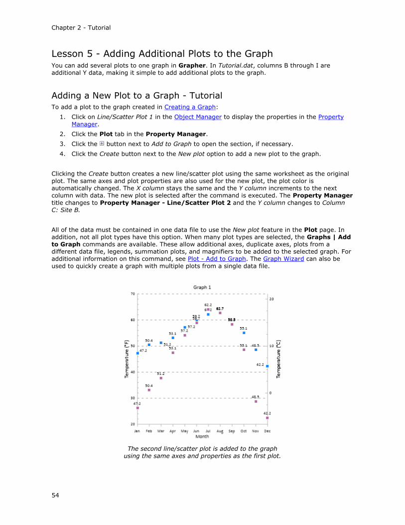
Chapter 2 - Tutorial
54
Lesson 5 - Adding Additional Plots to the Graph You can add several plots to one graph in Grapher. In Tutorial.dat, columns B through I are additional Y data, making it simple to add additional plots to the graph.
Adding a New Plot to a Graph - Tutorial
To add a plot to the graph created in Creating a Graph:
1. Click on Line/Scatter Plot 1 in the Object Manager to display the properties in the Property
Manager.
2. Click the Plot tab in the Property Manager.
3. Click the button next to Add to Graph to open the section, if necessary.
4. Click the Create button next to the New plot option to add a new plot to the graph.
Clicking the Create button creates a new line/scatter plot using the same worksheet as the original plot. The same axes and plot properties are also used for the new plot, the plot color is automatically changed. The X column stays the same and the Y column increments to the next column with data. The new plot is selected after the command is executed. The Property Manager
title changes to Property Manager - Line/Scatter Plot 2 and the Y column changes to Column C: Site B.
All of the data must be contained in one data file to use the New plot feature in the Plot page. In addition, not all plot types have this option. When many plot types are selected, the Graphs | Add to Graph commands are available. These allow additional axes, duplicate axes, plots from a different data file, legends, summation plots, and magnifiers to be added to the selected graph. For additional information on this command, see Plot - Add to Graph. The Graph Wizard can also be used to quickly create a graph with multiple plots from a single data file.
The second line/scatter plot is added to the graph using the same axes and properties as the first plot.

55
Changing the Plot Type - Tutorial
Let's change the new scatter plot into a line plot to help differentiate between the two curves. Previously, we changed from a line plot to a scatter plot by editing the Line and Symbol properties in the Property Manager. There is also a shortcut to changing between plot types.
To change the scatter plot into a line plot:
1. Click on the Line/Scatter Plot 2 in the Object Manager.
2. Click the Graph Tools | Convert | Plot Type | Line command. The scatter plot changes to a line plot.
3. Click on the Labels tab in the Property Manager.
4. To remove the labels, set the Label column property to None.
The Graph Tools | Convert | Plot Type command is not available for all plot types. It can be used to
convert line, scatter, line/scatter, step, and bar charts to other line, scatter, line/scatter, step, and
bar charts. The Graph Tools | Convert | Graph to 2D/3D command can be used to convert a 2D graph to a 3D graph, or vice versa, when the entire graph is selected.
You can change the properties in the new plot to distinguish it from the first plot.
Adding Semi-Transparent Fill - Tutorial
Adding a semi-transparent fill to the line plot will help distinguish it from the scatter plot. Color gradients can be used to enhance the appearance of the fill and can be mapped to specific values.
To add fill to the line plot:
1. Click on Line/Scatter Plot 2 in the Object Manager, if it is not already selected.
2. Click on the Fill tab in the Property Manager to display the fill properties.
3. If necessary click the next to Gradient to expand the gradient properties.
4. Change the gradient Type to Linear.

Chapter 2 - Tutorial
56
5. Click the button next to the Colormap selection to open the Color Gradient dialog.
6. In the Presets list, select the Blues preset.
7. In the Opacity field, highlight the current 100% value and type 40.
8. In the Maximum field, type 83.
9. Click OK in the Color Gradient dialog.
A gradient fill has been added to Line/Scatter Plot 2. The color gradient was mapped between the
overall minimum and maximum values in the data file, 22.5 (December at Site B) and 83 (July at Site D). Mapping the color gradient to specific values allows you to represent equal data values with the same color across multiple plots when the plots use the same color gradient.
Fill the line plot with semi-transparent yellow fill.
Lesson 6 - Editing Graph Properties Graph properties control settings that affect the entire graph, such as titles, background line and fill colors, and fill patterns that fill between multiple plots. Let’s edit the graph title and set the background fill and line properties for the graph.
Editing a Graph Title - Tutorial
To add a graph title:
1. Click on the Graph 1 object in the Object Manager to select the entire graph.
2. Click on the Title tab in the Property Manager.
3. In the Text property field, delete Graph 1 and type the graph title, Average Daily Maximum.
4. Click the button next to Font to open the section, if necessary.
5. Highlight the current Size (points) value and change it to 20.
The Text and Font properties can be used to quickly add and modify a simple text title. The Text Editor can be used to add multiple lines and various fonts, sizes, and colors to the title.

57
Add a graph title to display additional information about the graph.
Setting Background Fill and Line Properties - Tutorial
To set the background fill and line properties:
1. With the Graph 1 selected, click on the Fill tab in the Property Manager.
2. Click the next to Background Fill Properties to open the section, if necessary.
3. Set the Foreground color to 10% Black by clicking on the existing color and selecting the
10% Black color from the palette.
The graph now has a light gray background, and all axes and the graph are labeled.
Set graph properties by clicking on the Graph object to add a final finished appearance to a
graph.
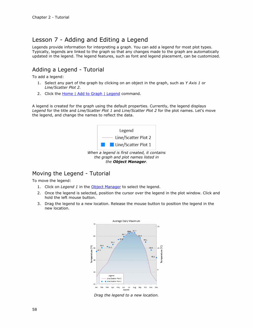
Chapter 2 - Tutorial
58
Lesson 7 - Adding and Editing a Legend Legends provide information for interpreting a graph. You can add a legend for most plot types. Typically, legends are linked to the graph so that any changes made to the graph are automatically updated in the legend. The legend features, such as font and legend placement, can be customized.
Adding a Legend - Tutorial
To add a legend:
1. Select any part of the graph by clicking on an object in the graph, such as Y Axis 1 or Line/Scatter Plot 2.
2. Click the Home | Add to Graph | Legend command.
A legend is created for the graph using the default properties. Currently, the legend displays Legend for the title and Line/Scatter Plot 1 and Line/Scatter Plot 2 for the plot names. Let's move the legend, and change the names to reflect the data.
When a legend is first created, it contains
the graph and plot names listed in the Object Manager.
Moving the Legend - Tutorial
To move the legend:
1. Click on Legend 1 in the Object Manager to select the legend.
2. Once the legend is selected, position the cursor over the legend in the plot window. Click and hold the left mouse button.
3. Drag the legend to a new location. Release the mouse button to position the legend in the new location.
Drag the legend to a new location.

59
Editing the Legend Title - Tutorial
To change the legend title:
1. Click on Legend 1 in the Object Manager to select the legend.
2. In the Property Manager, click on the Title tab.
3. Type the title Site Location Key in the Text property field and press ENTER.
Editing the Plot Names - Tutorial
To change the plot names in the legend:
1. Click on Legend 1 in the Object Manager to select the legend.
2. In the Property Manager, click on the Legend tab to open the legend properties.
3. Next to the Entries option, click the Edit button. This opens the Legend Entries dialog.
4. In the Legend Entries dialog, click Line/Scatter Plot 1 under the Name column.
5. Click the Rename button. This opens the Text Editor.
6. Let's change the text to Site A to match the worksheet. Highlight Line/Scatter Plot 1 and type Site A.
7. Click OK to close the Text Editor.
8. In the Legend Entries dialog, click Line/Scatter Plot 2 under the Name column.
9. Click the Rename button. This opens the Text Editor.
10. Another way to change the text is to link the text from a worksheet cell. Highlight the Line/Scatter Plot 2 text and press the DELETE key on your keyboard.
11. Click the button.
12. Select the Tutorial.dat file in the Open worksheets list, and click Open.
13. Click the button to open the Enter Cell dialog.
14. In the Enter Cell dialog, type C1 and click OK. The text <<@C1>> will be displayed in the Text Editor, indicating linked worksheet text.
15. Click OK in the Text Editor. The Line/Scatter Plot 2 is updated to Site B, as indicated in cell C1 of the specified worksheet. This text will automatically update if the text in cell C1 of the worksheet changes.
16. Click OK to close the Legend Entries dialog. The legend updates with the modified names.
The legend is updated with
the changes made in the Legend Entries dialog.
Changing the Number of Symbols - Tutorial
The number of symbols in a legend can be set from zero to three.

Chapter 2 - Tutorial
60
To change the number of symbols:
1. Click on Legend 1 in the Object Manager to select the legend.
2. In the Property Manager, click on the Legend tab to open the legend properties.
3. Click the number 2 next to the Number of symbols option and select 1 from the list. The
legend is updated displaying only one symbol.
Changing the Symbol Size - Tutorial
By default, legend entry symbols are the same size as the symbols in the plot. To change the symbol size to a custom value:
1. Click on Legend 1 in the Object Manager to select the legend.
2. In the Property Manager, click on the Legend tab.
3. Click the Edit button next to the Entries option to open the Legend Entries dialog.
4. Select the Site A in the Name column and click the Symbol Size button to open the Symbol Size dialog.
5. Select the Custom option in the Size group.
6. Type 0.25 in. (0.635 cm) in the Custom field.
7. Click OK in the Symbol Size dialog to make the change.
8. Click OK in the Legend Entries dialog.
The symbol size for Site A in the legend is now 0.25 inches. If the other plot also displayed symbols, checking the Apply to all entries option in the Symbol Size dialog would make all plots show the symbols at the specified size.
Changing the Line Length - Tutorial
In addition to changing the number and size of the symbols, the length of the displayed line can be changed.
To change the line length:
1. Click on the Legend 1 in the Object Manager to select the legend.
2. In the Property Manager, click on the Legend tab.
3. Highlight the value next to the Line length option. Type the new value of 0.500 in (1.270 cm) and press ENTER on the keyboard. The line next to Site B is lengthened to .5 inches.
Adding a Drop Shadow - Tutorial
To add a drop shadow behind the legend:
1. Click on the Legend 1 in the Object Manager to select the legend.
2. In the Property Manager, click on the Legend tab.
3. Click the button next to Frame to open the section, if necessary.
4. Check the box next to Display shadow to add a shadow behind the legend.
5. Click the color next to Shadow color to open the color palette and change the shadow color if desired.
The drop shadow is added to the legend.

61
Creating Multiple Columns in the Legend - Tutorial
Longer legends may need to be split into multiple columns to make the best use of the page space. To separate a legend into multiple columns:
1. Click on Legend 1 in the Object Manager to select the legend.
2. In the Property Manager, click the Legend tab.
3. Highlight the value next to the Number of columns option. Type the value 2, and press ENTER on the keyboard. The legend is updated to show the two columns.
All properties of the legend can be modified.
Lesson 8 - Working with the Script Recorder Scripter is Golden Software's automation program. You may record your actions in Grapher with the Script Recorder rather than writing the scripts manually in Scripter. See the Script Manager, Introducing Scripter, and Script Recorder help topics for more information about automation. The Grapher Automation book in the table of contents contains all of the help topics related to automation.
The Script Recorder can be used for many tasks. We will provide one scenario to demonstrate the Script Recorder. For example, let's say that you receive a data file once a quarter. The file has the same file name each quarter and the same number of columns, but the information contained in
the file updates each time. Each quarter you need to create the graphs and then export the graph
for reports. You can automate this process with the Script Recorder to save time and increase efficiency.
The graph in this example is fairly simple for time's sake, but keep in mind that complex graphs are very well suited to automation. We will record the process of creating some graphs, changing some features of a graph, saving the graphs, and exporting the graph. The creation of this graph uses the features included in the previous lessons and includes a few new items. If you do not understand part of the directions, review the material in the previous lessons or consult the online help.
Opening the Script Manager - Tutorial
The Script Manager can be used to view scripts as they record. Check the View | Display | Script
Manager command to display the Script Manager. A check mark is displayed next to visible managers. By default, the Script Manager is located at the right of the Grapher window, tabbed with the Worksheet Manager. Click the Script Manager tab to view the Script Manager. Right-
click in the Script Manager to access the menu commands.

Chapter 2 - Tutorial
62
Click the Script Manager tab to view, edit, and run scripts.
Start Recording - Tutorial
The Automation tab is used to start and stop recording scripts. Help for Grapher automation and Basic Language help information can also be accessed on the Automation tab.
To start recording, click the Automation | Scripts | Record command. The Record button changes
to Stop Recording to indicate that the script is recording. Information appears in the Script Manager as soon as recording begins. This code starts Grapher when the script is run later. Every action taken will be recorded in the script manager, until the recording is stopped.

63
Code is immediately added to the Script Manager when script recording begins. This information starts Grapher when the script is run later. The text in green with an apostrophe
prefix are comments.
Creating a Line Plot - Tutorial
To create a line plot in a new plot window:
1. Click the File | New | Plot command.
2. Click the Home | New Graph | Basic | Line Plot command.
3. The Open Worksheet dialog appears. Browse to Grapher's Samples folder. The location of this folder varies depending on where the software was installed. If the software was installed in the default folder, the path is C:\Program Files\Golden Software\Grapher 13\Samples.
4. Select the tutorial script recorder.xls file.
5. Click Open to create the default graph and line plot.
A line plot is created with the first two available columns using the default properties. Grapher can create graphs from data containing date/time information. In this example, column A contains
dates, so dates are plotted on the X axis.

Chapter 2 - Tutorial
64
The original graph is created with the default properties.
Changing the X Axis Date/Time Limits - Tutorial
The axis limits can use the default limits or can be changed to show only a portion of the graph. Limits can be based on numerical values or on date/time values. To change the X Axis limits using date/time values:
1. Click X Axis 1 in the Object Manager to select it.
2. In the Property Manager, click on the Axis tab to display the axis properties.
3. Click the to the left of the Limits section to expand the axis limits.
4. Click the next to the 12/18/2008 0:00:00 value next to Minimum date/time to open the
Select Date/Time dialog.
5. Change the date to 1/1/2009 and click OK.
6. Dates can also be edited directly in the Property Manager. Highlight the 3/28/2009 value next to Maximum date/time and type 4/1/2009 and press ENTER.
The X Axis limits now range from 1/1/2009 to 4/1/2009. Date/time values can be displayed in any format on axis and plot labels and in the worksheet. However, M/d/yyyy h:mm:ss format must be used when entering date/time values in the Property Manager.

65
The axis updates to the new date/time limits.
Changing the X Axis Date/Time Tick Mark Spacing - Tutorial
Tick marks can be spaced at any desired interval. Tick marks can be changed to show one tick mark every X number of units or can be based on date/time units, such as minutes, days, months, or years. To set the tick marks to display one tick and label per month:
1. Click on the X Axis 1 in the Object Manager to select it.
2. In the Property Manager, click on the Ticks tab to display the tick mark properties.
3. Click the to the left of the Major Ticks section to expand the major tick options, if
necessary.
4. Check the box next to the Use date/time spacing option.
5. Next to Date/time spacing, click Every Year to open the Date/Time Spacing dialog.
6. Change Year to Month and click OK.
The X Axis major tick marks are now displayed at 1/1/09, 2/1/09, 3/1/09, and 4/1/09.

Chapter 2 - Tutorial
66
The X Axis tick mark spacing can be based on date/time units.
Changing the X Axis Date/Time Tick Label Format - Tutorial
There are a variety of tick label formatting options available. One of the options is to change the display of the date/time labels. There are many different predefined date/time labels available or
you can create your own custom label format. To change the major label format from M/d/yy (1/1/2009) to MMM-yy (Jan-09):
1. Click on the X Axis 1 in the Object Manager to select it.
2. In the Property Manager, click on the Labels tab to display the tick label properties.
3. Click the to the left of the General section to expand the major label options, if necessary.
4. Click the Select button next to Major label date/time format to open the Date/Time Format Builder dialog.
5. Type MMM-yy in the Date/Time format (edit to change) field.
6. Click OK.
The X Axis tick labels are displayed in the MMM-yy format. The month abbreviations are determined
by your PC's default language setting. You can force a specific language for date/time labels by adding a language identifier before the date/time format.

67
The X Axis date/time labels can be formatted with a predefined or custom format.
Adding Linked Text to the Graph Title - Tutorial
Titles can be used to indicate the information contained in graphs. In this file, cell A1 contains the data's time range, January through March 2009. The next quarter's data file will contain April
through June 2009. With linked text, the information is updated on the graph any time the information changes in the cell in the data file. When the script is run, the date in the data file appears on the graphs.
To add linked text information to the graph title:
1. Select Graph 1 in the Object Manager.
2. Click the Title tab in the Property Manager to open the graph title properties.
3. Next to Text, click the button to open the Text Editor.
4. Delete the Graph 1 text in the Text Editor.
5. Click the button to select the worksheet that contains the text.
6. In the Open Worksheet dialog, select the tutorial script recorder.xls file from the Open worksheets section and click Open. The worksheet name is updated in the Text Editor.
7. Click the button in the Text Editor. Type A1 into the Enter Cell dialog and click OK. <<@A1>> appears in the Text Editor.
8. Highlight all of the text in the Text Editor. Change the size of the text to 24 by typing 24 in
the size box or clicking the next to the size box to change the size to 24. The font size box is located to the right of the font name.
9. Change any other properties, such as text color, if desired.
10. Click OK in the Text Editor to close the dialog and apply the changes.
Although we could add many more features to the graph, we will stop here. Feel free to experiment with adding or editing features and observing the script in the Script Manager.

Chapter 2 - Tutorial
68
Add the graph title with inserted text.
Exporting the Graph - Tutorial
Since the graphs are used to create a report, each graph must be exported for use in another program.
To export the graph:
1. Click the File | Export command or the button on the quick access toolbar.
2. Select a save location, such as your My Documents folder, in the Export dialog.
3. Type tutorial script recorder into the File name field in the Export dialog.
4. Select PDF (Vector) (*.pdf) from the Save as type list.
5. Check the Show options dialog option if it is not already selected. Selecting this option enables you to make any changes to the export options.
6. Clear the Use graph coordinates for export (when applicable) box. The Use graph coordinates for export (when applicable) exports the graph using graph coordinates. For reports and images, it is best to have this option unchecked.
7. Clear the Selected options only box. The Selected options only option only exports the items that are currently selected in the graph window.
8. Click the Save button.
9. In the Export Options dialog, click on the Vector PDF Options tab.
10. Click the Defaults button to return the export options to their default values.
11. Select the Embed fonts (when available) option to ensure the output PDF uses the same font as the graph.
12. Click OK and the PDF file is created.
Stopping and Saving the Script
Now that the graph has been created, it is time to stop recording and save the script. To stop and
save the script:

69
1. Click the Automation | Scripts | Stop Recording command. The Save As dialog appears.
2. Select a save location, such as your My Documents folder, in the Save As dialog.
3. Type tutorial script recorder into the File name box.
4. Click the Save button.
5. Right-click in the Script Manager and select File | Close to close the script in the Script Manager.
The recording is stopped and the tutorial script recorder.bas is saved for future use. Congratulations, you have completed the Grapher tutorial!
Advanced Tutorial - Using the Magnifier The Graph Tools | Add to Graph | Magnifier allows you to magnify a portion of a 2D graph.
To open a sample file and add a magnifier to a 2D graph:
1. Click the File | Open command.
2. Navigate to C:\Program Files\Golden Software\Grapher 13\Samples, select candlestick plot.grf and click Open.
3. Select Graph 2 in the Object Manager.
4. Click the Graph Tools | Add to Graph | Magnifier command or right-click on Graph 2 and select Add Magnifier.
5. The cursor changes to . Left-click and drag to define an area to magnify.
6. Release the cursor and the magnifier is created with the default settings. A Graph Magnfier 1
object is added to the Object Manager.

Chapter 2 - Tutorial
70
7. Select the Graph Magnifier 1 in the Object Manager.
8. In the Property Manager, click the Magnifier tab to display the magnifier properties. The
Selected box is Zoomed area box by default. The zoomed area box has six green boxes surrounding it in the plot window, indicating it is selected. Left-click the zoomed area box and drag it to a new location.
9. Drag the lower-right green box and drag the cursor to resize the zoomed area box.

71
10. In the Property Manager, click the Magnifier tab to display the magnifier properties.
Change the Selected box to Area selection box. The six green squares now surround the area selection box.
11. Drag a green square to resize the area selection box. The zoomed area box automatically
updates to reflect the changes made to the area selection size and location.

Chapter 2 - Tutorial
72
12. In the Property Manager, click the Tick Labels tab to display the tick labels properties.
The X Axis 1 is selected by default.
13. Click the next to Major Labels to expand the major label properties.
14. Click the check box next to Show labels to clear the box. The major label is removed.
15. Click the next to Minor Labels to expand the major label properties.
16. Check the box next to Show labels. The minor labels are displayed in the magnifier.
17. Click the next to Font to open the minor label font properties.
18. Change the Size (points) to 12.
19. Check the box next to Bold.
20. Click the next to Format to open the minor label format properties.
21. Click the Select button in the Date/time format field.
22. Type dd-MMM in the Date/Time format field of the Date/Time Format Builder dialog.
23. Click OK.
24. Next to Axes, click on X Axis 1 and select Y Axis 1 from the list.

73
25. In the Major Labels section, expand the Font section.
26. In the Font section, change the Size (points) to 18.
27. Check the box next to Bold.
28. In the Minor Labels section, check the Show labels box.
29. In the Font section, change the Size (points) to 14.
30. Check the box next to Bold.
You have now added a magnifier and adjusted various magnifier properties. To magnify a portion of
a 3D graph or polar plot, see the Using the Inset Zoom advanced tutorial lesson.
Advanced Tutorial - Using the Inset Zoom
The Insert | Inset Zoom command allows you to magnify a graph or any portion of the plot page. This type of inset is similar to changing the zoom level of the screen.
To open a sample file and draw an inset zoom:
1. Click the File | Open command.
2. Navigate to C:\Program Files\Golden Software\Grapher 13\Samples, select polar class scatter.grf and click Open.
3. Click the Insert | Inset Zoom command .
4. The cursor changes to . Left-click and drag to define an area to zoom in on.

Chapter 2 - Tutorial
74
5. Release the cursor and the inset zoom is created with the default settings. An Inset Zoom 1
object is added to the Object Manager.
6. Select the Inset Zoom 1. In the Property Manager, click the Magnifier tab to display the
magnifier properties. The Selected box is Zoomed area box by default. The zoomed area box

75
has six green boxes surrounding it in the plot window, indicating it is selected. Left-click the zoomed area box and drag it to a new location.
7. Drag the lower right green box and drag the cursor to resize the zoomed area box.
8. In the Property Manager, click the Lines tab to display the lines properties.
9. Click the to the left of Zoom Box to expand the zoom box section.
10. Click the to the left of Line to expand the line properties.
11. Next to Width, type 0.03 in and press ENTER.
12. Next to Color, click Black to open the color palette. Select Magenta. The color palette closes
and the lines update to the new color.
13. Next to Opacity, enter 50% and press ENTER.
14. In the Property Manager, click the Connector tab to display the connector properties.
15. Click the to the left of Fill style to expand the fill style properties.
16. Next to Foreground color, click 50% Black to open the color palette. Select Magenta. The
color palette closes and the lines update to the new color.
17. Next to Foreground opacity, enter 10% and press ENTER.

Chapter 2 - Tutorial
76
Advanced Tutorial - Combining Plots from Different Graphs In Grapher, a Graph is an object that contains the plots, axes, legends, summation plots, and other items used to display data as any of the plot types. Plots are the lines, symbols, or bars that display the data on the graph. Plots can be added to a graph with the Home | Add to Graph | Plot
command or can be moved between graphs in the Object Manager.
Adding a Plot to an Existing Graph
To add a plot to an existing graph:
1. Click on the existing plot, axis, or graph in the Object Manager to select it.
2. Click the Home | Add to Graph | Plot command.
3. Select the plot type and click OK.
4. Set the axes to use for the new plot, if required, and click OK.
5. Select the worksheet to use for the new plot, if required, and click Open.
6. The new plot is added to the existing graph.
Dragging a Plot from One Graph to Another
To drag a plot from one graph to another:
1. Click on a plot in the Object Manager.
2. Hold down the left mouse button and drag the plot to a different graph object.
3. Release the mouse button.
4. If multiple axes exist in the new graph, select the Graph, X Axis, and Y Axis in the dialog and click OK.
5. The plot is moved to the new graph and is drawn using the selected axes. The old graph still exists, but can be deleted if desired.

77
Copying a Plot from One Plot Window to Another
To copy a plot from one plot window to another:
1. Open a .GRF, .GPJ, or .GRT file.
2. Click on a plot in the Object Manager.
3. Click the Home | Clipboard | Copy command.
4. Open another .GRF, .GPJ, or .GRT file.
5. Click the Home | Clipboard | Paste command.
6. In the Choose Axes dialog, select the appropriate Graph, X Axis, and Y Axis. Click OK.
7. The plot is copied to the new plot window in the appropriate graph.
Notes:
Some plot types, such as radar plots and pie charts, cannot be moved between plots.
When more than one axis of any type exists on the graph, a dialog appears where you specify which axes to use.
2D plots can be moved to 3D plots, but the plot does not become a 3D plot. If you want to move a 2D plot to a 3D plot, first convert the 2D plot to a 3D plot using the Graph Tools | Convert | Graph to 2D/3D command . Then, drag and drop the 3D plot into the other 3D
graph.
A 3D plot can be moved to a 2D graph. The 3D plot becomes a 2D plot.
An XYZ plot can be moved to a 2D or 3D graph. If you drag a XYZ plot to a 2D graph, only two dimensions are displayed. If you drag a XYZ plot to a 3D graph, Grapher automatically
adds a new Z axis.
Congratulations! You have completed the Grapher advanced tutorial lessons.


79
Chapter 3 - Data Files and the Worksheet
Data files contain the information used to create a graph. Each record in a data file occupies a single row and is comprised of at least two values (X, Y) for most plot types and at least three values for XYZ plots, contour maps, and surface maps (X, Y, Z). At least three values are also
required for class plots, floating bar, hi-low-close, bubble, ternary, vector. The X, Y, and Z values are each placed in separate columns. X and Y coordinates define the position of the point on the graph.
Creating Data Data files can be created in the Grapher worksheet, an ASCII editor, or any program that can produce files in one of the file formats listed in the Open dialog.
Graphing and Viewing Data When graphing a data file, the data are loaded into an internal worksheet. It is not necessary to open the data in a worksheet window before creating a graph. If you want to view or alter the data
in a data file, you can use the File | Open, Graph Tools | Worksheet | Display, or View | Display | Worksheet Manager commands to gain access to the data.
The order of the data in the file is the order the data are plotted. Descriptive headers in row 1 of each column are helpful but not required. When text appears in row 1 of a column, this text appears in list boxes as column titles. If a number resides in row 1, it is not incorporated into the list boxes, and instead, the column heading (such as column B) is displayed.
Rows with non-numeric entries (empty cells or text) are excluded when graphing. These records are not considered during the graphing operation.
Data File Content Data files can contain up to one billion columns. Since you can specify the columns to be graphed, your data can occupy any columns. This allows you to have columns containing additional
information particular to each point. The data file can contain several columns, so you can produce several graphs using the same data file.
Data files may contain data in addition to the X, Y coordinates. For example, when creating a scatter graph with the Home | New Graph |Basic | Scatter Plot command, additional columns can be used to specify the plot labels and axis labels.
Data File Formats Import and export worksheet data in several data file formats.
Use File | Import to import the following formats into the worksheet:
ACCDB Microsoft Access 2007-2010
BLN Golden Software BLN Files
BNA Atlas BNA Files
CSV Comma Separated Variable CSV Files
DAT Files
DBF Database Files
MDB Microsoft Access 1997-2003 Files
SEG Data Exchange Format

Chapter 3 - Data Files and the Worksheet
80
P1 Data Exchange Format
SLK Sylk Spreadsheet Files
TXT Text Data Files
XLS Excel Files
XLSX Excel Files
XLSM Excel Files
Use File | Open Excel to import Excel files into a native Excel window.
XLS, XLSX, XLSM Excel Files
Use File | Save As to export the following formats from the worksheet:
BLN Golden Software BLN Files
BNA Atlas BNA Files
CSV Comma Separated Variable CSV Files
DAT Files
SLK Sylk Spreadsheet Files
TXT Text Data Files
XLS Excel Files
XLSX Excel Files
Date/Time Formatting In addition to numbers and text, dates and times are format types in Grapher. Dates and times can be used to create a graph, as axis and plot labels, to clip the graph, and to set axis limits.
Using Date/Time Formatting
To use dates and times in Grapher, the data need to be formatted as dates and times. One way to
format data in Grapher is to use the worksheet. The worksheet can be accessed with the File | New | Worksheet, File | Open, Graph Tools | Worksheet | Display, and through the Worksheet Manager. Highlight the column containing dates and times and then select Data Tools | Format | Format Cells to set the column as date/time in the worksheet.
Once the formatting is set to date/time, you can use the date/time information just as you would use numbers in Grapher:
you can plot the data using date/time without converting the dates and times into serial numbers
you can set the axis limits using dates and times
you can set plot clipping using dates and times
Date/time information can also be used as plot labels and tick labels.
Date/Time Formatting Tips
In the worksheet, save data files containing date/time formatting as Excel files to preserve the date time formatting as seen in the worksheet.
You can save date/time-formatted data files as ASCII files (.DAT, .CSV, .TXT, .BNA, or BLN). Sometimes this is necessary if you exceed the Excel row or column limits. When opening the

81
file in Grapher's worksheet, you can make the serial numbers appear as dates by using Data Tools | Format | Format Cells.
If you have formatted the data as date/time in another spreadsheet program such as Excel, the data are formatted as date/time in Grapher.
Whenever possible, enter and display dates and times in one of the many calendar formats, e.g., "6/14/2009” or “14-June-2009”, and let the software handle converting to/from internal numeric representations.
When the recognized format is ambiguous (i.e. 10/7/12), the month, day, and year order is determined by the Windows locale. In some countries, this will be recognized as M/d/yy, in others as d/M/yy, and in others as YY/M/d. It is important to use non-ambiguous date/time
formats when the Windows locale may change.
If dates/times occur before 1/1/0000, use the BC or BCE suffix after the date. So, Alexander
III of Macedon's birthday would be listed as 20-July-356 BCE in the worksheet. Using AD or CE is not necessary and the worksheet will automatically remove these in dates after
1/1/0000.
The year 0 is defined, according to the ISO 8601:2004 standard.
When a two digit year is input in the worksheet (00 to 99), it means the year in the current
century. For instance, inputting 11/4/13, indicates that the year is 2013, not 0013. In order to have the year 0013, the full four digits (0013) must be input for the date. So, the date would be input as 11/4/0013 CE for November 4, 0013 CE or 11/4/0013 BCE for November 4, 0013 BCE.
If the data is not displaying like you have specified in the Label Format dialog, check the Use Data/Time Format box in the Major Label Text section of the axes properties Tick Labels page.
When inputting date/time values in the Property Manager, date/times must always be entered as MM/dd/yyyy hh:mm:ss. No other formats are permitted in the date/time edit
boxes in the Property Manager.
Date Time Formats
Date and time formats can be set from the worksheet and from many locations in Grapher. Date and time options are case sensitive. Months always need to be entered with upper case M and minutes must always be entered with lower case m.
When dates are parsed during input/import, the month and day of week names must match those of the local language as set in the Windows Control Panel, otherwise the entry will not be
recognized as a valid date and will be treated as a text string.
When the recognized format is ambiguous (i.e. 10/7/12), the month, day, and year order is determined by the Windows locale. In some countries, this will be recognized as M/d/yy, in others as d/M/yy, and in others as YY/M/d. It is important to use non-ambiguous date/time formats when
the Windows locale may change.
General Date/Time Formats
These are the general date and time formats. These can be used in the worksheet Format Cells dialog, in the plot window label format section, or from the Date/Time Format Builder dialog. Any combination of these formats can be used in any of these locations.
Skip to the Predefined Date/Time Formats section for the allowed linked text formats.

Chapter 3 - Data Files and the Worksheet
82
All rows below use the date July 9, 2014 at 6:45:44.12345 in the evening for the Example.
Date/Time Code Example Description
d 9 Single digit day, excluding leading zero
dd 09 Double digit day, including leading zero
ddd Wed Shortened day of week name
dddd Wednesday Full day of week name
M 7 Single digit month, excluding leading zero
MM 07 Double digit month, including leading zero
MMM Jul Shortened month name
MMMM July Full month name
MMMMM J First letter of month name
yy 98 Two digit year
yyyy 1998 Full year
g Before Common Era designator - Includes space and bce or nothing if ce, lower case
gg ad BC/AD designator - Includes space and bc or ad, lower case
ggg ce Before Common Era designator - Includes space and bce or ce, lower case
G Before Common Era designator - Includes space and BCE or nothing if CE, upper case
GG AD BC/AD designator - Includes space and BC or AD, upper case
GGG CE Before Common Era designator - Includes space and BCE or CE, upper case
h 6 Single digit hours - 1-12, excluding leading zero
hh 06 Double digit hours - 01-12, including
leading zero
H 18 Hours - 0-23 military, excluding leading zero
HH 18 Hours - 00-23 military, including leading zero
[h] 1003914 Hours portion of total time, excludes leading zeros
m 45 Minutes - 0-60, excluding leading zero
mm 45 Minutes - 00 to 60, including leading zero
[mm] 45 Minutes portion of total time, includes leading zeros

83
ss 44 Seconds - 0-60, rounded to the nearest second
ss.0 44.1 Seconds - 0-60, rounded to the nearest
tenth of a second
ss.00 44.12 Seconds - 0-60, rounded to the nearest hundredth of a second
ss.000 44.123 Seconds - 0-60, rounded to the nearest millisecond
ss.0000 44.12345 Seconds - 0-60, maximum precision
[ss] 44 Seconds portion of total time, includes leading zeros
tt pm am or pm designator, lower case
TT PM AM or PM designator, upper case
\ escape character - output next character
verbatim
'...' output ALL characters between single quotes verbatim, including escape character
[$-xxxx] [$-409] xxxx is an up to four hex digit representation of a locale ID
Predefined Date/Time Formats
The predefined date/time formats are the only formats that can be used inside the linked text
brackets <<date/time>> when creating linked text via typing in the Text Editor or automation. You
can combine predefined formats by writing separate <<date/time>> fields in the Text Editor or script. For example, you can type <<M/d/yy>> <<h:mm TT>> in the Text Editor to display both time and date.
If you cannot create the desired format by combining predefined date/time formats, consider using the Insert Date/Time button in the Text Editor.
All rows below use the date July 9, 2014 at 6:45:44.12345 in the evening for the Example.
Date/Time Code Example Description
M/d/yy 7/9/14 Single digit month, Single digit day, two digit year - separated by forward slash
MM/dd/yy 07/09/14 Two digit month, day, and year - separated with forward slash
MMM dd, yyyy Jul 09, 2014 Shortened month name, two digit day, four digit year - separated by spaces and a comma
MMMM dd, yyyy July 09, 2014 Full month name, two digit day, four digit year - separated by spaces and a comma
d-MMM-yy 9-Jul-14 Single digit day, shortened month name,
two digit year - separated by hyphens

Chapter 3 - Data Files and the Worksheet
84
d-MMM 9-Jul Single digit day, shortened month name - separated by hyphens
MMM-yy Jul-14 Shortened month name, two digit year - separated by hyphen
MMM-yyyy Jul-2014 Shortened month name, four digit year - separated by hyphen
MMMM-yyyy July-2014 Full month name, four digit year - separated by hyphen
h:mm TT 6:45 PM clock Hours and minutes with AM/PM designator
h:mm:ss TT 6:45:44 PM Hours, minutes, and seconds with AM/PM
designator
HH:mm 18:45 24-hour clock hours and minutes
HH:mm:ss 18:45:44 24-hour clock hours, minutes, and seconds
M/d/yy HH:mm 7/9/14 18:45 Single digit month, single digit day, two digit year, 24-hour clock hours and
minutes
yyyy 2014 Four digit year
yy 14 Two digit year
MMMM July Full month name
MMM Jul Shortened month name
MM 07 Two digit month
M 7 Single digit month
dddd Wednesday Full day name
ddd Wed Shortened day name
dd 09 Two digit day
d 9 Single digit day
d/M/yy 9/7/14 Single digit day, single digit month, two digit year - separated by forward slash
dd/MM/yy 09/07/14 Two digit day, two digit month, two digit year - separated by forward slash
yy/MM/dd 14/07/09 Two digit year, two digit month, two digit day - separated by forward slash
yyyy-MM-dd 2014-07-09 Four digit year, two digit month, two digit day - separated by hyphen
Date/Time Format Builder Dialog
In the Text Editor dialog, click the button to open the Date/Time Format Builder dialog.
From the worksheet, click the button in the Format Cells dialog Number page. The Date/Time
Format Builder dialog is also accessed by clicking the Select button in the Date/time format field in the Label Format section of the Property Manager and clicking a format in the Date/Time

85
Labels dialog. When the Date/Time Format Builder is used to insert date/time math text instruction with the Text Editor, the date/time will update every time the project updates.
The Date/Time Format Builder dialog is used to insert or create date/time formats for worksheet cells or text objects.
Date/Time Format
Type a Date/Time Format into the Date/Time format (edit to change) field to set the date/time format. You can also use the Language (Country) and Predefined date/time formats lists to insert multiple date/time formats and languages.
Language (Country)
By default, the program will use the computer's default language settings for displaying the date/time options in the worksheet. The computer default is controlled by the Windows Control Panel. Refer to your Windows documentation for information about setting the locale. The Language
(Country) uses the same codes to override the display. For instance, if the date/time values should always be displayed in English, regardless of locale, you could select English (United States) - [$-409] and click the Insert button. Insert the locale setting first in the Date/Time format box. Any cells with the specified language will appear in that language. In addition, the options in the Predefined date/time formats will change to show the common formats for that locale. Locale IDs are input as [$-####] in the Date/Time format field, where the #### is the locale identifier.
Note: The Insert button must be clicked after selecting the Language (Country) option. Simply selecting the Language (Country) does not change the Date/Time format. The Date/Time format
does not change until Insert is clicked.
Predefined Date/Time Formats
The Predefined date/time formats list contains the common formats for the selected Language (Country) option or for your Windows locale. Available formats are made of combinations of year,
month, day, hours, minutes, seconds, and AM/PM designation. Years are shown as yy or yyyy. Months are shown as M, MM, MMM, MMMM, or MMMMM. Days are shown as d, dd, ddd, or dddd. Hours are shown as h, hh, H, HH, or [h]. Minutes are shown as m, mm, or [mm]. Seconds are shown as ss, ss.0, ss.00, ss.000, ss.0000, or [ss]. AM/PM designation is shown as tt or TT. BC/AD designation is shown as gg or GG. BCE/CE designation is shown as g, G, ggg, or GGG. Refer to formats for information about each specific option.

Chapter 3 - Data Files and the Worksheet
86
Note: The Insert button must be clicked after selecting the Predefined date/time formats option. Simply selecting the Predefined date/time formats does not change the Date/Time format. The Date/Time format does not change until Insert is clicked.
Sample
The Sample text updates to show a sample of the current entry in the Date/Time format (edit to change) field.
Data in the Plot In the plot window, there are several ways to ascertain the data used in the plot and to update the data.
Click the Graph Tools | Worksheet | Display command to open the data used to create the graph. The data opens in the Grapher worksheet. You need to select a single plot to activate
the command. If any other objects are selected, e.g., entire graphs, axes, titles, drawing objects, the Display command is not available.
Click Graph Tools | Worksheet | List to view the path and file names of all the data files used
in the current Grapher document.
Use the Auto Track Worksheets option on the Plots page of the File | Options dialog to
automatically show changes in the Grapher worksheet on the graph. If Auto Track Worksheets is disabled, changes made to the worksheet do not show on the graph. Note that this command only applies to changes made in the Grapher worksheet.
The File | Reload Data command is used to apply changes to a graph when changes to the data are made in programs other than Grapher. For example, if you have a data file open in Excel and make changes to the data file, you can use File | Reload Data to display the changes in the graph.
List Worksheets Click the Graph Tools | Worksheet | List command to view the path and file names of all the data files used in the current Grapher document.
Display Worksheet Click the Graph Tools | Worksheet | Display command to open the data used to create the graph. The data opens in the Grapher worksheet. You need to select a single plot to activate the command. If any other objects are selected, e.g., entire graphs, axes, titles, drawing objects, the
Display command is not available.
Auto Track Worksheets Use the Auto track worksheets option to automatically show changes in the Grapher worksheet on the graph. To enable or disable Auto track worksheets, click the File | Options command. On the left side of the dialog, click on Plots. On the right side of the dialog, check or uncheck the box next to Auto track worksheets.
If Auto track worksheets is disabled, changes made to the worksheet do not show on the graph. This command only applies to changes made in the Grapher worksheet. If changes are made in a program other than Grapher, use the File | Reload Data command to update the data.

87
Reload Worksheets The File | Reload Data or Graph Tools | Worksheet | Reload command is used to apply changes to a graph when changes to the data are made in programs other than Grapher. For example, if you have a data file open in Excel and make changes to the data file, you can use the
Graph Tools | Worksheet | Reload command to display the changes in the graph.
To show changes in a graph when data is edited in another program:
1. Make changes to the data in a program other than Grapher.
2. Save the changes in the other program. If you do not save the changes, they will not appear in the graph.
3. Click the File | Reload Data or Graph Tools | Worksheet | Reload command.
If you are editing your data in the Grapher worksheet, use Auto Track Worksheets, not Reload. If
you make changes in the Grapher worksheet and do not save the changes, using the Graphs | Worksheet | Reload command removes the data changes.
Change Worksheets Click the Graph Tools | Worksheet | Change command to change the paths for all worksheet references in the current plot document. The Change command updates the Worksheet property for ALL plots in the document to the selected folder. The Change command does not affect the file name.
The Change command cannot be undone with the Undo command. If the incorrect path is selected
in the Select Folder dialog, use the Change command again to select the desired path. Alternatively, you can close the document without saving and reopen the document.
To change the worksheet paths:
1. Click the Graph Tools | Worksheet | Change command.
2. Select the desired location in the Select Folder dialog
3. Click Select Folder in the Select Folder dialog.
The Worksheet property in the Plot page of the Property Manager will be updated for all plots in the document to the new path.
New Path Contains Data
When the new path contains files with the same file name as the old path, the plots will be automatically updated with the data in the new location.
New Path Does Not Contain Data
When the new path does not contain files with the same file name as the old path, the plots will be unchanged as long as the document is open in Grapher. However, once the document is saved, closed, and reopened you will be prompted to update the file paths if the data files are not in the specified path.

Chapter 3 - Data Files and the Worksheet
88
Worksheet Window The worksheet window contains commands to display, edit, enter, and save data. The worksheet window has several useful and powerful editing, transformation, and statistical operations available. Several import and export options are available for opening data files from other spreadsheet
programs. The Data Tools tab is automatically selected when you open or switch to a worksheet document.
Worksheet Commands
Some commands are not available when viewing a worksheet. For example, none of the Insert and Layout commands are available and only a few of the Home and View commands are available.
File Opens, closes, saves, imports, exports, and prints files. Provides links to online references and email templates. Provides access to licensing information and
Grapher version number.
Home Contains clipboard, undo, and graph creation commands.
View
Controls the display of toolbars, managers, status bar, tabbed documents, and the window layout.
Automation Contains links to record or run a script and open the automation or BASIC language help files.
Data Tools Contains commands for modifying the worksheet appearance, editing the data file, and analyzing the data.
The Application/Document Control menu commands control the size and position of the application window or the document window.
Worksheet Window
To enter data in a worksheet, use the File | Open command to open an existing data file or click the File | New | Worksheet command to create a blank worksheet. Data already used to create plots can be opened in the worksheet window with the Graph Tools | Worksheet | Display command.
The components of the worksheet window are discussed below.
The components of a worksheet window shown above are described in the following table.
Column Letters The column letters identify a column in the worksheet.

89
Row Numbers The row numbers identify a row in the worksheet.
Active Cell
The active cell is highlighted with a bold outline. The active cell receives
data input (numeric values or text strings) from the keyboard. Only one cell is active at a time.
Active Cell Location
The active cell location is specified by column letter and row number.
Active Cell Edit Box
The active cell edit box displays the contents of the active cell. Data
typed into an empty cell appears in both the edit box and the active cell.
Worksheet Name The worksheet name displays the data file name or the worksheet number if the data file has not been saved.
Select Entire Worksheet Button
The select entire worksheet button is used to select all cells in the worksheet.
Opening a Worksheet Window
You can view, enter, or modify data in the worksheet document.
To view worksheet data:
Click the File | New | Worksheet command to open a new blank worksheet.
Click the button to open a new blank worksheet.
Click the File | Open command. In the Open dialog, select a data set, and click the Open
button.
If there is an open worksheet window, return to it at any time by clicking on the tab with
that worksheet name displayed.
Open Excel
The File | Open Excel command opens an .XLS, .XLSX, or .XLSM file using Excel. All commands and features of Excel are available in Grapher when using this command. You can easily create graphs from the Excel window using the New Graph menu commands. The Excel window New Graph menu commands are the same as the Grapher Home | New Graph commands.
An Excel file opened with the File | Open Excel command cannot be saved to the same file name. Excel locks the file so that it can only be saved in the open Excel window using the File | Save As command. This is an Excel limitation. To save the changes, choose the File | Save As command and save the Excel file to a new file name.
Note: With older .XLS files and the 64-bit version of Grapher, the File | Open Excel command will
sometimes open the file directly in Excel, not in the Grapher window. This is because Excel is opening the file in a compatibility mode not supported by Excel's automation interface. The file can be opened in Excel and saved to a newer format to be able to edit the file in Grapher.
Working with Worksheet Data There are three ways to enter data into the worksheet. Data are entered into the worksheet using File | Open to open a data file, typing data directly into the worksheet, or copying the data from another application and pasting it into the worksheet.

Chapter 3 - Data Files and the Worksheet
90
Entering Data into a Cell
Edit the contents of a cell by making it the active cell. The active cell is positioned by clicking on a cell with the mouse, by using the ARROW keys, PAGE UP, PAGE DOWN, TAB, HOME, END, and SHIFT+TAB. Press the F2 key or highlight the contents of the active cell edit box to edit the contents of the cell.
To enter new data and delete the old, position the active cell and begin typing. Edit mode is entered
automatically and the old data is deleted. Pressing ENTER, Up or Down ARROWS, TAB, SHIFT+TAB, PAGE UP, or PAGE DOWN keys cause the edit changes to be recorded permanently in the cell. After pressing F2 or highlighting the cell edit box use the HOME, END, BACKSPACE, DEL, and ARROW keys to edit the cell. Pressing ESC while editing a cell cancels the changes and restores the original data.
Moving the Active Cell
You can designate any worksheet cell as the active cell by left-clicking on it with the mouse. The active cell can also be repositioned by using keyboard commands. The active cell is the cell with a thick border drawn around it. The following actions can be used to move the active cell:
ARROW keys (Up, Down, Left, Right) move the active cell to an adjacent cell.
PAGE UP/PAGE DOWN moves the active cell up or down by the number of rows visible in the
window.
HOME moves the active cell to the first occupied cell in the current column. Pressing HOME
again moves the active cell to the top row in the current column.
END moves the active cell to the last occupied row in the current column. Pressing END again
moves the active cell to the bottom row of the worksheet.
ENTER moves the active cell down one row and ends "edit mode."
TAB moves the active cell right one column and ends "edit mode."
SHIFT+ENTER moves the active cell up one row and ends "edit mode."
SHIFT+TAB moves the active cell left one column and ends "edit mode."
CTRL+HOME moves the active cell to the top cell of the left most column in the worksheet (A1).
CTRL+END moves the active cell to the bottom occupied row of the last occupied column in the worksheet.
The CTRL+LEFT ARROW behavior depends on the position of the active cell. If the active cell is to the right of the last occupied column in the current row, it moves the active cell to the last occupied column in the current row. If the active cell is in or to the left of the last
occupied column in the current row, but to the right of the first occupied column in the current row, it moves the active cell to the first occupied column in the current row. Otherwise, CTRL+LEFT ARROW moves the active cell to the first column in the current row.
The CTRL+RIGHT ARROW behavior depends on the position of the active cell. If the active
cell is to the left of the first occupied column in the current row, it moves the active cell to the first occupied column in the current row. If the active cell is in or to the right of the first occupied column in the current row, but to the left of the last occupied column in the current row, it moves the active cell to the last occupied column. Otherwise, CTRL+RIGHT ARROW moves the active cell to the last column in the current row.
The CTRL+UP ARROW behavior depends on the position of the active cell. If the active cell is below the bottom occupied row in the current column, it moves the active cell to the bottom
occupied row in the current column. If the active cell is below the top occupied row in the current column, but in or above the bottom occupied row in the current column, it moves the

91
active cell to the top occupied row in the current column. Otherwise, CTRL+UP ARROW moves the active cell to the first row in the current column.
The CTRL+DOWN ARROW behavior depends on the position of the active cell. If the active cell is above the top occupied row in the current column, it moves the active cell to the top occupied row in the current column. If the active cell is above the bottom occupied row in the current column, but below the top occupied row in the current column, it moves the active
cell to the bottom occupied row in the current column. Otherwise, CTRL+DOWN ARROW moves the active cell to the last row in the current column.
Moving the Active Cell within Selections
The ENTER, TAB, SHIFT+ENTER, and SHIFT+TAB keys move the active cell within a group of selected cells without canceling the selection.
Pasting Data
If data are copied to the clipboard from another software application, the contents of the clipboard can be pasted into the worksheet. If the source application is Microsoft Excel, some formatting information is retained. When pasting data into the worksheet, select a cell and use Home | Clipboard | Paste (CTRL+V). Any data to the right or below the active cell is overwritten, so be sure to locate the active cell carefully. When data are copied to the clipboard, special formatting
information is also copied. The Home | Clipboard | Paste | Paste Special command determines the format in which the contents are pasted into the worksheet.
Data Tools Tab
Use the commands on the Data Tools tab to edit, search, format, sort, view statistics, transform the data using mathematical functions, or transpose the data.
Worksheet Error Codes and Special Numeric Values
There are a few different error codes and special numeric values that can appear in a worksheet cell depending on the type and nature of the data that appears.
Codes Explanation
######### number does not fit in the column, i.e., the column must be wider for the number to be shown
#N/A value cannot be computed, e.g., not enough data to calculate a statistic
#DIV/0! an attempt to divide-by-zero was made in performing a calculation
#ERROR a value could not be computed, e.g., square root of a negative number
#OVERFLOW value is too large for the worksheet (largest absolute value is about 1.797E+308)
1.#INF value is too large for the worksheet, i.e., "infinite" value surpassed
1.#IND numeric value is indefinite (usually the result of performing a calculation with an infinite value or attempting to divide by zero)
Selecting Cells
The keyboard and the mouse may be used to select cells. Selected cells are indicated by reverse video (white background becomes black, etc.). Hidden cells are selected if their columns or rows

Chapter 3 - Data Files and the Worksheet
92
are within a selected block of cells. Single cells, a rectangular block of cells, one or more rows, one or more columns, or the entire worksheet can be selected.
Cells may be selected to:
Perform editing and clipboard functions.
Compute statistics for selected cells.
Set cell properties for several cells via the Data Tools tab, such as column width, row height,
and cell format.
There are several ways to select cells:
Clicking on the small box above the row labels and to the left of the column label bar selects
the entire worksheet.
To deselect all selected cells, click the left mouse button anywhere within the worksheet, or
move the active cell with an ARROW key or other movement key.
To rapidly select a large block, first select one corner of the block, and then use the scroll
bars to scroll to the opposite corner. Hold down the SHIFT key and click on the cell at the opposite corner. The PAGE UP, PAGE DOWN, HOME, and END keys may also be used, but the SHIFT key must be held down while these keys are pressed. The SHIFT key is not needed while using the scroll bars.
To select all cells in a column or row, click the column letter or row number. To select several adjacent columns or rows, press and hold the left mouse button and drag the pointer on the column letters or row numbers. To deselect a single row or column from a multiple row or column selection, hold CTRL and click the row or column label.
While holding down the CTRL key, the active cell may be repositioned for selecting a new
block.
The CTRL key is used to select multiple blocks and the SHIFT key is used to resize the last
selected block. Details and exceptions are given in separate help sections for selecting with
the mouse and selecting with the keyboard.
If entire rows or columns are selected by clicking on the headers, some operations, such as statistics, can take a long time. Rather than clicking on the headers, only select the cells containing data.
Clicking and holding the left mouse button while dragging the mouse in the worksheet selects a block. Similarly, using the SHIFT key plus the ARROW keys selects a block.
The keys used with SHIFT for selecting cells are the ARROW keys, PAGE UP, PAGE DOWN, HOME, and END. TAB and SHIFT+TAB cannot be used.
While holding down the SHIFT key, the last selected block may be resized. Use the SHIFT key and the mouse or the SHIFT key and ARROW keys.
The active cell is at one corner (or edge) of a selected block and must first be positioned before selecting multiple cells.
The last block cannot be resized if the active cell has been moved.
Selecting Cells with the Keyboard
The keyboard may be used to select cells. Selected cells are indicated by reverse video (white background becomes black, etc.).

93
To Select Process
Single cells Click in the cell to select it, or use the arrow keys to select a cell. The selected cell has a thick outline around it.
A rectangular block of cells
Move the active cell to one corner of the block. While holding down the SHIFT key, use the movement keys to position the
opposite corner of the block. The movement keys include the ARROW keys, PAGE UP, PAGE DOWN, HOME, and END, but not TAB and SHIFT+TAB. When the block has been sized, release the SHIFT key. To resize the block, see the instructions below.
Several adjacent rows Select the first or last row. Then, while holding down the SHIFT
key, use the vertical movement keys. These include up ARROW, down ARROW, PAGE UP, PAGE DOWN, HOME, and END.
Several adjacent columns Select the first or last column. Then, while holding down the SHIFT key, use the right and left ARROW keys.
Resize Last Selected Block
To resize the last selected block, hold down the SHIFT key while using the movement keys (as appropriate to the type of block). The last block cannot be resized if the active cell has been moved.
Deselect All Selected Cells
To deselect all selected cells, click the left mouse button anywhere within the worksheet or move the active cell with an ARROW key or other movement key.
Selecting Cells with the Mouse
The mouse may be used to select cells. Selected cells are indicated by reverse video (white background becomes black, etc.).
To Select Process
Single cells Click on the cell with the left mouse button. The selected cell has a thick outline around it.
A rectangular block of cells Move the active cell to one corner of the block. Click and hold the left mouse button, and drag it to the opposite corner of the block. Then release the mouse button.
An entire row Click the mouse on the row label.
Several adjacent rows Click and hold the mouse on the first row label and drag it
to the last row. Make sure the cursor is a normal cursor not the double arrow cursor used for selecting row dividing lines. Hold CTRL and click a row label to deselect the row while keeping the other rows selected.
An entire column Click the mouse on the column label.
Several adjacent columns Click and hold the mouse on the first column label and drag it to the last column. Make sure the cursor is a normal
cursor not the double arrow cursor used for selecting column dividing lines. Hold CTRL and click a column label

Chapter 3 - Data Files and the Worksheet
94
to deselect the column while keeping the other columns selected.
The entire worksheet Click on the small box above the row labels and to the left of the column label bar.
The worksheet scrolls automatically if the mouse is dragged past the visible limits of the worksheet.
Select Additional Blocks
To select additional blocks, hold down the CTRL key while clicking.
Resize the Last Selected Block
To resize the last selected block, hold down the SHIFT key while clicking and holding the left mouse
button. Then, drag the edge of the last selected block to the new position. The last block cannot be resized if the active cell has been moved.
Deselect All Selected Cells
To deselect all selected cells, click the left mouse button anywhere within the worksheet or move the active cell with an arrow key or other movement key.
Row and Column Label Bars
The worksheet cells are located by column label bars (A, B, C…) or row label bars (1,2,3…). Click the label to select entire rows or columns, to change row height, to change column width, or to hide or unhide rows and columns. To select multiple rows or columns, drag the mouse over several adjacent labels.
This example shows columns A, B, C, and D, and rows 1, 2, 3, and 4.
Selecting a Column or Row Dividing Line
The column or row dividing lines are the lines between the column letter labels and row number labels along the borders of the worksheet. These lines divide the columns or rows. When selecting a dividing line, the cursor must be within approximately a character's width of the dividing line and it must be on the label bar.
You can change the column width or row height by dragging the dividing line. Rows or columns can be hidden or unhidden by using the mouse. The Column Width or Row Height commands can also be used to set column widths or row heights.

95
This example shows the cursor
being used to change the
width of column A.
This example shows the cursor
being used to change the height of row 3.
Worksheet Technical Specifications
The following technical specifications for the worksheet include the number of cells allowed in the worksheet and the nature of the numbers allowed in the worksheet.
Maximum number of rows in a worksheet: 1 billion
Maximum number of columns in a worksheet: 1 billion
Approximate memory requirements (for unformatted numeric data): 10.5 bytes per cell + 24 bytes per column
Maximum numeric precision (counting the digits before and after the decimal place): 15 digits
Maximum numeric resolution (the smallest detectable difference between two numbers): 2.22E-16
Maximum absolute value (the largest value that can be represented): 1.79769E+308
Minimum absolute value (the smallest value that is different from zero): 2.22507E-308

Chapter 3 - Data Files and the Worksheet
96
Example 1
This example has 10,000 rows of numbers in three columns.
30,000 cells x 10.5 bytes/cell = 315,000 bytes (308 Kbytes)
3 columns x 24 bytes/column = 72 bytes
TOTAL MEMORY NEEDED (in addition to memory needed to run the program): 380 Kbytes
Example 2
This example has three rows of numbers in 10,000 columns.
30,000 cells x 10.5 bytes/cell = 315,000 bytes (308 Kbytes)
10,000 columns x 24 bytes/column = 240,000 bytes (234 Kbytes)
TOTAL MEMORY NEEDED (in addition to memory needed to run the program): 542 Kbytes
Active Cell Functions
Enter or edit data in the active cell. The contents of the active cell are displayed in the active cell edit box. To edit existing data, activate the desired cell and press the F2 key or highlight the information in the active cell edit box.
Special key functions when editing the active cell are:
ENTER stores the contents of the cell edit box and then moves the active cell down one cell.
CTRL+ENTER completes the entry and keeps the current cell active.
Left and right ARROWS move within the cell's text if the F2 key has been pressed. Otherwise,
these keys store the contents of the cell edit box and then move the active cell to the left or right.
DELETE deletes the character to the right of the cursor if the F2 key has been pressed.
Otherwise, pressing the delete key deletes the entire contents of the cell.
BACKSPACE deletes the character to the left of the cursor if the F2 key has been pressed.
Otherwise, pressing the backspace key deletes the entire contents of the cell.
Up and down ARROWS store the contents of the cell edit box in the active cell and move the
active cell above or below.
TAB stores the contents of the cell edit box in the active cell and moves the active cell to the
right.
SHIFT+TAB store the contents of the cell edit box in the active cell and moves the active cell
to the left.
Active Cell Location Box
The active cell location box shows the location of the active cell in the worksheet. Letters are the column labels and numbers are the row labels.

97
This example shows the active cell as cell B2. The name of the active cell "B2" is
listed in the active cell location box in the upper left portion of the worksheet.
Active Cell Edit Box
The cell edit box is located at the top of the worksheet window just above the column letter bar. The cell edit box shows the contents of the active cell and is used for editing cells. Use the cell edit box to see the contents of a worksheet cell when the column is too narrow to display all of the cell contents.
To begin editing the selected cell, press the F2 key. Alternatively, highlight the contents of the cell edit box to edit the cell. To overwrite the current cell contents, simply begin typing without pressing
F2. If the mouse is clicked on a new cell, the new cell becomes the active cell.
Right-click in the active cell edit box to access the following commands in the context menu:
Right to left Reading order
Toggles right to left reading order on or off.
Show Unicode control characters
Toggles the display of Unicode control characters on or off.
Insert Unicode control character
Select a Unicode control character from the list, and it is inserted in the active cell edit box at the cursor location.
Open/Close IME
When a user types a phonetic representation of a word, the IME displays a candidate list on the screen. The user can select the intended word or phrase from among several different possible representations in the candidate list, and the user's selection
then replaces the phonetic representation in the document. This command toggles the IME on or off.
Reconversion
IME reconversion allows users who are typing in Japanese to convert back and forth between the phonetic spelling of a word (using the standard Western keyboard) and the Japanese character that represents the word.
Special key functions when editing the active cell are:
ENTER stores the contents of the cell edit box and then moves the active cell down one cell.
CTRL+ENTER completes the entry and keeps the current cell active.
Left and right ARROWS move within the cell's text if the F2 key has been pressed. Otherwise, these keys store the contents of the cell edit box and then move the active cell to the left or right.

Chapter 3 - Data Files and the Worksheet
98
DELETE deletes the character to the right of the cursor if the F2 key has been pressed.
Otherwise, pressing the delete key deletes the entire contents of the cell.
BACKSPACE deletes the character to the left of the cursor if the F2 key has been pressed.
Otherwise, pressing the backspace key deletes the entire contents of the cell.
Up and down ARROWS store the contents of the cell edit box in the active cell and move the
active cell above or below.
TAB stores the contents of the cell edit box in the active cell and moves the active cell to the
right.
SHIFT+TAB store the contents of the cell edit box in the active cell and moves the active cell
to the left.
This example shows the active cell as cell B2. The name of the active cell "B2" is listed in the active
cell location box in the upper left portion of the worksheet. The active cell edit box is at the top right displaying "Active Cell".
Select Entire Worksheet
Clicking on the small box above the row labels and to the left of the column labels selects the entire worksheet.
The Select Entire Worksheet button is located to the left of column A and above row 1.
Paste Special When data are copied to the clipboard special formatting information is also copied. Use the Paste Special dialog to determine the format in which the contents are pasted into the worksheet. The
Paste Special command can also be used to remove text formatting. See the Paste Special topic for selecting the format when pasting in the plot window.

99
Paste Special Dialog
The Home | Clipboard | Paste | Paste Special command opens the Paste Special dialog.
Select a paste special format in the Paste Special dialog. This example shows options after copying
Excel data and using the Paste Special command.
The clipboard formats displayed in the Paste Special dialog may vary depending on from where the information was copied. For example, data copied from the Grapher worksheet may yield different options than data copied from Excel.
Biff8 [Excel Spreadsheet]
The Biff8 [Excel Spreadsheet] format is a Microsoft Excel Binary Interchange File Format (BIFF)
version 8.
Biff5 [Excel Spreadsheet]
The Biff5 [Excel Spreadsheet] format is a Microsoft Excel Binary Interchange File Format (BIFF) version 5.
Biff4 [Excel Spreadsheet]
The Biff4 [Excel Spreadsheet] format is a Microsoft Excel Binary Interchange File Format (BIFF) version 4.
Biff3 [Excel Spreadsheet]
The Biff3 [Excel Spreadsheet] format is a Microsoft Excel Binary Interchange File Format (BIFF) version 3.
Biff [Excel Spreadsheet]
The Biff [Excel Spreadsheet] format is a Microsoft Excel Binary Interchange File Format (BIFF).
Sylk [Microsoft SYLK]
The Sylk [Microsoft SYLK] format is a symbolic link Microsoft file format typically used to exchange data between applications, specifically spreadsheets. The Sylk file format is composed of only displayable ANSI characters, allowing it to be easily created and processed by other applications, such as databases.

Chapter 3 - Data Files and the Worksheet
100
Csv [Comma Separated Variable]
The Csv [Comma Separated Variable] format is comma delimited with double quotes around text strings (non-numeric or mixed alpha numeric)
Text [Clipboard]
The Text [Clipboard] format is unformatted text.
Unicode Text [Clipboard]
The Unicode Text [Clipboard] format is unformatted text from a Unicode source.
Show Import Options
When Unicode Text [Clipboard] or Text [Clipboard] is selected, the Show Import Options option is
available. Check the box to open the Data Import Options dialog before importing the data.
Import The File | Import or Data Tools | Edit | Import command loads the contents of a data file into the existing worksheet. Select the file to merge with the existing file in the Import Data dialog.
The contents of the new file are imported into the worksheet at the active cell so be sure to position the cell at the edge of the existing data. Any cells in the existing worksheet that lie to the right of and below the active cell are overwritten with the contents of the new importing file.
Multiple files can be opened at one time into the same worksheet with File | Import using the SHIFT or CTRL keys while selecting files in the dialog.
Specify files to import into the worksheet using the Import Data dialog.
Look In
The Look in field shows the current directory. Click the down arrow to see the directory structure and click on the folders to change directories.

101
Creating New Folders and Changing the View
The buttons to the right of the Look in field allow you to create new folders and change the view of
the file list.
File List
The File list displays files in the current directory. The current directory is listed in the Look in field. The Files of type field controls the display of the file list. For example, if DAT Data (*.dat) is listed in the Files of type field only *.DAT files appear in the files list.
Specify a File Name
The File name field shows the name of the selected file. Alternatively, type a path and file name
into the box to open a file.
Files of Type
The Files of type field controls the display of the file list. For example, if DAT Data (*.dat) is listed in the Files of type field only *.DAT files appear in the files list.
The All Recognized Types (*...) format type is selected by default. This displays all the common file formats in the navigation pane. If a different format type is selected, Grapher will remember the setting until the end of the current session. When Grapher is restarted, the default format type will
be used.
To see all files in the directory, choose All Files (*.*) from the Files of type list. Double-click on a
file to open it or single-click the file and then click the Open button. The All Files (*.*) option shows
all of the file formats in the current directory, even if the file type is not appropriate for the action chosen. For example, a GRD file may be displayed, even though a GRD file cannot be imported into the worksheet. Select a file type from the Files of type drop-down list.
Show Options If They Are Available
If Show options if they are available is checked, then opening .TXT files or ASCII text files with unsupported file extensions will bring up the Data Import Options dialog where you can specify the import options.
Reload Data - Worksheet The worksheet Data Tools | Reload Data command reloads the worksheet contents from a saved
version of the file. This is useful when you make changes to the data file in another program (e.g. Excel) and want the changes to appear in Grapher. Save the contents of the file in the other program before selecting the Reload Data command. When the data are reloaded, any previous
changes made to the original data are overwritten. If you import the data and plan to make changes, do not use Data Tools | Reload Data, as there is no Undo command for it.
Imported databases appear in a new worksheet window. Once the worksheet is saved, the link to the database is removed.

Chapter 3 - Data Files and the Worksheet
102
If you wish to reload data in the plot window, click the File | Reload Data or Graph Tools | Worksheet | Reload command.
Clear - Worksheet The Data Tools | Edit | Clear command removes data from selected worksheet cells. The cells are left empty when the data are removed. To shift the data from unselected cells into the selected cell
locations, use the Delete command.
Insert - Worksheet The Data Tools | Edit | Insert command inserts a single blank cell or a block of blank cells in the worksheet. Select cells in the area to insert cells. In the Insert dialog, click either the Shift Cells Down or Shift Cells Right option button and then click OK. The blank cells are inserted and the original contents of those cells are moved accordingly to make room for the new empty cells. Click
Entire Row or Entire Column to insert an entire row or column in the area that contains highlighted cells.
When using Home | Edit | Insert, you can
shift cells to the right or down to make
room for the new cells.
Shift Cells Right or Shift Cells Down
Click the Shift Cells Down or Shift Cells Right option to insert blank cells and displace the original contents either down or to the right.
Entire Row or Entire Column
Click the Entire Row or Entire Column option to insert an entire row or column in the area that contains highlighted cells.
Delete - Worksheet The Data Tools | Edit | Delete command deletes the selected worksheet cells and shifts cells up or to the left to fill in the gap. After selecting Data Tools | Edit | Delete, the Delete dialog appears. Specify the desired behavior of the cells in the Delete dialog and click OK. The selected cells are deleted and the contents of cells below or to the right are moved to fill the deleted block.

103
When using Home | Edit | Delete, you can shift
cells to the left or up to fill in the gap.
Shift Cells Left or Shift Cells Up
Click Shift Cells Up or Shift Cells Left option button to specify if cells will be shifted to the left or
shifted up to fill in the gap after deleting the selected cells.
Delete Entire Row or Entire Column
Click Entire Row or Entire Column to delete the entire row or column that contains highlighted cells.
Leave Deleted Cells Empty
To leave the selected cells empty when the data are removed, use the Clear command, press the DELETE key, or use the Cut command.
Find The Data Tools | Find | Find command is used to find a particular word or phrase in the
worksheet. The Find and Replace dialog opens to allow entry of search parameters.
Find Next The Data Tools | Find | Find Next command is used to find the next instance of a particular number, word, or phrase in the worksheet. Each cell matching the search parameters remains selected.
If the Data Tools | Find | Find command was not used initially, the Find and Replace dialog opens so that you can define your search criteria.
Replace The Data Tools | Find | Replace command is used to replace a word or phrase with specified
text. The Find and Replace dialog opens to allow entry of the replacement text.
Find and Replace The Find and Replace dialog displays when the Data Tools | Find | Find, Data Tools | Find | Find Next, or Data Tools | Find | Replace commands are clicked. The Find and Replace dialog is used to search for and replace specific text in the worksheet.

Chapter 3 - Data Files and the Worksheet
104
Find Page
The Data Tools | Find | Find and Data Tools | Find | Find Next commands open the Find page of the Find and Replace dialog.
Search for and replace specific text in the
worksheet with the Find and Replace dialog.
Find
To find a word or phrase, type the text you want to search for in the Find field. Click the arrow at the right to select from a list of the most recently used text strings. The asterisk * and question mark ? wildcards can be used in the Find box. Click the arrow at the right to select from a list of the
most recently used criteria.
A question mark ? finds a single character in the specified location. For example, 200? finds
2009, 2008, 200a, etc.
An asterisk * finds any number of characters at the specified location. For example, *01 finds
601, 1201, c01, etc.
In
Next to In, choose the parameters of the search from the list. Choices include The column where active cell is, The row where active cell is, and The entire limits.
Select The column where the active cell is to search only the column (i.e. column B) of the active cell (i.e. cell B2) for the information listed in the Find field.
Select The row where active cell is to search only the row (i.e. row _2) of the active cell (i.e. cell B2) for the information listed in the Find field.
Select The entire limits to search the entire worksheet for the information listed in the Find field.
Search Order
The Search order controls the direction of the search: down through columns by selecting By columns or to the right across rows by selecting By rows.

105
In this example, cell A1 is selected.
If the Find criteria is "7", and
By Column is the Search order, cell A5 is found first. If By row is the
search order, cell B1 is found first.
Match Case
If you have case sensitive characters in the Find text string, check the Match case check box. Selecting Match case distinguishes between uppercase and lowercase characters. For example, a search for "Elevation" with the Match case option selected will not find entries for "elevation", but will find entries for "Elevation".
Deselect All First
Check the Deselect all first box to deselect all selected cells before performing the search. All previously selected cells will be deselected prior to the search when the Deselect all first check box is checked. If the Deslect all first box is deselected, the results of a previous search will remain
highlighted when performing the next search.
Method
Choose the search Method from the list to determine how the search is performed.
This examples assume "Golden, CO" is in the Find field.
Select Cell matches target exactly to require that the exact criteria in the Search box is present in a cell before it is selected. For example, only cells that have exactly "Golden, CO" will be selected.
Select Cell contains target phrase to require that the phrase in the Search box is present in a cell before it is selected. For example, cells that have "Golden CO", "Golden Company", or
"Golden Colorado" will be selected.
Select Cell contains all of the target words to require that all of the Search criteria words are
present in a cell before it is selected. For example, cells that have "Golden" and "CO" somewhere in the cell (i.e. "Golden is the best city in Colorado" will be selected).
Select Cell contains any of the target words to require that any of the Search criteria words
are present in a cell before it is selected. For example, cells that have "Golden is a city" or "CO is a state" will be selected.

Chapter 3 - Data Files and the Worksheet
106
Find All Button
Click the Find All button to find all occurrences of the Find criteria in the worksheet. All of the cells that contain the Find criteria will be highlighted.
Find Next Button
Click the Find Next button to find the next occurrence of the characters specified in the Find box. This allows you to meet the criteria one at a time. The next instance of the Find criteria will be highlighted.
Close Button
Click Close to exit the Find and Replace dialog.
Replace Page
The Data Tools | Find | Replace command opens the Replace page of the Find and Replace dialog. The Replace page has all of the Find page fields, with the addition of the Replace with field. The Replace page, Method field has only two options.
Replace numbers or text in the worksheet
with the Find and Replace dialog.
Replace With
Type the text you want to replace in the Find box. To delete the characters in the Find box from your worksheet, leave the Replace with box blank. Click the arrow at the right to select from a list
of the most recently searched items.
Method
Choose the search Method from the list to determine how the search is performed.
The examples assume "Golden, CO" is in the Find field.
Select Cell matches target exactly to require that the exact criteria in the Search box is present in a cell before it is selected. For example, only cells that have exactly "Golden, CO" will be selected.

107
Select Cell matches target exactly to require that the exact criteria in the Search box is
present in a cell before it is selected. For example, only cells that have exactly "Golden, CO" will be selected.
Select Cell contains target phrase to require that the phrase in the Search box is present in a
cell before it is selected. For example, cells that have "Golden CO", "Golden Company", or "Golden Colorado" will be selected.
Replace Button
Click the Replace button to replace the selected occurrence of the criteria in the Find box with the criteria in the Replace with box, find the next occurrence of the criteria in the Find box, and then stop. If you want to automatically replace all occurrences of the search criteria in the worksheet, click the Replace All button.
Replace All Button
Click the Replace All button to replace all occurrences of the Find criteria in your document with the Replace with criteria. If you want to review and selectively replace each occurrence, click the Replace button.
Format Cells Cell numbers, alignment, or background color can be formatted through the Format Cells dialog. To format a cell, select the cells to be formatted, then click the Data Tools | Format | Format Cells command. The Format Cells dialog opens.
The Format Cells dialog has three pages: Number, Alignment, and Background.
Number Page
Use the Number page to change the way numeric data is displayed in the worksheet. This includes setting the numeric format for numbers and the date/time entries.
Alignment Page
Use the Alignment page to set the cell alignment.
Background Page
Select cell background color on the Background page.
Text String
Number formatting has no effect on a numeric text string (numbers entered as text). A number with an apostrophe in front of it ('8123) is a text string. The apostrophe only shows in the active
cell edit box. For example, an ASCII data file might contain the digits "8123" (digits surrounded by quotes), '8123 (digits preceded with an apostrophe), numbers with letters, or numbers with symbols (e.g. a blackslash "\"). These "numbers" are read as text and not as a number. The Data Tools | Data | Text to Number command can be used to convert numbers preceded by an apostrophe to numeric values, such as with the text '8123. In other cases, the quote marks, letters, or symbols may need to be removed before using the Text to Number command.

Chapter 3 - Data Files and the Worksheet
108
The Data Tools | Data | Transform command can also be used to perform a mathematical function, such as ATOI(X), to convert some text strings to integer values.
Preserve Cell Formatting
The only formats that preserve cell formatting information are the Excel XLS, XLSX or SYLK SLK file formats. ASCII file formats (.CSV, .TXT, .DAT, .BNA, .BLN) do not preserve file format information.
Format Cells - Number
Cell numbers, alignment, or background color can be formatted through the Format Cells dialog. To format a cell, select the cells to be formatted, then select Data Tools | Format | Format Cells. Use the Number page to change the numeric data display in the worksheet. This includes setting the numeric format for numbers and the date/time entries.
Number formatting has no effect on a numeric text string (numbers entered as text). For example, an ASCII data file might contain the numbers '8123 (numbers preceded by single quote) which are read as text and not as a number. The Data Tools | Data | Text to Number command can be used
to convert numbers stored as text to numeric values.
Use the Number page to change the numeric
data display in the worksheet.
Type
The Type section contains the numeric format for the selected cells. Available options are General, Fixed, Exponential, Currency, Percent, and Date/Time. Click on the desired option.
General displays numbers as fixed or exponential, whichever is shorter.
Fixed displays numbers as d.ddd. The number to the left of the decimal can vary. Set the number to the right of the decimal in the Decimal Digits box.

109
Exponential displays numbers as d.ddde+dd. Set the number of digits to the right of the
decimal in the Decimal Digits box.
Currency displays fixed numbers with a currency symbol such as the dollar sign ($).
Percent displays numeric values (such as 0.13) as percentages with a percent symbol suffix (13%).
Date/Time formats the cells as dates and/or time. Select Date/Time and then either type the
desired Date/Time format or click the button to create the desired date/time format in
the Date/Time Format Builder dialog.
Decimal Digits
The Decimal Digits controls the number of digits to the right of the decimal when the Type is set to Fixed, Exponential, Currency, or Percent. To change the Decimal Digits, highlight the existing value
and type a new value. Alternatively, click the to increase or decrease the value.
Thousands Separator
The Thousands separator option controls whether a comma appears in the number, indicating thousands. When checked, a comma appears every three digits to the left of the decimal point. When unchecked, the number appears without the comma. Do not type a comma when entering data as this causes the number to be read as text.
If the Options dialog Decimal separator is set to Comma, or System default when comma is the
system default, a period (.) will be displayed for the Thousands separator.
Sample
The Sample box displays the current number format.
OK or Cancel
Click OK to make the change to the cell format. Click Cancel to return to the worksheet without making the change.
Format Cells - Alignment
Cell numbers, alignment, or background color can be formatted through the Format Cells dialog. To format a cell, select the cells to be formatted, then select Data Tools | Format | Format Cells. In the Format Cells dialog, click on the Alignment tab to align the cell in one of four ways. By
default, imported ASCII files automatically align numbers to the right and text to the left.

Chapter 3 - Data Files and the Worksheet
110
Use the Alignment page of the Format Cells dialog
to select the Horizontal alignment of cells.
General
General aligns text on the left side of the cell and numbers, dates, and times on the right side of the cell.
Left
Left aligns text, numbers, dates, and times on the left side of the cell.
Center
Center aligns text, numbers, dates, and time in the center of the cell.
Right
Right aligns text, numbers, dates, and time on the right side of the cell.
Format Cells - Background
Cell numbers, alignment, or background color can be formatted through the Format Cells dialog. To format a cell, select the cells to be formatted, then select Data Tools | Format | Format Cells. You can set cell background color on the Background page. Save the worksheet in Excel format to save background color in the file.

111
Select the cell background color the Background page
of the Format Cells dialog.
None
Click the None button to remove any previously assigned background colors.
Color Palette
Select a cell background color from the color palette.
Sample
A sample of the color is displayed in the Sample box.
Column Width You can change the column width of selected cells by clicking the Data Tools | Format | Column
Width command or by using the mouse to resize the column. You can double-click the column line to automatically set the column width, or you can manually change the column width by clicking and dragging the column header dividing line. When automatically setting the column width, the column narrows or widens to the smallest size necessary to completely display the data.
The Excel XLS, Excel XLSX, or SYLK SLK file format must be used to save the column width in the file since ASCII file formats (.CSV, .TXT, .DAT, .BNA, .BLN) do not preserve file format information.

Chapter 3 - Data Files and the Worksheet
112
Column Width Dialog
To set column widths or to hide columns, select the entire column or individual cells within the
columns, and then select Data Tools | Format | Column Width. Enter the width for the selected column or cells into the Column Width dialog. Columns can range from zero to 512 characters wide.
Change the column width by selecting columns, clicking the Column Width
command, and then entering a number into the Column Width dialog.
Changing Column Widths with the Mouse
Column width can also be changed using the mouse. When the cursor is moved to the line that
defines the right boundary of the column header, the cursor changes to a line with two arrows . Press and hold the left mouse button and move the cursor to the left or right to change the width of
the column.
This example shows the cursor being used
to change the width of column A.
Hide a Column
You can hide a column by moving the cursor to the left until the next dividing line is reached. In the Column Width dialog, a Column Width value of zero (0) hides the column.

113
Display Hidden Columns
To display hidden columns, press and hold the left mouse button at the right edge of the hidden column and move the cursor to the right to widen the column.
Row Height You can change the row height of selected cells by choosing Data Tools | Format | Row Height or by using the mouse to size the row. The Excel XLS, Excel XLSX, or SYLK SLK file format must be used to save the row height and numeric format information with the file since ASCII file formats (.CSV, .TXT, .DAT, .BNA, .BLN) do not preserve file format information.
Row Height Dialog
To set row heights or to hide rows, select the entire row or individual cells within the rows, and then select Data Tools | Format | Row Height. Enter the width for the selected row or cells in the Row Height dialog. Rows can range from zero to 512 characters in height.
Change the row height by selecting rows,
clicking the Row Height command, and then
entering a number into the Row Height dialog.
Changing Row Heights with the Mouse
Row height can also be changed using the mouse. When the cursor is moved to the line that defines
the lower boundary of the row header, the cursor changes to a line with two arrows . Press and
hold the left mouse button, move the cursor up or down to change the height of the row.
This example shows the cursor
being used to change the height of row 3.

Chapter 3 - Data Files and the Worksheet
114
Hide a Row
You can hide a row by moving the cursor up until the next dividing line is reached. In the Row
Height dialog, a Row Height value of zero (0) hides the row.
Display Hidden Rows
To display hidden rows, press and hold the left mouse button at the bottom of the hidden row and move the cursor down to stretch the row height.
Hiding Columns or Rows The mouse may be used to hide columns or rows.
To hide a column, first click on the vertical dividing line to the right of the column. Drag the vertical dividing line to the left as far as it will go and then release the mouse button. If there are hidden
columns to the right of this column, grab the left side of the vertical dividing line. If the right side of the vertical dividing line is selected, the vertical dividing line for the adjacent hidden column is selected.
To hide a row, first click on the horizontal dividing line at the bottom of the row. Drag the horizontal dividing line up as far as it will go and then release the mouse button. If there are hidden rows above this row, grab horizontal dividing line just below the line. If the top side of the horizontal dividing line is selected, the horizontal dividing line for the adjacent hidden row is selected.
With the Data Tools Tab Commands
Columns and rows can also be hidden with the Data Tools | Format | Column Width and Data Tools | Format | Row Height commands. Select the columns or rows to hide, select Data Tools | Format
| Column Width or Data Tools | Format | Row Height, and then set the Column Width or Row Height to zero.
Displaying Hidden Columns or Rows
The mouse may be used to display hidden columns or rows.
To display a hidden column, first click on the vertical dividing line to the right of the hidden column and then drag the vertical dividing line to the new position. If several adjacent columns are hidden, only the far right column is displayed after the dividing line is dragged. If the cursor is to the left of
the vertical dividing line when the line is selected, then the selected vertical dividing line is for the
visible column to the left and not for the hidden column.
To display a hidden row, first click on the horizontal dividing line below the hidden row and then drag the horizontal dividing line to the new position. If several adjacent rows are hidden, only the bottom row is displayed after dragging the dividing line. If the cursor is above the horizontal dividing line when the line is selected, then the horizontal dividing line is for the visible row above the hidden rows, and not for the hidden rows.

115
Example
If columns B, C, and D are hidden and columns A and E are visible, then one vertical dividing line appears between columns A and E. Select that vertical dividing line with the cursor slightly to the right of the dividing line. This selects the line for column D. (If the cursor is to the left of the dividing line, then the dividing line for column A is selected.) Drag the vertical dividing line to the right to display column D. Repeat for columns C and B.
This example shows the vertical
line being dragged to display
hidden column D.
With the Data Tools Tab Commands
Hidden columns and rows can also be displayed with the Column Width and Row Height commands. To display hidden rows or columns, select the columns or rows on both sides of the hidden columns or rows, click Data Tools | Format | Column Width or Data Tools | Format | Row Height, and then set the Column Width or Row Height to a number greater than zero.
Sort - Worksheet Click the Data Tools | Data | Sort command to arrange data according to rank in user-specified sort columns. Sorting rank is based on numbers, ASCII characters, and punctuation. You can sort numeric data, text, or mixed columns.

Chapter 3 - Data Files and the Worksheet
116
Use the Data Tools | Data | Sort command to sort
data on multiple columns.
Selecting Cells to Sort
Sorting is performed only on the selected columns. If only one column is selected, only that column is sorted. To keep records (rows of data) together, select all columns containing data even if only one column is sorted. To decrease sort time, select a block of cells rather than clicking on the row or column labels.
Sort Order
The Sort First By option defines the primary column on which the rows are sorted. The positions of
the sorted rows are determined by the Ascending or Descending rank in the Sort First By column.
Secondary Sort
When two or more rows have identical entries in the Sort First By column, the Sort Next By column can further organize the data set. Duplicates in the Sort First By column are then sorted according
to the rank in the Sort Next By column.
Final Sort
The Sort Last By column can be used when the Sort Next By column contains duplicates.
Ascending or Descending Sort
The sort order in an Ascending sort is based on the ASCII table. Numeric values are placed first,
followed in order by cells starting with a space character, common punctuation, numeric text (numbers entered as text), uppercase letters, less common punctuation, lower case letters, uncommon punctuation, and blank cells. Descending order is the opposite of ascending order although blank cells are still listed last.

117
This ASCII table shows the sort order in the worksheet.
Ignore Case
Because sorting is based on an ASCII table, upper and lowercase letters are treated differently. For example, "A" is sorted separately from "a." If the letters are to be treated as the same during the sort, check the Ignore case option. When this check box is activated, "A" is considered identical to
"a" in the sorting rank.
Labels in First Row
The data set may contain text identifying the data in the column (header information) in Row 1. In this case, click the Labels in first row option to exclude the label row from the sort process.
Transform - Worksheet Click the Data Tools | Data | Transform command to open the Transform dialog, where you can apply mathematical transformations to columns, rows, or cells. Valid math operators include
addition (+), subtraction (-), multiplication (*), and division (/) as well as a large library of built-in mathematical functions. Parentheses should be used to override precedence or for clarification.

Chapter 3 - Data Files and the Worksheet
118
Use the Transform dialog to apply math functions to data. The dialog options update to reflect the option selected for
Transform with field.
Transform With
Select the type of transform from the Transform with list. Column variables (e.g., C = A + B)
applies the transform equation to the specified rows in the Transform equation column. Row variables (i.e., _3 = _1 + _2) applies the transform equation to the specified columns in the Transform equation row. Cell variables (i.e., C3 = A1 + B2) applies the transform equation only to
the cell specified in the Transform equation.
Transform Equation
Type the formula into the Transform equation box. Formulas consist of a destination column, row, or cell on the left side of the equation and a mathematical manipulation on the right side of the equation. Use the column label letters, row numbers, or cell locations on both sides of the equation. Click the down arrow to use previously entered equations. For columns, a sample equation may be
C = A + B. For rows, a sample equation is _4=_1+_2. For cells, a sample equation would look like C2=A1+B1-C1.
If the transform method is by column, the range functions (sum, avg, std, rowmin and rowmax) take column indices only, i.e., sum(A...C). If transform method is by variable rows, the range functions take row indices only, i.e., sum(_1..._3). If transform method is by variable cells, the range functions are not supported.
The last ten functions are stored in the Transform equation field. After ten functions are included in the list, the oldest function is replaced when a new function is added. The Transform equations are
stored between sessions. To use a stored function, click the in the Transform equation box and
select a function from the list. Note that the First row and Last row or First col and Last col values are not saved with the stored Transform equations.

119
First and Last Columns and Rows
When calculating transformations on columns, enter the First row and the Last row to limit the calculation to the specified rows. When calculating transformations on rows, enter the First col and Last col to limit the calculation to the specified columns. When calculating transformations on cells, the First row, Last row, First col, and Last col options are not available.
By default, these are set to the first row and last row (or first column and last column) with text or
numbers entered into a cell for the entire worksheet.
Empty Cells
The Empty cells option controls how empty cells are treated in the calculations of formulas. Available options are Blank the result, Are treated as the number zero (0), and Are treated as empty text (""). The default option is Blank the result, which results in the formula not being
calculated for any row that contains a blank cell in any of transform equation rows or columns.
Setting the Empty cells option to Blank the result results in a blank cell for the transform
when the cells on the right side of the equation are empty.
Setting the Empty cells option to Are treated as the number zero (0) results in the transform
creating a number when all of the cells on the right side of the equation are empty or numeric. When the right side of the equation combines text and blank cells, the equation is blank.
Setting the Empty cells option to Are treated as empty text ("") results in the transform creating a text string when all of the cells on the right side of the equation are empty or text. When the right side of the equation combines numeric and blank cells, the equation is blank.
Text Cells
The Text cells option controls how text cells are treated in the calculations of formulas. Available
options are Blank the result, Are treated as text, Are converted to numbers (if possible), and Are treated as the number zero (0). The default option is Blank the result, which results in the formula not being calculated for any row that contains a text cell in any of transform equation rows or columns.
Setting the Text cells option to Blank the result results in a blank cell for the transform when
any of the cells on the right side of the equation contain text strings (including numbers formatted as text).
Setting the Text cells option to Are treated as text results in the transform creating a text string when all of the cells on the right side of the equation are text (or treated as text). If a mix of text cells and numbers or empty cells (that are not treated as text) are in the cells on the right side of the equation, the transform results in a blank cell. This option allows text
strings to be concatenated.
Setting the Text cells option to Are converted to numbers (if possible) results in the
transform creating a number when all of the cells on the right side of the equation are numeric or treated as numbers. Any cells with numbers formatted as text are treated as the
number. For example, the text string '05 would be treated as the number 5 if this option is selected.
Setting the Text cells option to Are treated as the number zero (0) results in the transform creating a number when all of the cells on the right side of the equation are numeric or treated as numbers. Any cells with text are replaced with the value zero for the transform. For example, if you are using the equation C=A+B and A has Colorado and B has 45, the
value in cell C will be 45.

Chapter 3 - Data Files and the Worksheet
120
Number Cells
The Number cells option controls how numeric cells are treated in the calculations of formulas. Available options are Blank the result, Are treated as numeric values, Are converted to text, and Are treated as empty text (""). The default option is Are treated as numeric values, which results in the formula being calculated for any row that contains numbers in any of transform equation rows
or columns.
Setting the Number cells option to Blank the result results in a blank cell for the transform
when any of the cells on the right side of the equation contain numbers. This option is useful when you only want to combine text cells or blank cells.
Setting the Number cells option to Are treated as numeric values results in the transform
creating a number when all of the cells on the right side of the equation are number (or treated as numbers). If a mix of text cells and numbers or empty cells (that are not treated as numbers) are in the cells on the right side of the equation, the transform results in a blank cell.
Setting the Number cells option to Are converted to text results in the transform creating a text string when all of the cells on the right side of the equation are text or treated as text. Any cells with numbers are treated as the text string of the number. For example, number 5
is in the cell, so the text string would appear as '5 if this option is selected.
Setting the Number cells option to Are treated as empty text ("") results in the transform
creating a text string when all of the cells on the right side of the equation are text or treated as text. Any cells with numbers are replaced with "" for the transform. For example, if you are using the equation C=A+B and A has Colorado and B has 45, the value in cell C will be Colorado.
Combining Text, Numbers, and Empty Cells
Many possible combinations of the Empty cells, Text cells, and Number cells exist to allow combining these different types of cells in a Transform equation. If the transform result is not what you expect, check the settings for these options and adjust if necessary.
Functions
Click the Functions >> button to open a list of predefined mathematical functions. Click the Functions << button to hide the list of predefined mathematical functions.
To use a function, place the cursor in the location to add a function, select a function from the list, click the Insert button, and then replace the X in the function with a column letter (A), row number
(_1), or cell location (A1). Also, be sure to use proper mathematical operators (+_*/) between the function and the rest of the equation. The definition of the function is listed below the Function name list when a function is selected.
Insert
When the Functions are expanded, the Insert button is visible. Select a function and click the Insert button to add a function to the equation. Change the variable (i.e. X) in the listed functions to a column letter, row number (_1), or cell location in the transformation equation.

121
This example used the Functions button to choose a
predefined function from the Function name list. The Insert button was used to add the selected function to the
Transform equation box. The values were changed to fit the desired column variables.
Errors
Any calculations that result in error values are listed in the Transform Errors dialog. The most common error is "floating point divide by zero."
Examples
An example of a column formula is C = A + B. Columns A and B are added and inserted into column
C with this equation. The formula adds the contents of A and B in each row and places the results in column C for that row.
An example of a row formula is _4=_1+_2. Rows 1 and 2 are added and inserted into row 4 with this equation. The formula adds the contents of the 1 and 2 in each column listed between the First col and Last col values and places the results in row 4 for that column.
An example of a cell formula is C2=A1+B1-C1. The value in C1 is subtracted from the sum of the
values in cells A1 and B1. The result is inserted into cell C2 with this equation.

Chapter 3 - Data Files and the Worksheet
122
Example Functions
This example shows how to use the built in functions. Consider, for example, taking the cosine of
data in column C. Column D is the first empty column, so we will use column D as the destination column.
1. Click the Data Tools | Data | Transform command to open the Transform dialog. You do not need to highlight any columns before selecting Transform.
2. In the Transform equation box, type "D = " without the quotes.
3. Click the Functions button.
4. Double-click on the function name COS(X) in the Function name group. Alternatively, you could select a Function name and click the Insert button.
5. COS(X) is automatically placed in the equation as "D = COS(X)" without the quotes.
6. Replace the X in the function with the column letter containing the data to be transformed
(column C). The equation will be "D = COS(C)" without the quotes.
7. Change the First row and Last row if you wish.
8. Make sure that Empty cells and Text cells are set to Blank the result to only calculate values with numbers.
9. Click OK to create a new data column with column C's data transformed with the cosine.
Mathematical Functions Mathematical Functions are used to modify data with the Data Tools | Data | Transform command in the worksheet or create function plots in the plot window.
Data Types
The expression evaluator supports 32-bit signed integer numbers, double-precision floating-point
numbers, a Boolean value, a text string of 0 to 256 characters, and time stamp values.
Variable Names
Variable names must begin with a column letter (i.e. A), row number (i.e. _1), or cell location (i.e. A2), which may be followed by other letters, numbers, or underscores (_), up to a maximum of 256 characters per variable name.
The variable names are not case sensitive. For example, sum(a..z), sum(A..z), and sum(A..Z) all refer to the same variable.
Precedence
The mathematical expression can consist of constants, variables (such as column letters), or functions (outlined below). The formulas follow standard precedence rules. Spaces are used in the equation for clarity.
Operators of equal precedence are evaluated from left to right within the equation. Parentheses are used to override precedence, and expressions within parentheses are performed first.
Operators, in order of decreasing precedence are:

123
( ) parentheses
- minus (or negative sign)
^ exponentiation (raise-to-the-power-of)
* / multiplication and division
+ - addition and subtraction
The expression evaluator treats operators with the following precedence:
1. !, NOT, ~
2. ^, POW
3. *, /, %
4. +, -
5. <<, >>
6. <, >, <=, >=
7. ==,!=,<>
8. &
9. XOR
10. |
11. &&, AND
12. ||, OR
13. ?:
14. IF
Built-in Functions
The following built-in functions are supported:
Trigonometric Functions
All trigonometric functions are carried out in radians. If the data are in degrees, use the d2r(x) conversion function (in the Miscellaneous Functions section below) to convert degree data to
radians and then use the trigonometric functions.
sin(x) sine of angle x
cos(x) cosine of angle x
tan(x) tangent of angle x, the value of x must not be an odd multiple of /2.
asin(x) Arcsine in the range - /2 to /2, x must be between -1
and 1
acos(x) Arccosine in the range 0 to , x must be between -1 and 1
atan(x) Arctangent in the range -/2 to /2
atan2(y,x) Arctangent in the range - to
Bessel Functions
j0(x)
j1(x)
Bessel functions of the first kind at x of orders 0, 1, and n, respectively

Chapter 3 - Data Files and the Worksheet
124
jn(n,x)
y0(x)
y1(x)
yn(n,x)
Return the Bessel functions of the second kind at x, of orders
0, 1, and n, respectively. For y0, y1, and yn, the value of x must not be negative.
Exponential Functions
exp(x) exponential function of x (e to the x)
sinh(x) hyperbolic sine of angle x
cosh(x) hyperbolic cosine of angle x
tanh(x) hyperbolic tangent of angle x
ln(x) natural logarithm of x, x must be positive
log10(x) base 10 logarithm of x, x must be positive
pow(x,y) x raised to the yth power
Alternatively use x^y
Error conditions result if
x is zero and y is negative or zero,
x is negative and y is not an integer,
an overflow results.
Miscellaneous Functions
min(x,y) smaller of x and y
max(x,y) larger of x and y
randn(x,y) an approximately normally (Gaussian) distributed real random number with mean x and standard deviation y
randu(x) a uniformly distributed real random number from the interval [0,x]
row() row number
ceil(x) smallest integer that is greater than or equal to x
floor(x) largest integer less than or equal to x
pi() returns the value of Pi. To limit to a specific number of
digits, use Round(Pi(),y) where Y is the number of digits after the decimal point
round(x,y) X rounded to the nearest number with Y digits after the decimal point
sqrt(x) square root of x, x must not be negative
fabs(x) absolute value of x
fmod(x,y) floating point remainder of x/y, if y is zero, fmod returns zero
d2r(x) convert argument in degrees to radians, for example: sin(d2r(30)) computes the sine of 30 degrees, sin(30) computes the sine of 30 radians
r2d(x) convert argument in radians to degrees

125
Statistical Functions of an Interval
sum(a..z) calculates the sum of a range of columns in a row
sum(_1.._5) calculates the sum of a range of rows in a column
avg(a..z) calculates the average of a range of columns in a row
avg(_1.._5) calculates the average of a range of rows in a column
std(a..z) calculates the (population) standard deviation of a range of columns in a row
std(_1.._5) calculates the (population) standard deviation of a range of rows in a column
rowmin(a..z) finds the minimum value of a range of columns in a row
rowmin(_1.._5) finds the minimum value of a range of rows in a
column
rowmax(a..z) finds the maximum value of a range of columns in
a row
rowmax(_1.._5) finds the maximum value of a range of rows in a column
The statistical functions of an interval of columns operate row-wise on an interval of columns. For example, SUM(A..Z) computes the sum of the twenty-six columns A, B, C, ..., Z separately for each
row. You can replace A..Z with any valid interval of columns, e.g., C..H or W..AC. There must be exactly two periods between the column labels. Columns may be given in reverse order, i.e., SUM(Z..A).
The statistical functions of an interval of rows operate column-wise on an interval of rows. For example, SUM(_1.._5) computes the sum of the 5 rows 1, 2, 3, 4, 5 separately for each column. You can replace _1.._5 with any valid interval of rows, e.g., _3.._12 or _34.._413. There must be exactly two periods between the row labels. Rows may be given in reverse order, i.e., SUM(_5.._1).
String Comparison
atof(x) converts string to floating-point number
atoi(x) convert a string x to an integer value
ftoa(x,y) convert a floating-point number x to a string with
y digits after the decimal
strlen(x) length of string x in characters
strcmp(x,y) compare string x with y and return 1 if x>y, -1 if x<y, or 0 if x=y
stricmp(x,y) compare string x with y without regard to the case of any letters in the strings
strncmp(x,y,z) compare the first z character of string x with y
strnicmp(x,y,z) compare the first z characters of string x with y without regard to the case of any letters in the strings


![Grapher Workshop - Samuel Chukwuemeka...Table 1.2 The [Xmin, Xmax] dimensions for a basic friendly window on various graphers Grapher [Xmin, Xmax] TI-80 [–3.1, 3.1] =1 1 1:](https://img.dokumen.tips/doc/110x75/61171f0917223f24b13a6699/grapher-workshop-samuel-chukwuemeka-table-12-the-xmin-xmax-dimensions.jpg)