Embed Size (px)
Citation preview

HAL Id: tel-00938701https://tel.archives-ouvertes.fr/tel-00938701
Submitted on 29 Jan 2014
HAL is a multi-disciplinary open accessarchive for the deposit and dissemination of sci-entific research documents, whether they are pub-lished or not. The documents may come fromteaching and research institutions in France orabroad, or from public or private research centers.
L’archive ouverte pluridisciplinaire HAL, estdestinée au dépôt et à la diffusion de documentsscientifiques de niveau recherche, publiés ou non,émanant des établissements d’enseignement et derecherche français ou étrangers, des laboratoirespublics ou privés.
Graphene: FET and Metal Contact Modeling.Graphène : modélisation du FET et du contact
métalliqueGiancarlo Vincenzi
To cite this version:Giancarlo Vincenzi. Graphene: FET and Metal Contact Modeling. Graphène : modélisation du FETet du contact métallique. Micro and nanotechnologies/Microelectronics. Université Paul Sabatier -Toulouse III, 2014. English. tel-00938701

et discipline ou spécialité
Jury :
le
Université Toulouse 3 Paul Sabatier (UT3 Paul Sabatier)
Giancarlo VINCENZIlundi 13 janvier 2014
Graphene: FET and Metal Contact ModelingGraphène : modélisation du FET et du contact métallique
ED GEET : Électromagnétisme et Systèmes Haute Fréquence
Laboratoire d'Analyse et Architecture de Systèmes
Thierry PARRA, Président du JuryMarco FARINA, Rapporteur
George KONSTANTINIDIS, RapporteurPatrick PONS, Directeur de Thèse
Fabio COCCETTI, Co-directeur de ThèseCharlotte TRIPON-CANSELIET, Examinateur
Luca PIERANTONI, InvitéGeorge DELIGEORGIS, Invité
Patrick PONS, Fabio COCCETTI


Abstract
Doctor of Philosophy
Graphene: FET and metal contact modeling
by Giancarlo Vincenzi
Nine years have passed since the discovery of graphene, all of them dense of research
works and publications that, piece by piece, shed more light on the properties of this
extraordinary material. With more understanding of its best qualities, a more precise
prospect of the applications that would better profit from its use has been defined.
High Frequency devices, like mixers and power amplifiers, and Flexible and Transparent
electronics are the most promising fields.
In those fields great attention is devoted to two subjects: the downscaling of the dimen-
sions of the graphene transistor, in order to reduce the carriers travel time and attain
increasingly larger fractions of ballistic electronic transport; and the optimization of the
contact parasitics. Both are highly beneficial to the maximization of the device’s RF
Figures Of Merit.
In this thesis, Two models have been developed to address such topics: the first served
both the quasi-ballistic large-area graphene and graphene nanoribbon transistors. It
demonstrated the correlation between ballistic and diffusive electron transport and de-
vice length, and extracted the large signal DC currents and transconductances. The
second reproduced the high-frequency conduction through graphene and its contact par-
asitics. The latter also motivated the development and fabrication of a RF test bed on a
dedicated plastic technology, enabling the RF characterization of the contact impedance
and of the specific interfacial impedance of monolayer CVD graphene.


Contents
Abstract ii
List of Figures v
List of Tables vii
1 Introduction 1
1.1 Thesis structure . . . . . . . . . . . . . . . . . . . . . . . . . . . . . . . . . 3
2 Literature Review 5
2.1 Graphene Technology . . . . . . . . . . . . . . . . . . . . . . . . . . . . . 5
2.1.1 Graphene Isolation and synthesis . . . . . . . . . . . . . . . . . . . 5
2.2 Graphene Physics . . . . . . . . . . . . . . . . . . . . . . . . . . . . . . . . 8
2.2.1 Electronic Bandstructure . . . . . . . . . . . . . . . . . . . . . . . 8
2.2.2 Consequences of the absence of bandgap . . . . . . . . . . . . . . . 9
2.3 Graphene FET models . . . . . . . . . . . . . . . . . . . . . . . . . . . . . 11
2.3.1 Physical models . . . . . . . . . . . . . . . . . . . . . . . . . . . . . 12
2.3.2 Empirical models . . . . . . . . . . . . . . . . . . . . . . . . . . . . 14
2.4 Graphene/metal contact and propagation models . . . . . . . . . . . . . . 15
2.4.1 Physical and Chemical models of the contact . . . . . . . . . . . . 16
2.4.2 DC models and measurements . . . . . . . . . . . . . . . . . . . . 24
2.4.3 RF measurements and models . . . . . . . . . . . . . . . . . . . . . 25
2.5 Conclusions . . . . . . . . . . . . . . . . . . . . . . . . . . . . . . . . . . . 27
3 Graphene DC model 39
3.1 Motivation . . . . . . . . . . . . . . . . . . . . . . . . . . . . . . . . . . . 39
3.2 Objectives of the study . . . . . . . . . . . . . . . . . . . . . . . . . . . . 40
3.3 Model: Top of the Barrier . . . . . . . . . . . . . . . . . . . . . . . . . . . 40
3.3.1 The Landauer Equation, carriers and contacts . . . . . . . . . . . . 41
3.3.2 Electrostatics . . . . . . . . . . . . . . . . . . . . . . . . . . . . . . 43
3.3.3 The channel population: closing the loop . . . . . . . . . . . . . . 44
3.4 Method: Extending the model to GFETs . . . . . . . . . . . . . . . . . . 46
3.4.1 Scattering and channel population . . . . . . . . . . . . . . . . . . 47
3.5 Results . . . . . . . . . . . . . . . . . . . . . . . . . . . . . . . . . . . . . . 49
3.5.1 GNRFET . . . . . . . . . . . . . . . . . . . . . . . . . . . . . . . . 49
3.5.2 GFET . . . . . . . . . . . . . . . . . . . . . . . . . . . . . . . . . . 50
3.6 Future work . . . . . . . . . . . . . . . . . . . . . . . . . . . . . . . . . . . 53
iii

iv CONTENTS
3.7 Conclusions . . . . . . . . . . . . . . . . . . . . . . . . . . . . . . . . . . . 53
4 Graphene RF model 57
4.1 Motivation . . . . . . . . . . . . . . . . . . . . . . . . . . . . . . . . . . . 57
4.2 Objectives of the study . . . . . . . . . . . . . . . . . . . . . . . . . . . . 58
4.3 Model . . . . . . . . . . . . . . . . . . . . . . . . . . . . . . . . . . . . . . 59
4.4 Method . . . . . . . . . . . . . . . . . . . . . . . . . . . . . . . . . . . . . 60
4.4.1 Technology and design . . . . . . . . . . . . . . . . . . . . . . . . . 61
4.4.2 EM model (MoM) and schematic . . . . . . . . . . . . . . . . . . . 61
4.5 Results . . . . . . . . . . . . . . . . . . . . . . . . . . . . . . . . . . . . . . 63
4.5.1 Performance projection with other graphene materials . . . . . . . 64
4.6 Chapter conclusions and future/ongoing work . . . . . . . . . . . . . . . . 65
5 Plastic test beds 69
5.1 Motivation . . . . . . . . . . . . . . . . . . . . . . . . . . . . . . . . . . . 69
5.2 Objectives of the study . . . . . . . . . . . . . . . . . . . . . . . . . . . . 71
5.2.1 Design Specifications . . . . . . . . . . . . . . . . . . . . . . . . . . 71
5.3 Method . . . . . . . . . . . . . . . . . . . . . . . . . . . . . . . . . . . . . 72
5.3.1 Technology . . . . . . . . . . . . . . . . . . . . . . . . . . . . . . . 72
5.3.1.1 Fabrication of CPW on SiO2/HR Silicon . . . . . . . . . 73
5.3.1.2 Fabrication of CPW on Polymeric substrates . . . . . . . 73
5.3.2 Design . . . . . . . . . . . . . . . . . . . . . . . . . . . . . . . . . . 75
5.3.2.1 Modeling . . . . . . . . . . . . . . . . . . . . . . . . . . . 76
5.3.3 Fabricated structures . . . . . . . . . . . . . . . . . . . . . . . . . . 80
5.3.3.1 De-embedding . . . . . . . . . . . . . . . . . . . . . . . . 86
5.4 Results: Graphene monolayer, CVD . . . . . . . . . . . . . . . . . . . . . 90
5.5 Future work . . . . . . . . . . . . . . . . . . . . . . . . . . . . . . . . . . . 91
5.6 Conclusions . . . . . . . . . . . . . . . . . . . . . . . . . . . . . . . . . . . 92
6 Conclusions 95
6.1 Future work . . . . . . . . . . . . . . . . . . . . . . . . . . . . . . . . . . . 96

List of Figures
2.1 Quality vs. Cost for graphene production . . . . . . . . . . . . . . . . . . 8
2.2 Work functions of metal and Graphene in contact . . . . . . . . . . . . . . 18
2.3 Potential and resistivity along the channel of a graphene FET . . . . . . . 20
2.4 Access resistance of a double-gate graphene FET . . . . . . . . . . . . . . 21
2.5 TLM circuit . . . . . . . . . . . . . . . . . . . . . . . . . . . . . . . . . . . 24
3.1 Cross-section of a graphene FET . . . . . . . . . . . . . . . . . . . . . . . 41
3.2 Electrostatic part of the problem . . . . . . . . . . . . . . . . . . . . . . . 43
3.3 Injection of carriers into the channel . . . . . . . . . . . . . . . . . . . . . 45
3.4 Quasi-ballistic injection into a nanoscale semiconductor . . . . . . . . . . 46
3.5 Quasi-ballistic injection in graphene . . . . . . . . . . . . . . . . . . . . . 48
3.6 Id-Vgs of FET1 . . . . . . . . . . . . . . . . . . . . . . . . . . . . . . . . . 50
3.7 Structure of FET2 . . . . . . . . . . . . . . . . . . . . . . . . . . . . . . . 51
3.8 Id (Vsd) of FET2 . . . . . . . . . . . . . . . . . . . . . . . . . . . . . . . . 51
4.1 Small signal circuit of a FET . . . . . . . . . . . . . . . . . . . . . . . . . 57
4.2 EC of the FET and its parasitics . . . . . . . . . . . . . . . . . . . . . . . 59
4.3 Microphotograph of the CPW . . . . . . . . . . . . . . . . . . . . . . . . . 60
4.4 SEM of the CPW . . . . . . . . . . . . . . . . . . . . . . . . . . . . . . . . 60
4.5 CPW test bed . . . . . . . . . . . . . . . . . . . . . . . . . . . . . . . . . . 62
4.6 Reference structure S-parameters . . . . . . . . . . . . . . . . . . . . . . . 63
4.7 Graphene-loaded structure S-parameters . . . . . . . . . . . . . . . . . . . 63
4.8 S-parameters, prospective simulation . . . . . . . . . . . . . . . . . . . . . 65
5.1 De-embedding standards . . . . . . . . . . . . . . . . . . . . . . . . . . . . 70
5.2 HRS MoM layout . . . . . . . . . . . . . . . . . . . . . . . . . . . . . . . . 73
5.3 Graphene on HRS, process steps . . . . . . . . . . . . . . . . . . . . . . . 74
5.4 Graphene on Polyimide, process steps . . . . . . . . . . . . . . . . . . . . 74
5.5 Photograph of PI sample . . . . . . . . . . . . . . . . . . . . . . . . . . . 75
5.6 Layout of the full period . . . . . . . . . . . . . . . . . . . . . . . . . . . . 77
5.7 Final layout . . . . . . . . . . . . . . . . . . . . . . . . . . . . . . . . . . . 79
5.8 BCB MoM simulations . . . . . . . . . . . . . . . . . . . . . . . . . . . . . 80
5.9 Open-Short |S21| difference, MoM simulations . . . . . . . . . . . . . . . . 81
5.10 SU8 sample electrode separation in SEM . . . . . . . . . . . . . . . . . . . 82
5.11 PI sample electrode separation in SEM . . . . . . . . . . . . . . . . . . . . 83
5.12 Total losses for HRS, SU8 and PI compared . . . . . . . . . . . . . . . . . 84
5.13 SU8 sample, meas. and MoM sim. compared . . . . . . . . . . . . . . . . 85
5.14 PI sample, meas. and MoM sim. compared . . . . . . . . . . . . . . . . . 85
v

vi LIST OF FIGURES
5.15 Test DUT circuit . . . . . . . . . . . . . . . . . . . . . . . . . . . . . . . . 86
5.16 TRL de-embedding . . . . . . . . . . . . . . . . . . . . . . . . . . . . . . . 87
5.17 Open-Short and Cascade-Thru compared . . . . . . . . . . . . . . . . . . 89
5.18 Equivalent circuit . . . . . . . . . . . . . . . . . . . . . . . . . . . . . . . . 91
5.19 Graphene devices measurements and simulations . . . . . . . . . . . . . . 91

List of Tables
2.1 Contact Resistance at Room Temperature . . . . . . . . . . . . . . . . . . 16
2.2 Contact Resistance at Low Temperature . . . . . . . . . . . . . . . . . . . 16
3.1 Structure dimensions . . . . . . . . . . . . . . . . . . . . . . . . . . . . . . 49
3.2 Simulated gm for FET1 . . . . . . . . . . . . . . . . . . . . . . . . . . . . 50
3.3 Peak transconductance gm for FET2 . . . . . . . . . . . . . . . . . . . . . 52
3.4 Fit parameters for FET1 and FET2 . . . . . . . . . . . . . . . . . . . . . 52
3.5 Model Comparison . . . . . . . . . . . . . . . . . . . . . . . . . . . . . . . 53
4.1 MoM simulation materials . . . . . . . . . . . . . . . . . . . . . . . . . . . 62
4.2 Comparison of contact resistances . . . . . . . . . . . . . . . . . . . . . . . 64
4.3 Simulated performance comparison with alternative solutions . . . . . . . 65
5.1 TRL Line standards . . . . . . . . . . . . . . . . . . . . . . . . . . . . . . 76
5.2 Materials param for Z0 . . . . . . . . . . . . . . . . . . . . . . . . . . . . . 78
5.3 CPW line parameters . . . . . . . . . . . . . . . . . . . . . . . . . . . . . 78
5.4 Errors of de-embedding techniques . . . . . . . . . . . . . . . . . . . . . . 89
5.5 Open-Short and Cascade-Thru de-embedding errors compared . . . . . . . 89
5.6 Measured DC resistance values . . . . . . . . . . . . . . . . . . . . . . . . 90
5.7 Extracted contact and sheet resistances . . . . . . . . . . . . . . . . . . . 90
vii


Chapter 1
Introduction
Graphene, in its simplest definition, is a single atomic sheet isolated out of the graphitic
stack. In each one of these sheets, carbon atoms occupy the vertices of hexagons in
what is sometimes called the honeycomb lattice. They form a very strong σ bond with
the three adjacent atoms through sp2 hybridization. The remaining 2p orbital is then
available to form a π bond with adjacent atoms. The so formed extended π-electron
system allows for the electronic conduction in graphene and determines its electrical
and optical properties [1]. Graphene is one of the many allotropes in which molecular
carbon can be found and some of them are related to its very structure. Fullerenes and
Carbon Nanotubes (CNT) are hollow structures where the graphene sheet is rolled on
itself or around an axis (the tube axis, orthogonal to the chiral vector), while graphite is
the result of stacking graphene planes in the hexagonal (AB) or rhombohedral (ABC)
order. The characteristics of those allotropes thus derive directly from graphene. The
strength of its sp2 bonds and its consequent chemical stability are the ground for its
excellent mechanical properties: a Young’s modulus of 1 TPa [2], which is more than
the double of silicon carbide [3], and a breaking strength virtually 100 times larger than
a steel film of the same thickness.
Electrical properties of graphene are just as good as, or even more exciting than, me-
chanical ones: electron mobilities beyond 2.5 × 105 cm−2V−1s−1 have been found at
room T, four times than state of art III-V semiconductors [4] and 200 times that of Si,
thanks to the reduced electron-phonon interaction [5] when the substrate is carefully
chosen [6] or eliminated by suspension technology [7]. These high values are associated
with long distances between scattering events for traveling electrons: mean free paths
larger than 1µm have been reported [6], allowing the exploration of room-temperature
ballistic transport electronics with existing technological capabilities. Higher values of
mobilities were obtained for graphene suspended devices at liquid helium temperatures
1

2 Chapter 1 Introduction
(more than 1.0× 106 cm−2V−1s−1, [8]), but not yet as good as compound semiconduc-
tors (35× 106 cm−2V−1s−1 has been achieved, [9]), supporting and limiting the interest
in room temperature operation.
Graphene’s performance in electron and thermal conduction are full of records: electron
saturation velocities demonstrated experimentally and theoretically up to 7× 107 cm/s
[10],[11], much higher than both peak and high-field saturation velocities for Si and
III-V semiconductors; current density as large as 108 A/cm2 [12], five orders of magni-
tude higher than copper interconnects; in-plane thermal conductivity higher than 3,000
Wm−1K−1 [13], larger than single-crystal diamond and ten times larger than copper.
Finally, optical properties of graphene are very peculiar too: an optical opacity of 2.3%
over a very broad spectrum, practically wavelength-independent in the range between
far-infrared and blue light [14]. Moreover, compared with other semiconductors used as
saturable absorbers, graphene absorbs more photons per unit surface and unit thickness,
meaning greater efficiency per volume and greater chances to saturate with high-intensity
light pulses.
However, graphene’s properties are such for the isolated single layer, and stacking more
layers on top of each other gives mere graphite as a result, a quite different material from
graphene. This means that the great majority of physical properties that depend also on
the thickness of the material, such as the sheet resistance, the maximum current density,
and the optical absorptivity per surface, show values that, even when comparable with
established technologies, are not excellent.
Graphene has been shown to really be a unique material, with many excellent proper-
ties that cannot be found altogether in one material alone. However, the unsatisfying
values of other essential properties hinder its application as a replacement for every elec-
tronic technology developed up to date: In high frequency electronics, graphene will not
likely replace Si or III-V semiconductors in the short term. The domain of flexible and
transparent electronics instead is quickly gaining momentum, since today’s most used
material, Indium-Tin Oxide, is increasingly expensive and difficult to find. Graphene,
with its superior mechanical and optical properties has already attracted the attention
of consumer electronics giants like Samsung and Sony [15]. Both high frequency and
flexible electronics domains need an accurate study of graphene’s contact parasitics. Fi-
nally, there’s an entirely new domain that can be explored and that can pave the way
for millimeter waves and THz electronics, and that is room-temperature ballistic elec-
tronics [16]. This thesis will scrutinize the effects of ballistic transport and the contact
parasitics, respectively on field effect transistors and interconnects.

1.1 Thesis structure 3
1.1 Thesis structure
Chapter 2 will introduce a collection of fundamental concepts about the physics of
graphene. This will be used to review and understand the state of the art on graphene
modeling. Two main subjects will be discussed: in the first part a survey of the modeling
of graphene field effect transistors in DC will be done; in the second part, the modeling
of graphene passive structures will be reviewed. The metal contact and the electronic
propagation in graphene are considered as two deeply connected aspects of the same
subject, and their analysis will be developed in both DC and RF.
In Chapter 3 the DC model of a graphene nanoribbon FET will be presented, along with
the modifications needed to extend it to large-area graphene devices.
In Chapter 4 an RF structure, a CPW line, loaded with graphene, will be analyzed by
means of an equivalent circuit for graphene and electromagnetic modeling of the line.
This will allow for the extraction of the metal/graphene contact impedance.
In Chapter 5 the design of an improved RF structure with a set of deembedding standards
will be shown, along with measurements, analysis of the EM data and retro-simulations
results. This will provide a low-loss access fixture for the RF characterization of graphene
and deembedding of data. The graphene sheet and contact impedance will be measured
and analyzed in both low and high frequency.
In the Conclusions chapter the innovations to the state of art contained in this manuscript
will be resumed, and possible new directions of work will be outlined.
References
[1] P. Wallace, “The Band Theory of Graphite”, Physical Review, vol. 71, no. 9, pp. 622–634,
May 1947. doi: 10.1103/PhysRev.71.622.
[2] C. Lee, X. Wei, J. W. Kysar, and J. Hone, “Measurement of the elastic properties and
intrinsic strength of monolayer graphene.”, Science (New York, N.Y.), vol. 321, no. 5887,
pp. 385–8, Jul. 2008. doi: 10.1126/science.1157996.
[3] L. Tong, M. Mehregany, and L. G. Matus, “Mechanical properties of 3C silicon carbide”,
Applied Physics Letters, vol. 60, no. 24, p. 2992, 1992. doi: 10.1063/1.106786.
[4] K. Nakayama, K. Nakatani, S. Khamseh, M. Mori, and K. Maezawa, “Step Hall Measure-
ment of InSb Films Grown on Si(111) Substrate Using InSb Bilayer”, Japanese Journal
of Applied Physics, vol. 50, 01BF01, Jan. 2011. doi: 10.1143/JJAP.50.01BF01.
[5] S. Morozov, K. Novoselov, M. Katsnelson, F. Schedin, D. Elias, J. Jaszczak, and A. Geim,
“Giant Intrinsic Carrier Mobilities in Graphene and Its Bilayer”, Physical Review Letters,
vol. 100, no. 1, pp. 11–14, Jan. 2008. doi: 10.1103/PhysRevLett.100.016602.

4 Chapter 1 Introduction
[6] A. S. Mayorov, R. V. Gorbachev, S. V. Morozov, L. Britnell, R. Jalil, L. a. Ponomarenko,
P. Blake, K. S. Novoselov, K. Watanabe, T. Taniguchi, and a. K. Geim, “Micrometer-
scale ballistic transport in encapsulated graphene at room temperature.”, Nano letters,
vol. 11, no. 6, pp. 2396–9, Jun. 2011. doi: 10.1021/nl200758b.
[7] K. Bolotin, K. Sikes, Z. Jiang, M. Klima, G. Fudenberg, J. Hone, P. Kim, and H. Stormer,
“Ultrahigh electron mobility in suspended graphene”, Solid State Communications, vol.
146, no. 9-10, pp. 351–355, 2008.
[8] E. V. Castro, H. Ochoa, M. I. Katsnelson, R. V. Gorbachev, D. C. Elias, K. S. Novoselov,
a. K. Geim, and F. Guinea, “Limits on Charge Carrier Mobility in Suspended Graphene
due to Flexural Phonons”, Physical Review Letters, vol. 105, no. 26, p. 266 601, Dec. 2010.
doi: 10.1103/PhysRevLett.105.266601.
[9] V. Umansky, M. Heiblum, Y. Levinson, J. Smet, J. Nubler, and M. Dolev, “MBE growth
of ultra-low disorder 2DEG with mobility exceeding 35x106cm2/Vs”, Journal of Crystal
Growth, vol. 311, no. 7, pp. 1658–1661, Mar. 2009. doi: 10.1016/j.jcrysgro.2008.09.
151.
[10] I. Meric, C. Dean, A. Young, J. Hone, P. Kim, and K. L. Shepard, “Graphene field-effect
transistors based on boron nitride gate dielectrics”, in 2010 International Electron Devices
Meeting, IEEE, Dec. 2010, pp. 23.2.1–23.2.4. doi: 10.1109/IEDM.2010.5703419.
[11] D. K. Ferry, “Transport in graphene on BN and SiC”, in 2012 12th IEEE International
Conference on Nanotechnology (IEEE-NANO), IEEE, Aug. 2012, pp. 1–5. doi: 10.1109/
NANO.2012.6322126.
[12] J. Moser, A. Barreiro, and A. Bachtold, “Current-induced cleaning of graphene”, Applied
Physics Letters, vol. 91, no. 16, p. 163 513, 2007. doi: 10.1063/1.2789673. arXiv:
0709.0607v1.
[13] A. a. Balandin, “Thermal properties of graphene and nanostructured carbon materials.”,
Nature materials, vol. 10, no. 8, pp. 569–81, Aug. 2011. doi: 10.1038/nmat3064.
[14] R. R. Nair, P. Blake, a. N. Grigorenko, K. S. Novoselov, T. J. Booth, T. Stauber, N. M. R.
Peres, and a. K. Geim, “Fine structure constant defines visual transparency of graphene.”,
Science (New York, N.Y.), vol. 320, no. 5881, p. 1308, Jun. 2008. doi: 10.1126/science.
1156965.
[15] T. Kobayashi, M. Bando, N. Kimura, K. Shimizu, K. Kadono, N. Umezu, K. Miyahara,
S. Hayazaki, S. Nagai, Y. Mizuguchi, Y. Murakami, and D. Hobara, “Production of a 100-
m-long high-quality graphene transparent conductive film by roll-to-roll chemical vapor
deposition and transfer process”, Applied Physics Letters, vol. 102, no. 2, p. 023 112, 2013.
doi: 10.1063/1.4776707.
[16] G. Moddel, Z. Zhu, S. Grover, and S. Joshi, “Ultrahigh speed graphene diode with re-
versible polarity”, Solid State Communications, vol. 152, no. 19, pp. 1842–1845, Oct.
2012. doi: 10.1016/j.ssc.2012.06.013.

Chapter 2
Literature Review
In this chapter some fundamentals on graphene technology and physics will be presented.
The current state of the art in graphene DC and RF modeling will be reviewed, as well
as some recent studies on the graphene/metal contact. Those subjects will be elemental
parts of a larger concept: a graphene universal model, from DC to RF that includes
metal contact parasitics.
2.1 Graphene Technology
Graphene can be obtained from various sources achieving different levels of quantity
and quality. Moreover, each source allows for different processes, devices and finally
applications that can be targeted.
2.1.1 Graphene Isolation and synthesis
The first report on the isolation of graphene was published in 2004 in a seminal paper
from K. Novoselov and A. Geim [1]. Their simple but very effective method of the
scotch-tape, associated with the optical identification on 285 nm SiO2 substrates, gave
virtually anybody access to a breakthrough research subject as graphene, without the
need of important resources to acquire and process the material. Although the circum-
stances are now changed, for the first few years the mechanical exfoliation of graphene
was the preferred method to get sparse, small but high-quality graphene flakes. The
graphite source can be natural or artificial (HOPG or Kish). The flake size achievable
would rarely be larger than 100 µm, with the exception of those sold by commercial
firms like Graphene Industries that can reach one millimeter in length. This is anyway
a very small value compared to artificially grown graphenes, making its price very high.
5

6 Chapter 2 Literature Review
Moreover, these flakes are sparsely distributed over the wafer and it’s a very human-
intensive operation to look for them. This prevents the fabrication of a batch of devices
on the same wafer, limiting strongly the number of devices that can be fabricated within
reasonable time and resources. The flake is a continuous region of one or few layers of
graphene. The relatively low density of defects within the crystallites and their large
size in exfoliated graphene compared to other graphene forms, like CVD graphene, are
the origin of its high quality in terms of electron mobility, with mobility values typically
around 2×104 cm2V −1s−1 on SiO2 substrates, while values of 2.5×105 cm2V −1s−1 have
been reached at room temperature on hexagonal-BN (h-BN) substrates [2]. Similar val-
ues have been obtained for suspended exfoliated graphene [3], eliminating all substrate
interaction, but the high complexity of such a technology hinders any realistic applica-
tion. Easy access and high quality made this graphene source the most preferred for lab
research and small-number prototype fabrication.
Graphene from SiC decomposition is a high-quality graphene source discovered from
the group of W. de Heer [4]. It is based on the thermal decomposition of SiC by Si
sublimation and the segregation of C atoms on graphitic layers; in early reports is also
called epitaxially grown graphene. The C segregation can happen on both the faces
of the wafer: the (0001) and the (0001) one, respectively the Si-face and the C-face.
Typical temperatures and pressures are 1600 and 100 mbar for Si-face and 1450 and
1e−4 mbar for C-face, both in argon atmosphere [5]. This thermal process results in the
formation of few-layer graphene on the Si-face and of a thicker graphene stack on the
C-face, although in some cases high-quality graphene monolayer have been obtained on
the C-face too [6]. Because of the Si desorption the surface of SiC forms narrow terraces
of graphene a few micrometers wide, connected by steps with higher electrical resistance.
This type of graphene allows for both batch processing and high quality samples, but
has the inconvenient of the very high cost of the pristine SiC wafers and their small
size compared to those normally used in electronic industry. Moreover, SiC is a very
hard and difficult to process material. A bandgap around 260 meV is associated with
few-layer graphene on SiC; this value appear to depend inversely on the sample thickness
and should reach zero for four layers [7], suggesting some interaction from the underlying
substrate. Other reports correlate the bandgap to the strain induced by the substrate
[8]. Anyhow, its value is too small to allow for the complete switch-off of the transistor
[9]. The electron mobility reaches 3.0 × 104 cm2V −1s−1 [10], although it depends on
the alignment of the direction of transport with substrate terraces [11]. SiC graphene
is then a high-cost, high-performance material for batch fabrication of devices, though
only for niche applications like high-frequency electronics.
Chemical Vapor Deposition (CVD) of polycrystalline graphene is based on the decom-
position at 1000 of a carbon precursor (methane or ethanol) and segregation of carbon

2.1 Graphene Technology 7
atoms on a foil of catalyst, a transition metal with low solubility for carbon (in most
cases Cu) with a very smooth surface [12]. In order to be used, graphene must be sep-
arated by the catalyst: a transfer polymer (typically PMMA) is spun on graphene to
provide an alternative substrate, the catalyst is etched away and graphene can then be
placed on any substrate desired; in some reports graphene is simply peeled off the metal
with a PDMS polymer allowing for the reuse of the catalyst [13], but the mechanical
stress of the peeling can break the graphene, especially in manual operation. Roll-to-
roll production has been demonstrated by Samsung in 2010 with the fabrication of a
30-inch graphene foil [14], and recently industrial-grade continuous production has been
performed by Sony, yielding a 100 m long monolayer graphene foil [15], revealing evident
interest from both industrial groups in developing transparent and flexible electronics.
Large continuous areas of graphene can be synthesized, but unfortunately the crystallite
size is rather small and the quality depends strongly on the roughness of the catalyst
metal. Mobility values of 0.5 and 2 m2V −1s−1 can be obtained respectively on SiO2
and h-BN substrates. Finally, the transfer step exposing graphene to PMMA or other
polymers pollutes its surface with polymer residues, affecting its electron mobility and
surface charge [16]. To date this technique, although cheaper than SiC decomposition,
still bares high costs because of energy consumption and the production of a smooth Cu
foil to be etched off. The optimization of the process can offer a cheap way to large-scale
production of graphene for photonics and displays applications.
Liquid-phase suspensions of graphene can be obtained through the exfoliation of graphite
in non-aqueous solvents [17] or water-based surfactants [18]. The surface tension of
these solvents favors an increase in the total area of the graphite material, making
it to split in thinner platelets. Particle size is typically below 1 µm. Another way
to obtain a liquid-phase graphitic material is to oxidize graphite to obtain graphene
oxide, which is easily soluble in water. It can be deposited as an ink and ultrasound
sonication allows its thinning down to monolayer. However, it must be reduced by
thermal treatment to obtain graphene, although a complete reduction of all oxide is
hardly achievable [19]. Laser scribing allows selective reduction of graphene oxide and
allows the interesting possibility to pattern Reduced Graphene Oxide (RGO) without
the use of lithography [20]. Graphene and RGO solutions provide low-quality but very
low cost techniques. This makes them attractive for applications like printed and flexible
electronics, electromagnetic shielding and supercapacitors.
In Fig. 2.1 a comparison between cost and quality of the type of graphene is shown. In
conclusion, depending on the application targeted it’s possible to select the most appro-
priate type of graphene, choosing upon the desired cost, performance and adaptability.

8 Chapter 2 Literature Review
Figure 2.1: Quality vs. Cost for graphene production. Adapted from [21].
2.2 Graphene Physics
The theoretical investigations on the band structure of graphene started in 1947 with
the work of Wallace [22]. At the time perfectly 2D crystals were considered unstable at
any physical temperature [23], and graphene was just considered as a building block for
graphite. The interest on the detailed physical properties came indeed from this latter
material, as it was used a few years earlier by Enrico Fermi as a neutron moderator in the
first nuclear pile. A quantum model of the electronic properties of monolayer graphene
was then necessary, and was later enriched by the Slonczewski-Weiss-McClure (SWM)
band structure of graphite [24],[25], derived within the tight-binding description up to
the second-nearest neighbor hopping term. A more detailed and updated formulation
can be found in [26]. Semi-classical physics have been used as the bare minimum to
understand the origin of graphene’s physical properties. A full-quantum description of
graphene, including Dirac fermions, spinors and Pauli matrices, although fascinating is
unfortunately out of scope for this manuscript, as well as the treatment of the effects of
magnetic fields. A more detailed explanation can be found in [27].
2.2.1 Electronic Bandstructure
The six atoms in the hexagonal honeycomb structure can be thought as a triangu-
lar lattice with a basis of two atoms per unit cell, residing respectively in the two
equivalent lattice sites A and B. The two lattice vectors are A0 = (a/2) (3, sqrt3)
and B0 = (a/2) (3,−sqrt3), where a ≈ 0.142 nm is the carbon-carbon distance. In

2.2 Graphene Physics 9
momentum space the first Brillouin zone is delimited by the two inequivalent points
K = (2π/3a, 2π/(3sqrt3a)) and K′ = (2π/3a,−2π/(3sqrt3a)). These corners are
called Dirac points and the physics of electron and hole carriers in the close vicinity
of those points is of particular importance. The electronic band dispersion obtained for
the conduction (π∗) and the valence (π) bands, a low-energy approximation zeroing the
second-nearest neighbor hopping term, is usually written as follows:
E±(q) = ±~vF q +O(q/k)2 , (2.1)
where q is the translation of the momentum vector k at one Dirac point and its modulus
is small (q = |q| 2π/a). This bandstructure has two remarkable properties: first, at
the Dirac points (q = 0) the conduction and valence band touch each other and intersect,
leaving no energy gap. This qualifies graphene as a zero band-gap semiconductor or, as
it is also called, a semi-metal. Second, the energy dispersion is linear with momentum,
resulting in a carrier group velocity constant over energy (vg ' vF , where vF ≈ 1e8 ms−1
is the Fermi velocity); moreover, the effective mass is directly proportional to momen-
tum and zeroes at zero energy [28]. This is a very different behavior than common
semiconductors, whose dispersion has a parabolic shape and carrier velocity is function
of the second derivative of the dispersion.
The density of states (DOS) is linear too; its value is zero at thermal equilibrium (E = 0)
and 0 K. Each point q is twofold spin degenerate (indicated with gs = 2) and, because
of the two inequivalent Dirac points K and K′, also called valleys, is also twofold valley
degenerate (gv = 2). The DOS then reads as follows [29]:
ρgr(E) =gsgv
2π(~vF )2|E| . (2.2)
At non-zero temperature, the energy integral of the DOS times the Fermi-Dirac distri-
bution results always in a non negligible electron sheet density. Moreover, graphene is
not perfectly planar and presents some corrugation on its surface (ripples), that how-
ever are the reason for which it can exist at non-zero temperatures without crumbling
or decomposing [30]. This should induce charge inhomogeneities in neutral graphene,
i.e. electron and hole puddles that increase the graphene conductivity at zero energy.
2.2.2 Consequences of the absence of bandgap
The most striking consequence of the lack of a bandgap is that a device made of graphene
cannot stop the current flow. One of the most important achievements of Si CMOS
technology, along with the ideal signal reconstruction, is the possibility to completely
switch off the logic element to reduce the power consumption of the IC. A bandgap at

10 Chapter 2 Literature Review
least comprised between 400 and 500 meV should be necessary for digital logic operation
[9], [31]. Recently, the importance of a transport gap has also been stated for RF
transistors [32], where devices don’t switch off completely but a high output resistance
r0, i.e. saturation behavior, is necessary to obtain a high intrinsic gain Gint = gmr0
[9]. Graphene FETs provide very high transconductance, but the lack of a well-defined
saturation region reduces heavily the advantage of a graphene power amplifier.
A few methods exist to open a gap in the bandstructure of graphene, while some device
concepts other than the conventional FET allowed for a remarkable ION/IOFF ratio.
The first, perhaps most obvious, way to create a bandgap is to localize the electronic
wavefunction by reducing the lateral size of the Graphene Nanoribbon (GNR), down
to a few nanometers or tens of nanometers, obtaining a quasi-1D structure. The small
DOS and the reduced dimensions of the GNR nanotransistor enhanced ballistic quan-
tum transport, making graphene competitive with carbon nanotubes and III-V HEMTs.
GNRs are very similar to carbon nanotubes, with the difference that a CNT has peri-
odic boundary conditions. The confinement gap typically scales as the reciprocal of
the width (1/W ), depending on the crystallographic direction, i.e. the edge [33]: con-
versely to CNTs, zigzag GNRs are always metallic while armchair GNRs result in three
families, two of which semiconducting and one metallic, depending on the width. The
inverse proportionality of the bandgap with the width has been validated experimen-
tally with values reaching 300 meV for ribbons smaller than 30 nm, but without any
decisive evidence of a dependence on crystallographic direction [34]. Moreover, defective
edges and charge puddles alter the transport properties of the nanoribbon, eventually
fragmenting it in a collection of quantum dots, making the transport gap to include con-
ductance peaks instead of a homogeneous switch-off behavior [35]–[37]. Edge disorder
also perturbs heavily the mobility, which is the main advantage of graphene over Si [38].
However, the need for a saturating behavior has pushed researchers to pattern graphene
in reduced-width strips in high-frequency mixers [39] and amplifiers [40]. Ribbons of
100 nm in the first case and 50 nm in the second one allowed to increase the ION/IOFF
ratio and to improve RF Figures of Merit (FOM) as fmax.
A particular kind of bilayer graphene (BLG), the Bernal stacked one, has the interesting
property of creating a small gap between the parabolic conduction and valence bands
(sometimes referred to as a “Mexican hat”) when a vertical electric field is applied. In
Bernal stacked graphene, half of the carbon atoms are placed above the center of the
underlying hexagon, and half above the corners, i.e. above C atoms. Unfortunately
Bernal BLG is mostly obtained by mechanical exfoliation, which is a costly and human-
intensive task. The number of studies available in literature of direct growth of Bernal
BLG is also very limited [41], [42]. In addition, the working principle is more complicated
and to create a vertical electric field two gate electrodes are necessary. Achievable

2.3 Graphene FET models 11
bandgaps are quite limited, with experimental values of 130 meV and ION/IOFF ratios
of 100 at RT [43].
An alternative, more exotic, configuration is the Vertical Graphene Transistor based
on the tunnel current through a thin dielectric between a graphene layer and another
electrode. A device with a graphene layer as second electrode has been presented in
2012, where in addition to the tunnel stack a third isolated gate is present (a doped
Si wafer and its surface oxide) which allowed for the triode modulation of the tunnel
current [44]. An ION/IOFF ratio of 50 has been achieved. No RF operation has been
demonstrated yet.
A variant of this configuration is the graphene hot-electron transistor, which is actually a
graphene implementation of the hot-electron metal-insulator-metal-insulator-metal (M-
I-M-I-M) transistor, a concept close to the BJT. Graphene is used as a low resistivity and
extremely thin base electrode of a device composed by an emitter-base tunnel junction
and a base-collector filtering dielectric (a relatively thick Alumina layer). This operation
principle has been explored independently by two labs, and interesting ION/IOFF ratios
of 105 have been achieved [45], [46]. Unfortunately, present-day literature has not yet
recognized the main problem involved by such devices, which is the same that plagued in
the first place the concept of a M-I-M-I-M tunnel transistor: an extremely low current
gain, which resulted in collector currents 10 orders of magnitude smaller than those
simulated with NEGF models [47].
2.3 Graphene FET models
As stated in § 2.2, full-quantum models like Tight-Binding (TB) [26] and Density-
Functional Theory (DFT) [48] calculations were the first to be developed for graphene.
When graphene was experimentally discovered in 2004, they were the first tool used
for the investigation of its properties. However, their computational cost depends on
the number of atoms of the material piece to be modeled, thus its use is limited to
extremely small surfaces (or volumes). This fact influenced the kind of devices which
theoretical researchers were first interested to. GNRs are structures of very limited
surface and considerable bandgap. They were the motivation for the highly envisaged
“graphenium-inside” computer processor [49], in the sense that it was a research subject
that offered exciting performances derived directly from a quantum effect like ballistic
transport [50]–[53]. In addition, semiclassical ballistic models were applied to GNR-FET
[54]–[57]. However, the validation of GNR models versus device measurement is more
complicated due to the technological difficulties in realizing defect-free ribbon edges, so

12 Chapter 2 Literature Review
it was mainly done against TB models. The development of an empirical model of the
GNR-FET has been largely inhibited for the same reason.
On the other hand, empirical characterization of graphene was done on micrometer-sized
devices, therefore transistors based on large-area graphene (GFET). For that range of
dimensions, the main electronic transport mechanism is drift-diffusion and, due to its
larger dimensions compared to GNR-FET, the simulation of its behavior was hardly
achievable with full-quantum models. Semiclassical modeling was instead a more appro-
priate tool for the analysis of its characteristics, and existing physical and semi-empirical
models [58], [59] for semiconductors were adapted to graphene [60], [61]. The comparison
of those models to device measurement is easily achievable and strengthens the reliabil-
ity and the accuracy of those approaches. In this work, large-area graphene transistors
will be simply referred as GFET. Moreover, the aim of this work is to model single-layer
graphene devices, whereas few-layer devices will be considered as out of scope.
2.3.1 Physical models
Quantum models are numerical tools in which the set of quantum mechanics equations
are discretized and evaluated for each atom of the entire device. Those models allow for
the computation of the drain current in the ballistic limit through Tight Binding (TB)
theory for all drain and gate biases. The TB problem is solved using Non-Equilibrium
Greens Functions (NEGF) formalism [52], [62], [63] or the scattering matrix approach
[64], [65].
The TB simulation of the device is done in a number of steps, here briefly reviewed: the
Dirac Hamiltonian is discretized using the Finite Difference (FD) method; the N × NFD matrix, where N is the number of atoms in the channel, is constructed using the
values of the overlap integrals computed through finer models as DFT; the solution for
the eigenvalues of the matrix gives the bandstructure of the channel, from which the
number of transmitting modes is extracted for the specified gate and drain bias; finally
the Landauer equation is applied to each mode, yielding the net current of the device.
The overall computational cost of TB methods, already elevated, scales as N2 and is
not suitable for compact modeling in circuit simulators. The band structure produced
by those models is generally compared for validation with DFT simulations. Large-area
short-channel graphene has also been simulated, although in the ballistic transport limit
[63].
Semiclassical ballistic models for GNR-FET simulation are simplified approaches that
avoid the Hamiltonian discretization step typical of TB models; they instead derive the
bandstructure using either analytical equations or off-line TB-computed values. They

2.3 Graphene FET models 13
include a number of approaches, both semi-analytical and analytical ones. A type of
semiclassical semi-analytical nanotransistor model can be found in [54], [66]; it is the
adaptation to GNR of the MOS nanotransistor Top-of-the-barrier model [67]. In this
theoretical framework the conduction relies on transmission modes, each allowing a quan-
tized amount of current through the Landauer equation [68] for ballistic transport. The
net number of transmitting modes is the result of the balance of two injected electron
fluxes, one from source and one from drain [69]. The channel potential determines which
modes are able to transmit by changing the alignment of the energy state distribution
to the Fermi energy. The electrostatic problem for the channel is simplified into the
solution of a single non-linear system of equations, which is solved iteratively by succes-
sive approximations. Finally the current is evaluated for transmitting modes through
the Landauer equation for ballistic transport. The model operation will be discussed
in greater detail in 3. Analytical implementations of this type of model, which employ
only closed-form equations for the computation of the channel potential, has also been
presented [70], [71]. In conclusion, Top-of-the-barrier models allow for the simulation
of the ballistic conduction phenomenon, which is a quantum effect and is significant for
GNR-FET, without the use of extensively numerical tools and taking into account a
simplified picture for device electrostatics. The drift-diffusion conduction mechanism is
not considered here, neither is any scattering mechanism. Being ideal ballistic conduc-
tion the theoretical limit to which nanoscaled devices tend, there doesn’t exist yet any
measurable device that can be fabricated to validate those models.
A more complicate semiclassical analytical model for single layer and BLG nanoribbon
transistor simulation is shown in [57], with the implementation of a scattering mechanism
in [72]. It is based on the Boltzmann Transport Equation for the electron transport
and represents the channel potential in the weak nonlocality approximation formalism;
this allows expressing the channel potential in an analytical form. The model is then
evaluated to various limiting cases corresponding to the amount of charge induced in the
channel by the top-gate electrode. This model allows relating analytically the current
and the transconductance with geometrical dimensions of the device. However, the
validation is an issue even for this work, which does not present any comparison to finer
models or measurements.
Semiclassical approaches have been applied also to large-area graphene FET devices.
Although they are all based upon the drift-diffusion transport equations, they can be
categorized from semi-analytical to purely analytical approaches. The existence of a
large number of GFET device measurements in literature enables the validation of these
models.

14 Chapter 2 Literature Review
A type of semiclassical semi-analytical for GFET is shown in refs. [60], [73], [74]. In
those works a numerical approach for the computation of the channel electrostatics is
employed: the channel length dimension is discretized in a vector of points; the self-
potential of channel carriers and the quantum capacitance effects are then iteratively
evaluated for each point. The resulting potential profile is used to find the longitudinal
electric field and the current using the drift-diffusion transport equation. Another semi-
analytical approach derives a closed-form expression to account for quantum capacitance
[75]; on the other hand, it uses an iterative method to solve for the internal bias of the
intrinsic transistor. Finally, purely analytical models don’t use iterative methods at all
[76], [77], but it’s not clear whether they take into account the contribution of external
drain and source resistance as [75] does. Those models are well suited for the simulation
of long-channel GFET devices, and include short-channel effects through the empirical
account for saturation velocity. In this way they can take into account a limited amount
of ballistic transport in a more general drift-diffusion picture. However, the case of the
nanotransistor where nearly the entirety of transport is sustained by quantum effects
cannot be correctly taken into account. The validation of those models is generally done
versus measurements, except for the work presented in [76], [77]. Their accuracy together
with the small computational load makes those models suitable for compact modeling
in circuit simulators. An example of such a possibility is given by the implementation
in VHDL-AMS and SPICE language of a semi-analytical drift-diffusion model as shown
in [78], [79].
2.3.2 Empirical models
Empirical models are less devoted to the understanding of the physics involved in the
device operation, while they are more suitable for the reproduction of the measurements
of a small class of devices, typically brought together for similar geometrical dimensions
and materials used. Those models generally contain a greater number of parameters
that don’t have any physical meaning. Moreover, they typically use a smaller amount
of iterative loops in favor of closed form expressions.
An empirical physics-based compact model is presented in [61]. It extends the virtual-
source model originally developed for short-channel Si CMOS [59] to the GFET case.
It is similar to the Top-of-the barrier model, with the use of the drift-diffusion theory
in the place of the ballistic transport. In this model the operation of the device is
divided in three regions, depending on the type of carriers present in the channel: only
electrons, only holes or both of them. The charge density is computed empirically, while
the current in the intrinsic transistor is computed with the drift-diffusion equation for
each region. As in [75], the computation of the current is part of an iterative loop

2.4 Graphene/metal contact and propagation models 15
that ensures its self-consistence with both internal and external (applied) bias. This
step is also commonly done by SPICE-like tools as in [80], but in this particular one it
must be done inside the model itself to determine the correct operating region. Finally
empirical smoothing functions are employed to ensure the continuity of the current up to
the first derivative between two regions. The simulated current is then validated versus
measurements. This model provides a numerically efficient and accurate compact model
of the GFET operation that can be readily implemented in circuit simulators. However,
the use of different set of equations for different regions may introduce artifacts in the
shape of the transconductance gm. Moreover, while its continuity is ensured by the
smoothing functions, the continuity of its derivative is not taken into account and can
represent an issue of this approach (see section 1.3 in [81]).
In conclusion, it has been shown that the simulation of graphene devices can be ap-
proached with different levels of physical detail, starting from full-quantum modeling of
graphene nanotransistors to the empirical modeling of large-area graphene transistors.
Greater detail is associated to a geometrically smaller domain that can be simulated
and in which the assumptions introduced maintain their validity. A model with validity
extending from the GNR nanotransistor to the long-channel GFET is not known to
date. Moreover, the validation versus measurements should be gauge of quality, that for
GFET are available while for nanotransistors are not.
2.4 Graphene/metal contact and propagation models
In mono-layer graphene the conduction takes place onto the surface of the material, in
the system of π∗ electrons and π holes that are located out of the plane. The surface
also is in direct contact with metals; thus the electronic conduction properties are deeply
influenced by the type and strength of the interaction between metal and graphene. It is
then reasonable to say that the contacted graphene behaves as a different material com-
pared to freestanding graphene. The graphene under the metal together with the layers
of the metal with which it interacts is called a graphene-metal complex. The modeling of
its specific physical and electrical properties is addressed by means of physical-chemical
modeling and empirical modeling.
The most relevant electrical parameter is the contact resistance RC . The regions that
are adjacent to the contact are also chemically and electrically affected by the metal.
Those regions contribute as well to the overall resistance of the device because of altered
amount and type of carriers they contain. In this work the access resistance in a typical
graphene device will be referred as the total resistance between the bulk of the metal
and the contact-independent graphene. In the specific case of a FET, this latter region

16 Chapter 2 Literature Review
Table 2.1: Contact Resistance at Room Temperature.
Ref. Metal stack RC [Ω · µm]
[85] Pd/Au 230 ÷ 900[85] Ti/Au 430 ÷ 900[86] thin Cr/Pd 350 ÷ 750[87] Ni > 500[88] Ti/Pd/Au 525 (top)[89] Clean Au 95 ÷ 128[90] Ti 20 ÷ 80
Table 2.2: Contact Resistance at Low Temperature.
Ref. Metal stack RC [Ω · µm] T
[85] Pd/Au 110÷470 6 K[91] Ti/Au > 800 0.25 K[92] Cu 135 4 K
will be the one controlled by the gate electrode alone. The contact resistance will be
defined instead as the resistance between metal and graphene directly underneath. The
case of a device too short to show a contact-independent region will not be considered.
The contact resistance is a parasitic that inhibits the performance of a device, in par-
ticular the transconductance [82]. The extrinsic transconductance is obtained by the
derivative δID/δVG measured on the external device terminals; it is related to the in-
trinsic one as follows:
gm,x =gm
1 +RSgm(2.3)
where RS is the source access resistance (which contains the contact resistance term).
The International Technology Roadmap for Semiconductors has selected the contact
resistance as one of the target parameters to be minimized for graphene to be employed
in semiconductor industry. A target value of 1e−8 Ω·cm−2 has been proposed [83]. For
MOSFET technology instead it is 80 Ω · µm per contact, which is about the 10% of the
transistor’s on-resistance VDD/ION [84]. In Tables 2.1 and 2.2 a summary of values of
RC from recent studies is collected.
2.4.1 Physical and Chemical models of the contact
Metal-graphene contact is a very active subject of current study, and the physical mech-
anisms behind it are not completely understood. Advances in the modeling of the
contact were motivated by new phenomena, introduced by new experiments and that it
was necessary to account for.

2.4 Graphene/metal contact and propagation models 17
In the first graphene transistors an asymmetry in the electron and hole branches of the
V-shaped ID(VG) was shown. It was first noticed by [93] and was later explained exper-
imentally by the presence of doping: along with the shift of the minimum conductivity
point (i.e. Dirac point) in the VG axis, the slope of the left branch increased for p-type
doping, and conversely on the right branch for n-type doping [94]. A photocurrent study
confirmed the presence of p-n junctions in the region adjacent the metal contacts, sug-
gesting the possibility that doping was induced by the metals that contacted graphene
[95]. P-n junctions within the channel are expected to increase the access resistance of a
FET device [96], i.e. the resistance between the metal contact and gate-controlled region
of the FET channel. The presence of a metal-doped region was explained by chemical
models for complexes made of graphene and various metals within the density functional
theory (DFT) [97], [98]. This is a quantitative technique of computational chemistry
to obtain ground-state electronic properties of many-body systems, in particular atoms
and molecules; more details are contained in [99].
DFT was used to study the band-structure of graphene-metal complexes, along with
their work function and bonding energy for various metals. Those studies allowed dis-
tinguishing two categories of complexes upon the strength of the metal-graphene bind-
ing: physisorbed graphene, where graphene’s band-structure is mostly preserved; and
chemisorbed graphene, where the contact is more intimate and the band-structure of
the complex is something different from both metal and graphene. Chemisorbed metals
can provide better mechanical stability and electrical connection than physisorbed ones
[97]. However, for the purpose of an equivalent circuit of contacted graphene, in this
manuscript there will be no distinction between chemisorbed and physisorbed metals.
The formation of the graphene-metal complex is conceptually divided in four steps in
Fig.2.2. In (a) the clean metal and intrinsic graphene are separated. The different
magnitude of their work functions induces doping in graphene when the vacuum potential
of the materials gets aligned (b). The common Fermi level is pinned to the metal’s one
and graphene’s band structure is shifted (towards higher energies in this case), creating
a doping potential ∆EF ”.
However, a strong Pauli-exclusion interaction occurs between the metals’ inner orbitals
(s-electrons) and graphene π-electrons. It repels electrons from the metal-graphene
interface and significantly shifts down graphene’s energy levels, leaving unaltered the
metal’s ones because of the large difference in amount of states between the two materials
[100]. The depletion in electrons at the interface leads to the formation of an electric
dipole, influencing the magnitude and eventually the sign of the doping. The potential
generated by the dipole, marked in [98] as a quantity ∆c, adds up with the previous
potential difference value and gives∆EF ′ = ∆EF ′′ −∆c, as seen in Fig.2.2(c). In [98] is

18 Chapter 2 Literature Review
Figure 2.2: The Work functions of metal and Graphene, in successive steps: non incontact (a); alignment of vacuum potentials and initial graphene doping (b); the forma-tion of the Pauli repulsion potential ∆c (c); the charge transfer and further reductionof the potential, up to its zeroing at a distance from the metal when pristine graphene
is encountered (d).

2.4 Graphene/metal contact and propagation models 19
proposed that the potential added by this Pauli-interaction dipole should have a value
nearly independent from the metal or the systems, so that the doping type and value
can be predicted within some limits for metals with known working functions. However,
in [100] is stated that this potential value is indeed very sensitive to the filling of the
outermost s-orbital of the metal, thus to the metal itself. As a consequence of the doping
induction, a charge transfer process happens which mitigates the doping itself.
As matter of fact, not all of the attracted charges can be sustained by graphene for a
certain amount of doping. Each elemental charge generates a self-potential, marked in
Fig.2.2(d) as ∆tr, which acts on the graphene itself and, because of the limited amount of
states in graphene, shifts back significantly the Fermi level to values closer to neutrality.
It is useful to stress the point that transferred charge, which is generated by the re-
equilibration of Gauss law, is substantially different from the charge dipole generated
from the Pauli-exclusion interaction. How this latter charge behaves in presence of
electric fields is still a matter of study. Transferred charge shifts graphene’s energy
levels up (n-doped graphene) or down (p-doped graphene), compensating the overall
potential of graphene under the metal, then the doping itself. The final value of the
doping is ∆EF . In (d) is also shown the region of graphene far from the contact which
regains its intrinsic state. The region comprised between those two points is called charge
transfer region [95].
So, with DFT studies it is possible to identify the origin of doping from adsorbed metals
in graphene and predict their value. Based upon DFT calculations, an empirical model
of graphene doping from metals has been presented [98]. The results proposed by DFT
calculations include a detailed description of many useful physical and electrical param-
eters. However, those results must be taken carefully because small variations in the
structural parameters of the metal’s atomic lattice [101] or in the computational method
used [102] can yield a difference in graphene doping of several hundreds of meV, and
even a change of doping type.
Photocurrent studies have confirmed that the metal-induced doping extends spatially
towards uncontacted graphene forming the charge transfer region, creating then a junc-
tion with gate-controlled graphene [95]. In Fig.2.3(a) a back-gate FET is shown that,
depending on the gate potential, modulates the doping of its charge transfer regions
(shaded in green for the case VG = 0 in (b)), and therefore its access resistance RS,D.
The first work that focused on the extension of this region was a DFT study of metal-
contacted graphene nanoribbons (GNR) [104], whereby the potential of metal-induced
doping potential was suppressed after few nanometers from the edge of the contact.
Moreover, this study shows that the potential of contacted graphene start a smooth
transition towards uncontacted graphene before crossing the metal edge. This is a result

20 Chapter 2 Literature Review
Figure 2.3: Potential and resistivity along the channel of a graphene FET. (a) struc-ture of the back-gated FET; (b) Electrostatic potential represented as the trace of theDirac point of graphene for VG > 0V (blue dash-dotted line), VG = 0V (black dottedline) and VG < 0V (red dash-double-dotted line); (c) Resistivity along the channel forvarious gate voltages. In yellow the area of the access resistances RS and RD. ρDP is
the resistivity at the Dirac point in graphene. Adapted from [103].
that can be found in more recent models (notably [85]) and that will be discussed in
greater depth in the last part of this section. However, the fact that the charge-transfer
process is neglected and the use of ill-defined boundary conditions, as pointed out by
[105], tend to lower the importance of this study.
An analytical model of the charge transfer region and its spatial extension has been pro-
posed in [105]. This model uses the Thomas-Fermi approach to study the band bending
caused by metal contacts on undoped, chemically doped and electrically doped (i.e. with
a gate electrode) graphene. The extension of the charge transfer region depends on the
decay of the electrostatic potential by the charge screening, which strength depends on
the doping and on the presence of electrical gating. This screening is generally weak, and
makes the potential to decay with the distance from the metal contact as x−1/2 and x−1
for undoped and doped graphene [105]. The predicted charge transfer region is there-
fore of considerable size. The position of the junction as well as its type (p-n, p’-p, etc.)

2.4 Graphene/metal contact and propagation models 21
Figure 2.4: Access resistance of a double-gate graphene FET. (a) the structure; (b)The Fermi level EF (solid black) and the trace of the Dirac point (blue dash-dotted)
along the channel; (c) the equivalent circuit of the extrinsic transistor.
depends on the metal-induced doping and gate voltage. This model thus allows for the
prediction of the dimension and type of the metal-induced junction, which is responsible
for the increase of the access resistance and of the asymmetry of the ID(VG) transfer
characteristic in graphene FETs. However its complexity and the lack of a comparison
with access resistance measurements make its use difficult. On the other hand, another
analytical model [106] proposes to use linear-graded charge transfer regions instead.
In Fig.2.4 a double-gated graphene FET is shown along with its equivalent circuit in
(c). RS and RD are the access resistances; each of them is the series of the contact
resistance RC , the charge transfer junction resistance Rjunc and of the resistance Rch
that comes from the section of the channel not controlled by the top-gate. Self-aligned
contacts in top-gated GFETs allow for the minimization of access resistance and for
a better electrostatic control of the channel [6], which results in graphene completely
covered either by the gate electrode stack or by the contact electrodes. The extension of
the charge transfer region should be also minimized. A comparison between a transistor
with a partially gated channel and one with self-aligned contacts has been performed in
[107]. A better control of the channel through the top gate was found, together with
a modulation effect by the back-gate potential on the electron-hole asymmetry in the
ID − VG,top characteristic. Being the term Rch minimized by contact auto-alignment, it
cannot contribute to the asymmetry modulation; instead, this effect is ascribed to con-
tacted graphene. This means that a modulation of the doping profiles in the graphene

22 Chapter 2 Literature Review
regions underneath the source/drain contacts by the back-gate voltage should be possi-
ble. Authors of [107] then claim that the back-gate impacts the alignment of the Fermi
level relative to the graphene cone dispersion relation. An electrostatic control of the
Fermi level of contacted graphene through the back-gate should be possible, contradict-
ing the thesis that the Fermi level of the graphene-metal complex is firmly pinned to the
metal’s one. However, it’s not clear what would be the effect of the back-gate on the
term Rjunc, which is neither under the contact nor totally controlled by the top-gate.
An explanation to the back-gate control of the doping of contacted graphene, along
with its effect on Rjunc, is presented in [108]. In case of weak electronic interaction be-
tween metal and graphene (physisorption), graphene’s pristine electronic band structure
is preserved, and the metal/graphene interfacial layer demonstrates a dielectric-like be-
havior. The modulation effect is then modeled through an effective thin metal–graphene
interfacial dielectric layer, whose capacitance concurs with the much weaker back-gate
capacitance to the electrostatic control of the Fermi-level in contacted graphene. The
dielectric layer should be thin enough to sustain a tunneling current through it, defining
a tunneling contact resistivity across the interface. However, an overall equivalent circuit
with both the capacitive and resistive terms of the contact has not been presented by
the authors. On the other hand, the transport across the junction is considered ballistic
and it is modeled through the Landauer equation of transport in the NEGF formalism.
The two terms of the resistance are thought independent and separated, thus the overall
access resistance can be calculated as the series of all terms. This approach then allows
for the computation of the electron-hole asymmetry effect through the modeling of the
impact of back-gate voltage on the doping of the contact. However, it must be noted
that this approach does not include any interaction between metal and graphene apart
from the electrostatic one, and does not consider any Fermi level pinning; in short, the
metal-graphene contact is not considered as a chemical complex. Moreover, the model by
construction is not able to extract both the interface capacitance and the metal-induced
doping at the same time, therefore it leaves the doping as a free parameter, which could
be an issue in this approach.
The effect of the gate on the electronic properties of the contact has been studied in
more depth in [100]. Within the frame of DFT simulations used to compute the band
structure of physisorbed and chemisorbed graphene, the effect of an externally applied
electric field to the complex has been analyzed. DFT simulations have shown that an
external electric field can shift graphene’s energy-levels up and down relative to the Fermi
level, which is pinned by the metal substrate; this allows for the back-gate modulation of
graphene’s work function and doping [100]. Anyway, it’s not clear whether the electric
field affects only the alignment of the energy levels or affects also the Pauli-exclusion
interaction dipole, i.e. the equilibrium distance between metal and carbon atoms.

2.4 Graphene/metal contact and propagation models 23
A model that combines most of the results from DFT simulations with the geometry of
the contact is presented in [85]. Here the transport along the graphene surface under-
neath the metal is also considered, proposing the concept of a distributed transmission
of carriers from graphene to metal. In this model the contact is no more considered as
only dependent on the width of the contact; instead, a transport mechanism would be
present in contacted graphene also beyond the contact edge, and a contact length di-
mension would be involved. The transport from free-standing graphene, crossing the p-n
junction towards beyond-the-edge contacted graphene is thought as ballistic; in addition
to this, another mechanism would be the tunneling transport across the graphene/metal
interface. The electric contact is considered to be the result of the concurrency of
those two transport mechanisms: the only scattering process suffered by the graphene-
graphene transport is the graphene/metal tunneling, and the overall transmittance is
treated as the coherent cascade of the two transmittances [108]. The model includes
the results of DFT simulations through the empirical model introduced by [98] for the
modeling of the doping; this latter is further affected by the back-gate through elec-
trostatic doping. The conductivity of contacted graphene depends on the doping, and
so does the transmittance of the graphene-graphene transport. The unit-length contact
conductance is finally evaluated using a modified Landauer formula, combining the two
transmittances. Anyway, because of its complexity, this model contains a number of free
physical parameters that makes its use for real measurement datasets very difficult.
At first a dependence of the contact resistance on length has been argued by [87], sup-
porting only a width dependence of RC ; however, those experiments were prone to the
minimum feature length of around 1 µm by the technology adopted by the authors. In
[85] the residual potential difference between metal and graphene is shown to decrease
with distance from the edge, in a similar way as proposed by [104], and should reach
zero in few hundreds of nanometers, that is well below the experimental limits of [87].
Finally it has been shown experimentally in [109] that reducing the contact length be-
low 200 nm would make the resistance to increase inversely linearly with contact length,
thus contradicting the results of [87]. The model proposed in [85] allows relating the
metal-induced doping, the electrostatic doping and the geometry of the contact to its
resistance. The trend of the dependence of RC on length has been therefore confirmed.
However more accurate measurements would allow extracting a precise law for this de-
pendence, if any; such kind of law has been extracted for semiconductors already in the
‘70s, and will be presented in the next section.

24 Chapter 2 Literature Review
Figure 2.5: The Transmission Line Model (TLM) circuit for contact resistance. Thecurrent ID crowds in a transfer length LT neighborhood from the edge of the metal,
following the least resistance path.
2.4.2 DC models and measurements
When a metal is in contact with another material with a lower conductivity, either a
semiconductor or a semimetal, the current naturally flows through the least resistance
path and enters the semiconductor only near the edge of the metal. This effect is
called contact current crowding and it’s thoroughly described in the Transmission Line
Method (TLM) for planar devices by [110]. Its equivalent circuit is shown in Fig.2.5 for
the case of a metal-graphene contact. The units of the quantities in the image are the
following: contact resistance RC [Ω·mm], specific interface resistance ρC [Ωmm2], metal
sheet resistance RM and graphene-under-metal sheet resistance Rch,M [Ω/], transfer
length LT [nm].
In this model the semiconductor sheet thickness is zero, which is a perfectly adequate
assumption for graphene, less for traditional semiconductors (see § 3.4 of [111]). So, the
current flow is distributed on one-dimension. In horizontal direction there are the sheet
resistivities, RM for metal and Rch,M for contacted graphene, and on vertical sections the
interface resistivity ρC . For semiconductors the resistivity of the free-standing material
is the same of the contacted one. The analytical solution of the model gives an hyperbolic
cotangent dependence of RC on contact length:
RC(L) =ρCLT
coth(L/LT ) . (2.4)
This equation was also confirmed for CNT by measurements of a device in which the
contact length was increasingly reduced by FIB and laser ablation [112], [113].In [87]
the sheet resistances of contact and uncontacted graphene are assumed equal in value
(Rch = Rch,M ), but with the result that RC is almost independent on length; this
brought the authors to deduce that the most of the current crowds at the edge of the
contact, mostly because of the great difference in value between Rch,M and RM .

2.4 Graphene/metal contact and propagation models 25
The large difference in resistivity should be further enhanced by the higher scattering
that electrons in contacted graphene should suffer, larger than in free-standing graphene;
this assumption is supported by an increased signature in the defect-related D band in
Raman spectroscopy of graphene through a thin metal film [103]. However, no increased
signature of the D band is reported in [114]. Anyway, the TLM picture does not include
the resistor Rjunc (see Fig.2.3), so it’s not clear which role should play the junction in
the overall access resistances RS and RD.
The most used procedure to measure RC is the Transfer Length Method (again, ab-
breviated as TLM) which was originally proposed by Shockley [115]. It has been later
refined as the measurement of the resistance of a pairs of devices with unequal contact
separation; the contact resistance RC is extrapolated by the y-intercept of the R vs. L
plot, while the resistivity of the semiconductor is given by the slope of the R-length plot.
For short length contact, of the order or less than LT , it can yield ρC too. This method
is however prone to at least two sources of error: one that comes from the geometry, in
which strip width and contact separation variation can induce significant error on the
final RC [116]. This can be minimized by the excact geometrical characterization of the
measured devices, as done in [90]. Moreover, non-uniformities of the electrical param-
eters can lead to errors in the extracted contact parameters even if there is no error in
the measured electrical and geometrical parameters [117]. Finally, metal overlays with
high sheet resistances can also alter effective RC value [118].
In conclusion, recent physical models had to comply with a larger number of phenomena
observed during experiments, notably the metal-induced doping, the charge transfer
junction and the dependence of RC on geometry. A model that includes all those effects
should represent a more thorough understanding of the problem. However, the large
number of free physical parameters makes their use in the prediction of the contact
properties for new systems and metal-graphene stacks difficult. On the other hand,
empirical TLM models would be very useful for the prediction of the contact properties
for a given metal-graphene stack.
2.4.3 RF measurements and models
The exploration of the conduction properties of graphene have also been performed in
RF, with the fabrication of passive structures and the development of simple empirical
models. One of the first experiments of this kind was the fabrication of a CPW line
loaded with exfoliated graphene [119], [120]. The fabrication of this device was quite
challenging because of the reduced dimensions of the graphene flake, around 20×80µm;
the three electrodes of the CPW line have been designed to fit into the short side of the
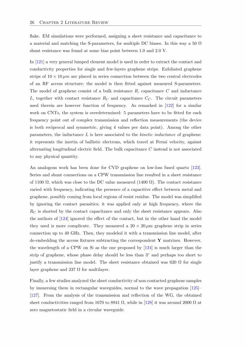
26 Chapter 2 Literature Review
flake. EM simulations were performed, assigning a sheet resistance and capacitance to
a material and matching the S-parameters, for multiple DC biases. In this way a 50 Ω
shunt resistance was found at some bias point between 1.0 and 2.0 V.
In [121] a very general lumped element model is used in order to extract the contact and
conductivity properties for single and few-layers graphene strips. Exfoliated graphene
strips of 10 × 10µm are placed in series connection between the two central electrodes
of an RF access structure; the model is then fitted against measured S-parameters.
The model of graphene consist of a bulk resistance R, capacitance C and inductance
L, together with contact resistance RC and capacitance CC . The circuit parameters
used therein are however function of frequency. As remarked in [122] for a similar
work on CNTs, the system is overdetermined: 5 parameters have to be fitted for each
frequency point out of complex transmission and reflection measurements (the device
is both reciprocal and symmetric, giving 4 values per data point). Among the other
parameters, the inductance L is here associated to the kinetic inductance of graphene:
it represents the inertia of ballistic electrons, which travel at Fermi velocity, against
alternating longitudinal electric field. The bulk capacitance C instead is not associated
to any physical quantity.
An analogous work has been done for CVD graphene on low-loss fused quartz [123].
Series and shunt connections on a CPW transmission line resulted in a sheet resistance
of 1100 Ω, which was close to the DC value measured (1400 Ω). The contact resistance
varied with frequency, indicating the presence of a capacitive effect between metal and
graphene, possibly coming from local regions of resist residue. The model was simplified
by ignoring the contact parasitics; it was applied only at high frequency, where the
RC is shorted by the contact capacitance and only the sheet resistance appears. Also
the authors of [124] ignored the effect of the contact, but in the other hand the model
they used is more complicate. They measured a 20 × 20µm graphene strip in series
connection up to 40 GHz. Then, they modeled it with a transmission line model, after
de-embedding the access fixtures subtracting the correspondent Y matrixes. However,
the wavelength of a CPW on Si as the one proposed by [124] is much larger than the
strip of graphene, whose phase delay should be less than 3 and perhaps too short to
justify a transmission line model. The sheet resistance obtained was 620 Ω for single
layer graphene and 237 Ω for multilayer.
Finally, a few studies analyzed the sheet conductivity of non-contacted graphene samples
by immersing them in rectangular waveguides, normal to the wave propagation [125]–
[127]. From the analysis of the transmission and reflection of the WG, the obtained
sheet conductivities ranged from 1670 to 8941 Ω, while in [128] it was around 2000 Ω at
zero magnetostatic field in a circular waveguide.

2.5 Conclusions 27
2.5 Conclusions
The study of the metal/graphene contact and of the high-frequency propagation is
treated very differently among the various fields of study. They should be considered as
aspects of a same, larger, problem. However, the examinations of contact are carried out
only at zero frequency. A few empirical studies consider both aspects, but sometimes
with over-simplified models.
On the other hand, in FET modeling the contact parasitic is taken into account. Its
effects on high-frequency FOMs are deeply evaluated because of the severe impact on the
transconductance and output current. High frequency performances are the main target
of these experiments and models, stressing the importance of sub-micrometer scaling to
attain even higher performances. And yet, contact parasitics are generally represented
by a simple resistance, evaluated in DC and independent in frequency.
In conclusion, the need of a universal model connecting the finer investigation of the
physics involved in sub-micrometric FET devices and the high frequency propagation is
growing in importance. This work aims to bring near those two fields, putting the basis
for their integration in a single domain of study.
References
[1] K. S. Novoselov, a. K. Geim, S. V. Morozov, D. Jiang, Y. Zhang, S. V. Dubonos, I. V.
Grigorieva, and a. a. Firsov, “Electric field effect in atomically thin carbon films.”, Science
(New York, N.Y.), vol. 306, no. 5696, pp. 666–9, Oct. 2004. doi: 10.1126/science.
1102896.
[2] A. S. Mayorov, R. V. Gorbachev, S. V. Morozov, L. Britnell, R. Jalil, L. a. Ponomarenko,
P. Blake, K. S. Novoselov, K. Watanabe, T. Taniguchi, and a. K. Geim, “Micrometer-
scale ballistic transport in encapsulated graphene at room temperature.”, Nano letters,
vol. 11, no. 6, pp. 2396–9, Jun. 2011. doi: 10.1021/nl200758b.
[3] K. Bolotin, K. Sikes, Z. Jiang, M. Klima, G. Fudenberg, J. Hone, P. Kim, and H. Stormer,
“Ultrahigh electron mobility in suspended graphene”, Solid State Communications, vol.
146, no. 9-10, pp. 351–355, 2008.
[4] C. Berger, Z. Song, X. Li, X. Wu, N. Brown, C. Naud, D. Mayou, T. Li, J. Hass, A. N.
Marchenkov, E. H. Conrad, P. N. First, and W. a. de Heer, “Electronic confinement
and coherence in patterned epitaxial graphene.”, Science (New York, N.Y.), vol. 312, no.
5777, pp. 1191–6, May 2006. doi: 10.1126/science.1125925.

28 Chapter 2 Literature Review
[5] J. A. Robinson, M. Wetherington, J. L. Tedesco, P. M. Campbell, X. Weng, J. Stitt, M. a.
Fanton, E. Frantz, D. Snyder, B. L. VanMil, G. G. Jernigan, R. L. Myers-Ward, C. R.
Eddy, and D. K. Gaskill, “Correlating Raman spectral signatures with carrier mobility in
epitaxial graphene: a guide to achieving high mobility on the wafer scale.”, Nano letters,
vol. 9, no. 8, pp. 2873–6, Aug. 2009. doi: 10.1021/nl901073g.
[6] Z. Guo, R. Dong, P. S. Chakraborty, N. Lourenco, J. Palmer, Y. Hu, M. Ruan, J. Hankin-
son, J. Kunc, J. D. Cressler, C. Berger, and W. a. de Heer, “Record maximum oscillation
frequency in C-face epitaxial graphene transistors.”, Nano letters, vol. 13, no. 3, pp. 942–
7, Mar. 2013. doi: 10.1021/nl303587r.
[7] S. Y. Zhou, G.-H. Gweon, A. V. Fedorov, P. N. First, W. A. de Heer, D.-H. Lee, F.
Guinea, A. H. Castro Neto, and A. Lanzara, “Substrate-induced bandgap opening in
epitaxial graphene.”, Nature materials, vol. 6, no. 10, pp. 770–5, Oct. 2007. doi: 10.
1038/nmat2003. arXiv: 0709.1706.
[8] N. Ferralis, R. Maboudian, and C. Carraro, “Evidence of structural strain in epitaxial
graphene layers on 6H-SiC(0001)”, Physical Review Letters, vol. 101, p. 156 801, 2008.
[9] F. Schwierz, “Graphene Transistors: Status, Prospects, and Problems”, Proceedings of
the IEEE, vol. 101, no. 7, pp. 1567–1584, Jul. 2013. doi: 10.1109/JPROC.2013.2257633.
[10] W. A. de Heer, C. Berger, M. Ruan, M. Sprinkle, X. Li, Y. Hu, B. Zhang, J. Hankinson,
and E. Conrad, “Large area and structured epitaxial graphene produced by confinement
controlled sublimation of silicon carbide.”, Proceedings of the National Academy of Sci-
ences of the United States of America, vol. 108, no. 41, pp. 16 900–5, Oct. 2011. doi:
10.1073/pnas.1105113108.
[11] Y. Lin, D. Farmer, and K. Jenkins, “Enhanced Performance in Epitaxial Graphene FETs
With Optimized Channel Morphology”, Electron Device, vol. 32, no. 10, pp. 1343–1345,
2011.
[12] X. Li, W. Cai, J. An, S. Kim, J. Nah, D. Yang, R. Piner, A. Velamakanni, I. Jung, E.
Tutuc, S. K. Banerjee, L. Colombo, and R. S. Ruoff, “Large-area synthesis of high-quality
and uniform graphene films on copper foils.”, Science (New York, N.Y.), vol. 324, no.
5932, pp. 1312–4, Jun. 2009. doi: 10.1126/science.1171245.
[13] P. J. Ko, H. Takahashi, S. Koide, H. Sakai, T. V. Thu, H. Okada, and A. Sandhu, “Simple
method to transfer graphene from metallic catalytic substrates to flexible surfaces without
chemical etching”, Journal of Physics: Conference Series, vol. 433, p. 012 002, Apr. 2013.
doi: 10.1088/1742-6596/433/1/012002.
[14] S. Bae, H. Kim, Y. Lee, X. Xu, J.-S. Park, Y. Zheng, J. Balakrishnan, T. Lei, H. R. Kim,
Y. I. Song, Y.-J. Kim, K. S. Kim, B. Ozyilmaz, J.-H. Ahn, B. H. Hong, and S. Iijima,
“Roll-to-roll production of 30-inch graphene films for transparent electrodes.”, Nature
nanotechnology, vol. 5, no. 8, pp. 574–8, Aug. 2010. doi: 10.1038/nnano.2010.132.

REFERENCES 29
[15] T. Kobayashi, M. Bando, N. Kimura, K. Shimizu, K. Kadono, N. Umezu, K. Miyahara,
S. Hayazaki, S. Nagai, Y. Mizuguchi, Y. Murakami, and D. Hobara, “Production of a 100-
m-long high-quality graphene transparent conductive film by roll-to-roll chemical vapor
deposition and transfer process”, Applied Physics Letters, vol. 102, no. 2, p. 023 112, 2013.
doi: 10.1063/1.4776707.
[16] A. Pirkle, J. Chan, A. Venugopal, D. Hinojos, C. W. Magnuson, S. McDonnell, L.
Colombo, E. M. Vogel, R. S. Ruoff, and R. M. Wallace, “The effect of chemical residues on
the physical and electrical properties of chemical vapor deposited graphene transferred to
SiO2”, Applied Physics Letters, vol. 99, no. 12, p. 122 108, 2011. doi: 10.1063/1.3643444.
[17] Y. Hernandez, V. Nicolosi, M. Lotya, F. M. Blighe, Z. Sun, S. De, I. T. McGovern, B.
Holland, M. Byrne, Y. K. Gun’Ko, J. J. Boland, P. Niraj, G. Duesberg, S. Krishnamurthy,
R. Goodhue, J. Hutchison, V. Scardaci, A. C. Ferrari, and J. N. Coleman, “High-yield
production of graphene by liquid-phase exfoliation of graphite.”, Nature nanotechnology,
vol. 3, no. 9, pp. 563–8, Sep. 2008. doi: 10.1038/nnano.2008.215.
[18] A. a. Green and M. C. Hersam, “Solution phase production of graphene with controlled
thickness via density differentiation.”, Nano letters, vol. 9, no. 12, pp. 4031–6, Dec. 2009.
doi: 10.1021/nl902200b.
[19] G. Eda, G. Fanchini, and M. Chhowalla, “Large-area ultrathin films of reduced graphene
oxide as a transparent and flexible electronic material.”, Nature nanotechnology, vol. 3,
no. 5, pp. 270–4, May 2008. doi: 10.1038/nnano.2008.83.
[20] M. F. El-Kady, V. Strong, S. Dubin, and R. B. Kaner, “Laser scribing of high-performance
and flexible graphene-based electrochemical capacitors.”, Science (New York, N.Y.), vol.
335, no. 6074, pp. 1326–30, Mar. 2012. doi: 10.1126/science.1216744.
[21] K. S. Novoselov, V. I. Fal’ko, L. Colombo, P. R. Gellert, M. G. Schwab, and K. Kim,
“A roadmap for graphene.”, Nature, vol. 490, no. 7419, pp. 192–200, Oct. 2012. doi:
10.1038/nature11458.
[22] P. Wallace, “The Band Theory of Graphite”, Physical Review, vol. 71, no. 9, pp. 622–634,
May 1947. doi: 10.1103/PhysRev.71.622.
[23] R. E. Peierls, “Quelques proprietes typiques des corpses solides”, Ann. I. H. Poincare,
vol. 5, pp. 177–222, 1935.
[24] J. McClure, “Band Structure of Graphite and de Haas-van Alphen Effect”, Physical
Review, vol. 108, no. 3, pp. 612–618, Nov. 1957. doi: 10.1103/PhysRev.108.612.
[25] J. Slonczewski and P. Weiss, “Band Structure of Graphite”, Physical Review, vol. 109,
no. 2, pp. 272–279, Jan. 1958. doi: 10.1103/PhysRev.109.272.
[26] S. Reich, J. Maultzsch, C. Thomsen, and P. Ordejon, “Tight-binding description of
graphene”, Physical Review B, vol. 66, no. 3, p. 035 412, Jul. 2002. doi: 10 . 1103 /
PhysRevB.66.035412.
[27] A. Castro Neto, F. Guinea, N. Peres, K. Novoselov, and A. Geim, “The electronic prop-
erties of graphene”, Reviews of Modern Physics, vol. 81, no. 1, pp. 109–162, Jan. 2009.
doi: 10.1103/RevModPhys.81.109.

30 Chapter 2 Literature Review
[28] V. Ariel and A. Natan, “Electron Effective Mass in Graphene”, arXiv pre-print, p. 1206.6100,
Jun. 2012. arXiv: 1206.6100.
[29] T. Fang, A. Konar, H. Xing, and D. Jena, “Carrier statistics and quantum capacitance
of graphene sheets and ribbons”, Applied Physics Letters, vol. 91, no. 9, p. 092 109, 2007.
doi: 10.1063/1.2776887. arXiv: 0707.2242v1.
[30] A. Fasolino, J. H. Los, and M. I. Katsnelson, “Intrinsic ripples in graphene.”, Nature
materials, vol. 6, no. 11, pp. 858–61, Nov. 2007. doi: 10.1038/nmat2011.
[31] D. Reddy, L. F. Register, G. D. Carpenter, and S. K. Banerjee, “Graphene field-effect
transistors”, Journal of Physics D: Applied Physics, vol. 45, no. 1, p. 019 501, Jan. 2012.
doi: 10.1088/0022-3727/45/1/019501.
[32] K. D. Holland, N. Paydavosi, N. Neophytou, D. Kienle, and M. Vaidyanathan, “RF Per-
formance Limits and Operating Physics Arising From the Lack of a Bandgap in Graphene
Transistors”, IEEE Transactions on Nanotechnology, vol. 12, no. 4, pp. 566–577, Jul. 2013.
doi: 10.1109/TNANO.2013.2260351.
[33] K. Wakabayashi, M. Fujita, H. Ajiki, and M. Sigrist, “Electronic and magnetic properties
of nanographite ribbons”, Physical Review B, vol. 59, no. 12, pp. 8271–8282, Mar. 1999.
doi: 10.1103/PhysRevB.59.8271.
[34] M. Han, B. Ozyilmaz, Y. Zhang, and P. Kim, “Energy Band-Gap Engineering of Graphene
Nanoribbons”, Physical Review Letters, vol. 98, no. 20, p. 206 805, May 2007. doi: 10.
1103/PhysRevLett.98.206805.
[35] P. Gallagher, K. Todd, and D. Goldhaber-Gordon, “Disorder-induced gap behavior in
graphene nanoribbons”, Physical Review B, vol. 81, no. 11, p. 115 409, Mar. 2010. doi:
10.1103/PhysRevB.81.115409.
[36] M. Y. Han, J. C. Brant, and P. Kim, “Electron Transport in Disordered Graphene
Nanoribbons”, Physical Review Letters, vol. 104, no. 5, p. 056 801, Feb. 2010. doi: 10.
1103/PhysRevLett.104.056801.
[37] A. Pieper, G. Schubert, G. Wellein, and H. Fehske, “Effects of disorder and contacts on
transport through graphene nanoribbons”, vol. cond-mat.m, Aug. 2013. arXiv: 1308.
6079.
[38] Y. Yang and R. Murali, “Impact of Size Effect on Graphene Nanoribbon Transport”,
IEEE Electron Device Letters, vol. 31, no. 3, pp. 237–239, Mar. 2010. doi: 10.1109/LED.
2009.2039915.
[39] O. Habibpour, J. Vukusic, and J. Stake, “A 30-GHz Integrated Subharmonic Mixer Based
on a Multichannel Graphene FET”, IEEE Transactions on Microwave Theory and Tech-
niques, vol. 61, no. 2, pp. 841–847, Feb. 2013. doi: 10.1109/TMTT.2012.2236434.
[40] N. Meng, J. F. Fernandez, D. Vignaud, G. Dambrine, and H. Happy, “Fabrication and
Characterization of an Epitaxial Graphene Nanoribbon-Based Field-Effect Transistor”,
IEEE Transactions on Electron Devices, vol. 58, no. 6, pp. 1594–1596, Jun. 2011. doi:
10.1109/TED.2011.2119486.

REFERENCES 31
[41] K. Yan, H. Peng, Y. Zhou, H. Li, and Z. Liu, “Formation of bilayer bernal graphene: layer-
by-layer epitaxy via chemical vapor deposition.”, Nano letters, vol. 11, no. 3, pp. 1106–10,
Mar. 2011. doi: 10.1021/nl104000b.
[42] L. Liu, H. Zhou, R. Cheng, W. J. Yu, Y. Liu, Y. Chen, J. Shaw, X. Zhong, Y. Huang,
and X. Duan, “High-yield chemical vapor deposition growth of high-quality large-area
AB-stacked bilayer graphene.”, ACS nano, vol. 6, no. 9, pp. 8241–9, Sep. 2012. doi:
10.1021/nn302918x.
[43] F. Xia, D. B. Farmer, Y.-M. Lin, and P. Avouris, “Graphene field-effect transistors with
high on/off current ratio and large transport band gap at room temperature.”, Nano
letters, vol. 10, no. 2, pp. 715–8, Feb. 2010. doi: 10.1021/nl9039636.
[44] L. Britnell, R. V. Gorbachev, R. Jalil, B. D. Belle, F. Schedin, a. Mishchenko, T. Georgiou,
M. I. Katsnelson, L. Eaves, S. V. Morozov, N. M. R. Peres, J. Leist, a. K. Geim, K. S.
Novoselov, and L. a. Ponomarenko, “Field-effect tunneling transistor based on vertical
graphene heterostructures.”, Science (New York, N.Y.), vol. 335, no. 6071, pp. 947–50,
Feb. 2012. doi: 10.1126/science.1218461.
[45] S. Vaziri, G. Lupina, C. Henkel, A. D. Smith, M. Ostling, J. Dabrowski, G. Lippert, W.
Mehr, and M. C. Lemme, “A graphene-based hot electron transistor.”, Nano letters, vol.
13, no. 4, pp. 1435–9, Apr. 2013. doi: 10.1021/nl304305x.
[46] C. Zeng, E. B. Song, M. Wang, S. Lee, C. M. Torres, J. Tang, B. H. Weiller, and K. L.
Wang, “Vertical graphene-base hot-electron transistor.”, Nano letters, vol. 13, no. 6,
pp. 2370–5, Jun. 2013. doi: 10.1021/nl304541s.
[47] W. Mehr, J. Dabrowski, J. C. Scheytt, G. Lippert, Y.-h. Xie, M. C. Lemme, M. Ostling,
and G. Lupina, “Vertical Graphene Base Transistor”, IEEE Electron Device Letters, vol.
33, no. 5, pp. 691–693, May 2012. doi: 10.1109/LED.2012.2189193.
[48] H. Hsu and L. Reichl, “Modeling graphene layers and single-walled carbon nanotubes
with regularized δ-function potentials”, Physical Review B, vol. 72, no. 15, p. 155 413,
Oct. 2005. doi: 10.1103/PhysRevB.72.155413.
[49] A. K. Geim and K. S. Novoselov, “The rise of graphene.”, Nature materials, vol. 6, no.
3, pp. 183–91, Mar. 2007. doi: 10.1038/nmat1849.
[50] Y.-W. Son, M. L. Cohen, and S. G. Louie, “Energy Gaps in Graphene Nanoribbons”,
Physical Review Letters, vol. 97, no. 21, p. 216 803, Nov. 2006. doi: 10.1103/PhysRevLett.
97.216803.
[51] V. Barone, O. Hod, and G. E. Scuseria, “Electronic structure and stability of semicon-
ducting graphene nanoribbons.”, Nano letters, vol. 6, no. 12, pp. 2748–54, Dec. 2006. doi:
10.1021/nl0617033.
[52] G. Fiori and G. Iannaccone, “Simulation of Graphene Nanoribbon Field-Effect Tran-
sistors”, IEEE Electron Device Letters, vol. 28, no. 8, pp. 760–762, Aug. 2007. doi:
10.1109/LED.2007.901680.
[53] Y. Hancock, A. Uppstu, K. Saloriutta, A. Harju, and M. J. Puska, “Generalized tight-
binding transport model for graphene nanoribbon-based systems”, Physical Review B,
vol. 81, no. 24, pp. 3–8, Jun. 2010. doi: 10.1103/PhysRevB.81.245402.

32 Chapter 2 Literature Review
[54] Y. Ouyang, Y. Yoon, J. K. Fodor, and J. Guo, “Comparison of performance limits for
carbon nanoribbon and carbon nanotube transistors”, Applied Physics Letters, vol. 89,
no. 20, p. 203 107, 2006. doi: 10.1063/1.2387876.
[55] G. Liang, N. Neophytou, D. E. Nikonov, and M. S. Lundstrom, “Performance Projec-
tions for Ballistic Graphene Nanoribbon Field-Effect Transistors”, IEEE Transactions on
Electron Devices, vol. 54, no. 4, pp. 677–682, Apr. 2007. doi: 10.1109/TED.2007.891872.
[56] P. Zhao, M. Choudhury, K. Mohanram, and J. Guo, “Computational Model of Edge
Effects in Graphene Nanoribbon Transistors”, 2008. doi: 10.1007/s12274-008-8039-y.
[57] V. Ryzhii, M. Ryzhii, A. Satou, and T. Otsuji, “Current-voltage characteristics of a
graphene-nanoribbon field-effect transistor”, Journal of Applied Physics, vol. 103, no. 9,
p. 094 510, 2008. doi: 10.1063/1.2917284.
[58] W. Liu, X. Jin, X. Xi, J. Chen, M.-C. Jeng, Z. Liu, Y. Cheng, K. Chen, M. Chan, K. Hui,
J. Huang, R. Tu, P. K. Ko, and C. Hu, BSIM3v3.3 MOSFET Model, Berkeley, 2005.
[59] A. Khakifirooz, O. M. Nayfeh, and D. Antoniadis, “A Simple Semiempirical Short-
Channel MOSFET Current–Voltage Model Continuous Across All Regions of Operation
and Employing Only Physical Parameters”, IEEE Transactions on Electron Devices, vol.
56, no. 8, pp. 1674–1680, Aug. 2009. doi: 10.1109/TED.2009.2024022.
[60] I. Meric, M. Y. Han, A. F. Young, B. Ozyilmaz, P. Kim, and K. L. Shepard, “Current sat-
uration in zero-bandgap, top-gated graphene field-effect transistors.”, Nature nanotech-
nology, vol. 3, no. 11, pp. 654–9, Nov. 2008. doi: 10.1038/nnano.2008.268.
[61] H. Wang, A. Hsu, J. Kong, D. A. Antoniadis, and T. Palacios, “Compact Virtual-Source
Current–Voltage Model for Top- and Back-Gated Graphene Field-Effect Transistors”,
IEEE Transactions on Electron Devices, vol. 58, no. 5, pp. 1523–1533, May 2011. doi:
10.1109/TED.2011.2118759.
[62] E. Mucciolo, A. Castro Neto, and C. Lewenkopf, “Conductance quantization and trans-
port gaps in disordered graphene nanoribbons”, Physical Review B, vol. 79, no. 7, p. 075 407,
Feb. 2009. doi: 10.1103/PhysRevB.79.075407.
[63] K. Ganapathi, Y. Yoon, M. Lundstrom, and S. Salahuddin, “Ballistic ¡formula formu-
latype=”inline”¿¡tex Notation=”TeX”¿$I$¡/tex¿¡/formula¿– ¡formula formulatype=”inline”¿¡tex
Notation=”TeX”¿$V$¡/tex¿¡/formula¿ Characteristics of Short-Channel Graphene Field-
Effect Transistors: Analysis and Optimization for Analog”, IEEE Transactions on Elec-
tron Devices, vol. 60, no. 3, pp. 958–964, Mar. 2013. doi: 10.1109/TED.2013.2238236.
[64] D. Mencarelli, T. Rozzi, and L. Pierantoni, “Scattering matrix approach to multichan-
nel transport in many lead graphene nanoribbons.”, Nanotechnology, vol. 21, no. 15,
p. 155 701, Apr. 2010. doi: 10.1088/0957-4484/21/15/155701.
[65] D. Mencarelli, L. Pierantoni, and T. Rozzi, “Graphene modeling by TLM approach”, in
2012 IEEE/MTT-S International Microwave Symposium Digest, IEEE, Jun. 2012, pp. 1–
3. doi: 10.1109/MWSYM.2012.6259782.
[66] X. Yang, G. Fiori, G. Iannaccone, and K. Mohanram, “Semi-analytical Model for Schottky-
barrier Carbon Nanotube and Graphene Nanoribbon Transistors”, in Proceedings of the
20th symposium on Great lakes symposium on VLSI, 2010, pp. 233–238.

REFERENCES 33
[67] A. Rahman, S. Datta, and M. Lundstrom, “Theory of ballistic nanotransistors”, IEEE
Transactions on Electron Devices, vol. 50, no. 9, pp. 1853–1864, Sep. 2003. doi: 10.1109/
TED.2003.815366.
[68] R. Landauer, “Spatial variation of currents and fields due to localized scatterers in metallic
conduction”, IBM Journal of Research and Development, vol. 32, no. 3, pp. 306–316, May
1988. doi: 10.1147/rd.323.0306.
[69] K. Natori, “Ballistic metal-oxide-semiconductor field effect transistor”, Journal of Applied
Physics, vol. 76, no. 8, p. 4879, 1994. doi: 10.1063/1.357263.
[70] D. Jimenez, “A current-voltage model for Schottky-barrier graphene-based transistors.”,
Nanotechnology, vol. 19, no. 34, p. 345 204, Aug. 2008. doi: 10.1088/0957-4484/19/34/
345204.
[71] G. S. Kliros, “Gate capacitance modeling and width-dependent performance of graphene
nanoribbon transistors”, Microelectronic Engineering, Apr. 2013. doi: 10.1016/j.mee.
2013.04.011.
[72] V. Ryzhii, M. Ryzhii, A. Satou, T. Otsuji, and V. Mitin, “Analytical device model for
graphene bilayer field-effect transistors using weak nonlocality approximation”, Journal
of Applied Physics, vol. 109, no. 6, p. 064 508, 2011. doi: 10.1063/1.3560921.
[73] F. Schwierz, “Graphene transistors”, Nature Nanotechnology, vol. 5, no. 7, pp. 487–496,
May 2010. doi: 10.1038/nnano.2010.89.
[74] S. Thiele and F. Schwierz, “Modeling of the steady state characteristics of large-area
graphene field-effect transistors”, Journal of Applied Physics, vol. 110, no. 3, p. 034 506,
2011. doi: 10.1063/1.3606583.
[75] J. G. Champlain, “A first principles theoretical examination of graphene-based field effect
transistors”, Journal of Applied Physics, vol. 109, no. 8, p. 084 515, 2011. doi: 10.1063/
1.3573517.
[76] V. Ryzhii, M. Ryzhii, A. Satou, T. Otsuji, and N. Kirova, “Device model for graphene
bilayer field-effect transistor”, Journal of Applied Physics, vol. 105, no. 10, p. 104 510,
2009. doi: 10.1063/1.3131686.
[77] G. I. Zebrev, A. A. Tselykovskiy, and V. O. Turin, “Physics-based compact modeling of
double-gate graphene field-effect transistor operation”, in 2012 28th International Con-
ference on Microelectronics Proceedings, IEEE, May 2012, pp. 237–240. doi: 10.1109/
MIEL.2012.6222843. arXiv: 1110.6319.
[78] I. Umoh and T. Kazmierski, “VHDL-AMS model of a dual gate graphene FET”, in
Specification and Design Languages (FDL), 2011 Forum on, vol. 2, Oldenburg: IEEE,
2011, pp. 1–5.
[79] I. J. Umoh, T. J. Kazmierski, and B. M. Al-Hashimi, “A Dual-Gate Graphene FET Model
for Circuit Simulation—SPICE Implementation”, IEEE Transactions on Nanotechnology,
vol. 12, no. 3, pp. 427–435, May 2013. doi: 10.1109/TNANO.2013.2253490.
[80] K. N. Parrish, M. E. Ramon, S. K. Banerjee, and D. Akinwande, “A Compact Model for
Graphene FETs for Linear and Non-linear Circuits”, in SISPAD 2012, 2012, pp. 75–78.

34 Chapter 2 Literature Review
[81] W. Liu, MOSFET Models for SPICE Simulation: Including BSIM3v3 and BSIM4. Wiley-
IEEE Press, 2011, ch. 1.3, p. 600.
[82] K. N. Parrish and D. Akinwande, “Impact of contact resistance on the transconductance
and linearity of graphene transistors”, Applied Physics Letters, vol. 98, no. 18, p. 183 505,
2011. doi: 10.1063/1.3582613.
[83] “International Technology Roadmap for Semiconductors - Emerging Research Materials”,
International Roadmap Committee, Tech. Rep., 2011.
[84] I. R. Committee, “International Technology Roadmap for Semiconductors - Intercon-
nects”, Semiconductor Industry Association, Tech. Rep., 2011.
[85] F. Xia, V. Perebeinos, Y.-m. Lin, Y. Wu, and P. Avouris, “The origins and limits of
metal-graphene junction resistance.”, Nature nanotechnology, vol. 6, no. 3, pp. 179–84,
Mar. 2011. doi: 10.1038/nnano.2011.6.
[86] K. L. Grosse, M.-H. Bae, F. Lian, E. Pop, and W. P. King, “Nanoscale Joule heating,
Peltier cooling and current crowding at graphene-metal contacts.”, Nature nanotechnol-
ogy, vol. 6, no. 5, pp. 287–90, May 2011. doi: 10.1038/nnano.2011.39.
[87] K. Nagashio, T. Nishimura, K. Kita, and A. Toriumi, “Contact resistivity and current
flow path at metal/graphene contact”, Applied Physics Letters, vol. 97, no. 14, p. 143 514,
2010. doi: 10.1063/1.3491804.
[88] A. D. Franklin, S.-j. Han, A. A. Bol, and V. Perebeinos, “Double Contacts for Improved
Performance of Graphene Transistors”, IEEE Electron Device Letters, pp. 4–6, 2011. doi:
10.1109/LED.2011.2173154.
[89] C. Malec and D. Davidovic, “Electronic properties of Au-graphene contacts”, Physical
Review B, vol. 84, no. 3, pp. 4–7, Jul. 2011. doi: 10.1103/PhysRevB.84.033407.
[90] J. S. Moon, M. Antcliffe, H. C. Seo, D. Curtis, S. Lin, A. Schmitz, I. Milosavljevic, A. A.
Kiselev, R. S. Ross, D. K. Gaskill, P. M. Campbell, R. C. Fitch, K.-M. Lee, and P. Asbeck,
“Ultra-low resistance ohmic contacts in graphene field effect transistors”, Applied Physics
Letters, vol. 100, no. 20, p. 203 512, 2012. doi: 10.1063/1.4719579.
[91] J. T. Smith, A. D. Franklin, D. B. Farmer, and C. D. Dimitrakopoulos, “Reducing Contact
Resistance in Graphene Devices through Contact Area Patterning.”, ACS nano, no. Xx,
Mar. 2013. doi: 10.1021/nn400671z.
[92] C. Malec, B. Elkus, and D. Davidovic, “Vacuum-annealed Cu contacts for graphene elec-
tronics”, Solid State Communications, vol. 151, no. 23, pp. 1791–1793, Dec. 2011. doi:
10.1016/j.ssc.2011.08.025.
[93] B. Huard, N. Stander, J. Sulpizio, and D. Goldhaber-Gordon, “Evidence of the role of
contacts on the observed electron-hole asymmetry in graphene”, Physical Review B, vol.
78, no. 12, Sep. 2008. doi: 10.1103/PhysRevB.78.121402.
[94] D. B. Farmer, R. Golizadeh-Mojarad, V. Perebeinos, Y.-M. Lin, G. S. Tulevski, J. C.
Tsang, and P. Avouris, “Chemical doping and electron-hole conduction asymmetry in
graphene devices.”, Nano letters, vol. 9, no. 1, pp. 388–92, Jan. 2009. doi: 10.1021/
nl803214a.

REFERENCES 35
[95] T. Mueller, F. Xia, M. Freitag, J. Tsang, and P. Avouris, “Role of contacts in graphene
transistors: A scanning photocurrent study”, Physical Review B, vol. 79, no. 24, p. 245 430,
2009. doi: 10.1103/PhysRevB.79.245430.
[96] B. Huard, J. Sulpizio, N. Stander, K. Todd, B. Yang, and D. Goldhaber-Gordon, “Trans-
port Measurements Across a Tunable Potential Barrier in Graphene”, Physical Review
Letters, vol. 98, no. 23, pp. 8–11, Jun. 2007. doi: 10.1103/PhysRevLett.98.236803.
[97] G. Giovannetti, P. Khomyakov, G. Brocks, V. Karpan, J. Van Den Brink, and P. Kelly,
“Doping graphene with metal contacts”, Physical review letters, vol. 101, no. 2, p. 26 803,
2008.
[98] P. Khomyakov, G. Giovannetti, P. Rusu, G. Brocks, J. van Den Brink, and P. Kelly,
“First-principles study of the interaction and charge transfer between graphene and met-
als”, Physical Review B, vol. 79, no. 19, p. 195 425, May 2009. doi: 10.1103/PhysRevB.
79.195425.
[99] G. Kotliar, S. Savrasov, K. Haule, V. Oudovenko, O. Parcollet, and C. Marianetti,
“Electronic structure calculations with dynamical mean-field theory”, Reviews of Modern
Physics, vol. 78, no. 3, pp. 865–951, Aug. 2006. doi: 10.1103/RevModPhys.78.865.
[100] C. Gong, G. Lee, B. Shan, E. M. Vogel, R. M. Wallace, and K. Cho, “First-principles study
of metal–graphene interfaces”, Journal of Applied Physics, vol. 108, no. 12, p. 123 711,
2010. doi: 10.1063/1.3524232.
[101] J. S lawinska, P. Dabrowski, and I. Zasada, “Doping of graphene by a Au(111) substrate:
Calculation strategy within the local density approximation and a semiempirical van
der Waals approach”, Physical Review B, vol. 83, no. 24, p. 245 429, Jun. 2011. doi:
10.1103/PhysRevB.83.245429.
[102] J. Granatier, P. Lazar, M. Otyepka, and P. Hobza, “The Nature of the Binding of Au, Ag,
and Pd to Benzene, Coronene, and Graphene: From Benchmark CCSD(T) Calculations
to Plane-Wave DFT Calculations.”, Journal of chemical theory and computation, vol. 7,
no. 11, pp. 3743–3755, Nov. 2011. doi: 10.1021/ct200625h.
[103] K. Nagashio and A. Toriumi, “Density-of-States Limited Contact Resistance in Graphene
Field-Effect Transistors”, Japanese Journal of Applied Physics, vol. 50, no. 7, p. 070 108,
Jul. 2011. doi: 10.1143/JJAP.50.070108.
[104] S. Barraza-Lopez, M. Vanevic, M. Kindermann, and M. Y. Chou, “Effects of Metallic
Contacts on Electron Transport through Graphene”, Physical Review Letters, vol. 104,
no. 7, p. 076 807, Feb. 2010. doi: 10.1103/PhysRevLett.104.076807.
[105] P. Khomyakov, A. Starikov, G. Brocks, and P. Kelly, “Nonlinear screening of charges
induced in graphene by metal contacts”, Physical Review B, vol. 82, no. 11, p. 115 437,
Sep. 2010. doi: 10.1103/PhysRevB.82.115437.
[106] R. Nouchi and K. Tanigaki, “Empirical Modeling of Metal-Contact Effects on Graphene
Field-Effect Transistors”, Japanese Journal of Applied Physics, vol. 50, no. 7, p. 070 109,
Jul. 2011. doi: 10.1143/JJAP.50.070109.

36 Chapter 2 Literature Review
[107] Z. Chen and J. Appenzeller, “Gate modulation of graphene contacts – on the scaling of
graphene FETs”, in VLSI Technology, 2009 Symposium on, Honolulu, HI, 2009, pp. 128–
129.
[108] D. Berdebes, T. Low, Y. Sui, J. Appenzeller, and M. S. Lundstrom, “Substrate Gating of
Contact Resistance in Graphene Transistors”, IEEE Transactions on Electron Devices,
vol. 58, no. 11, pp. 3925–3932, Nov. 2011. doi: 10.1109/TED.2011.2163800.
[109] A. D. Franklin, S.-j. Han, A. A. Bol, and W. Haensch, “Effects of Nanoscale Contacts to
Graphene”, IEEE Electron Device Letters, vol. 32, no. 8, pp. 1035–1037, Aug. 2011. doi:
10.1109/LED.2011.2158058.
[110] H. Berger, “Models for contacts to planar devices”, Solid-State Electronics, vol. 15, no.
2, pp. 145–158, Feb. 1972. doi: 10.1016/0038-1101(72)90048-2.
[111] D. Schroder, Semiconductor material and device characterization. John Wiley & Sons,
2006.
[112] C. Lan, P. Srisungsitthisunti, P. B. Amama, T. S. Fisher, X. Xu, and R. G. Reifenberger,
“Measurement of metal/carbon nanotube contact resistance by adjusting contact length
using laser ablation.”, Nanotechnology, vol. 19, no. 12, p. 125 703, Mar. 2008. doi: 10.
1088/0957-4484/19/12/125703.
[113] C. Lan, D. N. Zakharov, and R. G. Reifenberger, “Determining the optimal contact length
for a metal/multiwalled carbon nanotube interconnect”, Applied Physics Letters, vol. 92,
no. 21, p. 213 112, 2008. doi: 10.1063/1.2931081.
[114] K. Nagashio, T. Moriyama, R. Ifuku, T. Yamashita, T. Nishimura, and A. Toriumi, “Is
Graphene Contacting with Metal Still Graphene ?”, in International Electron Devices
Meeting 2011, vol. 5, 2011, pp. 27–30.
[115] W. Shockley, A. Goetzberger, and R. Scarlett, “Research and Investigation of Inverse
Epitaxial UHF Power Transistors”, Air Force Avionics Lab., Wright-Patterson Air Force
Base, Tech. Rep., 1964, pages.
[116] D. Janes and K. Webb, “Error analysis leading to design criteria for transmission line
model characterization of ohmic contacts”, IEEE Transactions on Electron Devices, vol.
48, no. 4, pp. 758–766, Apr. 2001. doi: 10.1109/16.915721.
[117] L. Gutai, “Statistical modeling of transmission line model test structures. I. The effect of
inhomogeneities on the extracted contact parameters”, IEEE Transactions on Electron
Devices, vol. 37, no. 11, pp. 2350–2360, 1990. doi: 10.1109/16.62287.
[118] G. S. Marlow and M. B. Das, “The effects of contact size and non-zero metal resistance
on the determination of specific contact resistance”, Solid-State Electronics, vol. 25, no.
2, pp. 91–94, Feb. 1982. doi: 10.1016/0038-1101(82)90036-3.
[119] M. Dragoman, D. Dragoman, G. Deligiorgis, G. Konstantinidis, D. Neculoiu, A. Cismaru,
and R. Plana, “Current oscillations in a wide graphene sheet”, Journal of Applied Physics,
vol. 106, no. 4, p. 044 312, 2009. doi: 10.1063/1.3208061.
[120] G. Deligeorgis, M. Dragoman, D. Neculoiu, D. Dragoman, G. Konstantinidis, A. Cismaru,
and R. Plana, “Microwave propagation in graphene”, Applied Physics Letters, vol. 95, no.
7, p. 073 107, 2009. doi: 10.1063/1.3202413.

REFERENCES 37
[121] S. Moon, K. Jung, K. Park, H. Jin Kim, C.-W. Lee, C.-W. Baik, and J. M. Kim, “Intrinsic
high-frequency characteristics of graphene layers”, New Journal of Physics, vol. 12, no.
11, p. 113 031, Nov. 2010. doi: 10.1088/1367-2630/12/11/113031.
[122] S. C. Jun, X. M. H. Huang, S. Moon, H. J. Kim, J. Hone, Y. W. Jin, and J. M. Kim,
“Passive electrical properties of multi-walled carbon nanotubes up to 0.1 THz”, New
Journal of Physics, vol. 9, no. 8, pp. 265–265, Aug. 2007. doi: 10.1088/1367-2630/9/
8/265.
[123] H. S. Skulason, H. V. Nguyen, a. Guermoune, V. Sridharan, M. Siaj, C. Caloz, and T.
Szkopek, “110 GHz measurement of large-area graphene integrated in low-loss microwave
structures”, Applied Physics Letters, vol. 99, no. 15, p. 153 504, 2011. doi: 10.1063/1.
3650710.
[124] H.-J. Lee, E. Kim, J.-G. Yook, and J. Jung, “Intrinsic characteristics of transmission
line of graphenes at microwave frequencies”, Applied Physics Letters, vol. 100, no. 22,
p. 223 102, 2012. doi: 10.1063/1.4722585.
[125] N. Rouhi, D. Jain, S. Capdevila, L. Jofre, E. Brown, and P. J. Burke, “Broadband con-
ductivity of graphene from DC to THz”, in 2011 11th IEEE International Conference on
Nanotechnology, IEEE, Aug. 2011, pp. 1205–1207. doi: 10.1109/NANO.2011.6144485.
[126] J. S. Gomez-Dıaz, J. Perruisseau-Carrier, P. Sharma, and A. Ionescu, “Non-contact char-
acterization of graphene surface impedance at micro and millimeter waves”, Journal of
Applied Physics, vol. 111, no. 11, p. 114 908, 2012. doi: 10.1063/1.4728183.
[127] P. Sharma, J. Gomez-Diaz, A. Ionescu, and J. Perruisseau-Carrier, “Determination of
minimum conductivity of graphene from contactless microwaves measurements”, in Nan-
otechnology (IEEE-NANO), 2012 12th IEEE Conference on, 2012, pp. 1–4. doi: 10.
1109/NANO.2012.6322060.
[128] D. L. Sounas, H. S. Skulason, H. V. Nguyen, A. Guermoune, M. Siaj, T. Szkopek, and
C. Caloz, “Faraday rotation in magnetically biased graphene at microwave frequencies”,
Applied Physics Letters, vol. 102, no. 19, p. 191 901, 2013. doi: 10.1063/1.4804437.


Chapter 3
Graphene DC model
In this chapter the work on the DC modeling of graphene active devices will be presented.
The described model is based on the Top of the Barrier approach, which is a physical
semi-analytical ballistic model [1].
3.1 Motivation
The great majority of models used today to simulate the I-V characteristics of graphene
devices are based on the Drift-Diffusion (DD) transport mechanism, upon which the
industrial-standard model for Si CMOS, the BSIM is founded as well. DD is based on
the assumption that in the channel of the transistor (or any other conductor) a certain
amount of scattering centers exists, and that the conductivity depends on how many
charge carriers there are and how frequently they collide with a scatterer; the carrier drift
velocity is a function of the longitudinal electric field (given by the drain bias) and of the
mobility and saturation velocity parameters. Voltage and current are related through
the Drude model. However, if scattering is absent, as in an ideal ballistic transistor, the
velocity of carriers assumes its maximum value: it is not anymore directly related to the
longitudinal electric field, but with the potential drop between source and drain instead.
DD models can include empirically the increase in saturation current that comes from
ballistic effects, for example through the Source End Limit Velocity model as done for Si
in BSIM4v4.7 [2], but their validity in regimes near to ideal ballistic transport becomes
questionable.
The peculiarity of graphene is to support a very limited amount of scattering even
at room temperature, especially when the interaction with the substrate is reduced
[3]. Moreover, at the same time that the quality of graphene samples improves, the
39

40 Chapter 3 Graphene DC model
channel lengths are scaled down too; this means that increasingly larger parts of the
electron conduction should rely on ballistic transport [4]. A ballistic model of graphene
nanotransistors becomes appropriate, but on the other hand their validity is generally
given only when ballistic transport is dominant [5].
Finally, many models fragment their operation in multiple segments or regimes, accord-
ing to the shape of the ID(VDS) curve (linear, quasi-saturation, second linear) or to
the type of charges within the channel (either electrons or holes, or both of them). In
this last context the word “ambipolar” is frequently used even if inappropriate [6]. The
fragmentation of the operation can lead to discontinuities in the gm or in its derivative.
3.2 Objectives of the study
This part of the work aims at finding a model that can correctly simulate both nanoscale
ballistic devices and microscale conventional Field Effect Transistors. This model should
rely on physical equations, with a minimal use of empirical parameters. Finally, its
operation should not be fragmented in different regimes.
3.3 Model: Top of the Barrier
In this section the discussion will be limited at the case of zero temperature. In the rest
of the chapter, room temperature will be taken into account. The Top of the Barrier is a
model that computes the carrier population of the channel of a transistor observing the
energy of the free carriers that it contains and the contacts. Considering a free carrier
at the edge of a contact, the barrier is the difference between the carrier’s energy, i.e. its
Fermi potential, and the closest-free-state energy in the channel. Carriers from source
and drain contacts are injected into the channel in a number dependent on the barrier’s
height towards each contact: in a condition of nonzero source-drain bias, each contact
causes a different amount of channel population, creating an unbalance between carriers
from the source and carriers from the drain. This non-equilibrium condition makes the
carriers move from source to drain, from the contact that fills the channel to the one
that depletes it, creating a current. If the free-state energy drops between the contact’s
energies, source and drain will inject respectively electrons and holes, and deplete the
opposite carrier type. Eventually the action of the gate electrode can be included by
shifting in energy the free states of the channel with a sign related to the gate bias
polarity, a magnitude non-linearly related to the gate voltage, the channel doping and
the injected carrier population. In the following sections each of those mechanisms will
be thoroughly detailed.

3.3 Model: Top of the Barrier 41
Figure 3.1: The cross-section of a graphene FET. Graphene is the black thick dottedline under contacts and gate oxide.
3.3.1 The Landauer Equation, carriers and contacts
In a top of the barrier framework either drift-diffusive (DD) or ballistic models can be
used. Examples of DD applications are in [7], [8], and for ballistic models in [1]. The
aim of this subsection is to describe the behavior of GNR-FET devices, in which small
dimensions and characteristics make the ballistic transport dominant. A cross-section
of the device is shown in Fig. 3.1. The Landauer equation will be used to quantify the
current of ballistic electrons and holes. By separating between the electron and hole
contributions, the drain current is given by [9]:
Id = In − Ip , (3.1)
where In and Ip correspond to electron and hole current respectively. A similar conven-
tion for all variables is followed throughout this chapter. The net current is given by
the difference of the injected electron and hole currents. In a simplified ballistic regime,
carriers are not subjected to recombination and are not exchanged between different
conducting states, thus they can be considered as independent fluxes. Moreover, no
energy relaxation into channel’s statistics is assumed as scattering is neglected [10]. As
opposed to DD, the Landauer equation allows for the computation of the current in a
device without scattering. Free states (or modes) are responsible for transport, and each
one of them is associated with a fixed conductivity q2/h, where q is the electron charge
and h is Planck’s constant. Injected electrons from each contact through the barrier are
described by the Fermi potential of their respective contact, and the injection unbalance
is the difference of the two Fermi functions fS and fD times the density of states Dn(E).
After integrating over energy, the electron current is given by:
In =vxq
2~
∫ +∞
−∞Dn(E) (fS − fD) dE . (3.2)

42 Chapter 3 Graphene DC model
where vx is the averaged carrier velocity, which is calculated from the energy dispersion
relation of the channel material. The dispersion relation is computed offline through
a full-quantum model, generally Tight Binding (TB) solved through Non-Equilibrium
Green’s Functions (NEGF) as in [11] for the case of a GNR. The hole current is com-
puted in a similar fashion. Differentiating the dispersion relation and averaging over all
available subbands and k-space yields the band velocity:
vx =1
2π
∫ +π/a
−π/a
1
N
N∑n=1
∣∣∣∣1~ dεn(k)
dk
∣∣∣∣dk , (3.3)
where k is the wavenumber, εn(k) is the energy of the n-th sub-band of the nanoribbon
and N is the number of unit cells. The averaging operation is a simplification with
respect to [1] where the carrier velocity is expressed as a function of energy (vx(E)), but
works around an intrinsic limit of the model. The geometry of the device is simplified
and, as it will be clearer from the electrostatics section, the channel is represented dimen-
sionlessly as a point. Carriers are injected at the top of the barrier, where their velocity
is minimum and kept constant all along the channel, neglecting carrier acceleration (in
a GNR, energy bands are parabolic as opposed to large area graphene where they show
the double-cone shape). Tests have been conducted and this results in underestimation
of the overall carrier velocity in the vx(E) model, especially for high biasing conditions.
Averaging its value over the entire k-space and all bands as in Eq. (3.3) can compen-
sate for this error [9]. Therefore, constant carrier velocity formulation was chosen being
both more accurate and simple compared to the energy-dependent expression. Finally,
this method allows a more coherent and unified framework including the simulation of
large-area graphene devices, which are in theory characterized by an energy independent
carrier velocity.
The density of states D(E) is analytically derived from the bandstructure [12]. To
account for impurities, the channel’s Fermi energy is shifted by the Dirac voltage, here
used as free parameter to describe the channel potential at zero bias. As the function
relating the gate voltage and the channel potential is strongly non-linear, it’s not possible
to retrieve the channel potential from, say, an ID−−VGS measure of the conductivity at
low drain bias; the lowest point in the V-shaped ID − −VGS indicates the gate voltage
at which the channel potential crosses the Charge Neutrality Point (CNP), but the
channel potential magnitude is generally smaller than the gate voltage. Its value must
be found iteratively by computing the minimum conductivity point in a low-bias ID (VD)
simulation [1].
Assuming the source contact potential is set as the reference, the drain potential is given
by −qVds, where q is the electron charge and Vds is the drain-source voltage difference.

3.3 Model: Top of the Barrier 43
Figure 3.2: The lumped element model for the electrostatic part of the problem.
For this case, the expressions of the Fermi Dirac statistic fS for the source and fD for
the drain become:
fS(E) ≡ fFD(E) , (3.4a)
fD(E) ≡ fFD(E − qVds) , (3.4b)
where fFD is the Fermi-Dirac statistics equation.
3.3.2 Electrostatics
The amount of injection depends mainly from the barrier height towards the contacts;
while the free states in the channel are located at energies which are characteristic of the
material and its geometry, their absolute position can be moved by shifting the channel’s
Fermi potential with the gate electrode. A very convenient way to represent this shift is
to replace the energy E with the difference E−U , where U is the electrostatic potential.
Thus, the following quantities will be used:
– The density of states D(n,p)(E − U);
– The contact Fermi statistics fS(E − U and fD(E − U) in eqs. (3.4).
The potential U can in turn be expressed as the sum of two terms [13], namely the
charge-less Laplace potential UL and the mobile charge potential UP:
U = UL + UP . (3.5)
The Laplace potential UL is the potential that would be present if the channel was a
perfect insulator between the source electrode, grounded, and the gate electrode (for
simplicity no bulk electrode is considered). The computation of its value at a precise
point in the geometry is possible through a FEM simulator like COMSOL(TM), solving

44 Chapter 3 Graphene DC model
the Laplace equation for electrostatic potential. However, to obtain a value for the
entire channel an average operation would be envisaged, but this is not possible: in
an open neighborhood of either the source or drain electrodes the potential follows the
electrode’s one, rendering the average operation pointless. This puts a theoretical limit
to the applicability of FEM for this task, other than the computational complexity added
to each bias step. A more convenient way to treat this problem is to consider the channel
as the central node of a capacitor network [1], as shown in Fig. 3.2, composed by the gate,
source and drain capacitances towards the channel, called respectively CG, CS and CD.
The gate term is just the capacitance across the gate oxide, to be computed only once
through simple analytical formulas or FEM solution of a capacitor with metallic plates.
The source and drain elements, equal in value, are instead left as fitting parameters as
in [1]. In many works, CG is thought as the series of the oxide capacitance Cox and the
quantum capacitance Cq. This latter is considered as a separate entity, a tool to obtain
the channel potential, equal to the potential difference at its terminals. In addition,
the dependence of Cq to the channel potential itself is sometimes neglected [14], even
if it varies between a fraction of Cox and many times its value. The top of the barrier
model doesn’t need Cq, as it computes directly the channel potential as a function of
UL and of UP, in turn function of the channel carrier population. Taking into account
that VS = 0V , the expression of the Laplace potential UL becomes:
UL = −q (CGVG + CDVD) . (3.6)
UP is the sum of the potential increment from each charge added to the channel originally
in equilibrium. It is calculated using a first-order linearized Poisson equation, where the
potential is proportional to the charge unbalance in the channel. Taking into account
both electrons and holes it is:
UP =q2
CΣ(N −N0 − P + P0) , (3.7)
where CΣ is the sum of the three capacitors described above, N and N0 are the number
of mobile and fixed electrons in the channel respectively, P and P0 are the respective
number of holes.
3.3.3 The channel population: closing the loop
The number of fixed charges N0 and P0 are computed only once as the energy integral
of D(n,p)(E) times the Fermi statistic at equilibrium:

3.3 Model: Top of the Barrier 45
Figure 3.3: Injection of carriers into the channel. The double cone is the density ofstates of large-area graphene, wheras “1” and “2” respectively are the pseudo-Fermilevels of source and drain contacts. The black dashed line represents the population of
carriers, according to the two contacts.
N0 =
∫ +∞
−∞D(E)fFD dE . (3.8)
The Fermi potential of the channel is slightly shifted by the Dirac voltage, generating a
doping which reflects in the numbers N0 and P0. The mobile charge in the channel is
obtained averaging the Fermi potentials of the two contacts integrated in energy. The
integral independent variable is shifted by the electrostatic potential U (not shown).
N =
∫ +∞
−∞D(E) ·
(fS + fD
2
)dE . (3.9)
A similar expression is used for holes. Fig. 3.3 depicts the channel under the injection
of carriers from the source and the drain contact, whose pseudo-Fermi levels are labeled
“1” and “2” respectively. The source injects carriers — in this case holes – which are
described by the respective pseudo-Fermi potential and move to the right; similarly, the
drain injects carriers moving to the left. With the simplified notation D (f1 + f2) /2 the
average of the two injected fluxes, i.e. the total number of out-of-equilibrium carriers in
the channel, is indicated. Unfortunately, eqs. (3.5) and (3.9) cannot be easily put in a
system and solved together because of the strong non-linear behavior of Fermi statistics;
instead, those two expressions together with eq. (3.5) can be easily solved iteratively,
with moderate computational cost, in a self-consistent loop. Finally equations (3.3) and
(3.4) are used to compute the current for a given bias through equations (3.2) and (3.1).

46 Chapter 3 Graphene DC model
Figure 3.4: Quasi-ballistic injection into a nanoscale semiconductor, with parabolicsubbands. Levels “1” and “2” respectively are the pseudo-Fermi levels of source anddrain contacts. The grey dashed line represents the population of carriers, accordingto the two contacts. N2 is the total injected charge from contact “2”, sum of N+ and
N−.
3.4 Method: Extending the model to GFETs
The Top of the Barrier model has originally been developed for the simulation of
nanoscale MOSFETs in silicon or III-V technologies. Their results have been compared
against more complex simulations, such as those presented in [15], [16], and experimen-
tal data, as in [17], suggesting that nanoscale devices are likely to operate still quite far
from the ideal ballistic case. This holds true for carbon devices too, where scattering
mechanisms are very similar to semiconductor’s [18], [19], and that become effective al-
ready in the tens of nanometers scale [20]. The model described so far is inadequate for
large channel lengths where diffusive transport becomes dominant. The modifications
introduced for nanoscale MOSFETs (in which we note that the simultaneous electron
and hole transport phenomenon is negligible compared to gapless graphene) allow for a
qualitative understanding of the quasi-ballistic transport regime.
The ideal ballistic model builds a picture where all injected electrons are delivered at the
opposite electrode, such as their transmission coefficient T ' 1 and the corresponding
back-scattering parameter (1 − T ) = R ' 0. Carriers that originate from the source
contact are all described by the source pseudo-Fermi potential. Assuming that the
distribution of scatterers is nonzero but uniform across the channel, the increase in
length of the channel affects the transmission of carriers and the value of T decreases
approaching 0. Thus a fraction T = 1−R of the total charge advances at its own pace
towards the opposite electrode, and a fraction R of the injected charge suffers scattering.
In Fig. 3.4 the total injected chargeN1, sum of those propagated and reflected, contribute
to the electrostatic potential of the channel. In section 5.7 of ref. [21] it is proposed that

3.4 Method: Extending the model to GFETs 47
the current of the quasi-ballistic (QB) device should be expressed as a fraction of the
ideal ballistic one:
IQB = IBalT/(1 +R) . (3.10)
where IQB is the QB current and IBal is the ideal one. From Eq. 3.10 it’s possible to see
how the effect of scattering is twofold: the current is reduced because only a fraction T
of carriers traverses the channel, but also because for the same total charge (which is set
by VGS) only a fraction 1/(1 +R) of the carrier density is available to support transport
in the positive (unreflected) direction. In this picture developed for semiconductors, a
consistent amount of electrons are backscattered towards the source electrode and, at the
same time, contribute for the electrostatic potential of the channel together with those
moving in the positive direction. A distinction between elastic scattering (reflection
without energy loss) and inelastic scattering (energetically non-conservative) processes
is made. However, graphene is better described as a semimetal, and its equilibrium
potential resides, unless of a residual doping captured by a small Dirac potential, at
the CNP. Moreover, the distinction in terms of effects on the current between elastic
and inelastic scattering processes can be perceived as purely academic if the first is
always followed by the second as reported in [10], especially at room temperature. This
causes scattered electrons (or holes) in graphene to be “removed” from the ensemble
of injected electrons, resuming their path through thermalization, thus recovering the
charge equilibrium state.
3.4.1 Scattering and channel population
To account for the effects on graphene’s carrier population due to scattering, the Top of
the barrier model has been modified in [9]. The central assumption is that the portion
of carriers that ballistically traverse the channel decrease in number. Those that have
scattered either by elastic or inelastic scattering regain the thermodynamic equilibrium
and should finally be described by the channel Fermi level. The effect that this assump-
tion has on the current is substantially different from that introduced by [22]: it cannot
be described simply by a coefficient in the current of the device. As reported in ref.
[16] after full-quantum Monte-Carlo simulations, the assumption of charge invariance
made by [22] drops for devices where the Drain Induced Barrier Lowering (DIBL) effect
is strong: indeed, graphene devices shows carrier type inversion (from electron to holes
and vice versa) and eventually Negative Differential Resistance (NDR) behavior [23],
[24] with increasing drain bias [14], so the injected charge is expected to vary strongly

48 Chapter 3 Graphene DC model
Figure 3.5: Quasi-ballistic injection in graphene. Levels “1” and “2” respectively arethe pseudo-Fermi levels of source and drain contacts. The black dashed line representsthe new population of carriers, according to the two injected charge amounts. Df2 isthe total injected charge from contact “2”, while DTf2 alone traverses the channel and
participate to the channel electrostatic potential.
with the amount of scattering. Hence, the entire electrostatic and electrodynamic prob-
lem is deeply affected by carrier thermalization, which should be included in the model
starting from the self-consistent carrier density and potential computation step. Fig. 3.5
shows a simplified case in which a single scattering process divides the drain flux in two
parts: a fraction T that is transmitted and a fraction (1 − T ) that is scattered. To
restore the apparent reduction of carriers introduced into the ballistic model by using
the T factor, a modified, effective pseudo-Fermi potential ϕ is defined. As described in
[10], ϕ is the weighted average of the contact pseudo-Fermi and the channel Fermi level.
The weight factor depends on the transmission probability T . This way, all carriers
originating from the drain contact are described by the effective level ϕ. A parameter λ
related to the mean free path is introduced to describe the transmission factor T . The
relation between T and the channel length coordinate x [10] is:
T =λ
λ+ x. (3.11)
In order to obtain an effective value for ϕ, the average of T over the entire length of the
channel is used:
ϕ =
[1− 1
L
∫ L
0
x
L(1− T ) dx
]qVds
= (1− k) qVds . (3.12)
Thus, ϕ represents the effective value of drain bias that will be used in the model. It
depends linearly from the parameter λ, and scales inversely with the gate length.

3.5 Results 49
Table 3.1: Structure dimensions
FET1 FET2
L 15 nm 3000 nm
W 1.35 nm 2100 nm
tox 1 nm 15 nm
εr 3.9 16
V0 / 2.45 V
Vbs / -40 V
This modification to the Top-of-the-barrier models allows simulating GFETs with gate
lengths larger than the mean free path, including the effect of carrier thermalization. In
the case of channels much shorter than the mean free path, this model reduces to the
ideally ballistic Top-of-the-barrier representation.
3.5 Results
The model proposed in [9] has been validated against two devices presented in the
literature. A narrow channel graphene nanoribbon transistor described in [25] and a
large area wide channel graphene FET described in [14]. The two devices are shortly
presented in Table 3.1.
3.5.1 GNRFET
The first device simulated is a GNR nanotransistor [25] with gate length L=15 nm, based
upon a semiconducting nanoribbon. For clarity, the device cross-section is sketched in
Fig. 3.1. The parameters used by the model are calculated using the procedure described
in § 3.2. The best results are obtained for a λ value of 21 nm. The current flowing
through the device for two distinct drain voltages is depicted in Fig. 3.6.
The quality of the agreement to the current-voltage characteristics calculated in [25]
is excellent for the low drain bias curve, while it is underestimated for the high drain
bias one. This discrepancy, also identified in the original purely ballistic model [1], is
due to the fact that under high bias the assumption of constant 0 eV at the source
contact breaks down. One possible solution to this issue is to empirically identify a
reference potential for each bias point [1]. However, this procedure introduces several
free parameters and thus was not adopted in this work. Further testing of the importance
of the scattering in the current-voltage characteristics has shown that there is a minor

50 Chapter 3 Graphene DC model
0 0.1 0.2 0.3 0.4 0.5 0.6 0.7 0.80
1
2
3
4
VGS Voltage [V]
Norm
alizedI d
Current[m
Aμm
−1] Vds = 0.1V (NEGF)
Vds = 0.5V (NEGF)
Vds = 0.1V (This model)
Vds = 0.5V (This model)
Figure 3.6: Transfer characteristic (Id-Vgs) in linear scale for this model compared toNEGF from [25].
Table 3.2: Simulated transconductance gm for FET1
Vds [25] This model
V 3.6 mSµm−1 3.55 mSµm−1
0.5 V 4.8 mSµm−1 4.81 mSµm−1
effect originating from the introduced scattering parameter. Finally, Table 3.2 shows an
excellent agreement of simulated gm with that presented in [25].
3.5.2 GFET
The second device is a large-area graphene FET [14] with gate length L = 3µm and
width W = 2.1µm (see Table 3.1). The structure of the FET (shown in Fig. 3.7) is
slightly more complex because of the back-gate electrode. This can be taken into
account by adding a backgate capacitance term in Eq. (3.6) which in turn becomes:
UL = −q (CBVb + CGVg + CDVd) . (3.13)
where Vb is the potential of the back-gate electrode and Vg is the potential of the top-gate
electrode. The values of the capacitors CB, CG and CD have been computed through
a finite elements simulator. The use of large-area graphene also implies the use of the
associated density of states equation, as described in [12].
The parameters of the large-area graphene model are the same of the GNR model, but
the procedure to extract them is different. First, the Dirac voltage is empirically found
by matching the position of the minimum conductivity point in the Id(Vgs) transfer
characteristic. According to the discussion in reference [14], the gate voltage — which
corresponds to minimum conduction — is Vgs = 2.38V ; the computed Dirac voltage has
been found as VDirac = 0.213V .

3.5 Results 51
Figure 3.7: (a) The cross-section of the large-area graphene FET of [14]. Grapheneis the black thick dotted line under contacts and top-gate oxide. A global back-gateelectrode is shown under the back-gate oxide. (b) The lumped element model that
accounts for the electrostatics of a large-area double-gate device.
0 0.5 1 1.5 2 2.5 30
0.2
0.4
0.6
0.8
1
Vsd Voltage [V]
NegativeI dCurrent[mA]
Vgs = − 1.5 VVgs = − 1.9 VVgs = − 3.0 V
Vgs = 0.0 V
Figure 3.8: Simulated Id (Vsd) current for FET2 (solid lines) for Gate voltages fromVgs = 0V to −3V compared to measurement (markers only).

52 Chapter 3 Graphene DC model
Table 3.3: Peak transconductance gm for FET2
Vgs [14] This model
-1.5 V 211 µS 180 µS
-2.9 V 205 µS 186 µS
Table 3.4: Fit parameters for FET1 and FET2
Name FET1 FET2
vx Eq. (3.3) 3.25× 10⁴ ms−1
VDirac -0.062 V 0.213 V
CD 4.41× 10⁻²⁰F 6.12× 10⁻¹⁷F
λ 21 nm 380 nm
The λ parameter is calculated using the Id(Vds) for low Vds. In effect, the λ parameter
will have a pronounced effect on the onset of the saturation effects in the Id (Vds) curve.
In this case the best value is λ = 380nm which is consistent with the value found in
literature [20].
Finally, the value of the average carrier velocity is found empirically by matching sim-
ulations with the magnitude of the current. The best match was obtained at vx =
3.25 · 104ms−1. A direct comparison with literature is not possible, since drift-diffusion
models use a saturation model for velocity, where drift velocity vd is an empirical func-
tion of the longitudinal electric field [26]. The value of carrier velocity used in this
model is however consistent with vd that may be computed for similar structures in the
literature [14], [27].
The output current Id(Vsd) is plotted in Fig. 3.8. The points correspond to DC current
measurement taken from [14], whereas the group of solid lines are this model’s predic-
tions. It should be pointed out that although this is a compact model, unlike those
described in [14], [27] and [28], it is able to correctly predict the presence of saturation
effects in the current–voltage characteristics of the device. To our knowledge the only
compact models presented so far with the ability to predict saturation and second lin-
ear characteristics of GFET’s are based on different equations for each region [8], [29].
Unfortunately, the use of different set of equations for different regions may introduce
artifacts in the continuity of the transconductance gm or its derivative (see section 1.3 in
[30]). Finally, Table 3.3 presents the peak measured and simulated gm for two different
gate biases. The agreement is not excellent but this could be attributed to the method
used to compute gm in [14] to remove the effects of the contacts.
In summary, the described model uses four parameters to fit the experimental results.
Those are presented in Table 3.4, for the two simulated devices, with the exception of

3.6 Future work 53
Table 3.5: Model Comparison
This work DD Tight Binding BSIM 4.4 (CMOS)
Parameters 4 5 [28] <10 >80Dimensionality 0D 1D 1D to 3D 0DCPU time/bias point 0.024 s N/A 314 s N/AOperation regimes 1 1 1 4
the carrier velocity for FET1 which is analytically derived using (3.3).
3.6 Future work
The model presented so far has two issues that limit the quality of the simulation,
respectively in the GNR-FET and GFET cases. The first one is the reference Fermi
potential, which is set to the source potential that is considered fixed for the entire
operation of the GNRFET transistor. This is incorrect as has been demonstrated in
ref. [1]; the same authors proposed a modification in the model involving a new free
parameter to include for each operating point to be found in an empirical way. A better
solution would be to obtain a relation between injected charge, current and the reference
potential, which would be allowed to follow in some measure the channel’s potential.
Another point is the modeling of contact and access resistances to the channel, evolving
the present model of the intrinsic transistor to a complete extrinsic model. Because
the model does not include any invertible expression as opposed to, for example, the
Ohm’s law, a self-consistent iteration of applied external voltages and internal currents
computed by the model is necessary.
3.7 Conclusions
In Table 3.5 a comparison between this work, Drift-Diffusion and NEGF research models
and an industrial model (BSIM 4.4.0 for Silicon CMOS) is shown. Of particualr relevance
is the CPU time employed, on a 2007 Dell workstation, to compute the current of the
15nm GNR-FET for one bias point, for this model and for an in-house NEGF model.
An improvement of more than 4 orders of magnitude is achieved.
In conclusion, a simple modification to the Top-of-the-barrier model that enables accu-
rate simulation of a broad range of graphene based transistors was presented. The model
retains the simplicity of a lumped element approach and is able to correctly describe
the I–V characteristics of both ballistic and diffusive devices. Furthermore, it is able to
correctly predict the behavior of both large-area as well as graphene nanoribbon based

54 Chapter 3 Graphene DC model
field effect devices. Its simplicity compared to more complex model, like full-quantum
NEGF, allow for its use in graphene-enabled circuit simulation tools.
References
[1] A. Rahman, S. Datta, and M. Lundstrom, “Theory of ballistic nanotransistors”, IEEE
Transactions on Electron Devices, vol. 50, no. 9, pp. 1853–1864, Sep. 2003. doi: 10.1109/
TED.2003.815366.
[2] T. H. Morshed, D. D. Lu, W. ( Yang, V. M. Dunga, X. ( Xi, J. He, W. Liu, Kanyu, M. Cao,
X. Jin, J. J. Ou, M. Chan, A. M. Niknejad, and C. Hu, “BSIM4v4.7 MOSFET Model”,
Department of Electrical Engineering and Computer Sciences, University of California,
Berkeley, Berkeley, Tech. Rep., 2011.
[3] A. S. Mayorov, R. V. Gorbachev, S. V. Morozov, L. Britnell, R. Jalil, L. a. Ponomarenko,
P. Blake, K. S. Novoselov, K. Watanabe, T. Taniguchi, and a. K. Geim, “Micrometer-
scale ballistic transport in encapsulated graphene at room temperature.”, Nano letters,
vol. 11, no. 6, pp. 2396–9, Jun. 2011. doi: 10.1021/nl200758b.
[4] Y. Wu, V. Perebeinos, Y.-m. Lin, T. Low, F. Xia, and P. Avouris, “Quantum behavior
of graphene transistors near the scaling limit.”, Nano letters, vol. 12, no. 3, pp. 1417–23,
Mar. 2012. doi: 10.1021/nl204088b.
[5] J. Chauhan, L. Liu, Y. Lu, and J. Guo, “A computational study of high-frequency be-
havior of graphene field-effect transistors”, Journal of Applied Physics, vol. 111, no. 9,
p. 094 313, 2012. doi: 10.1063/1.4712323.
[6] J. G. Champlain, “On the use of the term “ambipolar””, Applied Physics Letters, vol. 99,
no. 12, p. 123 502, 2011. doi: 10.1063/1.3641898.
[7] A. Khakifirooz, O. M. Nayfeh, and D. Antoniadis, “A Simple Semiempirical Short-
Channel MOSFET Current–Voltage Model Continuous Across All Regions of Operation
and Employing Only Physical Parameters”, IEEE Transactions on Electron Devices, vol.
56, no. 8, pp. 1674–1680, Aug. 2009. doi: 10.1109/TED.2009.2024022.
[8] H. Wang, A. Hsu, J. Kong, D. A. Antoniadis, and T. Palacios, “Compact Virtual-Source
Current–Voltage Model for Top- and Back-Gated Graphene Field-Effect Transistors”,
IEEE Transactions on Electron Devices, vol. 58, no. 5, pp. 1523–1533, May 2011. doi:
10.1109/TED.2011.2118759.
[9] G. Vincenzi, G. Deligeorgis, F. Coccetti, M. Dragoman, L. Pierantoni, D. Mencarelli,
and R. Plana, “Extending ballistic graphene FET lumped element models to diffusive
devices”, Solid-State Electronics, vol. 76, pp. 8–12, Oct. 2012. doi: 10.1016/j.sse.
2012.06.004.
[10] S. Datta, Electronic Transport in Mesoscopic Systems. Cambridge University Press, 1995.
[11] G. Liang, N. Neophytou, D. E. Nikonov, and M. S. Lundstrom, “Performance Projec-
tions for Ballistic Graphene Nanoribbon Field-Effect Transistors”, IEEE Transactions on
Electron Devices, vol. 54, no. 4, pp. 677–682, Apr. 2007. doi: 10.1109/TED.2007.891872.

REFERENCES 55
[12] T. Fang, A. Konar, H. Xing, and D. Jena, “Carrier statistics and quantum capacitance
of graphene sheets and ribbons”, Applied Physics Letters, vol. 91, no. 9, p. 092 109, 2007.
doi: 10.1063/1.2776887. arXiv: 0707.2242v1.
[13] S. Datta, Quantum Transport: from Atom to Transistor. Cambridge University Press,
2005.
[14] I. Meric, M. Y. Han, A. F. Young, B. Ozyilmaz, P. Kim, and K. L. Shepard, “Current sat-
uration in zero-bandgap, top-gated graphene field-effect transistors.”, Nature nanotech-
nology, vol. 3, no. 11, pp. 654–9, Nov. 2008. doi: 10.1038/nnano.2008.268.
[15] J. Martin, A. Bournel, and P. Dollfus, “On the Ballistic Transport in Nanometer-Scaled
DG MOSFETs”, IEEE Transactions on Electron Devices, vol. 51, no. 7, pp. 1148–1155,
Jul. 2004. doi: 10.1109/TED.2004.829904.
[16] P. Palestri, D. Esseni, S. Eminente, C. Fiegna, E. Sangiorgi, and L. Selmi, “Understanding
Quasi-Ballistic Transport in Nano-MOSFETs: Part I—Scattering in the Channel and in
the Drain”, IEEE Transactions on Electron Devices, vol. 52, no. 12, pp. 2727–2735, Dec.
2005. doi: 10.1109/TED.2005.859593.
[17] A. Lochtefeld and D. Antoniadis, “On experimental determination of carrier velocity in
deeply scaled NMOS: how close to the thermal limit?”, IEEE Electron Device Letters,
vol. 22, no. 2, pp. 95–97, Feb. 2001. doi: 10.1109/55.902843.
[18] M. I. Katsnelson and a. K. Geim, “Electron scattering on microscopic corrugations in
graphene.”, Philosophical transactions. Series A, Mathematical, physical, and engineering
sciences, vol. 366, no. 1863, pp. 195–204, Jan. 2008. doi: 10.1098/rsta.2007.2157.
[19] W. Zhu, V. Perebeinos, M. Freitag, and P. Avouris, “Carrier scattering, mobilities, and
electrostatic potential in monolayer, bilayer, and trilayer graphene”, Physical Review B,
vol. 80, no. 23, pp. 1–8, Dec. 2009. doi: 10.1103/PhysRevB.80.235402.
[20] Y.-W. Tan, Y. Zhang, K. Bolotin, Y. Zhao, S. Adam, E. H. Hwang, S. Das Sarma, H. L.
Stormer, and P. Kim, “Measurement of Scattering Rate and Minimum Conductivity in
Graphene”, Physical Review Letters, vol. 99, no. 24, p. 246 803, Dec. 2007. doi: 10.1103/
PhysRevLett.99.246803.
[21] D. Esseni, P. Palestri, and L. Selmi, Nanoscale MOS Transistors. Cambridge University
Press, 2011, p. 488.
[22] C. Jeong, D. A. Antoniadis, and M. S. Lundstrom, “On Backscattering and Mobility in
Nanoscale Silicon MOSFETs”, IEEE Transactions on Electron Devices, vol. 56, no. 11,
pp. 2762–2769, Nov. 2009. doi: 10.1109/TED.2009.2030844.
[23] Y. Wu, D. B. Farmer, W. Zhu, S.-J. Han, C. D. Dimitrakopoulos, A. a. Bol, P. Avouris,
and Y.-M. Lin, “Three-terminal graphene negative differential resistance devices.”, ACS
nano, vol. 6, no. 3, pp. 2610–6, Mar. 2012. doi: 10.1021/nn205106z.
[24] K. N. Parrish, M. E. Ramon, S. K. Banerjee, and D. Akinwande, “A Compact Model for
Graphene FETs for Linear and Non-linear Circuits”, in SISPAD 2012, 2012, pp. 75–78.
[25] G. Fiori and G. Iannaccone, “Simulation of Graphene Nanoribbon Field-Effect Tran-
sistors”, IEEE Electron Device Letters, vol. 28, no. 8, pp. 760–762, Aug. 2007. doi:
10.1109/LED.2007.901680.

56 Chapter 3 Graphene DC model
[26] C. Canali, G. Majni, R. Minder, and G. Ottaviani, “Electron and hole drift velocity
measurements in silicon and their empirical relation to electric field and temperature”,
IEEE Transactions on Electron Devices, vol. 22, no. 11, pp. 1045–1047, Nov. 1975. doi:
10.1109/T-ED.1975.18267.
[27] S. A. Thiele, J. A. Schaefer, and F. Schwierz, “Modeling of graphene metal-oxide-semiconductor
field-effect transistors with gapless large-area graphene channels”, Journal of Applied
Physics, vol. 107, no. 9, p. 094 505, 2010. doi: 10.1063/1.3357398.
[28] S. Thiele and F. Schwierz, “Modeling of the steady state characteristics of large-area
graphene field-effect transistors”, Journal of Applied Physics, vol. 110, no. 3, p. 034 506,
2011. doi: 10.1063/1.3606583.
[29] I. J. Umoh, T. J. Kazmierski, and B. M. Al-Hashimi, “A Dual-Gate Graphene FET Model
for Circuit Simulation—SPICE Implementation”, IEEE Transactions on Nanotechnology,
vol. 12, no. 3, pp. 427–435, May 2013. doi: 10.1109/TNANO.2013.2253490.
[30] W. Liu, MOSFET Models for SPICE Simulation: Including BSIM3v3 and BSIM4. Wiley-
IEEE Press, 2011, ch. 1.3, p. 600.

Chapter 4
Graphene RF model
In this chapter the work on the DC and RF modeling of graphene passive devices will
be presented. A lumped element model with frequency-independent parameters will
be used to extract the material resistance and the contact impedance of the analyzed
devices. This model will be used to project the expected performance from parameters
found in literature.
4.1 Motivation
The parameters that have an influence on the high-frequency performance of the tran-
sistor, in particular the Figure of Merit (FOM) cut-off frequency fT and maximum
oscillation frequency fmax, are easily recognizable in the small signal model of the FET
transistor, which for graphene-based devices maintains the same topology and compo-
nents than the original one for semiconductors.
Figure 4.1: The small signal circuit of a typical FET device, showing the intrinsicdevice and its access and gate resistance parasitics, along with capacitive coupling
between electrodes.
57

58 Chapter 4 Graphene RF model
In Fig. 4.1 the encircled part of the circuit represents the intrinsic transistor, i.e. the
ideal device without access parasitic impedances. Intrinsic values of FOM refer to the
maximum theoretical performance that is obtained after de-embedding. However, de-
spite the very high values of intrinsic fT shown in some publications and the great
attention given to those values in recent literature, their extrinsic values may give to
the reader a more accurate idea of the actual performance and usefulness of a device.
As an example, one of the highest reported intrinsic cut-off frequency in recent litera-
ture is equal to 350 GHz, while including parasitics the extrinsic fT is thirty times less
(10.5 GHz) [1]. The impact of the access resistance is central for the actual usability
of graphene active and passive devices. Therefore its study on simplified structures like
passive interconnects becomes crucial.
The access resistance is composed by the transition between metal and graphene (the
contact resistance RC and the contact capacitance CC) and the resistance of the ungated
graphene between the source/drain electrode and the gate oxide/gate metal stack. If the
channel potential has a different sign than the potential of the graphene physically in
contact with the metal, a proper access resistance can account for the transport across
the p-n transition that forms between the two. These phenomena are present in passive
devices too, and they are profoundly influential on the total resistance of Interconnects.
The value of the contact resistance depends on many factors, including the quality and
type of graphene, the metal stack, and the presence of lithographic residues. It can also
depend on the length of the graphene strip that lies below the metal, if this is less than
a few hundreds of nanometers. The Transmission Line Model (TLM) is the method
commonly used by graphene and semiconductor device engineers to extract the value of
RC. It requires the fabrication of a dedicated test set of material strips of increasing
length to allow the RC extraction by linearization over contact separation (a recent
and detailed example is found in [2]). The contact capacitance CC is instead too often
overlooked during the measurement and deembedding of active devices, and most of the
times is incorporated in a parasitic pad capacitance. Nonetheless, this is a parameter
whose presence is well established among fundamental studies of the graphene-metal
contact [3], [4], and its exploration is tackled by a few studies on graphene passive
devices [5].
4.2 Objectives of the study
This part of the work aims at finding an equivalent circuit model for passive graphene
elements. This model should be suitable for the extraction of the contact impedance and
the material resistivity by the DC and RF characterization of a single device. It should

4.3 Model 59
Figure 4.2: The equivalent circuit of a FET including access parasitics (a) and itssimplified version for passive interconnects(b).
be composed by frequency-independent parameters and be valid in the whole spectrum
of measurements (DC to 110 GHz).
4.3 Model
The equivalent circuit (EC) of a graphene interconnect is shown in Fig. 4.2(b) and
includes only the resistance of the strip itself R (or its unitary equivalent, the sheet
resistance R), the contact resistance RC and the contact capacitance CC. The sheet
resistance of metals is much smaller than graphene’s one because of the small carrier
density in this latter, also for a small thickness: an 15 nm film of Cu has a sheet
resistance of 18.0 Ω (including dimension-dependent scattering) [6], significantly lower
than undoped graphene (R = 6 kΩ) or even doped graphene (R = 50 Ω) [7]. Typical
values for pristine monolayer graphene gather around R = 700 Ω. This means that in
the TLM contact model the current flows preferentially in the metal to follow the least
resistance path, and enters graphene at the edge of the contact. The transfer length dT ,
defined as the effective contact distance from the edge, is related to R and the specific
contact resistance per area ρC:
dT =
√ρC
R, (4.1)
and its value is generally well below one µm. Contact lengths larger than the transfer
length make the current to crowd near the edge of the interface. Therefore, RC is
more simply related to the width of the contact alone (sometimes referred to as the
running length), and accordingly expressed in [Ω · mm], and not to its interface area.
The contact capacitance CC is also assumed to be by large more effective near the edge
of the contact, but in present-day literature there are no experimental reports on the
relationship between the contact reactance and the contact length. Theoretical studies
instead relate this quantity to the interface area. In this work CC will be related to the
contact width and expressed in [F/mm].

60 Chapter 4 Graphene RF model
Figure 4.3: An optical microphotograph of the CPW test bed and the on-wafer testprobes for RF measurements.
Figure 4.4: An SEM image of the CPW central electrode, the two Ground electrodesand of a part of the graphene flake shunting between them. The central line is 4µm
wide and the gaps between the lines are 2µm wide.
4.4 Method
The EC has been used to reproduce the RF characteristics of a graphene device previ-
ously fabricated at FORTH (Heraklion, Greece) [8], [9] and measured in-house in both
DC and RF. It consists of a metallic CPW line deposited over an exfoliated graphene
monolayer flake acting as shunt load. Figures 4.3 and 4.4 show an optical micrograph
of the device under test and a SEM of the same.

4.4 Method 61
4.4.1 Technology and design
The graphene monolayer flake was provided by Graphene Industries and deposited for
optical identification on a 300 nm SiO2 /n+ Si wafer, along with Raman spectrographic
data to confirm the number of layers. The low-resistivity Si substrate was the only
available from Graphene Industries at the time of the sample supply because of its
versatility: it automatically provides a bottom-gate electrode for easy fabrication of
graphene FETs. However, the presence of a lossy semiconductor below a microwave
waveguide is detrimental for RF power, as the power on the signal line can capacitively
couple to the substrate and to ground lines through the thin oxide. Another effect of
the lossy substrate is to bend the electric field lines, altering the line capacitance of the
structure and introducing mismatch losses.
A flake of monolayer graphene with dimensions about 80×20µm was chosen and 2 nm Ti
/ 300 nm Au metal electrodes were successively deposited on top of it trough an e-beam
patterned lift-off process [8]. Owing to its reduced lateral dimension, a very narrow
CPW was required to accommodate the central line and the inner edges of the ground
lines on a continuous strip of graphene. The central line of the narrow CPW is 100µm
long, 4µm wide and the gaps by the ground lines are 2µm wide. The small waveguide
dimension was challenging for lithographic accuracy and originates significant ohmic
losses: more than 35% of the power is lost at 20 GHz sue to metal and substrate
losses. This structure required tapered access lines to connect the 150µm−spaced RF
landing pads. A Reference structure was also realized on the same Si substrate without
graphene. Both CPW devices were measured at LAAS on a Karl-Suss on-wafer probe
station with an Anritsu 37397C VNA with 110 GHz extension mixers connected to 110
GHz Picoprobe GSG probes at zero DC bias. The DC resistance between the signal
electrode and one of the ground electrodes was measured at IMT (Bucharest, Romania)
[9].
4.4.2 EM model (MoM) and schematic
To model the RF behavior of the test bed a planar MoM simulator (Agilent ADS Mo-
mentum) has been used. It is adequately accurate on planar structures such as the CPW
and can compute their S-parameters in a smaller time than full-wave 3D simulators like
HFSS. As a first approach, a patch of a material with a given contact impedance was
embedded in a MoM layout, but this proved to be a cumbersome task. The approach to
model both structures has been simplified by putting the electromagnetic (EM) model
into a SPICE-like circuit simulator (Agilent ADS Schematic). To do so, four open-loaded
terminals have been added to the original EM model of the unloaded structure. Those

62 Chapter 4 Graphene RF model
Figure 4.5: A simplified view of the layout of the test bed loaded with two parallelpatches of graphene, and the EC of the same.
Material Thickness [nm] Conductivity [S/m] Permittivity (real) Loss tangent
Au 200 4.1e7 N.D. N.D.SiO2 300 0 3.9 0.005Si-n (open boundary) 10 11.9 0
Table 4.1: List of materials used in the MoM simulation.
terminals, connected in the schematic circuit to two 1 MΩ loads (one for each branch
of the CPW line) made the Reference model, whereas connecting the same to a pair of
ECs shown in Fig. 4.2(b) allowed a good matching of the graphene-loaded structure’s
S-parameters. In Fig. 4.5 a simplified view of the layout connections is shown.
The material parameters for the EM simulation are summarized in Table 4.1. It should
be noted that the thickness of the metallization has been fitted to match the low-
frequency value of both |S11| and |S21|, keeping the σ of the metal constant. This
allowed to match the series resistance of the central line measured with the VNA, find-
ing a value slightly smaller than the nominal one used in fabrication. A number of issues
during the fabrication could have caused this deviation: an smaller metal thickness, a
certain degree of metal roughness or metal contamination; however, the correct isolation
of each one of those issues is beyond the scope of this work; thus, an effective value of
metal thickness of nominal conductivity is used.
As can be observed in Fig. 4.6, the simulated transmitted power S21 and total power
losses of the Reference structure match well with measurements in both magnitude and
phase, validating the quality of the EM model.

4.5 Results 63
Figure 4.6: Measured S-parameters of the reference structure (pink line) vs. simula-tions (grey circles). (a) Transmission magnitude (left axis) and phase (right axis); (b)
Total Losses (1− |S11|2 − |S21|2).
Figure 4.7: Measured S-parameters (black solid line) vs. simulations (red lines) ofthe graphene-loaded structure. The triangles indicate the maximum change against avariation of 10% of the circuit parameters. Transmission left Y-axis, Reflection right
Y-axis; (a) Magnitude, (b) Phase.
4.5 Results
The embedded EC contains three parameters. From [9] the zero-bias DC value of the re-
sistance of one patch of graphene has been taken, that is Rdc = 426 kΩ ·µm, constraining
one parameter of the EC, as clarified by the following equation.
RC = (Rdc −R) /2 , (4.2)
This already allowed a perfect match with the lowest-frequency value of the S-parameters
(f=40 MHz, lower limit of the measurements). The matching on the rest of the spectrum
was obtained by fitting the remaining two parameters, R and CC. The agreement of
simulated and measured Reflection and Transmission is shown in Fig. 4.7.
The extracted values of contact resistivity RC and sheet resistivity R are summarized
in the first row of Table 4.2, along with some values from literature.

64 Chapter 4 Graphene RF model
Ref. Year Graphene Type Metal Stack R [Ω] RC [Ω ·mm]
this work 2009 exfoliated 2 nm Ti/300 nm Au 1380 211.00[10] 2010 exfoliated Ti/Au 3800 5.00÷ 60.00[10] 2010 exfoliated Ni 3800 0.50÷ 4.00[10] 2010 exfoliated Cr/Au 3800 2.00÷ 200.00[11] 2011 CVD 20 nm Pd/30 nm Au N.A. 0.60[2] 2012 SiC Ti/Pt/Au 236 0.07[12] 2013 SiC 7 nm Pd/10 nm Au N.A. 0.10
Table 4.2: Material and contact resistances from literature compared to those ex-tracted by the model.
It must be noted that the RC value of this device is the highest listed, worse than the
ones reported in the same period and much worse than current state of the art. Moreover
it is responsible for most of the resistance of the graphene patch (2RC/Rdc= 99%). This
is probably because of a great amount of lithographic residues (PMMA) at the interface
between graphene and metal, reducing the effective contact area. Annealing techniques
to effectively remove residues [13], alternative support polymers such as Polycarbonate
[14] and optimized metal stacks for the metal-graphene contact have since been discov-
ered. Most of the advances on this subject have been the result of empirical studies,
and the great attention devoted to it led to such performance improvement in small
time. Today, to achieve low values of RC metal stacks such as Ti/Pt/Au or Pd/Au are
commonly used [2], [12]. The extracted value of the contact capacitance per unitary
width is CC = 9.38 pF/mm, and its value per unitary surface is 4.68 fF/mm2. This
value is compatible with the presence of a thin dielectric film at the metal/graphene
interface (for PMMA with εr = 2.6, a thickness d = 4.9 nm is computed). However, the
presence of a DC current across the metal/graphene interface suggests that graphene is,
at least in some points, in physical contact with the metal, in a manner very similar to
other studies based on the metal/metal contact [15]. Moreover, there is another contact
phenomenon intrinsic in graphene: the interface charge accumulation, as foreseen by
theoretical studies [16],[3]. It’s not known yet if this acts as an actual capacitor, and it’s
not possible to divide the capacitance contribution across dielectric residues from the
interface charge accumulation with this simple experiment.
4.5.1 Performance projection with other graphene materials
Bulk and contact resistance values from various sources in literature, as well as those
prospected for graphene in the Emerging Research Materials chapter of the ITRS 2011,
have been used in the model described in § 4.4.2 to show the projected effects in the
simulated passive RF device. In addition to those materials, state-of-art transparent
graphene materials and indium tin oxide films have also been simulated. When not

4.6 Chapter conclusions and future/ongoing work 65
Ref. Year Material Metal Stack R [Ω] RC [Ω ·mm]
this work 2009 exf. graphene TI/Au 1450 211.00[2] 2012 SiC graphene Ti/Pt/Au 236 0.07[18] 2012 FeCl3 intercalated gr. N.A. 8.8 N.A. (0.07 used)[19] 2001 ITO N.A. 60 N.A. (0.07 used)[17] 2011 graphene (ITRS-ERM’11) N.A. N.A. 1.0e-3
Table 4.3: Simulated performance comparsion with alternative solutions.
Figure 4.8: Simulated Transmission S-parameters for materials listed in Table 4.3);(a) Magnitude, (b) Phase.
available in literature, the value of RC has been taken from [2], while the value of
CC used has been taken from this study. A summary of the parameters used in the
simulation is found in the following table, and a comparison of magnitude and phase of
S21 of the device is shown in Fig. 4.8. Being the target graphene sheet resistance not
specified in the ITRS - Emerging Research Materials 2011 chapter [17], the simulation
with this specific parameter set was not possible.
4.6 Chapter conclusions and future/ongoing work
In this chapter a wide band model describing the phenomena associated to the con-
tact has been shown. This model allowed the extraction of resistive and capacitive
parasites from DC and RF measurements of a single device, in the place of a dedi-
cated set of devices as in the TLM method. Moreover, the parameters extracted here
are frequency-independent, meaning that most of the physical phenomena involved are
correctly addressed with the proper parameters, as opposed to other models showing re-
sistances and capacitances whose values depend on frequency [20]. However, to complete
the validation of the model an RF characterization of TLM-ordered structures is nec-
essary. This kind of structures, like the one pictured in [3], are typically low-frequency
only and do not support the transmission of a mm-wave RF signal without incurring
serious mismatch losses and coupling, making it impossible to establish a relationship

66 Chapter 4 Graphene RF model
between high-frequency impedance and geometrical dimensions. Moreover, the transfer
length LT has been studied only once and in DC only [21], and no models defining an
equivalent quantity for the contact capacitance has been developed to date. A dedicated
RF test structure with increasing graphene length and/or width must be fabricated and
analyzed in order to compare the parameters extracted by the model shown here with
those extracted by TLM. This topic will be addressed in the forthcoming chapter.
References
[1] Y. Wu, K. a. Jenkins, A. Valdes-Garcia, D. B. Farmer, Y. Zhu, A. a. Bol, C. Dimitrakopou-
los, W. Zhu, F. Xia, P. Avouris, and Y.-M. Lin, “State-of-the-art graphene high-frequency
electronics.”, Nano letters, vol. 12, no. 6, pp. 3062–7, Jun. 2012. doi: 10.1021/nl300904k.
[2] J. S. Moon, M. Antcliffe, H. C. Seo, D. Curtis, S. Lin, A. Schmitz, I. Milosavljevic, A. A.
Kiselev, R. S. Ross, D. K. Gaskill, P. M. Campbell, R. C. Fitch, K.-M. Lee, and P. Asbeck,
“Ultra-low resistance ohmic contacts in graphene field effect transistors”, Applied Physics
Letters, vol. 100, no. 20, p. 203 512, 2012. doi: 10.1063/1.4719579.
[3] F. Xia, V. Perebeinos, Y.-m. Lin, Y. Wu, and P. Avouris, “The origins and limits of
metal-graphene junction resistance.”, Nature nanotechnology, vol. 6, no. 3, pp. 179–84,
Mar. 2011. doi: 10.1038/nnano.2011.6.
[4] D. Berdebes, T. Low, Y. Sui, J. Appenzeller, and M. S. Lundstrom, “Substrate Gating of
Contact Resistance in Graphene Transistors”, IEEE Transactions on Electron Devices,
vol. 58, no. 11, pp. 3925–3932, Nov. 2011. doi: 10.1109/TED.2011.2163800.
[5] S. Moon, K. Jung, K. Park, H. Jin Kim, C.-W. Lee, C.-W. Baik, and J. M. Kim, “Intrinsic
high-frequency characteristics of graphene layers”, New Journal of Physics, vol. 12, no.
11, p. 113 031, Nov. 2010. doi: 10.1088/1367-2630/12/11/113031.
[6] “International Technology Roadmap for Semiconductors -Interconnects”, Tech. Rep.,
2012.
[7] P. Blake, P. D. Brimicombe, R. R. Nair, T. J. Booth, D. Jiang, F. Schedin, L. a. Pono-
marenko, S. V. Morozov, H. F. Gleeson, E. W. Hill, A. K. Geim, and K. S. Novoselov,
“Graphene-based liquid crystal device.”, Nano letters, vol. 8, no. 6, pp. 1704–8, Jun. 2008.
doi: 10.1021/nl080649i.
[8] G. Deligeorgis, M. Dragoman, D. Neculoiu, D. Dragoman, G. Konstantinidis, A. Cismaru,
and R. Plana, “Microwave propagation in graphene”, Applied Physics Letters, vol. 95, no.
7, p. 073 107, 2009. doi: 10.1063/1.3202413.
[9] M. Dragoman, D. Dragoman, G. Deligiorgis, G. Konstantinidis, D. Neculoiu, A. Cismaru,
and R. Plana, “Current oscillations in a wide graphene sheet”, Journal of Applied Physics,
vol. 106, no. 4, p. 044 312, 2009. doi: 10.1063/1.3208061.
[10] K. Nagashio, T. Nishimura, K. Kita, and A. Toriumi, “Contact resistivity and current
flow path at metal/graphene contact”, Applied Physics Letters, vol. 97, no. 14, p. 143 514,
2010. doi: 10.1063/1.3491804.

REFERENCES 67
[11] Y. Wu, Y.-m. Lin, A. a. Bol, K. a. Jenkins, F. Xia, D. B. Farmer, Y. Zhu, and P. Avouris,
“High-frequency, scaled graphene transistors on diamond-like carbon.”, Nature, vol. 472,
no. 7341, pp. 74–8, Apr. 2011. doi: 10.1038/nature09979.
[12] Z. Guo, R. Dong, P. S. Chakraborty, N. Lourenco, J. Palmer, Y. Hu, M. Ruan, J. Hankin-
son, J. Kunc, J. D. Cressler, C. Berger, and W. a. de Heer, “Record maximum oscillation
frequency in C-face epitaxial graphene transistors.”, Nano letters, vol. 13, no. 3, pp. 942–
7, Mar. 2013. doi: 10.1021/nl303587r.
[13] A. Pirkle, J. Chan, A. Venugopal, D. Hinojos, C. W. Magnuson, S. McDonnell, L.
Colombo, E. M. Vogel, R. S. Ruoff, and R. M. Wallace, “The effect of chemical residues on
the physical and electrical properties of chemical vapor deposited graphene transferred to
SiO2”, Applied Physics Letters, vol. 99, no. 12, p. 122 108, 2011. doi: 10.1063/1.3643444.
[14] Y.-C. Lin, C. Jin, J.-C. Lee, S.-F. Jen, K. Suenaga, and P.-W. Chiu, “Clean transfer of
graphene for isolation and suspension.”, ACS nano, vol. 5, no. 3, pp. 2362–8, Mar. 2011.
doi: 10.1021/nn200105j.
[15] C. Dervos and J. Michaelides, “The effect of contact capacitance on current-voltage
characteristics of stationary metal contacts”, IEEE Transactions on Components, Pack-
aging, and Manufacturing Technology: Part A, vol. 21, no. 4, pp. 530–540, 1998. doi:
10.1109/95.740043.
[16] C. Gong, G. Lee, B. Shan, E. M. Vogel, R. M. Wallace, and K. Cho, “First-principles study
of metal–graphene interfaces”, Journal of Applied Physics, vol. 108, no. 12, p. 123 711,
2010. doi: 10.1063/1.3524232.
[17] “International Technology Roadmap for Semiconductors - Emerging Research Materials”,
International Roadmap Committee, Tech. Rep., 2011.
[18] I. Khrapach, F. Withers, T. H. Bointon, D. K. Polyushkin, W. L. Barnes, S. Russo, and
M. F. Craciun, “Novel highly conductive and transparent graphene-based conductors.”,
Advanced materials (Deerfield Beach, Fla.), vol. 24, no. 21, pp. 2844–9, Jun. 2012. doi:
10.1002/adma.201200489.
[19] C. I. Bright, “Multilayer ITO Coatings with High Transparency and Low Sheet Resis-
tance”, pp. 4–6, 2001.
[20] H.-J. Lee, E. Kim, W.-J. Lee, and J. Jung, “RF transmission properties of graphene
monolayers with width variation”, physica status solidi (RRL) - Rapid Research Letters,
vol. 6, no. 1, pp. 19–21, Jan. 2012. doi: 10.1002/pssr.201105378.
[21] A. D. Franklin, S.-j. Han, A. A. Bol, and W. Haensch, “Effects of Nanoscale Contacts to
Graphene”, IEEE Electron Device Letters, vol. 32, no. 8, pp. 1035–1037, Aug. 2011. doi:
10.1109/LED.2011.2158058.


Chapter 5
Plastic test beds
In this chapter the design of a plastic test bed dedicated to the measurement of the sheet
and contact impedance of various materials will be shown, along with expected values
of the impedance characterization and performed measurements. A set of carbonaceous
materials, including monolayer graphene, will be analyzed in DC and RF by the Transfer
Length Method (TLM) and by the model presented in Chapter 4, showing a consistent
validation of the same. Finally, the analysis of the RF impedance of contacts of reduced
dimensions, named here Nanocontacts, will be shown.
5.1 Motivation
As discussed in § 4.1, the metal/graphene contact impedance is responsible for most
of the performance degradation of the device. Other elements that seriously affect
the performances are the structure and access lines connecting the RF probes to the
actual device. Each unit Ohm of mismatch from 50 Ω in the characteristic impedance
introduces a reflection of around 4% of the input power, whereas a series resistance
introduces mismatch and ohmic losses for about 4% per Ohm. Through careful design
of RF access lines it’s possible to minimize impedance mismatch and probes/device series
resistance and maximize the signal delivered.
In some works there are microwave impedance tuning structures like inductors [1] or
microstrip filters [2] fabricated on the same wafers of graphene amplifiers and mix-
ers. These approaches are very effective to remove mismatch losses in common-source
graphene FETs with a known, at least in some degree, high input impedance. Unfor-
tunately in the case of an exploratory study when the input impedance is unknown it’s
not practical to design and fabricate an on-wafer tuning structure.
69

70 Chapter 5 Plastic test beds
Figure 5.1: Standards used for some common de-embedding techniques. On thetips of the GSG probes are the SOLT reference planes (black dashed lines), while thede-embedding reference plane are defined by the standards (blue dash-dotted lines).
To overcome this limitation two strategies are typically applied at the same time: the
fabrication of known deembedding standards on the same wafer of the device; and, as
stated before, the design of well 50 Ω-matched access lines. The former allows applying
mathematical methods to shift the reference plane to a point closer to the Device Under
Test (DUT), eliminating the phase delay and most, if not all, of the mismatch and ohmic
losses associated to access lines; the latter supports a better handling of the dynamic
range of the measurement instrument (typically, but not limited to, 50 dB for a VNA)
and minimizes the impact of the error associated to the de-embedding of the DUT after
the measurement of the standards.
In Fig. 5.1 a hypothetical DUT together with some de-embedding standards is shown.
The vertical dashed lines correspond to the reference planes of the measurement accord-
ing to the Short-Open-Load-Thru (SOLT) calibration, done with a separated calibration
kit on alumina and widely adopted alone or as the first of a two-step calibration pro-
tocol: it allows removing the effects of the cables, probes and of the instrument itself.
The vertical dash-dotted lines correspond to the de-embedding planes defined by the
known standards. Various techniques exist, among which the most commonly adopted
are the Open-Short and Thru-Reflect-Line (TRL, which includes a delay line standard
not shown in the figure). After the de-embedding, the access lines are virtually removed
from the DUT.

5.2 Objectives of the study 71
For mm- and sub-mm wave devices the intrinsic FOMs are often considered of greater
impact than extrinsic FOMs and other design parameters like device footprint. Even
though de-embedding procedures are extensively applied and refined, the graphene/metal
contact parasitic can deeply affect not only the extrinsic but also the intrinsic FOMs if
they are not correctly removed. The Open-Short de-embedding procedure is typically
applied to semiconductor device measurements [3], but in recent literature on graphene
devices it is not clear whether the graphene/metal contact resistance is removed from
presented data. However, a study of its effect at high frequencies, where those devices
operate, is in any case necessary.
5.2 Objectives of the study
The main objective of this chapter is the building of a low-loss test bed for the RF
characterization of monolayer graphene and other thin films of carbonaceous materials.
This substrate must provide a set of de-embedding standards and reference devices for
the extraction and isolation of the test material’s impedance. This test bed must support
the following two experiments.
High-Frequency TLM. The extraction of the contact and bulk impedance of a test
material, in particular monolayer graphene. A set of two-port RF access lines must
be built, and the separation between the two central electrodes must be varied
across the set. This should allow the linearization of the DC contact resistance
over contact separation, and the simultaneous measurement of contact impedance
ZC(ω) for each device.
Nanocontacts. The development of a model relating ZC(ω) with nanoscaled contact
lengths. A set of two-port access lines with various sub-micrometric contact lengths
must be built. The new model should provide the minimal contact length to achieve
the saturation of YC(ω) for a given frequency.
5.2.1 Design Specifications
The specifications for the test bed were defined as follows:
– G-S-G landing pads for coplanar RF probes; they should support probe pitches of 100
and 150 µm;
– the CPW lines should have a characteristic impedance of Z0 = 50 Ω;
– the electrical length of the material under test should be less than λ/10 up to 110 GHz;
– the reference de-embedding plane should be 50 µm farther than the CPW taper, to
allow the dissipation of higher-order modes excited by the geometrical discontinuity.

72 Chapter 5 Plastic test beds
– the typical size of a flake of monolayer graphene is expected to be larger than 10 ×25µm, and it should cover entirely the CPW line width;
– the minimum feature size of Contact Optical lithography is 1 µm;
5.3 Method
During the design of the test bed, a considerable effort was devoted to the selection
of the substrate. In the structures of Chapter 4, a consistent amount of the losses
originated from the silicon substrate. Doped Si-n+ offers a capacitively-coupled low-
impedance path to ground for high-frequency signals. In addition to that, the Si/SiO2
interface induces a layer of charges that can act in the same way, and generate substrate
losses. In particular this phenomenon is only weakly related to the conductivity of the
semiconductor, and High Resistivity Silicon (HRS) bears the same issue. A complete
design on HRS was initially made, fulfilling the specifications contained in § 5.2.1; The
layout of a 100 µm is shown in Fig.5.2. This design was fabricated and measured as a
reference, but was abandoned due to high RF losses. It will not be further described in
this manuscript. However, before the design based on HRS was fabricated, the choice
went for a plastic substrate. Benzocyclobutene (BCB) was selected for its interesting
properties in RF: low εr and low loss tangent [4], both resulting in low line losses.
Then, another requirement was added: the reduction of graphene’s contact resistance by
preventing contamination of graphene, in particular of its face turned towards contact
metals. One obvious source of contamination was the resins (among them, PMMA)
used for the lithographic patterning of graphene and the lift-off processing of the CPW
line metals. Those resins are normally removed with solvents, but due to their strong
adhesion to graphene some residues are left, polluting the graphene/metal interface [5]
and reducing the effective contact surface. Moreover, if the graphene is CVD grown, a
prior step is necessary to transfer graphene to the target substrate: PMMA polymer is
spun on top of graphene, the catalyst metal is etched (for Cu, ferric chloride is used), and
the freed graphene/PMMA bilayer is transferred on the substrate of choice. Transfer
PMMA is dissolved with solvents, but again some residues can be left on graphene.
Recently, some advances have been made on graphene cleaning techniques, like vacuum
annealing [6], or the use of sacrificial layers (aluminum oxide) on CVD graphene prior
to PMMA spinning [7].
5.3.1 Technology
Silicon and plastic technologies are fabricated with very different processes and will be
both detailed in this section.

5.3 Method 73
Figure 5.2: The layout of a 100 µm line designed for High Resistivity Silicon. Thedimensions of the inner CPW are S = 9µm and G = 4mum.
5.3.1.1 Fabrication of CPW on SiO2/HR Silicon
Optical lithography was used to pattern the Coplanar waveguide structures on SiO2/HR
Silicon. The substrate was High resistivity and the SiO2 thermally grown 290 nm (tuned
to enhance the optical contrast of graphene layers. Metals were deposited by electron
gun evaporation and were usually comprised of a thin (∼2÷5 nm) layer of adhesion
metal (Chromium or Titanium) and then a thick (∼300 nm) layer of Gold. Lift-off was
used to remove the excess metal. In case nano sized patterns were necessary, E-beam
lithography using positive resin (PMMA) was used to define the electrode shape and lift-
off was used with a metal thickness of ∼100 nm to allow narrow patterns to be realized.
In Fig. 5.3 this process is shown. The polymer residues interfere with the surface quality
needed by metal contacts.
5.3.1.2 Fabrication of CPW on Polymeric substrates
This technology takes advantage of the solution proposed by Dr. Deligeorgis, substan-
tially modifying the vertical stack order of metal contact and graphene. The second
fabrication method used was as follows: Initially a temporary substrate (Silicon or
preferably GaAs) was used to deposit the CPW as described above. Nanosized parts

74 Chapter 5 Plastic test beds
Figure 5.3: Graphene on HRS, process steps.
Figure 5.4: Graphene on Polyimide, process steps.
were added using electron beam lithography. It should be noted that the deposition was
modified to contain an adhesion layer at the top side as well. So an example of the final
deposition was: Cr/Au/Ti. The final layer was added to increase adhesion with the
polymeric layer deposited afterwards. Following the completion of the CPW structure,
a thick (∼100 µm) polymeric layer (SU-8 or Polyimide) was spin coated on top of the
structures. After polymerization by UV exposure and thermal treatment to stabilize
the polymer layer, the rigid substrate was etched away. A Lapping step to reduce the
substrate thickness from ∼500 µm down to 100-200 µm was initially used. Following
that, plasma or wet etching for the Silicon and the GaAs case were used respectively.
The resulting polymeric layer containing the CPW structures was used to deposit the
carbon material. In the case of CVD graphene, this is deposited on pre-patterned metal
lines, freed from the transfer polymer and then cut in the desired shape. The topmost
surface of graphene is exposed to transfer and lithographic polymers, whereas the bot-
tom one, which is in direct contact with metals, is left uncontaminated. In Fig. 5.4 the
process is detailed. In Fig.5.5 a photograph of the fabricated PI sample demonstrating

5.3 Method 75
Figure 5.5: A photograph of the Polyimide (PI) sample demonstrating its mechanicalflexibility.
its mechanical flexibility is shown.
5.3.2 Design
Apart from the specifications, some design choices were also outlined to improve the
robustness of the design. For the High-Frequency TLM experiment, the circuit con-
nections series (between the two signal lines) and shunt (between signal and ground,
symmetrically) were considered. The matching of the lines to 50 Ω was constrained by
two parameters: the total CPW line width should be below 25µm, and the lithographic
resolution of 1 µm, very close to the gap that would be necessary. Deviations of fractions
of micrometer are expected for contact optical lithography from the designed mask and
fabrication. To comply with that, larger electrode separations are generally used, but
this was not possible because of the CPW total width limit. Also, a preliminary test
with lines with different electrode separations can be done, but it would have required an
additional optical mask to be fabricated. Instead, two device sets, called G10 and G15,
were designed with increased CPW total width: one with a specified gap of 1 µm and

76 Chapter 5 Plastic test beds
Line [µm] f @ 20 [GHz] f @ 160 [GHz]
4500 2.7 21.91500 8.2 65.7500 24.6 197.2300 41.1 328.7100 123.2 986.0
Table 5.1: TRL Line standards and their frequency range.
another one with a 1.5µm gap, and the corresponding signal line width was calculated
to have Z0 = 50 Ω.
For each CPW line set a TRL de-embedding standard has been designed. Seven stan-
dards, including one Short, one Thru and five lines of different lengths are implemented;
all of them have the same access line geometry in common up to the reference plane, in
the same fashion as shown in Fig. 5.1. In the TRL algorithm, each Line standard can
provide a correct sample of the propagation constant γ when its phase delay is roughly
between 20 and 160. For a BCB substrate, εr = 2.65, the five Line standards together
with their lowest and highest frequency are presented in Table 5.1. For the Nanocontacts
experiment, only the shunt topology has been chosen: five thin signal lines, having a
length of 6 µm and a width varying from 100 nm to 350 nm. Finally, Van der Pauw
devices for Hall mobility measurement and two large CPW lines (700 and 1200 µm long
and a constant width of 80 µm) have been added to the design. In Fig. 5.6 the layout
of the optical mask period, including oll device groups, is shown.
5.3.2.1 Modeling
The EM modeling of the CPW was performed in two major steps: first the characteristic
impedance of the CPW lines was matched to 50 Ω through a number of tools, namely
quasi-static analysis, ADS Linecalc and HFSS; then the layout was defined through 2.5D
MoM simulations in Agilent ADS Momentum.
The quasi-static analysis is based on the conformal mapping of the cross-section of the
CPW into a simpler geometry (a parallel-plate capacitor), enabling the computation
of the fringing electric fields between signal and ground electrodes and the Z0 of the
line. It is based on a number of assumptions: the metallization has a zero thickness;
the dielectric constant of the substrate is real, i.e. with zero DC conductivity and zero
tanδ; and finally the boundary between dielectric and air is a magnetic wall, so that the
Cair and Cdiel can be separated and the total capacitance is the sum of the two partial
capacitances. In particular, the case for a double layer substrate, a stack of BCB (75 µm
thick, εr = 2.65 [4]) and glass (infinite thickness, εr = 3.9), has been implemented as

5.3 Method 77
Figure5.6:
Lay
out
ofth
efu
llp
erio
d.
Ou
tlin
edin
bla
ckis
the
gro
up
of
TR
Lan
dli
ne
stan
dard
s;in
gre
yare
the
Van
der
Pauw
dev
ices
;in
red
are
Shu
nt
dev
ices
wit
hth
eir
shor
t-ci
rcu
ited
refe
ren
ces;
ingre
enare
the
Nan
oco
nta
ctd
evic
esan
din
light
blu
eare
the
Ser
ies
dev
ices
.T
he
mask
layo
ut
conta
ins
bot
hG
10an
dG
15su
bgr
oup
sfo
rev
ery
dev
ice
gro
up
,w
ith
the
exce
pti
on
of
the
Van
der
Pauw
an
dtw
oli
ne
stan
dard
s.

78 Chapter 5 Plastic test beds
Parameter Analytical LineCalc HFSS
BCB εr 2.65 2.65 2.65BCB thickness [µm] 75 1000 75BCB tanδ N.A. 0.0008 0.0008SiO2 εr 3.90 N.A. 3.90SiO2 thickness [µm] inf. N.A. 1000SiO2 tanδ N.A. N.A. 0.0050Au thickness [nm] N.A. 300 300
Table 5.2: List of material parameters for the computation of Z0.
Set G Analytical Linecalc HFSS Final design
G10 1.0 16.25 12.15 14.00 14G15 1.5 24.52 20.90 21.50 22Pads 4.5 70.81 75.84 69.50 71
Table 5.3: Signal widths S obtained from the three tools used, expressed in µm, andtheir averaged value used in the design.
in § 2.2.6 of [8] in a Matlab script. Unfortunately, this analysis lacks the effect of the
dispersion over frequency of the quasi-TEM mode and, in addition to that, for ratios of
signal width over separation S/G 5 this computation is less accurate. Finally, when
the thickness of the metals is comparable to the gap, the assumption of infinitely thin
metals can underestimate the line capacitance and overestimate the Z0.
The second tool used was ADS Linecalc, which is a commercial tool based on conformal
mapping. It includes a Svensson/Djordjevic Model to take into account the loss tangent
of the dielectric [9], but it doesn’t support multi-dielectric substrates. A simpler model
with a single material substrate has been selected with this tool. Finally, the Z0 was
also computed in HFSS, a full-wave 3D finite elements EM simulator. As opposed to
the analytical computation, HFSS takes into account the dispersion of the line and the
resulting Z0 is thus a function of the frequency. In Table 5.2 a list of the parameters
used in each tool is shown. These are the nominal values of thickness and dielectric
properties for the process described in § 5.3.1. The signal width S for the two sets G10
and G15 that resulted in Z0 = 50 Ω for each tool are presented in Table 5.3, together
with the S and G for the larger probe-landing section of the CPW. The final design
values are obtained as an average of those proposed by the three tools, rounded to one
micrometer precision.
The preliminary layout based on the specifications in § 5.2.1 has been drawn and sim-
ulated in ADS Momentum. The taper connecting the landing pads to the narrower
line was found to contribute significantly to the signal reflection. The taper should not
provide impedance adaptation, since the Z0 of both its ends is 50 Ω, so a smooth width
adaptation would be expected to give the lowest signal reflection. However, the best

5.3 Method 79
Figure 5.7: An example of the final layout made in Agilent ADS, showing the 100 µmline standard for the G15 set. The landing pads and access lines are identical for everydevice in the G15 set. The device comprised between the two vertical lines is the
intrinsic DUT.
performance was obtained with a 45 connection, which is also beneficial to keep both
the size of the access lines and related ohmic losses small. The reference plane was fi-
nally designed to be 50 µm farther than the taper to allow the dissipation of higher-order
modes excited by the line discontinuity. The 100 µm line standard is shown in Fig.
The simulated S-parameters for the 100 µm line, from both G10 and G15 sets, is shown
in Fig. 5.8. Higher ohmic losses are expected for the G10 set because of the narrower
signal line width (14µm) compared to the G15 set (22µm).
The dynamic range of test impedances that resulted from these test beds was also
studied. Each test device of the High-Frequency TRL experiment has two reference
devices: an Open without graphene, and a Short with all electrodes contacted together.
Line standards are also available from the TRL kit. The DC resistance of access lines is
0.612 Ω for 22 µm wide and 300 nm thick signal lines. This shouls sum up with about
2 Ω of DC resistance for cables, probes and contact. In the case of high resistances this

80 Chapter 5 Plastic test beds
Figure 5.8: The 100 µm line in Fig. 5.7 (red line) and its equivalent in the G10set (blue line) simulated in MoM (ADS Momentum). The transmission magnitude islower for the G10 device because of the smaller CPW line width and signal line width
(14 µm).
quantity can be be neglected, while for low resistances a multimeter with precision, for
example, of 5.5-digits would allow to measure resistances of the order of 10 mΩ. However,
contact repeatability would represent the highest obstacle in the low-R scenario.
In RF, well matched and well designed access lines give very high ratios between the
transmission (and the reflection) of the Open and Short references. In Fig.5.9 the |S21|ratio between the Open and Short reference is plotted in blue for a 1 µm Shunt gap, and
the |S21| ratio for the Open and the Line references of a 100 µm Series gap is plotted
in red; values higher than 30 dB on the whole bandwidth suggest that a wide dynamic
range of test impedances can be read.
5.3.3 Fabricated structures
The fabrication of the devices was fulfilled by Dr. Deligeorgis. A number of issues
arose during the development of the technology. The ones whose correction affected
the final design are listed here. The BCB plastic substrate demonstrated very low
adhesion to both the supporting SiO2 and metal lines. This made the landing pads
mechanically unstable and very prone to scratching, piercing and detachment by the
action of RF probes (in some cases the entire signal line was seen to raise from the

5.3 Method 81
Figure 5.9: The ratio between Open and Short transmission for the Shunt device (blueline, calculated as dB(Open)–dB(Short) ) and between the Open and Line transmissionfor the Series device (red line, calculated as dB(Line)–dB(Open) ), simulated in MoM
(ADS Momentum). The electrode separation is respectively 1 and 100 µm.
substrate and eventually detach). The BCB polymer was then replaced with SU8,
which has much better adhesion but unfortunately has higher RF losses (tanδ around
0.04 instead of 0.005) and a different dielectric constant (estimated as εr = 2.85 in
both this work and [10]). This implicates a considerable mismatch of the lines from the
designed characteristic impedance, increasing the line capacitance by 7.5% and lowering
the Z0 by 1.7 Ω.
On the other hand, the SU8 substrate was found to constrict slightly after the baking
step, with a difference to nominal dimensions of below 0.5%. This had practically no
consequences on the electrode separation, but prevented the correct alignment of optical
masks on the 4” wafer. Patterning of graphene, which in this technology is the last
step, had a very low yield. SU8 was then replaced with Polyimide (PI) which gave lower
constriction than SU8. The dielectric constant of PI is even higher than SU8: a value of
εr = 3.3 was given in [11], and a value of εr = 3.4 was estimated by MoM simulations in
Fig.5.14. This resulted in a parallel-plate component of the line capacitance 25% higher
than BCB, and a Z0 estimated 4.0 Ω lower than BCB.
The accuracy of the lithography was also a concern of difficult evaluation. The most
influent features as the Signal-Ground separation, the Signal-Signal gap of Series devices
and the width of the signal lines in the Nanocontacts experiment cannot be measured
with optical microscope because they all are of the same order or smaller than the optical
wavelength. Moreover, the top profile is perfectly flat and topography with AFM would
give no appreciable data. Finally the substrate is insulating and, during SEM imaging,
electrons cause the metallic lines to charge up, deviating further incoming electrons and
making the image blurry and oscillating. Sample preparation with gold pulverization

82 Chapter 5 Plastic test beds
Figure 5.10: Low-voltage SEM scan of the electrode separation as fabricated in SU8sample. The image represents a series capacitance with a nominal signal-to-signal gapof 1 µm (0.66 µm measured) and a signal-ground gap of 1.5 µm (1.15 µm measured).
would than made the material underneath unrecognizable and again no information
would have been retrieved by the flat topography.
The measure of these small but important features was not possible until August 2013,
when the newly available dual beam microscope FEI Helios 600i allowed scans with
voltages lower than 1 kV. This, together with a reduced time of scan and software image
stabilization, limited the charge accumulation and the image blurring. The measure in
these conditions showed evidence of a resin development issue during the lift-off of the
CPW access lines on the SU8 sample: the nominal electrode separations are reduced of
350± 50 nm, as can be seen by the SEM scan in Fig. 5.10.
The PI sample was also analyzed at low-voltage SEM. The electrode separation for that
run is in average reduced of 170 ± 60 nm, as shown in Fig. 5.11. This increases the
parallel-plate component of the signal-ground capacitance up to the 54% for the SU8
sample and 25% for the PI one. The consequent reduction on Z0 can be evaluated as,
at worst, 6.1 Ω for SU8 and 2.7 Ω for PI.
Finally, the nominal thickness of the metal has been increased from the initial value of
300 nm for two reasons: for better resilience against scratches from the RF probes, and
for improved ohmic losses. The adhesion layer between the metal and the plastic was

5.3 Method 83
Figure 5.11: Low-voltage SEM scan of the electrode separation as fabricated in Poly-imide sample. The image represents a series capacitance with a nominal signal-to-signalgap of 1 µm (0.89 µm measured) and a signal-ground gap of 1.5 µm (1.27 µm measured).
also improved, which made the landing pads much more robust. A final value of 330 nm
for the SU8 run was extracted: 2-point DC measurement of lines of different length
were subtracted together to de-embed the effect of DC probes and contacts. Although
4-points measurements would have given a more accurate value, they were not used
in order to avoid excessive damage on the reference structures. A side-effect of higher
metal thickness is the increase in the parallel-plate component of the line capacitance;
30 nm thicker metal lowers the simulated Z0 of 0.31 Ω. For the Polyimide run, the DC
measurements gave a thickness of 120 nm, while RF simulations suggested a value of
140 nm. This was highly detrimental for losses (shown in Fig.5.12), which increased to
5% at low frequency and to 11–13% at high frequency. However, the thickness reduction
compensated for the many factors that lowered the Z0: an improvement of 1.56 Ω has
been computed for this effect.
The cumulated effect on Z0 cannot be simply derived algebraically, it must be calculated.
The final computed values of the Z0 are 42.63 Ω in set G10 and 45.43 Ω in set G15.
All the reference devices without graphene were measured in RF with an Anritsu 37397C
VNA with 110 GHz extension mixers, with the exclusion of the HRS sample, measured
up to 67 GHz with an Agilent PNA-X VNA. In Fig. 5.13 a comparison between measure-
ments and simulation is done for a 100µm, 300µm and 500µm lines for the SU8 sample.

84 Chapter 5 Plastic test beds
Figure 5.12: Total Losses (1−|S11|2−|S21|2) measured for a 100µm line (plus accessfixtures) made on HRS (black circles), SU8 (red squares) and Polyimide (blue solid).The peak after 100 GHz for PI is due to inadequate calibration. The lines were designedto be matched on a HRS technology in the first case, and on a BCB technology in the
remaining two.
The close fitting of |S11| and of the phase of < S21 to measurements suggested that the
permittivity of SU8 should be εr,SU8 = 2.85, as also reported in [10] for in-house SU8
technology. The fitting of the low-frequency value of both |S11| and |S21| resulted in
a metal thickness of 330 nm, consistent with DC measurements as stated before. The
largest contribution to RF losses was then given by the metals with an attenuation con-
stant of αc = 1.04 dB/mm at 40 GHz, without access lines and probes. A fitted value
of the loss tangent of tanδ = 0.04 was also found, consistent with [10].
In Fig.5.14 the same comparison as above is done for the Polyimide sample. The ex-
tracted dielectric constant εr,PI = 3.4 is close to the data provided by the manufacturer
(εr,= 3.3, [11]), while the loss tangent therein was measured at 2 kHz, a frequency that
lies in a range not considered in this study (RF measurements were performed starting
from 40 MHz). The extracted value, fitting the RF losses, was tanδ = 0.035. The
computed value of Z0 are 45.16 Ω in set G10 and 46.52 Ω in set G15.

5.3 Method 85
Figure 5.13: Measured S-parameters for the G15 set in SU8: the 100µm line (bluesolid), the 300µm (red solid) and 500µm (green solid). Simulated S-param for the same
structures (respectively, circles, crosses and squares).
Figure 5.14: Measured S-parameters for the G15 set in Polyimide: the 100µm line(blue solid), the 300µm (red solid) and 500µm (green solid). Simulated S-param for
the same structures (respectively, circles, crosses and squares).

86 Chapter 5 Plastic test beds
Figure 5.15: Test DUT circuit. The framed section of the circuit is the intrinsicdevice, DUTint.
5.3.3.1 De-embedding
The SOLT (Short-Open-Load-Thru) is one of the standard procedures used for the
calibration of VNA. It relies on three known connection standards and a broadband
matched load on an Alumina calibration kit, and allows the shift of the reference plane
up to the tips of the RF probes. However, to further push the reference plane up to the
DUT, a de-embedding procedure is necessary. Many different methods exist, and many
of them rely on the fabrication of a high-precision and broadband matched load, which
is a complicated process. Other methods do not rely on matched loads, and three of
them have been explored and compared: Through-Reflect-Line (TRL), Open-Short and
Cascade-Thru.
The test device is a circuital model drawn in ADS Schematic. A ”raw” DUT to be
deembedded is shown in Fig. 5.15, containing an internal section DUTint that is the
target of the de-embedding procedure, two slightly mismatched lossy transmission lines
at the inputs, and parasitic capacitances and resistances CS , CP1, CP2, RS1, RS2 and
RP . The Short and the Open standards are built according to the specifications in [3],
and the Thru contains all the elements with the exception of the shorting resistor RP .
The Line standard contains a 857 µm line element with κeff = 2.0, which has a 160
phase delay at 110 GHz.
The TRL de-embedding procedure is based on the measurement of three connections: a
reflection standard, typically a Short, a Thru and Line standards. It allows the extraction
of the propagation constant γ of the access line, followed by the reflection parameter Γ
[12]. The standards must be perfectly identical up to the reference plane. In addition,

5.3 Method 87
Figure 5.16: Comparison between intrinsic model (red), uncorrected data (purple)and TRL de-embedded data(black). S-parameters are shown, Reflection (above) and
Transmission (below).
the 50 Ω Line standard must have a phase delay between 20 and 160, as also stated in
§ 5.3.2. The single-line TRL procedure was implemented in a Matlab script. In Fig.5.16
the uncorrected and TRL de-embedded data are presented along with the internal model.
The lowest frequency point (50 MHz) of TRL corrected data falls beyond the 20÷160
phase delay requirement for the Line standard and is not valid.
The Open-Short de-embedding procedure is extensively used in state-of-art graphene
device research [13], [14]. The measurements of two standards are needed: the Open, i.e.
the DUT without graphene, and the Short, i.e. with all electrodes connected together.
In Eq. 5.1 the equation of the Open-Short de-embedding is shown [3].
Yint =[(YDUT–YOpen)−1–(YShort −YOpen)−1
]−1, (5.1)
where in bold are the Y-matrices of the de-embedded data, the raw data, the Open
standard and the Short standard respectively. The effect of this method will be shown
in Fig.5.17.
A variant of the Cascade-Thru de-embedding procedure was also developed. In this
method, the device is thought as the chain of a left fixture, the DUT to be deembedded,

88 Chapter 5 Plastic test beds
and the right fixture. The ABCD parameters of the Thru of each device (its metal-
shorted version) are measured, square-rooted, inverted and left- and right-multiplied to
the ABCD parameters of the DUT, as clearly described in the next formula.
Dint =(√
T)−1
Draw
(√T)−1
, (5.2)
where Draw are the measured ABCD parameters of the DUT, T those of its reference
Thru structure and Dint are the de-embedded parameters. The square-root R of a
matrix M =(a bc d
)is instead computed as follows:
R =1
t
(a+ s b
c d+ s
)(5.3)
with
s = ±√δ and t = ±
√τ − 2s , (5.4)
and τ and δ are respectively the trace and the determinant of M. Two solutions exist
for the square root of the matrix of a generic delay line (other two are identical to the
first pair). However, one of them is unphysical because gives anti-symmetric delays in
forward and reverse transmission (< S21 and < S12 are rotated of π in Smith chart
representation).
A general requirement of the Cascade-Thru is that the Thru device has to be reciprocal
and symmetrical, which is not always the case because of some small yet unavoidable cal-
ibration errors after the SOLT step. This requirement in S-parameter notation translates
in a bi-symmetrical matrix, i.e. simultaneously symmetrical around the main diagonal
(S21 = S12, reciprocal device) and the secondary one (S11 = S22, symmetrical device).
However, every matrix can easily be separated in a symmetrical and anti-symmetrical
component with simple average and difference operations. The small imperfections left
by the SOLT calibration can be subtracted away and incorporated in the de-embedding
error, and the modified Thru reference structure can be assumed as the chain of its
square roots. Hence, the T matrix in Eq. 5.2 must be the ABCD transform of the bi-
symmetrized S-parameters of the Thru. This procedure, although intuitive, has not yet
been found in literature in this exact formulation to date. Single-standard Thru-based
De-embedding techniques generally decompose the Thru matrix in π- or T-shaped net-
works and derive the values of their components. The use of Eq. 5.2 is not yet reported,
thus it will be soon described in a technical paper.
In Table 5.4 the average errors between de-embedded data and the intrinsic model are
presented. The lowest error is found for the Cascade-Thru technique. The Open-Short
and the Cascade-Thru broadband methods were also compared with a random variation

5.3 Method 89
TRL Open-Short Cascade-Thru
0.021 0.205 0.012
Table 5.4: Average errors on the magnitude of S-parameters (linear) for various de-embedding techniques.
Figure 5.17: Comparison between Open-Short (blue solid line and blue up and downtriangles), Cascade-Thru (green solid line and triangles) and the target DUTint (solid
red line). S-parameters are shown, Reflection (above) and Transmission (below).
Table 5.5: Open-Short and Cascade-Thru de-embedding errors compared at 110 GHz.
Method |S11| [dB] |S21| [dB] < S11 [deg] < S21 [deg]
Open-Short 6.06± 0.32 6.02± 0.39 2.10± 0.88 0.95± 1.96
Cascade-Thru 0.59± 0.07 0.31± 0.04 0.13± 2.67 0.06± 1.93
on the circuit parameters in the standards and in the uncorrected DUT. The variation is
described by a Gaussian distribution with 5% of std. dev. amplitude, and a Monte-Carlo
analysis has been performed. The resulting S-parameters are shown in Fig.5.17. The
output variation of each method is comprised between the top and bottom triangles of
the respective color. The maximum errors of Open-Short and Cascade-Thru techniques
are listed in Table 5.5. Cascade-Thru performs generally better, although it also gives
a larger variation in the phase error compared to Open-Short.
In conclusion, the Cascade-Thru method has been proven as more accurate than both
TRL and OS, and more robust against variations in the known standards as far as the

90 Chapter 5 Plastic test beds
Table 5.6: Measured DC resistance values for devices of various separations.
Device Separation [µm] Rdc [Ω]
Srs001 0.85 272.6 ± 5.6Srs002 1.85 239.7 ± 6.7Srs020 20.0 421.4 ± 4.5
Table 5.7: Extracted contact and sheet resistances .
Device Rdc [Ω] R [Ω] RC [Ω·mm] CC [pF/mm]
Srs001 273 2933 1.70 3.73Srs002 240 1021 1.64 6.40Srs020 421 251 2.02 0.78
magnitude of S-parameters are concerned.
5.4 Results: Graphene monolayer, CVD
CVD monolayer Graphene provided by Graphene Supermarket has been deposited on
the Polyimide substrate as shown in Fig. 5.4. Similarly to SU-8, the PI too suffered
some constriction after the curing step, estimated as < 0.4%. This prevented the correct
alignment of the graphene patterning shapes during the optical lithography step. Fur-
thermore, in some spots graphene was missing. Three devices were correctly patterned
and working, all of which of the Series kind and with electrode separations respectively
of 1, 2 and 20 µm.
S-paramenter measurements were performed with an Agilent PNA-X up to 67 GHz and
with a Keithley 2410 SMU connected on the DC feeds of the VNA. In order to avoid
any non-linear effects of the graphene conductivity versus DC bias and RF power, both
measurements were conducted at low power. The VNA was calibrated in power to -
20 dBm at the tip of the cable, while the DC sweeps were performed between 1 and
100 µA. The DC resistance was then extracted with a first-order polynomial fit to cancel
out zero-crossing errors. The overall resistance was linear with DC bias. The values of
the DC resistance Rdc are resumed in Table 5.6.
The RF measurements were de-embedded using the Cascade-Thru procedure. The cir-
cuit shown in Chapter 4, reported in Fig. 5.18 for convenience, has been adapted to the
data. De-embedded and modeled data are shown in Fig. 5.19. The extracted values of
contact resistance RC , sheet resistance R and contact capacitance CC are listed in Ta-
ble 5.7. The RC values for the three devices are very similar, while a larger discrepancy
can be found for R and CC .

5.5 Future work 91
Figure 5.18: Equivalent circuit used for measurements matching.
Figure 5.19: Graphene devices measurements (solid lines) and simulations (symbols,dashed) for three electrode separations: 0.85 µm (red squares), 1.85 µm (blue triangles)
and 20 µm (green circles).
5.5 Future work
The test bed, and in particular the CPW line dimensions, must be adjusted to the
final substrate as soon as the technology is optimized. During the time allowed for this
study it was not possible to perform any characterization of the Nanocontacts set, which
would have given the first measurement of the interfacial contact impedance in RF for
graphene and Au. In addition to the experiments described in this work, a number of
different test materials, thin films, not only carbonaceous, can be analyzed on this test
bed and compared. The Cascade-Thru de-embedding technique should be expanded to
4-ports systems and verified on active devices in order to be a valid candidate for high-
frequency semiconductor industry and research. Finally, a new optical mask that takes
into account the substrate constriction should be fabricated, obtaining a much higher
yield of graphene devices and allowing for the measurement of statistically meaningful
data.

92 Chapter 5 Plastic test beds
5.6 Conclusions
In conclusion, a test bed for the RF characterization of the contact impedance and
its verification against the TLM method in DC has been developed, simulated and
measured. A single-standard variant of the Cascade-Thru de-embedding technique has
been developed, outperforming existing de-embedding methods that are commonly used
in the semiconductor industry. The graphene contact parasitic and sheet resistance have
been extracted from a reduced subset of the devices in the experiments. The similarity
of their values suggests that the procedure used here is valid.
References
[1] Y.-M. Lin, A. Valdes-Garcia, S.-J. Han, D. B. Farmer, I. Meric, Y. Sun, Y. Wu, C.
Dimitrakopoulos, A. Grill, P. Avouris, and K. a. Jenkins, “Wafer-scale graphene inte-
grated circuit.”, Science (New York, N.Y.), vol. 332, no. 6035, pp. 1294–7, Jun. 2011.
doi: 10.1126/science.1204428.
[2] O. Habibpour, J. Vukusic, and J. Stake, “A 30-GHz Integrated Subharmonic Mixer Based
on a Multichannel Graphene FET”, IEEE Transactions on Microwave Theory and Tech-
niques, vol. 61, no. 2, pp. 841–847, Feb. 2013. doi: 10.1109/TMTT.2012.2236434.
[3] Y. Cheng, M. Deen, and C.-h. Chen, “MOSFET Modeling for RF IC Design”, IEEE
Transactions on Electron Devices, vol. 52, no. 7, pp. 1286–1303, Jul. 2005. doi: 10.1109/
TED.2005.850656.
[4] M. E. Mills, P. Townsend, D. Castillo, S. Martin, and A. Achen, “Benzocyclobutene (DVS-
BCB) polymer as an interlayer dielectric (ILD) material”, Microelectronic Engineering,
vol. 33, no. 1-4, pp. 327–334, Jan. 1997. doi: 10.1016/S0167-9317(96)00061-5.
[5] Y.-C. Lin, C. Jin, J.-C. Lee, S.-F. Jen, K. Suenaga, and P.-W. Chiu, “Clean transfer of
graphene for isolation and suspension.”, ACS nano, vol. 5, no. 3, pp. 2362–8, Mar. 2011.
doi: 10.1021/nn200105j.
[6] C. Malec, B. Elkus, and D. Davidovic, “Vacuum-annealed Cu contacts for graphene elec-
tronics”, Solid State Communications, vol. 151, no. 23, pp. 1791–1793, Dec. 2011. doi:
10.1016/j.ssc.2011.08.025.
[7] A. Hsu, H. Wang, K. K. Kim, J. Kong, and T. Palacios, “Impact of Graphene Inter-
face Quality on Contact Resistance and RF Device Performance”, IEEE Electron Device
Letters, vol. 32, no. 8, pp. 1008–1010, Aug. 2011. doi: 10.1109/LED.2011.2155024.
[8] R. N. Simons, Coplanar Waveguide Circuits, Components, and Systems. Wiley-IEEE
Press, 2001, p. 464.
[9] A. Djordjevic, V. Likar-Smiljanic, and T. Sarkar, “Wideband frequency-domain charac-
terization of FR-4 and time-domain causality”, IEEE Transactions on Electromagnetic
Compatibility, vol. 43, no. 4, pp. 662–667, Nov. 2001. doi: 10.1109/15.974647.

REFERENCES 93
[10] A. Ghannam, C. Viallon, D. Bourrier, and T. Parra, “Caracterisation Micro-onde de
la resine epaisse SU8”, in Journees de Caracterisation Microondes et Materiaux, Brest,
2010.
[11] HD MicroSystems, “Product Bulletin - Pi 2525, PI 2555 & PI 2574”, HD MicroSystems,
Tech. Rep. November, 2012.
[12] G. Engen and C. Hoer, “Thru-reflect-line: An improved technique for calibrating the
dual six-port automatic network analyzer”, Microwave Theory and Techniques, IEEE
Transactions on, vol. 27, no. 12, pp. 987–993, 2002. doi: 10.1109/TMTT.1979.1129778.
[13] R. Cheng, J. Bai, L. Liao, H. Zhou, Y. Chen, L. Liu, Y.-c. Lin, S. Jiang, Y. Huang, and X.
Duan, “High-frequency self-aligned graphene transistors with transferred gate stacks.”,
Proceedings of the National Academy of Sciences of the United States of America, vol.
109, no. 29, pp. 11 588–92, Jul. 2012. doi: 10.1073/pnas.1205696109.
[14] Y. Wu, K. a. Jenkins, A. Valdes-Garcia, D. B. Farmer, Y. Zhu, A. a. Bol, C. Dimitrakopou-
los, W. Zhu, F. Xia, P. Avouris, and Y.-M. Lin, “State-of-the-art graphene high-frequency
electronics.”, Nano letters, vol. 12, no. 6, pp. 3062–7, Jun. 2012. doi: 10.1021/nl300904k.


Chapter 6
Conclusions
Three keywords emerge from the most recent researches on graphene devices, and they
are downscaling, ballistic transport and contact parasitics minimization. In this work
they have been addressed in two topics: the mixed diffusive and ballistic transport in
sub-micrometric graphene FETs, and the RF behavior of contact parasitics.
Chapter 3 addresses the first topic. A purely ballistic model has been enriched with
a mean-free-path dependent scattering and thermalization effect, thus extending the
validity of the model from a few nanometers to the micrometric scale. This simple
modification to the top of the barrier model enables accurate simulation of a broad range
of graphene based transistors. It is able to correctly describe the I–V characteristics of
both ballistic and diffusive devices. Furthermore, it is able to correctly predict the
behavior of both large-area and graphene nanoribbon based field effect devices. Its
simplicity compared to more complex model, like full-quantum NEGF, allow for its use
in graphene-enabled circuit simulation tools.
Chapter 4 addresses the RF modeling of graphene. A wide-band model describing the
phenomena associated to the contact has been shown. This model allowed the extraction
of resistive and capacitive parasites from DC and RF measurements of a single device, in
the place of a dedicated set of devices as in the TLM method. Moreover, the parameters
extracted here are frequency-independent, meaning that most of the physical phenomena
involved are correctly addressed with the proper parameters.
Chapter 5 addresses the second topic: the RF behavior of contact parasitics. A dedicated
test bed for the RF characterization of the contact impedance and its verification against
the TLM method in DC has been developed, simulated and measured. A single-standard
variant of the Cascade-Thru de-embedding technique has been developed, outperforming
existing de-embedding methods that are commonly used in the semiconductor industry.
95

96 Chapter 6 Conclusions
The metal/graphene contact impedance has been analyzed through the dedicated plastic
test bed up to 67 GHz. The graphene contact parasitic and sheet resistance have been
extracted from a reduced subset of the devices in the experiments.
6.1 Future work
The model of Chapter 3 will be expanded in order to include the source starving effect,
namely the dependence of the Fermi reference potential to injected charge, thus the
current. To achieve that, a mathematical relation relating the Fermi reference potential
and the channel potential, independently from the operating regime, will be found. The
model will be further expanded to include contact and access resistances.
The test bed of Chapter 5 will be updated with respect to the technology that has
been finally used. The Nanocontacts set will be characterized, resulting in the first
measurement of the interfacial contact impedance in RF for graphene and Au. This
will allow for the evaluation of the occupied surface needed for sub-micrometric high-
frequency FETs. More carbonaceous materials and other thin films will be deposited on
this test bed and analyzed. Finally, Cascade-Thru de-embedding technique will include
the Open standard (becoming a robust and high-precision variation of the Open-Thru
method) and will be verified on active devices, in order to be a valid candidate for
high-frequency semiconductor industry and research.
A finer description of the metal/graphene coupling mechanisms, incorporated into the
quasi-ballistic model, will enable a thorough analysis of sub-micrometric high-frequency
FETs in a unique framework.

97
Graphene:FETandmetalcontactmodeling
Graphène:modélisationduFETetducontact
métallique
GiancarloVincenzi
Abstract en Français
Neuf ans sont passés depuis la découverte du graphène, tous très dense de travaux de
recherche et publications que, petit à petit, ont mieux illuminé les propriétés de ce
matériau extraordinaire. Avec une meilleure compréhension de ses meilleures
qualités, une idée plus précise des applications que mieux pourront profiter de son use
ont été défini. Dispositifs à haute fréquence, comme mélangeurs et amplificateurs de
puissance, et l’électronique Flexible et Transparent sont les domaines les plus
prometteurs.
Dans ces domaines une grande attention est dévouée à deux sujets : la réduction des
dimensions des transistors à base de graphène, pour réduire le temps de propagation
des porteurs de charge et atteindre des pourcentages de transport balistique toujours
plus élevés ; et l’optimisation des parasites de contact. Tout les deux sont très
bénéfiques pou la maximisation des figures de mérite du dispositif.
En cette thèse, deux modèles ont été développés pour aborder ces sujets : le premier
est dédié aux transistors quasi‐balistiques de graphène de grande surface comme aussi
aux transistors graphène nano‐ruban. Ceci démontre la corrélation entre le transport
balistique et diffusive et la longueur du dispositif, et extrait les courants DC grand
signal et les transconductances. Le second reproduit la conduction à haute fréquence à

98
travers le graphène et son impédance parasite de contact. Le dernier modèle a aussi
motivé la conception et fabrication d’un test bed RF sur une technologie dédié sur
plastique, fait qui permet la caractérisation RF de l’impédance de contact et de
l’impédance spécifique d’interface avec du graphène monocouche accru par CVD.

99
RésumédelathèseenFrançais
Chapitre1–Introduction
Le graphène, dans sa définition la plus simple, est une feuillette d’un seul atome isolé
du graphite. En chacun de ces feuillettes, les atomes de carbone occupent les vertex
des hexagones de ce qu’est parfois appelé le réseau à nid d’abeille. Ils forment des
liens de type σ très fort avec les trois atomes adjacents à travers l’hybridation de type
sp². L’orbitale qui reste est finalement disponible pour former un lien de type π avec
les atomes adjacents. Le système étendu d’électrons de type π permet donc la
conduction électrique dans le graphène et permet se propriétés électriques et
optiques [1]. La force de ses liens sp² et sa résultante stabilité électronique sont la base
de ses excellentes propriétés mécaniques : un module de Young de 1 TPa [2], qui est
plus que le double de celui du carbure de silicium [3], et un force de rupture
virtuellement 100 fois plus grand que pour un couche d’acier de la même épaisseur.
Les propriétés électriques du graphène ne sont pas moins étonnantes : des mobilités
électroniques plus grandes que 2.5 10 ont été trouvées à température
ambiante, quatre fois plus large de celle de l’état de l’art des semi‐conducteurs III‐V [4]
et 200 fois celle du silicium, grâce à une réduite interaction électron‐phonon [5]
lorsque le substrat est choisi attentivement [6] ou éliminé à travers la technologie
suspendue [7]. Ces valeurs très élevés sont associées à des très longues distances entre
des événements de scattering pour des électrons en voyage : des mean free paths
plus grands de 1 µm ont étés reportés [6], fait qui permet l’exploration de
l’électronique balistique à température ambiante avec des capacités technologique
qu’on possède aujourd’hui. Des valeurs plus élevés de mobilités ont été obtenus pour
le graphène suspendu à la température de l’hélium liquide (plus que
1.0 10 [8]), mais non autant bonne que les alliages de semi‐
conducteurs (35.0 10 a été obtenu [9]), fait qui soutien et limite
l’intérêt de la recherche dans l’opération à température ambiante.

100
Le graphène a été montré pour être vraiment un matériau unique, avec de
nombreuses excellentes propriétés qui ne peuvent pas être trouvé tout à fait dans un
matériau seul. Toutefois, les valeurs insatisfaisantes d'autres propriétés essentielles
entravent son application comme un remplacement pour chaque technologie
électronique développé à jour : Dans l'électronique haute fréquence, le graphène ne
remplacera probablement Si ou semi‐conducteurs III‐V à court terme. Le domaine de
l'électronique flexible et transparent est plutôt rapidement de l’ampleur, puisque la
matière la plus utilisée aujourd’hui, Indium‐ Tin Oxide, est de plus en plus cher et
difficile à trouver. Le graphène, avec ses propriétés mécaniques et optiques
supérieures a déjà attiré l'attention de l'électronique grand public : géants comme
Samsung et Sony [10]. Tant haute fréquence et flexibles domaines de l'électronique
ont besoin d'une étude précise des parasites de contact de graphène. Enfin, il ya un
domaine entièrement nouveau qui peut être exploré et qui peut ouvrir la voie à ondes
millimétriques et THz électronique, et qui est à température ambiante électronique
balistique [11]. Cette thèse examiner les effets du transport balistique et les parasites
de contact, respectivement sur les effets des transistors et des interconnexions
Structuredelathèse
Le Chapitre 2 introduira un ensemble de concepts fondamentaux sur la physique du
graphène. Ceux‐ci vont être utilisés pour comprendre l’état de l’art sur le modeling du
graphène. Deux aspects principaux vont être discutés : d’abord une enquête du
modeling de transistors à effet de champ en DC sera faite. Dans une deuxième partie,
le modeling des structures passives en graphène sera passé en revue. Le contact
métallique et la propagation électronique dans le graphène sont considérés comme
deux aspects du même sujet intimement connectés, et leur analyse sera développée
en DC comme en RF.
Dans le Chapitre 3 le modèle DC d’un FET de nanoruban de graphène sera présenté,
avec les modifications nécessaires pour sa extension à dispositifs de graphène grand
surface.

101
Dans le Chapitre 4 une structure RF, une ligne CPW chargée avec du graphème, sera
analyse à travers d’un circuit équivalent pour le graphème et du modeling
électromagnétique de la ligne. Ceci permettra l'extraction de l'impédance de contact
métal/graphène.
Dans le chapitre 5 la conception d'une structure de RF améliorée avec un ensemble de
normes de‐embedding sera montré, avec des mesures, l'analyse des données EM et
rétro‐résultats de simulations. Cela fournira un montage d'accès à faibles pertes pour
la caractérisation RF de graphène et de‐embedding de données. La feuille de graphène
et l'impédance de contact seront mesurées et analysé en fréquence à la fois faible et
élevé.
Dans le chapitre des conclusions les innovations par rapport à l'état de l'art contenues
dans ce manuscrit seront repris, et de nouvelles orientations possibles de travail seront
présentées.
[1] P. Wallace, \The Band Theory of Graphite", Physical Review, vol. 71, no. 9, pp. 622634, May 1947.
doi: 10.1103/PhysRev.71.622.
[2] C. Lee, X. Wei, J. W. Kysar, and J. Hone, \Measurement of the elastic properties and intrinsic strength
of monolayer graphene.", Science (New York, N.Y.), vol. 321, no. 5887, pp. 3858, Jul. 2008. doi:
10.1126/science.1157996.
[3] L. Tong, M. Mehregany, and L. G. Matus, \Mechanical properties of 3C silicon carbide", Applied
Physics Letters, vol. 60, no. 24, p. 2992, 1992. doi: 10.1063/1.106786.
[4] K. Nakayama, K. Nakatani, S. Khamseh, M. Mori, and K. Maezawa, \Step Hall Measurement of InSb
Films Grown on Si(111) Substrate Using InSb Bilayer", Japanese Journal of Applied Physics, vol. 50,
01BF01, Jan. 2011. doi: 10.1143/JJAP.50.01BF01.

102
[5] S. Morozov, K. Novoselov, M. Katsnelson, F. Schedin, D. Elias, J. Jaszczak, and A. Geim, \Giant Intrinsic
Carrier Mobilities in Graphene and Its Bilayer", Physical Review Letters, vol. 100, no. 1, pp. 1114, Jan.
2008. doi: 10.1103/PhysRevLett.100.016602.
[6] A. S. Mayorov, R. V. Gorbachev, S. V. Morozov, L. Britnell, R. Jalil, L. a. Ponomarenko, P. Blake, K. S.
Novoselov, K. Watanabe, T. Taniguchi, and a. K. Geim, \Micrometerscale ballistic transport in
encapsulated graphene at room temperature.", Nano letters, vol. 11, no. 6, pp. 23969, Jun. 2011. doi:
10.1021/nl200758b.
[7] K. Bolotin, K. Sikes, Z. Jiang, M. Klima, G. Fudenberg, J. Hone, P. Kim, and H. Stormer, \Ultrahigh
electron mobility in suspended graphene", Solid State Communications, vol. 146, no. 9‐10, pp. 351355,
2008.
[8] E. V. Castro, H. Ochoa, M. I. Katsnelson, R. V. Gorbachev, D. C. Elias, K. S. Novoselov,a. K. Geim, and F.
Guinea, \Limits on Charge Carrier Mobility in Suspended Graphene due to Flexural Phonons", Physical
Review Letters, vol. 105, no. 26, p. 266 601, Dec. 2010. doi: 10.1103/PhysRevLett.105.266601.
[9] V. Umansky, M. Heiblum, Y. Levinson, J. Smet, J. N ubler, and M. Dolev, \MBE growth of ultra‐low
disorder 2DEG with mobility exceeding 35x106cm2/Vs", Journal of Crystal Growth, vol. 311, no. 7, pp.
16581661, Mar. 2009. doi: 10.1016/j.jcrysgro.2008.09. 151.
[10] T. Kobayashi, M. Bando, N. Kimura, K. Shimizu, K. Kadono, N. Umezu, K. Miyahara,S. Hayazaki, S.
Nagai, Y. Mizuguchi, Y. Murakami, and D. Hobara, \Production of a 100‐m‐long high‐quality graphene
transparent conductive lm by roll‐to‐roll chemical vapor deposition and transfer process", Applied
Physics Letters, vol. 102, no. 2, p. 023 112, 2013.doi: 10.1063/1.4776707.
[11] G. Moddel, Z. Zhu, S. Grover, and S. Joshi, \Ultrahigh speed graphene diode with reversible
polarity", Solid State Communications, vol. 152, no. 19, pp. 18421845, Oct. 2012. doi:
10.1016/j.ssc.2012.06.013.
103
Chapitre2–Etatdel’art
L'étude du contact métal/graphène et de la propagation à haute fréquence est traitée
très différemment entre les divers domaines d'études. Ils doivent être considérés
comme des aspects d'une même chose, plus grand, problème. Cependant, les examens
de contact sont effectuées uniquement à la fréquence zéro. Quelques études
empiriques considèrent ces deux aspects, mais parfois avec des modèles trop
simplifiées.
D'autre part, dans la modélisation de la FET parasite de contact est prise en compte.
Ses effets sur la Figures de Mérite à haute fréquence sont profondément évalués en
raison de l'impact sévère sur le courant de transconductance et de sortie.
Performances à haute fréquence sont la cible principale de ces expériences et
modèles, soulignant l'importance de l’échelle sub‐micrométrique pour atteindre des
performances encore plus élevées. Et pourtant, les parasites de contact sont
généralement représentés par une simple résistance, évaluée en continu et
indépendante de la fréquence.
En conclusion, la nécessité d'un modèle universel reliant l'investigation plus fine de la
physique impliquée dans les dispositifs FET sous‐ micrométriques et la propagation
haute fréquence prend une importance croissante. Ce travail vise à rapprocher ces
deux domaines, en mettant à la base de leur intégration dans un seul domaine
d'étude.

104
Chapitre3–ModèleDC
Dans ce chapitre, le travail sur la modélisation de dispositifs actifs DC graphène sera
présenté. Le modèle décrit est basé sur l'approche Top‐of‐the‐barrier, qui est un
modèle balistique physique semi‐analytique [1].
Motivation
La grande majorité des modèles utilisés aujourd'hui pour simuler les caractéristiques IV
des dispositifs de graphène sont basées sur le mécanisme de transport de dérive‐
diffusion (DD), sur lequel le modèle industriel standard pour Si CMOS, le BSIM est
fondée ainsi. DD est basé sur l'hypothèse que dans le canal du transistor (ou tout autre
conducteur) une certaine quantité de centres de diffusion existe, et que la conductivité
dépend du nombre de porteurs chargés il existe et à quelle fréquence elles entrent en
collision avec un diffuseur, le support vitesse de dérive est une fonction du champ
électrique longitudinal (donnée par la polarisation de drain) et des paramètres de la
mobilité et de la vitesse de saturation. Tension et le courant sont liés par le modèle de
Drude. Toutefois, si la dispersion est absent, comme dans un transistor balistique idéal,
la vitesse des transporteurs prend sa valeur maximale, ce n'est plus directement reliée
au champ électrique longitudinal, mais avec la chute de potentiel entre la source et le
drain à la place. DD modèles peuvent inclure empiriquement l'augmentation du
courant de saturation qui vient des effets balistiques, par exemple à travers le modèle
de limite de vitesse Fin Source comme cela se fait pour Si dans BSIM4v4.7 [2], mais leur
validité dans les régimes à proximité de transport balistique idéal devient discutable.
La particularité de graphène est de soutenir un nombre très limité de la diffusion,
même à température ambiante, en particulier lorsque l'interaction avec le substrat est
réduite [3]. Par ailleurs, en même temps que la qualité des échantillons de graphène
s'améliore, les longueurs de canal sont trop réduites, ce qui signifie que de plus en plus
grandes parties de la conduction des électrons doivent compter sur le transport
balistique [4]. Un modèle balistique de nano‐transistors de graphène devient

105
approprié, mais d'autre part, leur validité est généralement donnée que lorsque le
transport balistique est dominant [5].
Enfin, de nombreux modèles se fragmentent leur fonctionnement dans plusieurs
segments ou des régimes, en fonction de la forme de la courbe (linéaire,
quasi‐saturation, deuxième linéaire) ou le type de charges à l'intérieur du canal (soit
des électrons ou des trous, ou des deux d'entre eux). Dans ce dernier contexte, le mot
''ambipolaire" est souvent utilisée même si inapproprié [6]. La fragmentation de
l'opération peut conduire à des discontinuités dans la transconductance ou de sa
dérivée.
Objectivesdel’étude
Cette partie du travail vise à trouver un modèle qui peut simuler correctement les deux
transistors à effet de champ à l'échelle nanométrique balistique comme à celle
microscopique conventionnelle. Ce modèle devrait s'appuyer sur des équations
physiques, avec une utilisation minimale des paramètres empiriques. Enfin, son
fonctionnement ne doit pas être fragmenté en différents régimes.
Résultats
Le modèle proposé dans [7] a été validée par rapport à deux dispositifs présentés dans
la littérature. Un transistor de graphène nano‐ruban de canal étroit décrit dans [8] et
un grand espace large FET canal de graphène décrit dans [9].

106
Figure 1 ‐ Caractéristique de transfer (Id‐Vgs) in échelle lineaire de ce modèle comparé a celui de type NEGF en [8].
Figure 2 ‐ Courante Id(Vsd) pour le deuxième FET (ligne pleine) pour tensions de grille entre Vgs=0V et ‐3V comparée à les mesures (symboles)
En résumé, le modèle décrit utilise quatre paramètres pour ajuster les résultats
expérimentaux.

107
TravauxFutures
Le modèle présenté a jusqu'ici deux problèmes qui limitent la qualité de la simulation,
respectivement dans les cas GNR‐FET et GFET. Le premier est le potentiel de Fermi de
référence, qui est réglé sur le potentiel de source qui est considérée fixe pour
l'ensemble du fonctionnement du transistor GNRFET. Ceci est incorrect, les mêmes
auteurs ont proposé une modification dans le modèle impliquant un nouveau
paramètre libre à inclure pour chaque point et qui se trouve de façon empirique. Une
meilleure solution serait d'obtenir une relation entre la charge injectée, le courant et le
potentiel de référence, qui serait autorisé à suivre dans une certaine mesure le
potentiel de la chaîne.
Un autre point est la modélisation de contact et d'accès résistances à la chaîne,
l'évolution du modèle actuel du transistor intrinsèque à un modèle extrinsèque
complète. Étant donné que le modèle ne comporte aucune expression inversible, par
opposition à, par exemple, la loi d'Ohm, une itération de l'auto‐cohérent de tensions
externes appliquées et les courants internes calculées par le modèle est nécessaire.
Conclusions
Une simple modification du modèle Top‐of‐the‐barrier qui permet une simulation
précise d'un large éventail de transistors à base de graphène a été présentée. Le
modèle conserve la simplicité d'une approche élément localisé et est en mesure de
décrire correctement les caractéristiques I‐V des deux dispositifs balistiques et de
diffusion. En outre, il est capable de prédire correctement le comportement de
dispositifs à effet de champ à la fois de grande surface ainsi que de graphène nano‐
ruban. Sa simplicité par rapport à des modèles plus complexes, comme le full‐quantum
NEGF, permets sa utilisation dans des outils de simulation de circuit graphène permis.
[1] A. Rahman, S. Datta, and M. Lundstrom, \Theory of ballistic nanotransistors", IEEE Transactions on
Electron Devices, vol. 50, no. 9, pp. 18531864, Sep. 2003. doi: 10.1109/TED.2003.815366.

108
[2] T. H. Morshed, D. D. Lu, W. ( Yang, V. M. Dunga, X. ( Xi, J. He, W. Liu, Kanyu, M. Cao, X. Jin, J. J. Ou, M.
Chan, A. M. Niknejad, and C. Hu, \BSIM4v4.7 MOSFET Model",Department of Electrical Engineering and
Computer Sciences, University of California,Berkeley, Berkeley, Tech. Rep., 2011.
[3] A. S. Mayorov, R. V. Gorbachev, S. V. Morozov, L. Britnell, R. Jalil, L. a. Ponomarenko,P. Blake, K. S.
Novoselov, K. Watanabe, T. Taniguchi, and a. K. Geim, \Micrometerscale ballistic transport in
encapsulated graphene at room temperature.", Nano letters, vol. 11, no. 6, pp. 23969, Jun. 2011. doi:
10.1021/nl200758b.
[4] Y. Wu, V. Perebeinos, Y.‐m. Lin, T. Low, F. Xia, and P. Avouris, \Quantum behavior of graphene
transistors near the scaling limit.", Nano letters, vol. 12, no. 3, pp. 141723, Mar. 2012. doi:
10.1021/nl204088b.
[5] J. Chauhan, L. Liu, Y. Lu, and J. Guo, \A computational study of high‐frequency behavior of graphene
field‐eect transistors", Journal of Applied Physics, vol. 111, no. 9, p. 094 313, 2012. doi:
10.1063/1.4712323.
[6] J. G. Champlain, \On the use of the term \ambipolar"", Applied Physics Letters, vol. 99, no. 12, p. 123
502, 2011. doi: 10.1063/1.3641898.
[7] G. Vincenzi, G. Deligeorgis, F. Coccetti, M. Dragoman, L. Pierantoni, D. Mencarelli, and R. Plana,
\Extending ballistic graphene FET lumped element models to di
usive devices", Solid‐State Electronics, vol. 76, pp. 812, Oct. 2012. doi: 10.1016/j.sse. 2012.06.004.
[8] G. Fiori and G. Iannaccone, \Simulation of Graphene Nanoribbon Field‐E
ect Transistors", IEEE Electron Device Letters, vol. 28, no. 8, pp. 760762, Aug. 2007.
doi:10.1109/LED.2007.901680.
[9] I. Meric, M. Y. Han, A. F. Young, B. Ozyilmaz, P. Kim, and K. L. Shepard, \Current Saturation in zero‐
bandgap, top‐gated graphene field‐effect transistors.", Nature Nanotechnology, vol. 3, no. 11, pp. 6549,
Nov. 2008. doi: 10.1038/nnano.2008.268.

109
Chapitre4
Dans ce chapitre, le travail sur la modélisation DC et RF de dispositifs passifs graphène
sera présenté. Un modèle d'éléments à constantes localisées avec les paramètres
indépendants de la fréquence sera utilisé pour extraire la résistance du matériau et de
l'impédance des dispositifs de contact analysés. Ce modèle sera utilisé pour projeter la
performance attendue à partir des paramètres de la littérature.
Motivation
Les paramètres qui ont une influence sur les performances à haute fréquence du
transistor, en particulier la figure de mérite (FOM) de fréquence de coupure et la
fréquence d'oscillation maximale, sont facilement reconnaissables dans le petit
modèle de signal du transistor FET, qui pour le graphène à base de dispositifs
maintient la même topologie et composants que celui d'origine pour les semi‐
conducteurs.
Objectivesdel’étude
Cette partie du travail vise à trouver un modèle de circuit équivalent pour les éléments
de graphène passifs. Ce modèle doit être adapté à l'extraction de l'impédance de
contact et la résistivité de la matière par la caractérisation DC et RF d'un dispositif
unique. Il devrait être composé par des paramètres indépendants de la fréquence et
est valable dans l'ensemble du spectre de mesures (DC à 110 GHz).
Résultats
L’accord entre modèle et figure est montré en Fig. 3.

110
Figure 3 ‐ Paramètres S mesurés (ligne pleine noire) et simulations (ligne rouge) pour la structure CPW chargée en graphène. Les triangles indiquent le changement maximal par rapport à une variation du 10% des paramètres de circuit. (a) Module, (b) Phase.
Conclusionsettravauxfuturs
Dans ce chapitre, un modèle de bande large décrivant des phénomènes associés à l’un
contact a été établi. Ce modèle a permis l'extraction de résistifs et capacitifs parasites
de DC et des mesures RF d'un seul dispositif, à la place d'un ensemble dédié de
dispositifs que dans la méthode TLM. De plus, les paramètres extraits sont ici
indépendante de la fréquence, ce qui signifie que la plupart des phénomènes
physiques mis en jeu sont correctement adressées avec les paramètres appropriés, par
opposition à d'autres modèles présentant des résistances et des condensateurs dont
les valeurs dépendent de la fréquence. Toutefois, afin de compléter la validation du
modèle, une caractérisation des RF de structures de type TLM est nécessaire. Ce genre
de structures sont généralement basse fréquence seulement et ne prend pas en
charge la transmission d'un signal RF ondes millimétriques sans encourir de pertes de
désadaptation graves et le couplage, ce qui rend impossible d'établir une relation
entre l'impédance à haute fréquence et les dimensions géométriques. De plus, la
longueur de transfert a été étudiée qu'une seule fois et en un courant continu, et
aucun modèle définissant une quantité équivalente à la capacitance de contact a été
mis au point à ce jour. Une structure de test RF dédié avec la longueur et la largeur de
graphène doit être fabriqué et analysé afin de comparer les paramètres extraits par le

111
modèle présenté ici avec celles extraites par TLM. Ce sujet sera abordé dans le
prochain chapitre.

112
Chapitre5
Dans ce chapitre, la conception d'un banc d'essai en plastique dédié à la mesure de
l'impédance de surface et de contact de différents matériaux sera montrée, avec les
valeurs attendues de la caractérisation d'impédance et a effectué des mesures. Un
ensemble de matières carbonées, y compris monocouche de graphène, sera analysé in
DC et RF par la méthode TLM et par le modèle présenté dans le chapitre 4, montrant
une validation uniforme du même. Enfin, l'analyse de l'impédance RF de contacts de
dimensions réduites, nommés ici nano‐contacts, sera montrée.
Motivation
L'impédance d’un contact métal / de graphène est responsable de la majeure partie de
la dégradation des performances du dispositif. D'autres éléments qui affectent
gravement les performances sont les lignes de structure et d'accès reliant les sondes
RF à l'appareil réel. Chaque unité Ohm de l'inadéquation de 50Ohm dans l'impédance
caractéristique introduit une réflexion de près de 4 % de la puissance d’entrée, alors
une résistance série introduit mismatch et pertes ohmiques pour environ 4% par Ohm.
Grâce à une conception soignée de lignes d'accès RF, il est possible de minimiser
désadaptation d'impédance et la résistance des sondes / de série de l'appareil et de
maximiser le signal délivré.
Dans certaines œuvres, des structures de réglage d’impédance sont présents comme
inducteurs [1] ou micro filtres [2] fabriqués sur les mêmes wafers des amplificateurs et
des mélangeurs en graphène. Ces approches sont très efficaces pour éliminer les
pertes de désadaptation en commun source FET de graphène avec une au moins dans
une certaine mesure, l'impédance d'entrée connue, élevé. Malheureusement, dans le
cas d’une étude exploratoire lorsque l'impédance d'entrée est inconnue, il n'est pas
pratique de concevoir et de fabriquer une structure d'accord sur la plaquette.
Pour surmonter cette limitation deux stratégies sont généralement appliqués en
même temps : la fabrication des standards de de‐embedding connus sur le même

113
wafer du dispositif, et, comme indiqué précédemment, la conception de lignes d'accès
bien à 50Ohm. La première permet d'appliquer les méthodes mathématiques de
déplacer le plan de référence à un point plus proche de l'objet à tester (DUT),
l'élimination du retard de phase et la plupart, sinon la totalité, du mismatching et des
pertes ohmiques associé à des lignes d'accès, celui‐ci prend en charge une meilleure
manipulation de la gamme dynamique de l' instrument de mesure (typiquement, mais
sans être limité, de 50 dB pour un VNA) et réduit au minimum l'impact de l'erreur
associée à la de‐embedding de l'objet sous test après la mesure de ces normes.
Figure 4 ‐ Standards utilisés pour des techniques de de‐embedding.
Dans la Fig. 4 un DUT hypothétique avec certaines normes de de‐embedding est
affiché. Les lignes verticales en pointillé correspondent à des plans de référence de la
mesure en fonction du calibrage de SOLT, fait avec un kit de calibrage séparées sur de
l'alumine et largement adoptée, seul ou en tant que le premier d'un protocole
d'étalonnage en deux étapes : il permet de retirer les effets de câbles, des sondes et de
l'instrument lui‐même. Les lignes en traits pointillés verticaux correspondent aux plans

114
de de‐embedding définies par les normes connues. Différentes techniques existent,
parmi lesquelles la plus communément adoptée sont l'Open‐Short et Thru‐Reflect‐Line
(TRL, qui comprend une série de lignes à retard non représenté sur la figure). Après la
de‐embedding, les lignes d'accès sont pratiquement supprimées de l'objet sous test.
Pour les dispositifs à ondes mm et sous‐mm, les FOM intrinsèques sont souvent
considérés comme de plus grand impact que les FOM extrinsèques et d'autres
paramètres de conception tels que l'empreinte de l'appareil. Même si les procédures
de‐embedding sont largement appliquées et raffiné, le parasite de contact
graphène/métal peut profondément affecter non seulement les extrinsèques mais
aussi les FOM intrinsèques si ceci n’est pas correctement éliminés. La procédure de de‐
embedding Open‐Short est généralement appliquée aux mesures de dispositif semi‐
conducteur, mais dans la littérature récente sur les dispositifs de graphène il n'est pas
clair si la résistance de contact graphène/métal est retirée de données présentées.
Cependant, une étude de son effet à des fréquences élevées, où ces appareils
fonctionnent, est en tout cas nécessaire.
Objectivesdel’étude
L'objectif principal de ce chapitre est la construction d'un banc d'essai à faible perte
pour la caractérisation RF de graphène monocouche et autres couches minces de
matériaux carbonés. Ce substrat doit fournir un ensemble de normes de de‐
embedding et de dispositifs de référence pour l'extraction et l'isolement de
l'impédance du matériau de test. Ce banc d'essai doit prendre en charge les deux
expériences suivantes.
1. TLM à Haute Fréquence : L'extraction de l'impédance de contact et de surface
d'un matériau en essai, en particulier graphène monocouche. Un ensemble de
lignes d'accès RF à deux ports doit être construit, et la séparation entre les deux
électrodes centrales doit être modifiée dans l'ensemble. Cela devrait permettre

115
la linéarisation de la résistance de contact DC sur la séparation des contacts, et
la mesure simultanée de l'impédance de contact Zc(ω) pour chaque dispositif.
2. Nano‐contacts : Le développement d'un modèle reliant Zc(ω) avec des
longueurs de contact à l'échelle nanométrique. Un ensemble de lignes d'accès à
deux ports avec différentes longueurs de contact sous‐micrométriques doit
être construit. Le nouveau modèle devrait fournir la longueur de contact
minimal pour atteindre la saturation de Yc(ω) pour une fréquence donnée.
Résultats
CVD monocouche graphène fourni par Graphene Supermarket a été déposé sur le
substrat polyimide comme le montre la figure 5. De même pour SU‐8, le PI trop subi
quelques constriction après l'étape de durcissement, estimée à <0,4%. Ceci a empêché
l'alignement correct des formes de mise en forme graphène pendant l'étape de
lithographie optique. En outre, dans certains endroits graphène manquait. Trois
dispositifs ont été correctement fabriqués, tous de type Série et avec des séparations
d'électrodes respectivement de 1, 2 et 20 um.
Figure 5 ‐ Substrat en Polyimide avec dispositifs intégrés.

116
Mesures de paramètres S ont été réalisées avec un Agilent PNA‐X jusqu'à 67 GHz et
avec un Keithley 2410 SMU connecté sur le feed DC du VNA. Afin d'éviter les effets non
linéaires de la conductivité en fonction de graphène polarisation en courant continu et
de la puissance RF, deux mesures ont été effectuées à faible puissance. Le VNA a été
calibré en puissance à ‐20 dBm à l'extrémité du câble, tandis que les balayages ont été
effectués à courant continu entre 1 et 100 µA. La résistance DC est ensuite extraite
avec un ajustement polynomial de premier ordre à annuler les erreurs de passage à
zéro.
Les mesures RF ont été dé‐intégrée en utilisant la procédure Cascade‐Thru. Le circuit
représenté sur la figure 6 a été adapté pour les données. Les données modélisées et
mesurés après de‐embedding sont présentées dans la figure 7. Les valeurs extraites de
la résistance de contact Rc, feuille résistance R et contacts capacité Cc sont listés
dans le Tableau 1. Les valeurs de Rc pour les trois dispositifs sont très similaires, alors
qu'une plus grande différence peut être trouvée pour R et Cc.
Figure 6 ‐ Circuit equivalent utilié pour le matching des mesures.

117
Figure 7 ‐ Mesures (ligne pleine) et simulations (symbols) des dispositifs à base de graphene.
Tableau 1 ‐ Resistance de contact et de surface.
Travauxfutures
Le banc d'essai, et en particulier les dimensions de la ligne de CPW, doit être ajustée
sur le substrat final, dès que la technologie est optimisée. Pendant le temps imparti
pour cette étude, il n'était pas possible d'effectuer une caractérisation de l'ensemble
nano‐contacts, qui aurait donné la première mesure de l'impédance de contact
d’interface en RF pour le graphène et Au. En plus des expériences décrites dans ce
travail, un certain nombre de matériaux d'essai différents, des films minces, non
seulement carboné, peut être analysé sur ce banc d'essai et de comparaison. La
Cascade‐Thru technique de de‐embedding devrait être étendu aux systèmes 4‐ports et
vérifiée sur les dispositifs actifs pour être un candidat valable pour l'industrie des semi‐
conducteurs à haute fréquence et de la recherche. Enfin, un nouveau masque optique
qui prend en compte le rétrécissement du substrat doit être fabriqué, l'obtention d'un
rendement beaucoup plus élevé de dispositifs de graphène et permettant la mesure de
données statistiquement significatives.

118
[1] Y.‐M. Lin, A. Valdes‐Garcia, S.‐J. Han, D. B. Farmer, I. Meric, Y. Sun, Y. Wu, C. Dimitrakopoulos, A. Grill,
P. Avouris, and K. a. Jenkins, \Wafer‐scale graphene integrated circuit.", Science (New York, N.Y.), vol.
332, no. 6035, pp. 12947, Jun. 2011. doi: 10.1126/science.1204428.
[2] O. Habibpour, J. Vukusic, and J. Stake, \A 30‐GHz Integrated Subharmonic Mixer Based on a
Multichannel Graphene FET", IEEE Transactions on Microwave Theory and Techniques, vol. 61, no. 2, pp.
841847, Feb. 2013. doi: 10.1109/TMTT.2012.2236434.

119
Chapitre6‐Conclusions
Trois mots‐clés émergents des plus récentes recherches sur les dispositifs de graphène,
et ils sont la réduction d'échelle, transport balistique et parasites de contact
minimisation. Dans ce travail, ils ont été abordés dans deux thèmes : le transport par
diffusion et balistique mixte en sous‐micrométriques FET de graphène, et le
comportement de RF de parasites de contact.
Chapitre 3 aborde le premier sujet. Un modèle purement balistique a été enrichi avec
le traitement du scattering dépendant du mean‐free‐path et de l'effet de
thermalisation, prolongeant ainsi la validité du modèle de quelques nanomètres à
l'échelle micrométrique. Cette simple modification du modèle top‐of‐the‐barrier
permet la simulation précise d'un large éventail de transistors à base de graphène. Il
est capable de décrire correctement les caractéristiques I‐ V des deux dispositifs
balistiques et de diffusion. En outre, il est capable de prédire correctement le
comportement des deux grandes surfaces et graphène nano‐ruban dispositifs à effet
de champ à base. Sa simplicité par rapport à des modèles plus complexes, comme le
NEGF, permette son utilisation dans des outils de simulation de circuit graphène
permis.
Chapitre 4 traites de la modélisation de la RF de graphène. Un modèle à large bande
décrivant des phénomènes associés à l'un contact a été établi. Ce modèle a permis
l'extraction de résistifs et capacitifs parasites de DC et des mesures RF d'un seul
appareil, à la place d'un ensemble dédié de dispositifs que dans la méthode TLM. En
outre, les paramètres extraits ici sont indépendant de la fréquence, ce qui signifie que
la plupart des phénomènes physiques mis en jeu sont correctement traitées avec les
paramètres appropriés.

120
Chapitre 5 aborde la deuxième question : le comportement RF de parasites de contact.
Un banc d'essai dédié à la caractérisation RF de l'impédance de contact et son contrôle
contre la méthode TLM à Washington DC a été développé, simulée et mesurée. Une
variante d'une seule norme de la Cascade‐Thru technique de de‐embedding a été
développée, par rapport aux méthodes de de‐embedding existants qui sont
couramment utilisés dans l'industrie des semi‐conducteurs. L'impédance de contact
métal/graphène a été analysée par le test de plastique dédié lit jusqu'à 67 GHz. Le
graphène contacts parasite et la résistance de la feuille ont été extraites à partir d'un
sous‐ensemble réduit des appareils dans les expériences.