Graph Theory and Social Networks - part I

© Keith M. Chugg, 2014

Graph Theory and Social Networks - part I

!EE599: Social Network Systems

!Keith M. Chugg

Fall 2014

1


Overview

• Summary

• Graph definitions and properties

• Relationship and interpretation in social networks

• Examples

2


References• Easley & Kleinberg, Ch 2

• Focus on relationship to social nets with little math

• Barabasi, Ch 2

• General networks with some math

• Jackson, Ch 2

• Social network focus with more formal math

3


Graph Definition

• G= (V,E)

• V=set of vertices

• E=set of edges

• Modeling of networks

• Vertex is a person (or entity)

• Edge represents a relationship

4

24 CHAPTER 2. GRAPHS

B

A

C D

(a) A graph on 4 nodes.

B

A

C D

(b) A directed graph on 4 nodes.

Figure 2.1: Two graphs: (a) an undirected graph, and (b) a directed graph.

will be undirected unless noted otherwise.

Graphs as Models of Networks. Graphs are useful because they serve as mathematical

models of network structures. With this in mind, it is useful before going further to replace

the toy examples in Figure 2.1 with a real example. Figure 2.2 depicts the network structure

of the Internet — then called the Arpanet — in December 1970 [214], when it had only 13

sites. Nodes represent computing hosts, and there is an edge joining two nodes in this picture

if there is a direct communication link between them. Ignoring the superimposed map of the

U.S. (and the circles indicating blown-up regions in Massachusetts and Southern California),

the rest of the image is simply a depiction of this 13-node graph using the same dots-and-lines

style that we saw in Figure 2.1. Note that for showing the pattern of connections, the actual

placement or layout of the nodes is immaterial; all that matters is which nodes are linked

to which others. Thus, Figure 2.3 shows a di↵erent drawing of the same 13-node Arpanet

graph.

Graphs appear in many domains, whenever it is useful to represent how things are either

physically or logically linked to one another in a network structure. The 13-node Arpanet in

Figures 2.2 and 2.3 is an example of a communication network, in which nodes are computers

or other devices that can relay messages, and the edges represent direct links along which

messages can be transmitted. In Chapter 1, we saw examples from two other broad classes of

graph structures: social networks, in which nodes are people or groups of people, and edges

represent some kind of social interaction; and information networks, in which the nodes

are information resources such as Web pages or documents, and edges represent logical

Easley & Kleinberg


Graph Example

5

SECTION 2

NETWORKS AND GRAPHS

If we want to understand a complex system, we first need a map of its wiring diagram. A network is a catalog of a system’s components often called nodes or vertices and the direct interactions between them, called links or edg-es (Box 2.1).The network representation offers a common language to study systems that may differ greatly in nature, appearance, or scope. Indeed as shown in Image 2.3, three rather differ-ent systems have exactly the same network representation.

Box 2.1

Networks or graphs?

In the scientific literature the terms network and graph are used

interchangeably. Yet, there is a subtle distinction between the two

terminologies: the network, node, and link combination often re-

fers to real systems: the WWW is a network of web pages con-

nected by URLs; society is a network of individuals connected by

family, friendship or professional ties; the metabolic network is the

sum of all chemical reactions that take place in a cell. In contrast,

we use the terms graph, vertex, and edge when we talk about the

mathematical representation of these networks: we talk about the

web graph, the social graph (a term made popular by Facebook), or

the metabolic graph. Yet, this distinction is rarely made, so these

two terminologies are often used as synonyms of each other.

Network Science Graph Theory network graph

node vertex

link edge

Image 2.3 also introduces two basic network parameters: Number of nodes, which we denote with N, represent-ing the number of components in the system. We will of-ten call N the size of the network.

Number of links, which we denote with L, representing the total number of interactions between the nodes.

The networks shown in Image 2.1 all have N = 4 and L = 4. To distinguish the nodes, we label them i = 1, 2, ..., N. The links are rarely labeled, as they can be identified through the nodes they connect. For example, the (2, 4) link con-nects nodes 2 and 4.

Image 2.3Real systems of quite different nature can have the same network representation.

In the figure we show a small subset of (a) the Internet, where routers

(specialized computers) are connected to each other; (b) the Hollywood actor network, where two actors are connected if they played in the same

movie; (c) a protein-protein interaction network, where two proteins are

connected if there is experimental evidence that they can bind to each

other in the cell. While the nature of the nodes and the links differs wide-

ly, each network has the same graph representation, consisting of N = 4

nodes and L = 4 links, shown in (d).

The links of a network can be directed or undirected. Some systems have directed links, like the WWW, whose uni-form resource locators (URL) point from one web docu-ment to the other, or phone calls, where one person calls the other. Other systems display undirected links, like ro-mantic ties: if I date Janet, Janet also dates me, or trans-mission lines on the power grid, on which the electric cur-rent can flow in both directions.

A network is called directed (or digraph) if all of its links are directed or undirected if all of its links are undirected. Some networks simultaneously have directed and undi-rected links. For example in the metabolic network some reactions are reversible (i.e. bidirectional or undirected) and others are irreversible, taking place in only one direc-tion (directed).Throughout this book we will use ten networks to illustrate the tools of network science. These networks, listed in Ta-ble 2.1, were selected having diversity in mind, spanning social systems (mobile call graph or email network), col-laboration and affiliation networks (science collaboration

26 | NETWORK SCIENCE

SECTION 2

NETWORKS AND GRAPHS

If we want to understand a complex system, we first need a map of its wiring diagram. A network is a catalog of a system’s components often called nodes or vertices and the direct interactions between them, called links or edg-es (Box 2.1).The network representation offers a common language to study systems that may differ greatly in nature, appearance, or scope. Indeed as shown in Image 2.3, three rather differ-ent systems have exactly the same network representation.

Box 2.1

Networks or graphs?

In the scientific literature the terms network and graph are used

interchangeably. Yet, there is a subtle distinction between the two

terminologies: the network, node, and link combination often re-

fers to real systems: the WWW is a network of web pages con-

nected by URLs; society is a network of individuals connected by

family, friendship or professional ties; the metabolic network is the

sum of all chemical reactions that take place in a cell. In contrast,

we use the terms graph, vertex, and edge when we talk about the

mathematical representation of these networks: we talk about the

web graph, the social graph (a term made popular by Facebook), or

the metabolic graph. Yet, this distinction is rarely made, so these

two terminologies are often used as synonyms of each other.

Network Science Graph Theory network graph

node vertex

link edge

Image 2.3 also introduces two basic network parameters: Number of nodes, which we denote with N, represent-ing the number of components in the system. We will of-ten call N the size of the network.

Number of links, which we denote with L, representing the total number of interactions between the nodes.

The networks shown in Image 2.1 all have N = 4 and L = 4. To distinguish the nodes, we label them i = 1, 2, ..., N. The links are rarely labeled, as they can be identified through the nodes they connect. For example, the (2, 4) link con-nects nodes 2 and 4.

Image 2.3Real systems of quite different nature can have the same network representation.

In the figure we show a small subset of (a) the Internet, where routers

(specialized computers) are connected to each other; (b) the Hollywood actor network, where two actors are connected if they played in the same

movie; (c) a protein-protein interaction network, where two proteins are

connected if there is experimental evidence that they can bind to each

other in the cell. While the nature of the nodes and the links differs wide-

ly, each network has the same graph representation, consisting of N = 4

nodes and L = 4 links, shown in (d).

The links of a network can be directed or undirected. Some systems have directed links, like the WWW, whose uni-form resource locators (URL) point from one web docu-ment to the other, or phone calls, where one person calls the other. Other systems display undirected links, like ro-mantic ties: if I date Janet, Janet also dates me, or trans-mission lines on the power grid, on which the electric cur-rent can flow in both directions.

A network is called directed (or digraph) if all of its links are directed or undirected if all of its links are undirected. Some networks simultaneously have directed and undi-rected links. For example in the metabolic network some reactions are reversible (i.e. bidirectional or undirected) and others are irreversible, taking place in only one direc-tion (directed).Throughout this book we will use ten networks to illustrate the tools of network science. These networks, listed in Ta-ble 2.1, were selected having diversity in mind, spanning social systems (mobile call graph or email network), col-laboration and affiliation networks (science collaboration


Baraba’si, Ch 2

Baraba’si, Ch 2


Basic Graph Defs/Props

• Paths, walks, cycles

• Connectedness and components

• Giant component

• Node degree, Node degree statistics

• Sparseness

• Adjacency matrix

• Distance and diameter

• Small World Phenomena


Complete Graph

SECTION 4

REAL NETWORKS ARE SPARSE

In real networks the number of nodes (N) and links (L) can vary widely. For example, the neural network of the worm C. elegans, the only fully mapped brain of a living organ-ism, has 297 neurons (nodes) and 2,345 synapses (links), while a human brain is estimated to have about a hundred billion (1011) neurons, each with an average of 7,000 syn-aptic connections. The genetic network of a human cell has about 20,000 genes as nodes; the social network consists of seven billion individuals (N ��7×109) and the WWW is estimated to have over a trillion webpages (N>1012). These wide differences in size are noticeable in Table 2.1 where we list N and L for several network maps. Some of these maps offer a complete wiring diagram of the system they describe (like the actor network or the E. Coli metabolism), others are only samples, representing a subset of a real sys-tem’s nodes (WWW, mobile call graph).

Table 2.1 indicates that the number of links also varies widely. In a network of N nodes the number of links is be-tween L = 0 and Lmax, where Lmax is the total number of links present in a complete graph (Image 2.5),

(11)

a graph in which each node is connected to all other nodes.In real networks L is much smaller than Lmax, indicating that real networks are sparse. For example, the WWW graph in Table 2.1 has about 1.5 million links. Yet, if the WWW were to be a complete graph, this sample should have Lmax ≈ 1012 links according to (11). Therefore, the web graph has only a 10-6 fraction of the links it could have, making it a sparse network. In fact each network in Table 2.1 has only a tiny fraction of the links it could have according to (11). As we will see later sparse-ness has important consequences on the way we explore and store real networks.

=⎛⎝⎜

⎞⎠⎟= −L N N N

2( 1)2max

�

Image 2.5Complete graph.

The figure shows a complete graph with N = 16 nodes and Lmax = 120 links, as predicted by Eq. (11). The adjacency matrix of a complete graph is Aij = 1 for all i, j = 1, ....N and Aii = 0. The average degree of a complete graph is ‹k› = N - 1.


SECTION 4

REAL NETWORKS ARE SPARSE

In real networks the number of nodes (N) and links (L) can vary widely. For example, the neural network of the worm C. elegans, the only fully mapped brain of a living organ-ism, has 297 neurons (nodes) and 2,345 synapses (links), while a human brain is estimated to have about a hundred billion (1011) neurons, each with an average of 7,000 syn-aptic connections. The genetic network of a human cell has about 20,000 genes as nodes; the social network consists of seven billion individuals (N ��7×109) and the WWW is estimated to have over a trillion webpages (N>1012). These wide differences in size are noticeable in Table 2.1 where we list N and L for several network maps. Some of these maps offer a complete wiring diagram of the system they describe (like the actor network or the E. Coli metabolism), others are only samples, representing a subset of a real sys-tem’s nodes (WWW, mobile call graph).

Table 2.1 indicates that the number of links also varies widely. In a network of N nodes the number of links is be-tween L = 0 and Lmax, where Lmax is the total number of links present in a complete graph (Image 2.5),

(11)

a graph in which each node is connected to all other nodes.In real networks L is much smaller than Lmax, indicating that real networks are sparse. For example, the WWW graph in Table 2.1 has about 1.5 million links. Yet, if the WWW were to be a complete graph, this sample should have Lmax ≈ 1012 links according to (11). Therefore, the web graph has only a 10-6 fraction of the links it could have, making it a sparse network. In fact each network in Table 2.1 has only a tiny fraction of the links it could have according to (11). As we will see later sparse-ness has important consequences on the way we explore and store real networks.

=⎛⎝⎜

⎞⎠⎟= −L N N N

2( 1)2max

�

Image 2.5Complete graph.

The figure shows a complete graph with N = 16 nodes and Lmax = 120 links, as predicted by Eq. (11). The adjacency matrix of a complete graph is Aij = 1 for all i, j = 1, ....N and Aii = 0. The average degree of a complete graph is ‹k› = N - 1.


Baraba’si, Ch 2

• All nodes connect to all other nodes

• Maximum number of edges


Example Networks

8

NETWORK NAME NODES LINKSDIRECTED/

UNDIRECTEDN L ‹K›

Internet routers Internet Connections Undirected 192,244 609,066 2.67

WWW webpages links Directed 325,729 1,497,134 4.60

Power Grid power plants, transformers cables Undirected 4,941 6,594 2.67

Mobile-Phone Calls subscribers calls Directed 36,595 91,826 2.51

Email email addresses emails Directed 57,194 103,731 1.81

Science Collaboration scientists co-authorships Undirected 23,133 186,936 16.16

Actor Network actors co-acting Undirected 212,250 3,054,278 28.78

Citation Network papers citations Directed 449,673 4,707,958 10.47

E. coli Metabolism metabolites chemical reactions Directed 1,039 5,802 5.84

Yeast Protein Interactions proteins binding interactions Undirected 2,018 2,930 2.90

network, Hollywood actor network), information systems (WWW), technological and infrastructural systems (In-ternet and power grid), biological systems (protein inter-action and metabolic network), and reference networks (citations). They differ widely in their sizes, from as few as N =1,039 nodes and L = 5,802 links in the E. coli me-tabolism, to almost half million nodes and five million links in the citation network. They cover several of the ar-

eas where networks are actively applied, representing ‘ca-nonical’ datasets, often used by researchers in the field of network science to illustrate key network properties. In the coming chapters we will discuss in detail the nature and the characteristics of each of these datasets, turning them into the guinea pigs of our journey to understand complex networks.

Table 2.1Network maps and their basic properties.

The basic characteristics of the networks that we use throughout this book to illustrate the use of network science. This table lists the nature of their nodes and links, indicating if links are directed or undirected, the number of nodes (N) and links (L), and the network’s average degree. For directed net-works the average degree equals the average in- and out-degrees as ‹k› = <kin>=<kout>.

Box 2.2

Choosing the proper network representation.

The choices we make when we represent a complex system as a network will determine our ability to use network science successfully. For ex-ample, the way we define the links between two individuals dictates the nature of the questions we can explore:

By connecting individuals that regularly interact with each other in the context of their work, we obtain the professional network, that plays a key role in the success of a company or an institution, and it is of major interest to organizational research.

By linking friends to each other, we obtain the friendship network, that plays an important role in the spread of ideas, products and habits and is of major interest to sociology, marketing and health sciences.

By connecting individuals that have an intimate relationship, we obtain the sexual network, of key importance for the spread of sexually transmitted diseases, like AIDS, and of major interest for epidemiology.

By using phone and email records to connect individuals that call or email each other, we obtain the acquaintance network, capturing a mixture of professional, friendship or intimate links, of importance to communications and marketing.

While many links in these four networks overlap (some coworkers may be friends or may have an intimate relationship), these networks are not identical. Other networks may be valid from a graph theoretic perspective, but may have little practical utility. For example, by linking all indi-viduals with the same first name, Johns with Johns and Marys with Marys, we do obtain a well-defined network, yet its utility is questionable. Hence in order to apply network theory to a system, careful considerations must precede our choice of nodes and links, ensuring their significance to the problem we wish to explore.

NETWORKS AND GRAPHS | 27

Baraba’si, Ch 2

• Real networks are sparse - far from fully-connected


Paths & Connectivity

• Path: sequence of links from node i to node j != i

• Repeat vertices

• Walk: can repeat vertices

• SocNet: often called path

• Path: no repeat vertices (graph theory)

• SocNet: “simple path”, “self-avoiding path”

• Two nodes are connected iff there is a path between them


Paths & Connectivity

SECTION 8

PATHS AND DISTANCES IN NETWORKS

In physical systems the components are characterized by obvious distances, like the distance between two atoms in a crystal, or between two galaxies in the universe. In net-works distance is a challenging concept. Indeed, what is the distance between two webpages on the WWW, or two individuals who may or may not know each other? The physical distance is not relevant here: two webpages linked to each other could be sitting on computers on the opposite sides of the globe and two individuals, living in the same building, may not know each other. In networks physical distance is replaced by path length. A path is a route that runs along the links of the network, its length representing the number of links the path contains. A path can intersect itself and pass through the same link repeatedly (Image 2.5). In network science paths play a central role, hence next we discuss some of their most important properties, many more being summarized in Gallery 2.4.

Shortest Path (or geodesic path) between nodes i and j is the path with fewest number of links (Image 2.5). The shortest path is often called the distance between nodes i and j, and is denoted by dij , or simply d. We can often

find multiple shortest paths of the same length d between a pair of nodes (Image 2.5). The shortest path never contains loops or intersects itself.

In an undirected network dij = dji, i.e. the distance between node i and j is the same as the distance between node j and i. In a directed network often dij dji. Furthermore, in a di-rected network the existence of a path from node i to node j does not guarantee the existence of a path from j to i.

In real networks we frequently need to determine the dis-tance between two nodes. For a small network, like the one shown in Image 2.5, this is an easy task. For a network of millions of nodes finding the shortest path between two nodes can be rather time consuming. The length of the shortest path and the number of such paths can be formal-ly obtained from the adjacency matrix (Box 2.5). In prac-

|

Image 2.11The adjacency matrix is typically sparse.

(a) A path between nodes i0 and in is an ordered list of n links Pd = {(i0, i1), (i1, i2), (i2, i3), ... ,(in-1, in),}.The length of this path is d. The path shown in (a)

follows the route 1ĺ2ĺ5ĺ4ĺ2ĺ5ĺ7, hence its length is n = 6.

(b) The shortest paths between nodes 1 and 7, representing the distance

d17 , is the path with the fewest number of links that connect nodes 1 and

7. There can be multiple paths of the same length, as illustrated by the

two paths shown in different colors. The network diameter is the largest

distance in the network, being dmax = 3 here.

Box

2.5

Number of shortest paths between two nodes.

The number of shortest paths, Nij , between nodes i and j and the

distance dij between them can be determined directly from the

adjacency matrix, Aij .

dij = 1: If there is a link between i and j, then Aij = 1 (Aij = 0

otherwise).

dij = 2: If there is a path of length two between i and j, then

the product of d elements Aik Akj = 1 (Aik Akj = 0 otherwise).

The number of dij = 2 paths between i and j is

(16)

where [...]ij denotes the (ij)th element of a matrix.

dij = d: If there is a path of length d between i and j, then

Aik ... Alj = 1 (Aik ... Alj = 0 otherwise). The number of paths of

length d between i and j is

. (17)

Equation (17) holds for both directed and undirected networks

and can be generalized to multigraphs as well. The distance be-

tween nodes i and j is the path with the smallest d for which Nij(d)

> 0. Despite the mathematical elegancy of Eq. (17), faced with a

large network, it is more efficient to use the breadth-first-search

algorithm described in Box 2.6.

∑= = ⎡⎣ ⎤⎦=

N A A Aij ikk

N

kj ij(2)

1

2

= ⎡⎣ ⎤⎦N Aijd d

ij( )


Baraba’si, Ch 2

• Cycle: a path where start and finish nodes are the same

• no repeat edges

• Path or Cycle length is number of edges


Connected Components

• Connected graph: every node is connected to every other node

• Subgraph: subset of vertices and edges from a given graph

• (Connected) Components: maximal (size) connected subgraphs


LINC

CASE

CARN

HARV

BBN

MIT

SDC

RAND

UTAHSRI

UCLA

STANUCSB

Figure 2.3: An alternate drawing of the 13-node Internet graph from December 1970.

Paths. Although we’ve been discussing examples of graphs in many di↵erent areas, there

are clearly some common themes in the use of graphs across these areas. Perhaps foremost

among these is the idea that things often travel across the edges of a graph, moving from

node to node in sequence — this could be a passenger taking a sequence of airline flights, a

piece of information being passed from person to person in a social network, or a computer

user or piece of software visiting a sequence of Web pages by following links.

This idea motivates the definition of a path in a graph: a path is simply a sequence of

nodes with the property that each consecutive pair in the sequence is connected by an edge.

Sometimes it is also useful to think of the path as containing not just the nodes but also the

sequence of edges linking these nodes. For example, the sequence of nodes mit, bbn, rand,

ucla is a path in the Internet graph from Figures 2.2 and 2.3, as is the sequence case,

lincoln, mit, utah, sri, ucsb. As we have defined it here, a path can repeat nodes: for

example, sri, stan, ucla, sri, utah, mit is a path. But most paths we consider will not

do this; if we want to emphasize that the path we are discussing does not repeat nodes, we

can refer to it as a simple path.

Cycles. A particularly important kind of non-simple path is a cycle, which informally is a

“ring” structure such as the sequence of nodes linc, case, carn, harv, bbn, mit, linc

on the right-hand-side of Figure 2.3. More precisely, a cycle is a path with at least three

edges, in which the first and last nodes are the same, but otherwise all nodes are distinct.

There are many cycles in Figure 2.3: sri, stan, ucla, sri is as short an example as possible

according to our definition (since it has exactly three edges), while sri, stan, ucla, rand,

bbn, mit, utah, sri is a significantly longer example.

In fact, every edge in the 1970 Arpanet belongs to a cycle, and this was by design: it means

that if any edge were to fail (e.g. a construction crew accidentally cut through the cable),

there would still be a way to get from any node to any other node. More generally, cycles

Easley & Kleinberg


F

GH

J

I

K

L

A

B

C

E

D

M

Figure 2.5: A graph with three connected components.

in communication and transportation networks are often present to allow for redundancy —

they provide for alternate routings that go the “other way” around the cycle. In the social

network of friendships too, we often notice cycles in everyday life, even if we don’t refer to

them as such. When you discover, for example, that your wife’s cousin’s close friend from

high school is in fact someone who works with your brother, this is a cycle — consisting

of you, your wife, her cousin, his high-school-friend, his co-worker (i.e. your brother), and

finally back to you.

Connectivity. Given a graph, it is natural to ask whether every node can reach every

other node by a path. With this in mind, we say that a graph is connected if for every pair of

nodes, there is a path between them. For example, the 13-node Arpanet graph is connected;

and more generally, one expects most communication and transportation networks to be

connected — or at least aspire to be connected — since their goal is to move tra�c from

one node to another.

On the other hand, there is no a priori reason to expect graphs in other settings to be

connected — for example, in a social network, you could imagine that there might exist two

people for which it’s not possible to construct a path from one to the other. Figures 2.5

and 2.6 give examples of disconnected graphs. The first is a toy example, while the second

is built from the collaboration graph at a biological research center [134]: nodes represent

Easley & Kleinberg


Giant Component

Easley & Kleinberg

2.2. PATHS AND CONNECTIVITY 29

Figure 2.6: The collaboration graph of the biological research center Structural Genomics ofPathogenic Protozoa (SGPP) [134], which consists of three distinct connected components.This graph was part of a comparative study of the collaboration patterns graphs of nineresearch centers supported by NIH’s Protein Structure Initiative; SGPP was an intermediatecase between centers whose collaboration graph was connected and those for which it wasfragmented into many small components.

researchers, and there is an edge between two nodes if the researchers appear jointly on a

co-authored publication. (Thus the edges in this second figure represent a particular formal

definition of collaboration — joint authorship of a published paper — and do not attempt to

capture the network of more informal interactions that presumably take place at the research

center.)

Components. Figures 2.5 and 2.6 make visually apparent a basic fact about disconnected

graphs: if a graph is not connected, then it breaks apart naturally into a set of connected

“pieces,” groups of nodes so that each group is connected when considered as a graph in

isolation, and so that no two groups overlap. In Figure 2.5, we see that the graph consists

of three such pieces: one consisting of nodes A and B, one consisting of nodes C, D, and E,

and one consisting of the rest of the nodes. The network in Figure 2.6 also consists of three

pieces: one on three nodes, one on four nodes, and one that is much larger.

To make this notion precise, we we say that a connected component of a graph (often

shortened just to the term “component”) is a subset of the nodes such that: (i) every node

in the subset has a path to every other; and (ii) the subset is not part of some larger set

with the property that every node can reach every other. Notice how both (i) and (ii)


Giant Component

Easley & Kleinberg


Figure 2.7: A network in which the nodes are students in a large American high school, andan edge joins two who had a romantic relationship at some point during the 18-month periodin which the study was conducted [49].

the subject of even the most intense gossip and scrutiny. Nevertheless, they are real: like

social facts, they are invisible yet consequential macrostructures that arise as the product of

individual agency.”

2.3 Distance and Breadth-First Search

In addition to simply asking whether two nodes are connected by a path, it is also interesting

in most settings to ask how long such a path is — in transportation, Internet communication,

or the spread of news and diseases, it is often important whether something flowing through

a network has to travel just a few hops or many.

To be able to talk about this notion precisely, we define the length of a path to be the

number of steps it contains from beginning to end — in other words, the number of edges

in the sequence that comprises it. Thus, for example, the path mit, bbn, rand, ucla in

Figure 2.3 has length three, while the path mit, utah has length one. Using the notion of

Giant component

has over 100 people.

Next largest

has 10


Giant Component

• Purposely vague term: means that there is a single, connected component with a large fraction of the vertices

• Why does it exist?

• Why is there only one?

• Examples of social networks with 2 giant components?


Node Degree

• Node Degree: number of edges connected to that node

• Statistical measure of node degree

• “Complete” - degree distribution

• “Incomplete” - mean, variance

• These can be empirical or based on a random model


Node Degree

31 2.2 Some Summary Statistics and Characteristics of Networks

Frequency

0.7

0.6

0.5

0.4

0.3

0.2

0.1

0.0

Poisson Scale-free

9 10 87654321 19 20 18 22 23 2117161514131211 Degree

FIGURE 2.8 Comparing a scale-free distribution to a Poisson distribution.

Generally, given a degree distribution P , let ⟨d⟩P denote the expected value of d, and ⟨d2⟩P denote the expectation of the square of the degree, and so on. I often omit the P notation when P is fixed.

Scale-free distributions have “fat tails.” That is, there tend to be many more nodes with very small and very large degrees than one would see if the links were formed completely independently so that degree followed a Poisson distribution. We can see this comparison in Figure 2.8, which shows plots of these degree distributions when the average degree is 10. The figure compares the Poisson degree distribution from (1.4) with the scale-free distribution from (2.2).

The fatter tail of the scale-free distribution is obvious in the lower tail (for lower degrees), while for higher degrees it is harder to see the differences. If we convert the plot to a log-log plot (i.e., log(frequency) versus log(degree) instead of the raw numbers), then the differences in the upper tail (for higher degrees) become more evident (Figure 2.9).

Figure 2.9 points out another interesting aspect of scale-free distributions: they are linear when plotted on a log-log plot. That is, we can rewrite (2.2) by taking logs of both sides to obtain:

log(f (d)) = log(c) − γ log(d).

This form is useful when trying to estimate γ from data, as then a linear regression can be used.

Jackson

histogram (empirical)probability mass function

(analytical)

The degree distribution has taken a central role in net-work theory following the discovery of scale-free networks (Barabási & Albert, 1999). Another reason for its impor-tance is that the calculation of most network properties re-quires us to know pk. For example, the average degree of a network can be written as

We will see in the coming chapters that the precise func-tional form of pk determines many network phenomena, from network robustness to the spread of viruses.

∑==

∞

k kpkk 0

Image 2.4aDegree distribution.

The degree distribution is defined as the pk = Nk /N ratio, where Nk denotes the number of k-degree nodes in a network. For the network in (a) we have N = 4 and p1 = 1/4 (one of the four nodes has degree k1 = 1), p2 = 1/2 (two nodes have k3 = k4 = 2), and p3 = 1/4 (as k2 = 3). As we lack nodes with degree k > 3, pk = 0 for any k > 3. Panel (b) shows the degree distri-bution of a one dimensional lattice. As each node has the same degree k = 2, the degree distribution is a Kronecker’s delta function pk = H(k - 2).

Image 2.4b

In many real networks, the node degree can vary considerably. For exam-ple, as the degree distribution (a) indicates, the degrees of the proteins in the protein interaction network shown in (b) vary between k=0 (isolated nodes) and k=92, which is the degree of the largest node, called a hub. There are also wide differences in the number of nodes with different degrees: as (a) shows, almost half of the nodes have degree one (i.e. p1=0.48), while there is only one copy of the biggest node, hence p92 = 1/N=0.0005. (c) The degree distribution is often shown on a so-called log-log plot, in which we either plot log pk in function of log k, or, as we did in (c), we use logarithmic axes.

DEGREE, AVERAGE DEGREE, AND DEGREE DISTRIBUTION | 29

Baraba’si, Ch 3


Example Networks

17

NETWORK NAME NODES LINKSDIRECTED/

UNDIRECTEDN L ‹K›

Internet routers Internet Connections Undirected 192,244 609,066 2.67

WWW webpages links Directed 325,729 1,497,134 4.60

Power Grid power plants, transformers cables Undirected 4,941 6,594 2.67

Mobile-Phone Calls subscribers calls Directed 36,595 91,826 2.51

Email email addresses emails Directed 57,194 103,731 1.81

Science Collaboration scientists co-authorships Undirected 23,133 186,936 16.16

Actor Network actors co-acting Undirected 212,250 3,054,278 28.78

Citation Network papers citations Directed 449,673 4,707,958 10.47

E. coli Metabolism metabolites chemical reactions Directed 1,039 5,802 5.84

Yeast Protein Interactions proteins binding interactions Undirected 2,018 2,930 2.90

network, Hollywood actor network), information systems (WWW), technological and infrastructural systems (In-ternet and power grid), biological systems (protein inter-action and metabolic network), and reference networks (citations). They differ widely in their sizes, from as few as N =1,039 nodes and L = 5,802 links in the E. coli me-tabolism, to almost half million nodes and five million links in the citation network. They cover several of the ar-

eas where networks are actively applied, representing ‘ca-nonical’ datasets, often used by researchers in the field of network science to illustrate key network properties. In the coming chapters we will discuss in detail the nature and the characteristics of each of these datasets, turning them into the guinea pigs of our journey to understand complex networks.

Table 2.1Network maps and their basic properties.

The basic characteristics of the networks that we use throughout this book to illustrate the use of network science. This table lists the nature of their nodes and links, indicating if links are directed or undirected, the number of nodes (N) and links (L), and the network’s average degree. For directed net-works the average degree equals the average in- and out-degrees as ‹k› = <kin>=<kout>.

Box 2.2

Choosing the proper network representation.

The choices we make when we represent a complex system as a network will determine our ability to use network science successfully. For ex-ample, the way we define the links between two individuals dictates the nature of the questions we can explore:

By connecting individuals that regularly interact with each other in the context of their work, we obtain the professional network, that plays a key role in the success of a company or an institution, and it is of major interest to organizational research.

By linking friends to each other, we obtain the friendship network, that plays an important role in the spread of ideas, products and habits and is of major interest to sociology, marketing and health sciences.

By connecting individuals that have an intimate relationship, we obtain the sexual network, of key importance for the spread of sexually transmitted diseases, like AIDS, and of major interest for epidemiology.

By using phone and email records to connect individuals that call or email each other, we obtain the acquaintance network, capturing a mixture of professional, friendship or intimate links, of importance to communications and marketing.

While many links in these four networks overlap (some coworkers may be friends or may have an intimate relationship), these networks are not identical. Other networks may be valid from a graph theoretic perspective, but may have little practical utility. For example, by linking all indi-viduals with the same first name, Johns with Johns and Marys with Marys, we do obtain a well-defined network, yet its utility is questionable. Hence in order to apply network theory to a system, careful considerations must precede our choice of nodes and links, ensuring their significance to the problem we wish to explore.

NETWORKS AND GRAPHS | 27

Baraba’si, Ch 2

• Real networks are sparse - far from fully-connected


Node Degree

Jackson

32 Chapter 2 Representing and Measuring Networks

Log degree

–12

–10

0

Poisson Scale-free

3.53.02.52.01.51.00.50.0

–8

–6

–4

–2

Log frequency

FIGURE 2.9 Comparing a scale-free distribution to a Poisson distribution: log-log plot.

2.2.2 Diameter and Average Path Length The distance between two nodes is the length of (number of links in) the shortest path or geodesic between them. If there is no path between the nodes, then the distance between them is infinite. This concept leads us to another important characteristic of a network: its diameter. The diameter of a network is the largest distance between any two nodes in the network.13

To see how diameter can vary across networks with the same number of nodes and links, consider two different networks in which each node has on average two links, as in Figure 2.10. The first network is a circle, and the second is a tree. Even though both networks have approximately an average degree of 2, they are clearly very different in structure. The degree distribution reflects some aspect of the difference in that the circle is regular, so that every node has exactly two links, while in the binary tree almost half of the nodes have degree 3 and nearly half have degree 1 (the exception is the root node, which has degree 2). However, we need other measures to clearly distinguish these networks. For instance, the diameter of

13. Related measures, working with cycles rather than paths, are the girth and circumference of a network. The girth is the length of the smallest cycle in a network (set to infinity if there are no cycles), and the circumference is the length of the largest cycle (set to 0 if there are no cycles).

degree distribution

often plotted on log-log

plot for real, sparse

networks


Node Degree

degree distribution

often plotted on log-log

plot for real, sparse

networks

Image 3.5Degree distribution of real networks.

The degree distribution of the Internet, science collaboration network, and the protein interaction network of yeast (Table 2.1). The dashed line corre-sponds to the Poisson prediction, obtained by measuring ‹k› for the real network and then plotting Eq. (8). The significant deviation between the data and the Poisson fit indicates that the random network model underestimates the size and the frequency of highly connected nodes, or hubs.


The spread in the degrees of real networks is much wider than expected in a random network. This differ-ence is captured by the dispersion σ k (Image 3.4a). For example, if the Internet were to be random, we would expect σ k = 2.52, while the measurements indicate

σ internet = 14.14, significantly higher than predicted.

These differences are not limited to the networks shown in Image 3.5, but all networks listed in Table 2.1 share this property. Hence the comparison with the real data indi-cates that the random network model does not capture the degree distribution of real networks. While in a random network most nodes have comparable degrees, forbidding hubs, in real networks we observe a significant number of highly connected nodes and large differences in node de-grees. We will resolve these differences in Chapter 4.

Baraba’si, Ch 3


Node Degree

The degree distribution has taken a central role in net-work theory following the discovery of scale-free networks (Barabási & Albert, 1999). Another reason for its impor-tance is that the calculation of most network properties re-quires us to know pk. For example, the average degree of a network can be written as

We will see in the coming chapters that the precise func-tional form of pk determines many network phenomena, from network robustness to the spread of viruses.

∑==

∞

k kpkk 0

Image 2.4aDegree distribution.

The degree distribution is defined as the pk = Nk /N ratio, where Nk denotes the number of k-degree nodes in a network. For the network in (a) we have N = 4 and p1 = 1/4 (one of the four nodes has degree k1 = 1), p2 = 1/2 (two nodes have k3 = k4 = 2), and p3 = 1/4 (as k2 = 3). As we lack nodes with degree k > 3, pk = 0 for any k > 3. Panel (b) shows the degree distri-bution of a one dimensional lattice. As each node has the same degree k = 2, the degree distribution is a Kronecker’s delta function pk = H(k - 2).

Image 2.4b

In many real networks, the node degree can vary considerably. For exam-ple, as the degree distribution (a) indicates, the degrees of the proteins in the protein interaction network shown in (b) vary between k=0 (isolated nodes) and k=92, which is the degree of the largest node, called a hub. There are also wide differences in the number of nodes with different degrees: as (a) shows, almost half of the nodes have degree one (i.e. p1=0.48), while there is only one copy of the biggest node, hence p92 = 1/N=0.0005. (c) The degree distribution is often shown on a so-called log-log plot, in which we either plot log pk in function of log k, or, as we did in (c), we use logarithmic axes.

DEGREE, AVERAGE DEGREE, AND DEGREE DISTRIBUTION | 29

Baraba’si


Distance & Diameter• Distance between two nodes: length of the shortest path

between i,j

• Diameter: largest distance between two distinct nodes

• Girth: length of the shortest cycle

• Circumference: length longest cycle


LINC

CASE

CARN

HARV

BBN

MIT

SDC

RAND

UTAHSRI

UCLA

STANUCSB



























Easley & Kleinberg


F

GH

J

I

K

L

A

B

C

E

D

M

Figure 2.5: A graph with three connected components.

in communication and transportation networks are often present to allow for redundancy —

they provide for alternate routings that go the “other way” around the cycle. In the social

network of friendships too, we often notice cycles in everyday life, even if we don’t refer to

them as such. When you discover, for example, that your wife’s cousin’s close friend from

high school is in fact someone who works with your brother, this is a cycle — consisting

of you, your wife, her cousin, his high-school-friend, his co-worker (i.e. your brother), and

finally back to you.

Connectivity. Given a graph, it is natural to ask whether every node can reach every

other node by a path. With this in mind, we say that a graph is connected if for every pair of

nodes, there is a path between them. For example, the 13-node Arpanet graph is connected;

and more generally, one expects most communication and transportation networks to be

connected — or at least aspire to be connected — since their goal is to move tra�c from

one node to another.

On the other hand, there is no a priori reason to expect graphs in other settings to be

connected — for example, in a social network, you could imagine that there might exist two

people for which it’s not possible to construct a path from one to the other. Figures 2.5

and 2.6 give examples of disconnected graphs. The first is a toy example, while the second

is built from the collaboration graph at a biological research center [134]: nodes represent

Easley & Kleinberg


Distance & Diameter

Jackson

33 2.2 Some Summary Statistics and Characteristics of Networks

13 14

15

1

2

16

17 18

20

25 26

19

24 23

21

27 28

22

29 30 3

4 5

12

11

10

9

8

7 6

FIGURE 2.10 Circle and tree.

a circle of n nodes is either n/2 or (n − 1)/2, while the diameter of a binary tree of n nodes is roughly 2 log2(n + 1) − 2.14

The diameter is one measure of path length, but it only provides an upper bound. Average path length (also referred to as characteristic path length) between nodes is another measure that captures related properties. The average is taken over geodesics, or shortest paths. Clearly, the average path length is bounded above by the diameter; in some cases it can be much shorter than the diameter. Thus, it is often useful to see whether the diameter is being determined by a few outliers (literally), or whether it is of the same order as the average geodesic.

Many networks are not fully connected and may consist of a number of separate components. In such cases, one often reports the diameter and average path length in the largest component, being careful to specify whether that component is a giant component (containing a nontrivial fraction of the networks nodes).15

Recalling that raising the adjacency matrix g to a power k provides as its ij th entry the number of walks of length k between nodes i and j , we can easily calculate shortest path lengths. That is, the shortest path length between nodes i and j can be found by finding the smallest ℓ such that the ij th entry gℓ is positive: that entry is the number of shortest paths between those nodes. The same calculation provides shortest directed paths in the case of directed networks.

14. This measurement holds precisely if there is an integer K such that n = 2K − 1 in the case of a binary tree. 15. There is a way to circumvent these problems. As Newman [503] suggests, the measure

n(n + 1)∑ 1 ,

2 ij ℓ(i,j,g)

where ℓ(i, j, g) is the length of the shortest path between i and j in g and is set to infinity if the nodes are not connected. This measure can be calculated regardless of component structure. So rather than averaging path lengths, one looks at the reciprocal of the average of the reciprocal path lengths. Taking the reciprocal twice leads to something similar to averaging path lengths directly, but working with the reciprocals eliminates the influence of infinite path lengths.

ave degree ~ 2D ⇠ N/2 D ⇠ log2(N)


Distance

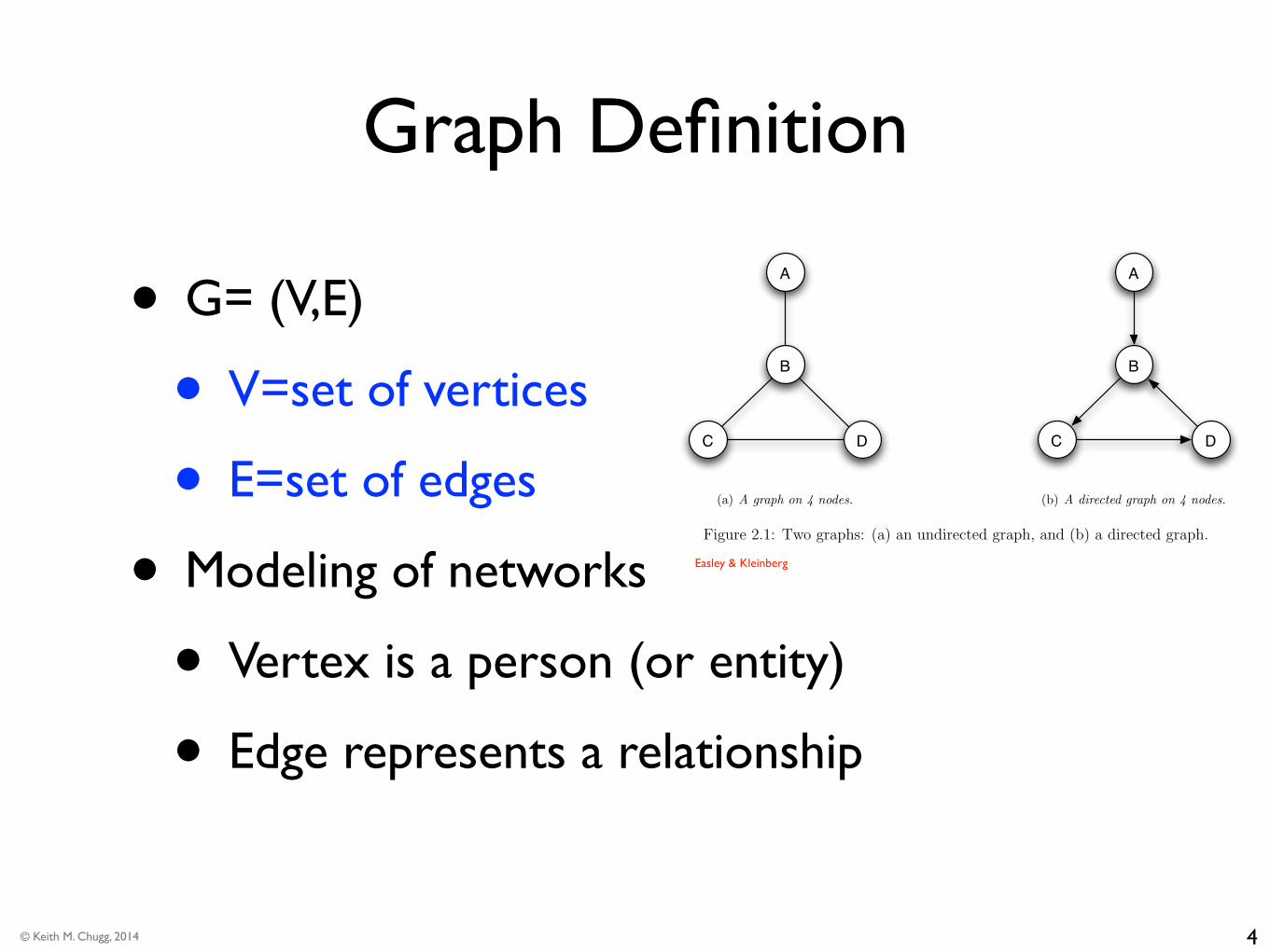
As with degree, we can compute statistical measures of distance

(empirical or analytical)


Figure 2.10: A histogram from Travers and Milgram’s paper on their small-world experiment[391]. For each possible length (labeled “number of intermediaries” on the x-axis), the plotshows the number of successfully completed chains of that length. In total, 64 chains reachedthe target person, with a median length of six.

such short paths, was a striking fact when it was first discovered, and it remains so today.

Of course, it is worth noting a few caveats about the experiment. First, it clearly doesn’t

establish a statement quite as bold as “six degrees of separation between us and everyone

else on this planet” — the paths were just to a single, fairly a✏uent target; many letters

never got there; and attempts to recreate the experiment have been problematic due to lack

of participation [255]. Second, one can ask how useful these short paths really are to people

in society: even if you can reach someone through a short chain of friends, is this useful to

you? Does it mean you’re truly socially “close” to them? Milgram himself mused about this

in his original paper [297]; his observation, paraphrased slightly, was that if we think of each

person as the center of their own social “world,” then “six short steps” becomes “six worlds

apart” — a change in perspective that makes six sound like a much larger number.

Despite these caveats, the experiment and the phenomena that it hints at have formed

a crucial aspect in our understanding of social networks. In the years since the initial

experiment, the overall conclusion has been accepted in a broad sense: social networks tend

to have very short paths between essentially arbitrary pairs of people. And even if your six-

Easley & Kleinberg


Distance Distribution

Easley & Kleinberg

2.3. DISTANCE AND BREADTH-FIRST SEARCH 37

Figure 2.11: The distribution of distances in the graph of all active Microsoft Instant Mes-senger user accounts, with an edge joining two users if they communicated at least onceduring a month-long observation period [273].

step connections to CEOs and political leaders don’t yield immediate payo↵s on an everyday

basis, the existence of all these short paths has substantial consequences for the potential

speed with which information, diseases, and other kinds of contagion can spread through

society, as well as for the potential access that the social network provides to opportunities

and to people with very di↵erent characteristics from one’s own. All these issues — and

their implications for the processes that take place in social networks — are rich enough

that we will devote Chapter 20 to a more detailed study of the small-world phenomenon and

its consequences.

Instant Messaging, Paul Erdos, and Kevin Bacon. One reason for the current em-

pirical consensus that social networks generally are “small worlds” is that this has been

increasingly confirmed in settings where we do have full data on the network structure. Mil-

gram was forced to resort to an experiment in which letters served as “tracers” through a

global friendship network that he had no hope of fully mapping on his own; but for other

kinds of social network data where the full graph structure is known, one can just load it

into a computer and perform the breadth-first search procedure to determine what typical


Small World Phenomena

http://www.ams.org/mathscinet/collaborationDistance.html

http://www.ams.org/mathscinet/collaborationDistance.html


Adjacency Matrix

N x N matrix A with

aij =

(1 (i, j) is edge

0 else

1 2

3 4

A =

2

664

0 1 1 01 0 0 11 0 0 10 1 1 0

3

775

captures all info about graph

discussed thus far


Adjacency Matrix=

⎛

⎝

⎜⎜⎜⎜⎜

⎞

⎠

⎟⎟⎟⎟⎟

A

A A A AA A A AA A A AA A A A

ij

11 12 13 14

21 22 23 24

31 32 33 34

41 42 43 44

=

⎛

⎝

⎜⎜⎜⎜

⎞

⎠

⎟⎟⎟⎟

A0 1 1 01 0 1 11 1 0 00 1 0 0

ij =

⎛

⎝

⎜⎜⎜⎜

⎞

⎠

⎟⎟⎟⎟

A0 0 1 01 0 1 00 0 0 00 1 0 0

ij

∑ ∑= = == =

k A A 3jj

ii

2 21

4

21

4

∑= ==

k A 2inj

j2 2

1

4

∑= ==

k A 1outi

i2 2

1

4

"A Aij ji "A 0ii |A Aij ji "A 0ii

∑==

L A12 ij

i j

N

, 1"k LN2 ∑=

=L Aij

i j

N

, 1" "k k L

Nin out

Image 2.7The adjacency matrix.

Top: The elements of the adjacency matrix. The adjacency matrix of a directed (left column) and an undirected (right column) network. The figure high-lights the fact that the degree of a node (in this case node 2) can be expressed as the sum over the appropriate column or row of the adjacency matrix. It also shows a few basic network characteristics, like the total number of links, (L), and average degree, (‹k›), expressed in terms of the elements of the adjacency matrix.

Adjacency matrix

Undirected network Directed network1

3 2

4

1

3 2

4

1

3 2

4

1

3 2

4


Baraba’si

degree info


Adjacency Matrix

Baraba’si

connectedness

SECTION 9

CONNECTEDNESS AND COMPONENTS

The phone would be of limited use as a communication device if we could not call any valid phone number; the email world be rather useless if we could send emails to only certain email addresses, and not to others. From a network perspective this means that the technology behind the phone or the Internet must be capable of establishing a path between any two devices or clients, like your phone and any other phone on the network or between yours and your acquaintance’s email address. This is in fact the key utility of most networks: they are built to ensure connect-edness. In this section we discuss the graph-theoretic for-mulation of connectedness.

In an undirected network two nodes i and j are connected if there is a path between them on the graph. They are dis-connected if such a path does not exist, in which case we have dij = ∞. This is illustrated in Image 2.14a, which shows

a network consisting of two disconnected clusters. While there are paths between the nodes that belong to the same cluster (for example nodes 4 and 6), there are no paths be-tween nodes that belong to different clusters (for example nodes 1 and 6).

A network is connected if all pairs of nodes in the network are connected. It is disconnected if there is at least one pair with dij = ∞. Clearly the network shown in Image 2.6a is disconnected, and we call its two subnetwork components (or clusters). A component is a subset of nodes in a net-work, so that there is a path between any two nodes that belong to the component, but one cannot add any more nodes to it that would have the same property. If a network consists of two components, a properly placed single link can connect them, making the network connected (Image 2.14b). Such a link is called a bridge. In general a bridge is any link that, if cut, disconnects the graph.

While for a small network visual inspection can help us decide if it is connected or disconnected, for a network consisting of millions of nodes connectedness is a chal-lenging question. Several mathematical tools help us iden-tify the connected components of a graph:

For a disconnected network the adjacency matrix can be rearranged into a block diagonal form, such that all nonzero elements in the matrix are contained in square blocks along the matrix’ diagonal and all other elements are zero (Image 2.14a). Each square block will correspond to a component. We can use the tools of linear algebra to decide if the adjacency matrix is block diagonal, helping us to identify the connected components.

In practice, for large networks the components are more efficient identified using the breadth first search algorithm (Box 2.7).

Image 2.14Connected and disconnected networks.

(a) The network consists of two disconnected components, i.e. there is a path between any pair of nodes in the (1,2,3) component, as well in the (4,5,6,7) component. However, there are no paths between nodes that belong to different connected components. The right panel shows the adjacently matrix of the network. If the network consists of disconnected components, the adjacency matrix can be rearranged into a block diagonal form, such that all nonzero elements of the matrix are contained in square blocks along the diagonal of the matrix and all other elements are zero.

(b) The addition of one link, called a bridge, can turn a disconnected network into a single connected component. Now there is a path between every pair of nodes in the network. Consequently the adjacency matrix cannot be written in a block diagonal form.

CONNECTEDNESS AND COMPONENTS | 39

node 4 is a “bridge”


Adjacency Matrix

Baraba’si

1 2

3 4

A =

2

664

0 1 1 01 0 0 11 0 0 10 1 1 0

3

775

A2 =

2

664

2 0 0 20 2 2 00 2 2 02 0 0 2

3

775

A3 =

2

664

0 4 4 04 0 0 44 0 0 40 4 4 0

3

775

1-hop connectivity

2-hop connectivity

3-hop connectivity

A = S⇤S�1

Ak = S⇤kS�1


Distance by BFS

• Breadth first search:

• Grow a tree from a given node, expanding outward

• Increment hop-count at each expansion step

• Disregard previously encountered nodes

!

• Advantage (potential)

• Matrix multiplication complexity ~ N*N

• BFS complexity ~ N+L (L=number of edges)


Distance by BFS26 CHAPTER 2. GRAPHS

LINC

CASE

CARN

HARV

BBN

MIT

SDC

RAND

UTAHSRI

UCLA

STANUCSB



























Easley & Kleinberg


LINC

CASE

CARN

HARV

BBN

MIT

SDC RAND

UTAH

SRI

UCLASTANUCSB

distance 1

distance 2

distance 3

Figure 2.9: The layers arising from a breadth-first of the December 1970 Arpanet, startingat the node mit.

really needed to trace out distances in the global friendship network (and had the unlimited

patience and cooperation of everyone in the world). This is pictured in Figure 2.8:

(1) You first declare all of your actual friends to be at distance 1.

(2) You then find all of their friends (not counting people who are already friends of yours),

and declare these to be at distance 2.

(3) Then you find all of their friends (again, not counting people who you’ve already found

at distances 1 and 2) and declare these to be at distance 3.

(...) Continuing in this way, you search in successive layers, each representing the next

distance out. Each new layer is built from all those nodes that (i) have not already

been discovered in earlier layers, and that (ii) have an edge to some node in the previous

layer.

This technique is called breadth-first search, since it searches the graph outward from a start-

ing node, reaching the closest nodes first. In addition to providing a method of determining

distances, it can also serve as a useful conceptual framework to organize the structure of a

graph, arranging the nodes based on their distances from a fixed starting point.


Distance by BFSImage 2.13The BFS algo-rithm applied to a small network.

Starting from the orange node, labeled ”0”, we identify all its neighbors, label-ing them ”1”. Then we label ”2” the un-labeled neighbors of all nodes labeled ”1”, and so on, in each iteration increasing the labels, until no node is left unla-beled. The length of the shortest path or the distance d0i between node 0 and some other node i in the network is given by the label on node i. For example, the distance between node 0 and the leftmost node is d03 = 3.


Baraba’si


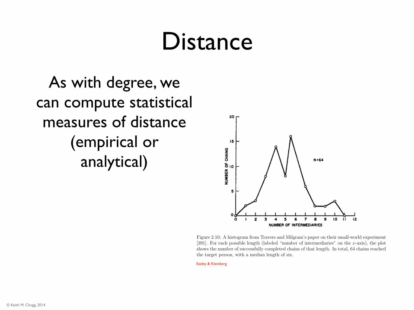
Summary & Extensions

Baraba’si

WEIGHTED NETWORK: a network whose links have a predefined weight, strength or fow parameter. The elements of the adjacency matrix are Aij = 0 if i and j are not connected, or Aij = wij if there is a link with weight wij between them. For unweighted (binary) networks, the adjacency matrix only indicates the presence (Aij = 1) or the absence (Aij = 0) of a link be-tween two nodes. Examples: Mobile phone calls, email network.

SELF-INTERACTIONS: in many networks nodes do not interact with themselves, so the diagonal elements of adjacency matrix are zero, Aii = 0, i =1,...,N. In some systems self-interactions are allowed; in such networks, representing the fact that node i has a self-interaction. Examples: WWW, protein interactions.

MULTIGRAPH: in a multigraph nodes are permitted to have multiple links (or parallel links) between them. Hence Aii can have any positive integer.

COMPLETE GRAPH: in a complete graph all nodes are connected to each other; no self-connections.

Image 2.16

Graphology.

In network science we encounter many networks distinguished by some elementary property of the underlying graph. Here we summarize the most commonly encountered elementary network types, together with their basic properties, and an illustrative list of real systems that share the particular property. Note that in many real network we need to combine several of these elementary network characteristics. For example the WWW is a directed multi-graph with self-interactions. The mobile call network is directed and weighted, without self-loops.

DIRECTED NETWORK: a network whose links have selected directions. Examples: WWW, mobile phone calls, citation network.

UNDIRECTED NETWORK: a network whose links do not have a predefined direction. Examples: Internet, power grid, science collaboration networks, protein interactions.

CASE STUDY AND SUMMARY | 43

Documents

Graph Theory and Social Networks - part I