GRAPH SPECTRAL ANALYSIS OF VOXEL-WISE BRAIN GRAPHSFROM DIFFUSION-WEIGHTED MRI

Anjali Tarun1,2, David Abramian3,4, Hamid Behjat5, Dimitri Van De Ville1,2

1 Institute of Bioengineering, Ecole Polytechnique Federale de Lausanne (EPFL), Switzerland2 Department of Radiology and Medical Informatics, University of Geneva (UNIGE), Switzerland

3 Department of Biomedical Engineering, University of Linkping, Sweden4 Center for Medical Image Science and Visualization, University of Linkping, Sweden

5 Department of Biomedical Engineering, Lund University, Lund, Sweden

ABSTRACT

Non-invasive characterization of brain structure has beenmade possible by the introduction of magnetic resonanceimaging (MRI). Graph modeling of structural connectivityhas been useful, but is often limited to defining nodes asregions from a brain atlas. Here, we propose two methodsfor encoding structural connectivity in a huge brain graphat the voxel-level resolution (i.e., 850’000 voxels) based ondiffusion tensor imaging (DTI) and the orientation densityfunctions (ODF), respectively. The eigendecomposition ofthe brain graph’s Laplacian operator is then showing highly-resolved eigenmodes that reflect distributed structural fea-tures which are in good correspondence with major whitematter tracks. To investigate the intrinsic dimensionality ofeigenspace across subjects, we used a Procrustes validationthat characterizes inter-subject variability. We found that theODF approach using 3-neighborhood captures the most in-formation from the diffusion-weighted MRI. The proposedmethods open a wide range of possibilities for new researchavenues, especially in the field of graph signal processingapplied to functional brain imaging.

Index Terms— brain graph, eigenmodes, diffusion tensorimaging, orientation density functions

1. INTRODUCTION

Diffusion-weighted magnetic resonance imaging (DW-MRI)allows for in vivo visualization of the diffusion of watermolecules in neural fibers, thereby revealing the underlyingbrain structure. Conventionally, various signal reconstructiontechniques as well as tractography algorithms [1, 2] are usedto derive white matter streamlines that connect the differentcortical and subcortical regions of the brain [3].

Viewed under the lens of graph theoretical approaches,distinct brain regions are usually represented as graph ver-tices. The graph edges and their associated weights encodethe strength of the association among regions [4–9], eitherbased on physical strength of the connections or the degree oftheir functional interplay. Whether it is a functional or struc-tural graph, one often limits the study in region-wise analysis

by averaging the neural activity or the number of fibers con-necting brain regions that are specified by an a priori atlas.Two limitations can be seen in such analysis. First, the analy-sis is drastically affected by the choice of parcellation scheme.It also merely provides a macro-scale view of structural orfunctional connectivity. Second, the analysis on structuralbrain graphs varies depending on the algorithm employed toapproximate the number of white matter (WM) tracts, andwhile they do reconstruct tractograms that are present, most ofthem also produce a significant amount of false positives [11].

In order to overcome these limitations, we propose tobuild a brain graph that is defined at a voxel-level resolu-tion. Doing so would not require the use of any parcellationschemes and tractography algorithms, and instead built di-rectly from the reconstructed diffusion data. We present twodesign schemes, one using DTI data and the other using ODFdata. The ODF design is explored using two levels of neig-borhood connectivity principle, namely, 3 and 5 connectivityin 3D. We show, for the first time, highly resolved humanbrain eigenmodes that recover major white matter tracks. TheLaplacian spectra of the resulting graphs are compared todetermine which design maximally encodes diffusion data.

2. METHODS

Similar to classical brain graphs, we define a brain graph asGvw := (V,A), where V = {1, 2, 3, ...,N } is the set of Nnodes representing the brain voxels, and A ∈ N × N is anadjacency matrix encoding the connection strength betweenneighboring voxels. The specific definition of neighboringvoxels depends on the type of signal reconstruction being con-sidered.

2.1. DTI-based brain graph

In DTI, the fiber orientation at a voxel is described by an el-lipsoid defined by a real symmetric 3 × 3 matrix T calledthe diffusion tensor. The displacement probability of watermolecules at a given time can then be approximated by a mul-tivariate Gaussian with the diffusion tensor as the covariance

2019 IEEE 16th International Symposium on Biomedical Imaging (ISBI 2019)Venice, Italy, April 8-11, 2019

978-1-5386-3640-4/19/$31.00 ©2019 IEEE 159

0.01 90

9 900

0.007 90

0.03

9

0.02

50 1000

500 1E+13

50 1000

50

500

50

0.02 90

9 900

0.003 90

0.07

9

0.01

�ij�=�4�/26

rj

ri

A B C

Fig. 1. (A) Filter coefficients obtained by discretizing the representative tensor shown; (B) adapts Itturia-Medina’s originalfigure [10] illustrating the solid angle βij around the vector rij , while (C) visualizes DTI data through ellipsoids, and thecorresponding voxel-wise brain graph (y = 87).

matrix, given by [12]:

P (�ri, ti) ==1√

4πti3|T|

exp(− �riTT−1�ri4t

), (1)

where �ri and ti translate to the direction at a specific voxeland timepoint being considered. We used a cubic lattice ofsize 3× 3× 3 Moore neighborhood to define the nodes of ourbrain graph, so that each node is connected up to a maximumof 26 nearest neighbors. The calculation of the equivalentweights requires a discretization step that guarantees a one-to-one mapping between the (continuous) multivariate Gaussianmodel and the (discrete) weighting of vertices in the braingraph. This is done by assigning a cubic FIR filter in eachvoxel, defined as h(k), and obtaining the filter coefficientsthat are equivalent to the diffusion ellipsoid that is modeled byEquation 1. We specify h(k) in terms of its transfer functionas

H(z) =∑k

h(k)z−k (2)

where zk is equivalent to∏i=M

i=1 zkii , with M = 3. The one

to one mapping from the continuous domain to the discretedomain is achieved by matching equations 1 and 2 in their re-spective frequency domain representation. Fundamental sig-nal processing concepts allow us to do the matching by not-ing that the Z-transform is essentially a discrete version of theFourier transform (FT) if we set the real part of the complexvariable to zero. Under the same frequency representation,we can expand in terms of their Taylor series approximation,and obtain the filter coefficients by matching the coefficientsof the lowest order terms. The filter coefficients are normal-ized in each voxel and are multiplied with the correspond-ing fractional anisotropy (FA) in order to boost the structureof the graph. For each voxel i in the brain, we encode the

discrete counterpart of the diffusion ellipsoid onto the braingraph, noting that Ai,j is given by the average of two coincid-ing filter coefficients coming from voxels i and j. An exampleof a discretized ellipsoid is shown in Fig. 1(A) and a visual-ization of DTI ellipsoids and their corresponding voxel-wisebrain graph for a representative coronal slice in Fig. 1(C).

2.2. ODF-based brain graph

We used an ODF-based weighting scheme that leverages pre-vious work presented by Itturia-Medina [10, 13]. Let Ni de-note the set of vertices in V that are adjacent to vertex i. Forany two vertices i, j ∈ V , let �rij denote the vector pointingfrom the center of vertex i to the center of vertex j. Let Oi(S)denote the ODF associated to voxel ri, with its center of co-ordinate being the center of the voxel. We can then define

p(i, �rij) =

∫βij

Oni (S)dS (3)

as the probability of the nerve fibers being oriented alongdirection �rij . The variable n is a positive integer that is adesired power factor to sharpen the ODFs, and βij denotesa solid angle of 4π/98 (for 5-neighborhood, 4π/26 for 3-neighborhood) around �rij subtended at the center of voxelri (see Fig. 1(B)). Let {Oi,k}No

k=1 denote the discrete samplesof Oi(S) along No directions {�rk}No

k=1 from the center of theODF. Thus, p(i, �rij) can instead be approximated as a sum

p(i, �rij) ≈ 4π

No

∑k∈Di,j

Oni,k, (4)

where Di,j : {k | �rk ∈ βij}. The final weights of the braingraph are computed by taking into account the strength of theanisotropy of the nodes ri and rj and the ODF’s orientation

160

DTI - 3

ODF - 3

ODF - 5

Eigenmode 1 Eigenmode 2 Eigenmode 3

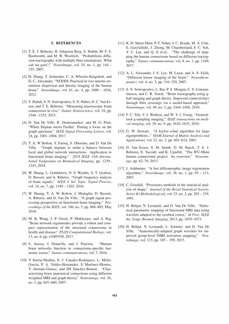
Fig. 2. Human brain eigenmodes of a representative subject corresponding to the top 3 lowest frequencies, produced by braingraphs constructed using 3-neighborhood DTI and 3 and 5-neighborhood ODF.

p(i, �rij). Mathematically,

Ai,j = Pmag(ri)p(i, �rij) + Pmag(rj)p(j, �rji) (5)

where Pmag(ri) is defined as

Pmag(ri) =QA2

2maxl∈Nkp(k, �rkl)

(6)

where QA is the anisotropy index called the quantitativeanisotropy that is originally defined by Yeh et. al [14], and thedenominator is a normalization term for p(i, �rij). WhereasItturia-Medina [10] has defined a parameter based on tissueprobability maps to describe the magnitude of the anatomicalinformation, we propose to use QA, synonymous to FA inDTI. In particular, ODF provides the directionality (shape) ofthe diffusion, while the squared QA provides the magnitude(energy). By nature of the design of the ODF brain graph, wecan choose to use a 3 × 3 × 3 or a 5 × 5 × 5 neighborhood,depending on the solid angle β that we consider. The 5-neighborhood intuitively offers a more resolved connectivityinformation, whereas the 3-neighborhood is more localized.

3. RESULTS

We constructed and evaluated three different brain graphs: (i)the 3-neighborhood DTI-based (DTI-3), (ii) the 3-neighborhoodODF-based (ODF-3) and (iii) the 5-neighborhood ODF-based(ODF-5) graph. A fourth graph with randomly assigned edgeweights, using a Gaussian noise, is constructed and treatedas a null for comparing and evaluating the brain graphs. Thebrain graphs are constructed within the native space wherediffusion data were acquired, and it includes all voxels from

all tissue types, i.e., gray matter (GM), white matter and thecerebrospinal fluid (CSF).

To capture the topology, we consider the graph Lapla-cian matrix in its symmetric normalized form Lsym =

D1/2LD1/2. The eigendecomposition of Lsym leads to acomplete set of orthonormal eigenvectors that span the graphspectral domain and of N real, non-negative eigenvalues.The number of nodes typically range around 700-900 thou-sand for the whole brain graph, and as such, the dimensionposes significant computational challenge. The present proof-of-concept analysis was therefore confined to the first 1000eigenvectors corresponding to the lowest spectral frequencies,estimated using the Krylov–Schur Algorithm [15].

The diffusion is inherently anisotropic in the WM in con-trast to being isotropic in GM and CSF. This is reflected inFig. 2 which illustrates the first three eigenmodes of the threebrain graphs. Major WM structures clearly dominate theoverall spatial pattern, indicating that the distinction betweentissue types naturally arises from the assignment of the con-nectivity weights in the brain graph. The second and thirdeigenmodes show geometrical information of the head shape,dividing the brain into posterior and anterior, and left andright, respectively, while higher frequency eigenmodes showmore spatial variability and more localized information.

By nature of the reconstruction models, ODFs are ex-pected to recover more details, especially in crossings andbranching fibers. However, as it is shown in Fig. 2, it is noteasy to qualitatively pinpoint the differences of the approachthrough visual inspection. In order to characterize the differ-ences in their topology, we look at the general trend of theeigenmodes in a population of 20 subjects from the HumanConnectome Project (HCP) [16] database.

161

50 100 150 200 250 300Subject 1 Eigenmodes

-1

-0.8

-0.6

-0.4

-0.2

0

0.2

0.4

0.6

0.8

1

50 100 150 200 250 300Subject 1 Eigenmodes

50

100

150

200

250

300

Sub

ject

2 E

igen

mod

es

100 200 300 400 500 600 700 800 900 1000

Number of Eigenmodes (k)

0

0.4

0.8

1.2

1.6

Pro

crus

tes

Err

or

x 10-4

ODF 3ODF 5DTINull

A

B

Fig. 3. (A) Cosine similarity of the first 300 eigenmodesof two representative subjects before (left) and after (right)Procrustes transform, where we see traces of flipped signsand unordered eigenmodes before applying the transforma-tion. The curve in (B) summarizes the Procrustes error cal-culated by summing up off-diagonal values in all pair-wisecosine similarity matrices. The ODF-3 shows the highest pro-crustes error, while the DTI and ODF-5 tied for second.

3.1. Procrustes validation

If the application calls for a group-level analysis, normaliza-tion using DARTEL [17] is suggested so that the deformationtemplates are specific to the group being analyzed. Theeigendecomposition of the Laplacian returns subject-specificeigenmodes that are not necessarily in the same order withother subjects. To solve this, we used Procrustes trans-form [18] to flip the signs of the eigenmodes and re-orderthem accordingly. After an iterative Procrustes transforma-tion, we obtain an averaged set of human brain eigenmodesrepresentative of the population considered.

To examine the efficiency of the Procrustes transforma-tion, we applied a cosine similarity measure to all pair-wisecombination of subjects, see Fig. 3(A). Traces of flippedsigns and unordered eigenmodes are observed before Pro-crustes transformation. Each set of eigenmodes containssubject-specific structural information, and while the Pro-crustes transformation matches similar eigenmodes, it can-not account for inherent inter-subject variability. Therefore,off-diagonal errors in the similarity matrix reflect these dif-ferences. We ran bootstrap methods to successively applyProcrustes transformation on a subset of 15 out of the total of20 subjects. We examined the cosine similarity errors for in-creasing number of eigenmodes as is shown in Fig. 3(B). By

summing up all off-diagonal values in the cosine similaritymatrices, computed multiple times (with replacement) fromall 20 subjects, we computed an error term, denoted Pro-crustes error. We found all four graphs showing a decreasingL-curve, having knee-points at around k = 300 and reachingthat of the null upon reaching higher k-values, suggesting thatonly the top 300 eigenmodes show relevant structure. TheODF-3 graph shows the highest procrustes error, while theDTI-3 and and ODF-5 graphs tied on the second spot, sug-gesting that the ODF-3 graph recovered the highest amountof information from the diffusion data.

4. CONCLUSION

Two design schemes for constructing voxel-vise brain graphsbased on DTI and ODF were presented. The approach ex-tends a previously proposed brain graph design limited to theGM [19,20], and a modified and improved versions of Itturia-Medina’s ODF-based brain graph [10, 13]. The brain graphsare constructed within the native diffusion space and havenodes covering the entire brain, including GM, WM and CSF.Thus, there are no coordinate transformation nor segmenta-tion processes involved, making the brain graph more reliableand subject-specific. The decomposition of the Laplacianproduced highly resolved human brain eigenmodes show-ing structural features that are in good correspondence withknown major white matter bundles. Moreover, through a Pro-crustes validation scheme that is able to reflect inter-subjectdifferences, we found that the 3-neighborhood ODF-basedbrain graph is better than the DTI-based owing to the fact thatDTI is a much simpler model making it unable to reconstructfiber crossings and branching patterns. Furthermore, we sur-mise that although the 3-neighborhood and 5-neighborhoodODF come from the same reconstruction method, the use ofa higher-neighborhood scheme reduces the amount of infor-mation captured due to increased complexity and the possibleinclusion of distant connections.

From a neuroscience perspective, the introduction ofvoxel-wise brain graphs opens a wide-range of new possibil-ities for the study of the brain. In the structural perspectivealone, brain eigenmodes have been found as an effectivebiomarker for distinguishing healthy and diseased [8]. More-over, brain eigenmodes have also been introduced as a build-ing block for the human connectome [9] and cortical neuralactivity can be decomposed into frequency-specific modes.Similar to this, our method has the potential to extend theexploration not only in the cortex, but in the whole brain ata very high resolution. With the rising use of graph signalprocessing (GSP) in the field [5–7], this approach can propelstudies aiming to understand how the dynamics of neuralprocesses relate to the underlying fixed anatomical structure.The key is to define the functional data as signals residingin the voxel-wise brain grid, so that various GSP operations(e.g., filtering, signal inpainting) can then be tailored andexplored according to the research question.

162

5. REFERENCES

[1] T. E. J. Behrens, H. Johansen Berg, S. Jbabdi, M. F. S.Rushworth, and M. W. Woolrich, “Probabilistic diffu-sion tractography with multiple fibre orientations: Whatcan we gain?,” NeuroImage, vol. 34, no. 1, pp. 144 –155, 2007.

[2] H. Zhang, T. Schneider, C. A. Wheeler-Kingshott, andD. C. Alexander, “NODDI: Practical in vivo neurite ori-entation dispersion and density imaging of the humanbrain,” NeuroImage, vol. 61, no. 4, pp. 1000 – 1016,2012.

[3] S. Jbabdi, S. N. Sotiropoulos, S. N. Haber, D. C. Van Es-sen, and T. E. Behrens, “Measuring macroscopic brainconnections in vivo,” Nature Neuroscience, vol. 18, pp.1546 –1555, 2015.

[4] D. Van De Ville, R. Demesmaeker, and M. G. Preti,“When Slepian meets Fiedler: Putting a focus on thegraph spectrum,” IEEE Signal Processing Letters, vol.24, pp. 1001–1004, 2017.

[5] T. A. W Bolton, Y. Farouj, S. Obertino, and D. Van DeVille, “Graph slepians to strike a balance betweenlocal and global network interactions: Application tofunctional brain imaging,” 2018 IEEE 15th Interna-tional Symposium on Biomedical Imaging, pp. 1239–1243, 2018.

[6] W. Huang, L. Goldsberry, N. F. Wymbs, S. T. Grafton,D. Bassett, and A. Ribeiro, “Graph frequency analysisof brain signals,” IEEE J. Sel. Topic. Signal Process,vol. 10, no. 7, pp. 1189 – 1203, 2016.

[7] W. Huang, T. A. W. Bolton, J. Medaglia, D. Bassett,A. Ribeiro, and D. Van De Ville, “A graph signal pro-cessing perspective on functional brain imaging,” Pro-ceedings of the IEEE, vol. 106, no. 5, pp. 868–885, May2018.

[8] M. B. Wang, J. P. Owen, P. Mukherjee, and A. Raj,“Brain network eigenmodes provide a robust and com-pact representation of the structural connectome inhealth and disease,” PLOS Computational Biology, vol.13, no. 6, pp. e1005550, 2017.

[9] S. Atasoy, I. Donnelly, and J. Pearson, “Humanbrain networks function in connectome-specific har-monic waves,” Nature communications, vol. 7, 2016.

[10] Y Iturria-Medina, E. J. Canales-Rodriguez, L. Melie-Garcia, P. A. Valdes-Hernandez, E Martinez-Montes,Y Aleman-Gomez, and JM Sanchez-Bornot, “Char-acterizing brain anatomical connections using diffusionweighted MRI and graph theory,” Neuroimage, vol. 36,no. 3, pp. 645–660, 2007.

[11] K. H. Maier-Hein, P. F. Neher, J. C. Houde, M. A. Cote,E. Garyfallidis, J. Zhong, M. Chamberland, F. C. Yeh,Y. C. Lin, and Q. Ji et.al., “The challenge of map-ping the human connectome based on diffusion tractog-raphy,” Nature communications, vol. 8, no. 1, pp. 1349,2017.

[12] A. L. Alexander, J. E. Lee, M. Lazar, and A. S. Field,“Diffusion tensor imaging of the brain,” Neurothera-peutics, vol. 4, no. 3, pp. 316–329, 2007.

[13] S. N. Sotiropoulos, L. Bai, P. S. Morgan, C. S. Constan-tinescu, and C. R. Tench, “Brain tractography using q-ball imaging and graph theory: Improved connectivitiesthrough fibre crossings via a model-based approach,”Neuroimage, vol. 49, no. 3, pp. 2444–2456, 2010.

[14] F. C. Yeh, V. J. Wedeen, and W. Y. I. Tseng, “General-ized q-sampling imaging,” IEEE transactions on medi-cal imaging, vol. 29, no. 9, pp. 1626–1635, 2010.

[15] G. W. Stewart, “A krylov-schur algorithm for largeeigenproblems.,” SIAM Journal of Matrix Analysis andApplications, vol. 23, no. 3, pp. 601–614, 2001.

[16] D. Van Essen, S. M. Smith, D. M. Barch, T. E. J.Behrens, E. Yacoub, and K. Ugurbil, “The WU-Minnhuman connectome project: An overview,” Neuroim-age, pp. 62–79, 2013.

[17] J. Ashburner, “A fast diffeomorphic image registrationalgorithm,” NeuroImage, vol. 38, no. 1, pp. 95 – 113,2007.

[18] C. Goodall, “Procrustes methods in the statistical anal-ysis of shape,” Journal of the Royal Statistical Society.Series B (Methodological), vol. 53, no. 2, pp. 285 – 339,1991.

[19] H. Behjat, N. Leonardi, and D. Van De Ville, “Statis-tical parametric mapping of functional MRI data usingwavelets adapted to the cerebral cortex,” in Proc. IEEEInt. Symp. Biomed. Imaging, 2013, pp. 1070–1073.

[20] H. Behjat, N. Leonardi, L. Sornmo, and D. Van DeVille, “Anatomically-adapted graph wavelets for im-proved group-level fMRI activation mapping,” Neu-roImage, vol. 123, pp. 185 – 199, 2015.

163