1

Graph Laplacian Tomography from Unknown

Random ProjectionsRonald. R. Coifman, Yoel Shkolnisky, Fred J. Sigworth and Amit Singer

Abstract—We introduce a graph Laplacian based algorithmfor the tomography reconstruction of a planar object from itsprojections taken at random unknown directions. The algorithmis shown to successfully reconstruct the Shepp-Logan phantomfrom its noisy projections. Such a reconstruction algorithm isdesirable for the structuring of certain biological proteins usingcryo electron microscopy.

I. INTRODUCTION

A standard problem in computerized tomography (CT)

is reconstructing an object from samples of its projections.

Focusing our attention to a planar object characterized by its

density function ρ(x, y), its Radon transform projection Pθ(t)

is the line integral of ρ along parallel lines L inclined at an

angle θ with distances t from the origin (see, e.g, [1]–[3])

Pθ(t) =∫

L

ρ(x, y)ds

=∫∫ ∞

−∞ρ(x, y)δ(x cos θ + y sin θ − t)dx dy.

(1)

The function ρ represents a property of the examined object

which depends on the imaging modality. For example, ρ

represents the X-ray attenuation coefficient in the case of X-

ray tomography (CT scanning), the concentration of some

radioactive isotope in PET scanning, or the refractive index

of the object in ultrasound tomography.

Tomographic reconstruction algorithms estimate the func-

tion ρ from a finite set of samples of Pθ(t), assuming that

Ronald R. Coifman, Yoel Shkolnisky and Amit Singer are with the Depart-

ment of Mathematics, Program in Applied Mathematics, Yale University, 10

Hillhouse Ave. PO Box 208283, New Haven, CT 06520-8283 USA.

Fred J. Sigworth is with the Department of Cellular and Molecular Phys-

iology, Yale University School of Medicine, 333 Cedar Street, New Haven,

CT 06520 USA.

emails: coifman-ronald@yale.edu, yoel.shkolnisky@yale.edu,

fred.sigworth@yale.edu, amit.singer@yale.edu

the sampling points (θ, t) are known. See [4] for a sur-

vey of tomographic reconstruction methods. However, there

are cases in which the projection angles are unknown, for

example, when reconstructing certain biological proteins or

other moving objects. In such cases, one is given samples

of the projection function Pθi(t) for a finite but unknown

set of angles {θi}, and the problem at hand is to estimate

the underlying function ρ without knowing the angle values.

The sampling set for the parameter t is usually known and

dictated by the physical setting of the acquisition process; for

example, if the detectors are equally spaced then the values of

t correspond to the location of the detectors along the detectors

line, while the origin may be set at the center of mass.

In this paper we consider the reconstruction problem for

the 2D parallel-beam model with unknown acquisition angles.

Formally, we consider the following problem: Given N projec-

tion vectors (Pθi(t1), Pθi(t2), . . . , Pθi(tn)) taken at unknown

angles {θi}Ni=1 that were randomly drawn from the uniform

distribution of [0, 2π] and t1, t2, . . . , tn are fixed n equally

spaced pixels in t, find the underlying density function ρ(x, y)

of the object.

A solution to this problem based on the moments of the

projections was suggested and analyzed in [5], [6], where

a simpler symmetric nearest neighbor algorithm was also

described and tested numerically. Estimation of the projection

angles is obtained from their ordering. This follows from

the properties of the order statistics of uniformly distributed

angles. Once the ordering is determined, the projection angles

are estimated to be equally spaced on the unit circle. Thus,

the problem boils down to sorting the projections with respect

to their angles.

Our proposed algorithm sorts the projections by using

the graph Laplacian [7], [8]. Graph Laplacians are widely

2

used in machine learning for dimensionality reduction, semi-

supervised learning and spectral clustering. However, their

application to this image reconstruction problem seems to be

new. Briefly speaking, an N by N matrix of weights related to

the pairwise projection distances is constructed, followed by

a computation of its first few eigenvectors. The eigenvectors

reveal the correct ordering of the projections in a manner to

be later explained. This algorithm may also be viewed as a

generalization of the nearest-neighbor insertion algorithm [6]

as it uses several weighted nearest neighbors at once. More

importantly, the graph Laplacian incorporates all local pieces

of information into a coherent global picture, eliminating

the dependence of the outcome on any single local datum.

Small local perturbations of the data points have almost no

effect on the outcome. This global information is encoded in

the first few smooth and slowly-varying eigenvectors, which

depend on the entire dataset. Our numerical examples show

that increasing the number of projections improves the perfor-

mance of the sorting algorithm. We examine the influence of

corrupting the projections by white Gaussian additive noise on

the performance of the graph Laplacian sorting algorithm and

its ability to reconstruct the underlying object. We find that

applying classical filtering methods to de-noise the projection

vectors, such as the translation invariant spin-cycle wavelet

de-noising [9], gives successful reconstructions at even higher

levels of noise.

This work was motivated by a similar problem in three

dimensions, where a 3D object is to be reconstructed from

its 2D line integral projections (X-ray transform) taken at

unknown directions, as is the case in CryoEM microscopy

[10]–[12]. Though there is no sense of order anymore, the

graph Laplacian may be used to reveal the projection directions

also in this higher dimensional case, as will be described in

further details in a separate publication.

The organization of the paper is as follows. In Section II we

survey graph Laplacians, which are being used in Section III

for solving the tomography problem. The performance of the

algorithm is demonstrated in Section IV. Finally, Section V

contains some concluding remarks and a discussion of future

extensions.

II. GRAPH LAPLACIANS SORT PROJECTIONS

Though graph Laplacians are widely used in machine learn-

ing for dimensionality reduction of high dimensional data,

semi-supervised learning and spectral clustering, their usage

in tomography is uncommon. For that reason, a self contained

albeit limited description of graph Laplacians is included here.

The presentation alternates between a general presentation of

graph Laplacians and a specific consideration of their role

in the tomography problem at hand. For a more detailed

description of graph Laplacians and their applications the

reader is referred to [7], [8], [13]–[15] (and references therein).

A. Spectral embedding

In the context of dimensionality reduction, high dimensional

data points are described by a large number of coordinates n,

and a reduced representation that uses only a few effective co-

ordinates is wanted. Such a low-dimensional representation is

sought to preserve properties of the high-dimensional dataset,

such as, local neighborhoods [13], [16], geodesic distances

[17] and diffusion distances [7]. It is often assumed that the

data points approximately lie on a low dimensional manifold,

typically a non-linear one. In such a setting, the N data points

x1, . . . , xN are viewed as points in the ambient Euclidean

space Rn, while it is assumed that they are restricted to

an intrinsic low dimensional manifold M. In other words,

x1, . . . , xN ∈ M ⊂ Rn and d = dimM ¿ n. We assume

that the structure of the manifold M is unknown, and one can

only access the data points x1, . . . , xN as points in Rn. Fitting

the data points using linear methods such as linear regression,

least square approximation or principal component analysis, to

name a few, usually performs poorly when the manifold is non-

linear. The graph Laplacian, however, is a non-linear method

that overcomes the shortcomings of the linear methods.

In our tomography problem, each data point corresponds

to a projection at some fixed angle θi, sampled at n equally

spaced points in the t direction

xi = (Pθi(t1), Pθi(t2), . . . , Pθi(tn)) , i = 1, 2, . . . , N. (2)

The vector that corresponds to each projection is viewed as a

point xi ∈ Rn; however, all points xi lie on a closed curve

P ⊂ Rn where

P (θ) = (Pθ(t1), Pθ(t2), . . . , Pθ(tn)) , θ ∈ [0, 2π). (3)

3

The closed curve P is a one dimensional manifold of Rn

(d = 1) parameterized by the projection angle θ. The exact

shape of the curve depends on the underlying imaged object

ρ(x, y), so different objects give rise to different curves. The

particular curve P is unknown to us, because the object ρ(x, y)

is unknown. However, recovering the curve, or, in general,

the manifold, from a sufficiently large number of data points

sounds plausible.

In practice, the manifold is recovered by constructing the

graph Laplacian and computing its first few eigenvectors. The

starting point is constructing an N×N weight matrix W using

a suitable semi-positive kernel k as follows

Wij = k

(‖xi − xj‖22ε

), i, j = 1, . . . , N, (4)

where ‖·‖ is the Euclidean norm of the ambient space Rn and

ε > 0 is a parameter known as the bandwidth of the kernel.

A popular choice for the kernel function is k(x) = exp(−x),

though other choices are also possible [7], [8]. The weight

matrix W is then normalized to be row stochastic, by dividing

it by a diagonal matrix D whose elements are the row sums

of W

Dii =N∑

j=1

Wij . (5)

The (negative defined) normalized graph Laplacian L is then

given by

L = D−1W − I, (6)

where I is the N × N identity matrix. There exist nor-

malizations other than the row stochastic one; the choice of

normalization and the differences between them are addressed

below.

The row stochastic matrix D−1W has a complete set of

eigenvectors φi and eigenvalues λi

1 = λ0 > λ1 ≥ . . . ≥ λi ≥ λi+1 ≥ . . . ≥ λN−1 ≥ 0,

and the first eigenvector is constant, that is, φ0 =

(1, 1, . . . , 1)T . The remaining eigenvectors φ1, . . . , φk, for

some k ¿ N , define a k-dimensional non-linear spectral

embedding of the data

xi 7→ (φ1(i), φ2(i), . . . , φk(i)) , i = 1, . . . , N. (7)

It is sometimes advantageous to incorporate the eigenvalues

into the embedding by defining

xi 7→(λt

1φ1(i), λt2φ2(i), . . . , λt

kφk(i)), i = 1, . . . , N,

for some t ≥ 0 [7].

B. Uniform datasets and the Laplace-Beltrami operator

The embedding (7) has many nice properties and we choose

to emphasize only one of them, namely the intimate connec-

tion between the graph Laplacian matrix L and the continuous

Laplace-Beltrami operator ∆M of the manifold M. This

connection is manifested in the following theorem [18]: if

the data points x1, x2, . . . , xN are independently uniformly

distributed over the manifold M then with high probability

1ε

N∑

j=1

Lijf(xj) =12∆Mf(xi)+O

(1

N1/2ε1/2+d/4, ε

), (8)

where f : M 7→ R is any smooth function. The approxi-

mation in (8) incorporates two error terms: a bias term of

O(ε) which is independent of N and a variance term of

O(N−1/2ε−(1/2+d/4)

). The theorem implies that the discrete

operator L converges pointwise to the continuous Laplace-

Betrami operator in the limit ε → 0 and N → ∞ as long as

Nε1+d/2 →∞.

In other words, applying the discrete operator L to a

smooth function sampled at the data points approximates

the Laplace-Beltrami of that function evaluated at those data

points. Moreover, the eigenvectors of the graph Laplacian L

approximate the eigenfunctions of ∆M that correspond to

homogenous Neumann boundary condition (vanishing normal

derivative) in the case that the manifold has a boundary [19].

This connection between the graph Laplacian and the

Laplace-Beltrami operator sheds light on the spectral embed-

ding (7). For example, consider a closed curve P ⊂ Rn

of length L parameterized by its arclength s. The Laplace-

Beltrami ∆P of P is simply the second order derivative with

respect to the arclength, ∆P f(s) = f ′′(s). The eigenfunctions

of ∆P satisfy

f ′′(s) = −λf(s), s ∈ (0, L) (9)

with the periodic boundary conditions

f(0) = f(L), f ′(0) = f ′(L). (10)

4

−1 −0.5 0 0.5 1

−1

−0.5

0

0.5

1

x

y

(a)

−1 −0.5 0 0.5 1

−1

−0.5

0

0.5

1

φ1

φ 2

(b)

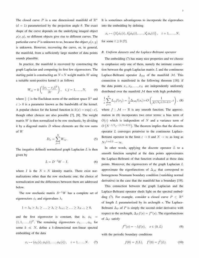
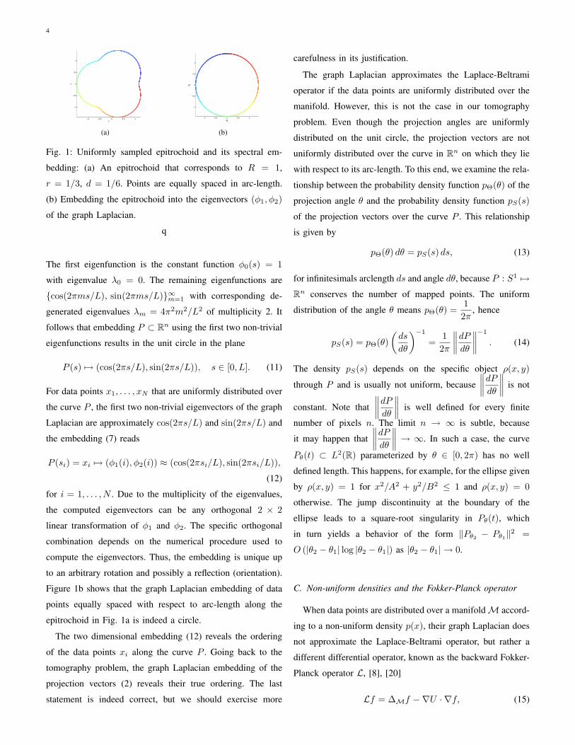
Fig. 1: Uniformly sampled epitrochoid and its spectral em-

bedding: (a) An epitrochoid that corresponds to R = 1,

r = 1/3, d = 1/6. Points are equally spaced in arc-length.

(b) Embedding the epitrochoid into the eigenvectors (φ1, φ2)

of the graph Laplacian.

q

The first eigenfunction is the constant function φ0(s) = 1

with eigenvalue λ0 = 0. The remaining eigenfunctions are

{cos(2πms/L), sin(2πms/L)}∞m=1 with corresponding de-

generated eigenvalues λm = 4π2m2/L2 of multiplicity 2. It

follows that embedding P ⊂ Rn using the first two non-trivial

eigenfunctions results in the unit circle in the plane

P (s) 7→ (cos(2πs/L), sin(2πs/L)), s ∈ [0, L]. (11)

For data points x1, . . . , xN that are uniformly distributed over

the curve P , the first two non-trivial eigenvectors of the graph

Laplacian are approximately cos(2πs/L) and sin(2πs/L) and

the embedding (7) reads

P (si) = xi 7→ (φ1(i), φ2(i)) ≈ (cos(2πsi/L), sin(2πsi/L)),

(12)

for i = 1, . . . , N . Due to the multiplicity of the eigenvalues,

the computed eigenvectors can be any orthogonal 2 × 2

linear transformation of φ1 and φ2. The specific orthogonal

combination depends on the numerical procedure used to

compute the eigenvectors. Thus, the embedding is unique up

to an arbitrary rotation and possibly a reflection (orientation).

Figure 1b shows that the graph Laplacian embedding of data

points equally spaced with respect to arc-length along the

epitrochoid in Fig. 1a is indeed a circle.

The two dimensional embedding (12) reveals the ordering

of the data points xi along the curve P . Going back to the

tomography problem, the graph Laplacian embedding of the

projection vectors (2) reveals their true ordering. The last

statement is indeed correct, but we should exercise more

carefulness in its justification.

The graph Laplacian approximates the Laplace-Beltrami

operator if the data points are uniformly distributed over the

manifold. However, this is not the case in our tomography

problem. Even though the projection angles are uniformly

distributed on the unit circle, the projection vectors are not

uniformly distributed over the curve in Rn on which they lie

with respect to its arc-length. To this end, we examine the rela-

tionship between the probability density function pΘ(θ) of the

projection angle θ and the probability density function pS(s)

of the projection vectors over the curve P . This relationship

is given by

pΘ(θ) dθ = pS(s) ds, (13)

for infinitesimals arclength ds and angle dθ, because P : S1 7→Rn conserves the number of mapped points. The uniform

distribution of the angle θ means pΘ(θ) =12π

, hence

pS(s) = pΘ(θ)(

ds

dθ

)−1

=12π

∥∥∥∥dP

dθ

∥∥∥∥−1

. (14)

The density pS(s) depends on the specific object ρ(x, y)

through P and is usually not uniform, because∥∥∥∥

dP

dθ

∥∥∥∥ is not

constant. Note that∥∥∥∥

dP

dθ

∥∥∥∥ is well defined for every finite

number of pixels n. The limit n → ∞ is subtle, because

it may happen that∥∥∥∥

dP

dθ

∥∥∥∥ → ∞. In such a case, the curve

Pθ(t) ⊂ L2(R) parameterized by θ ∈ [0, 2π) has no well

defined length. This happens, for example, for the ellipse given

by ρ(x, y) = 1 for x2/A2 + y2/B2 ≤ 1 and ρ(x, y) = 0

otherwise. The jump discontinuity at the boundary of the

ellipse leads to a square-root singularity in Pθ(t), which

in turn yields a behavior of the form ‖Pθ2 − Pθ1‖2 =

O (|θ2 − θ1| log |θ2 − θ1|) as |θ2 − θ1| → 0.

C. Non-uniform densities and the Fokker-Planck operator

When data points are distributed over a manifold M accord-

ing to a non-uniform density p(x), their graph Laplacian does

not approximate the Laplace-Beltrami operator, but rather a

different differential operator, known as the backward Fokker-

Planck operator L, [8], [20]

Lf = ∆Mf −∇U · ∇f, (15)

5

where U(x) = −2 log p(x) is the potential function. Thus, the

more general form of (8) is

1ε

N∑

j=1

Lijf(xj) ≈ 12Lf(xi). (16)

Note that the Fokker-Planck operator L coincides with the

Laplace-Beltrami operator in the case of a uniform distribution

for which the potential function U is constant, so its gradient

vanishes.

The Fokker-Planck operator has a complete set of eigen-

functions and eigenvalues. In particular, when the manifold is

a closed curve P of length L, the eigenfunctions satisfy

f ′′ − U ′f ′ = −λf (17)

with the periodic boundary conditions

f(0) = f(L), f ′(0) = f ′(L). (18)

We rewrite the eigenfunction problem (17) as a Sturm-

Liouville problem

(e−Uf ′

)′+ λe−Uf = 0. (19)

Although the eigenfunctions are no longer the sine and cosine

functions, it follows from the classical Sturm-Liouville the-

ory of periodic boundary conditions and positive coefficients

(e−U(s) = p2S(s) > 0) [21] that the embedding consisting

of the first two non-trivial eigenfunctions φ1, φ2 of (17)–(18)

also circles the origin exactly once in a manner that the angle

is monotonic. In other words, upon writing the embedding in

polar coordinates (r, ϕ)

P (s) 7→ (φ1(s), φ2(s)) = r(s)eiϕ(s), s ∈ [0, L] (20)

the argument ϕ(s) is a monotonic function of s, with ϕ(0) =

0, ϕ(L) = 2π. Despite the fact that the explicit form of

the eigenfunctions is no longer available, the graph Laplacian

embedding reveals the ordering of the projections through the

angle ϕi attached to xi. Figs. 2a and 2b show a particular

embedding of a curve into the eigenfunctions of the Fokker-

Planck operator. The embedding is no longer a circle as it

depends on the geometry of the curve.

D. Density invariant graph Laplacian

What if data points are distributed over M with some

non-uniform density, and we still want to approximate the

−1.5 −1 −0.5 0 0.5 1

−1

−0.5

0

0.5

1

x

y

(a)

−1.5 −1 −0.5 0 0.5 1 1.5 2

−1

−0.5

0

0.5

1

φ1

φ 2

(b)

Fig. 2: Density dependent embedding: (a) An epitrochoid that

corresponds to R = 1, r = 1/3, d = 1/6. Points are equally

spaced in θ ∈ [0, 2π). (b) Embedding the epitrochoid into the

eigenvectors (φ1, φ2) of the graph Laplacian.

Laplace-Beltrami operator on M instead of the Fokker-Planck

operator? This can be achieved by replacing the row stochastic

normalization in (5) and (6) by the so-called density invariant

normalization. Such a normalization is described in [8] and

leads to the density invariant graph Laplacian. This normal-

ization is obtained as follows. First, normalize both rows and

columns of W to form a new weight matrix W

W = D−1WD−1, (21)

where D is the diagonal matrix (5) whose elements are the

row sums of W . Next, normalize the new weight matrix W

to be row stochastic by dividing it by a diagonal matrix D

whose elements are the row sums of W

Dii =N∑

j=1

Wij . (22)

Finally, the (negative defined) density invariant graph Lapla-

cian L is given by

L = D−1W − I. (23)

The density invariant graph Laplacian L approximates the

Laplace-Beltrami operator with L replacing L in (8) [8], even

when the data points are non-uniformly distributed over M.

Therefore, embedding non-uniformly distributed data points

over a closed curve P using the density-invariant graph

Laplacian results in a circle given by (11)–(12). As mentioned

before, although θ is uniformly distributed in [0, 2π), the

arclength s is not uniformly distributed in [0, L], but rather

has some non-constant density pS(s). It follows that the

embedded points that are given by (12) are non-uniformly

distributed on the circle. Nonetheless, the embedding reveals

the ordering of the projection vectors. Figures 3b and 3d show

6

−1.5 −1 −0.5 0 0.5 1

−1

−0.5

0

0.5

1

x

y

(a)

−1 −0.5 0 0.5 1

−1

−0.5

0

0.5

1

φ1

φ 2

(b)

−3−2

−10

12

3

−3

−2

−1

0

1

2

3−1

−0.5

0

0.5

1

xy

z

(c)

−1.5 −1 −0.5 0 0.5 1 1.5

−1

−0.5

0

0.5

1

φ1

φ 2

(d)

Fig. 3: Density invariant embedding of the epitrochoid and a

closed helix: (a) An epitrochoid that corresponds to R = 1,

r = 1/3, d = 1/6. Points are equally spaced in θ ∈ [0, 2π). (b)

Embedding the epitrochoid into the eigenvectors (φ1, φ2) of

the density invariant graph Laplacian. (c) A closed helix in R3.

Points are non-equally spaced in arc-length. (d) Embedding

the closed helix into the eigenvectors (φ1, φ2) of the density

invariant graph Laplacian.

the embedding of the epitrochoid (Fig. 3a) and a closed helix

in R3 (Fig. 3c) into the first two eigenfunctions of the Laplace-

Beltrami operator, obtained by applying the density-invariant

normalization.

The graph Laplacian integrates local pieces of information

into a global consistent picture. Each data point interacts only

with a few of its neighbors, or a local cloud of points, because

the kernel is rapidly decaying outside a neighborhood of size√

ε. However, the eigenvector computation involves the entire

matrix and glues those local pieces of information together.

III. RECOVERING THE PROJECTION ANGLES

Once the projection vectors are sorted, the values of the

projection angles θ1, . . . , θN need to be estimated. Since the

projection angles are uniformly distributed over the circle, we

estimate the sorted projection angles

θ(1) < θ(2) < . . . < θ(N)

by equally spaced angles θ(k) (the bar indicates that these are

estimated angle values rather than true values)

θ(k) =2πk

N, k = 1, . . . , N. (24)

Due to rotation invariance, we fix θ(N) = 2π. The remaining

N − 1 random variables θ(k) (k = 1, . . . , N − 1) are known

as the kth order statistics [22] and their (marginal) probability

density functions pθ(k)(θ) are given by

(N − 1)!2π(k − 1)!(N − 1− k)!

(θ

2π

)k−1 (1− θ

2π

)N−1−k

,

for θ ∈ [0, 2π]. The mean value and variance of θ(k) are

Eθ(k) =2πk

N, Var θ(k) =

4π2k(N − k)(N + 1)N2

.

Thus, the equally spaced estimation (24) of the kth order statis-

tics is in fact the mean value estimation, and the mean square

error (MSE) given by Var θ(k) is maximal for k = bN/2c

Var θ(bN/2c) ∼π2

N+ O

(1

N2

).

The MSE vanishes as the number of data points N →∞, and

the typical estimation error is O(1/√

N).

Now that the projection angles have been estimated, any

classical tomography algorithm may be applied to reconstruct

the image. The image can be reconstructed either from the

entire set of N projection vectors, or it can be reconstructed

from a smaller subset of them. Given a set of mN projection

vectors, where m is an over-sampling factor, we first sort all

mN angles

θ(1) < θ(2) < . . . < θ(mN)

using the density-invariant graph Laplacian, but use only N

of them (every mth projection)

θ(m) < θ(2m) < . . . < θ(mN)

for the image reconstruction. The effect of sub-sampling is

similarly understood in terms of the order statistics.

Note that the symmetry of the projection function (1)

Pθ(t) = Pθ+π(−t)

practically doubles the number of projections. For every given

projection vector Pθi(t) that corresponds to an unknown angle

θi we create the projection vector

Pθ′i(t) = Pθi(−t) (25)

that correspond to the unknown angle θ′i = θi + π.

The reconstruction algorithm is summarized in Algorithm 1.

Note that in steps 2 and 3 of Algorithm 1 the graph Laplacian

L can be used instead of L.

IV. NUMERICAL EXAMPLES AND NOISE TOLERANCE

We applied to above algorithm to the reconstruction of

the two-dimensional Shepp-Logan phantom, shown in Fig.

4a, from its projections at random angles. The results are

illustrated in Figs. 4a–4d.

7

Algorithm 1 Reconstruction from random orientationsRequire: Projection vectors Pθi(t1, . . . , tn), i =

1, 2, . . . ,mN

1: Double the number of projection vectors to 2mN using

(25).

2: Construct the density invariant graph Laplacian L follow-

ing (4)-(5), (21)-(23).

3: Compute the first two non-trivial eigenvectors of L:

φ1, φ2.

4: Sort Pθiaccording to ϕi that satisfies

(ri cos ϕi, ri sin ϕi) = (φ1(i), φ2(i)) to get the sorted

projections Pθ(i) .

5: Reconstruct the image using N projection vectors Pθ(2mi)

that correspond to estimated angles θ(2mi) = 2πi/N , i =

1, . . . , N .

The figures were generated as follows. We set N = 256, and

for each over-sampling factor m = 4, 8, 16, we generated mN

uniformly distributed angles in [0, 2π], denoted θ1, . . . , θmN .

Then, for each θi, we evaluated the analytic expression of

the Radon transform of the Shepp-Logan phantom [2] at

n = 500 equally spaced points between −1.5 and 1.5. That

is, each Pθi is a vector in R500. We then applied Algorithm 1

and reconstructed the Shepp-Logan phantom using N = 256

projections. The results are presented in Figs. 4b–4d for m =

4, 8, 16, respectively. The density invariant graph-Laplacian

(Algorithm 1) was constructed using the kernel k(x) = e−x

with ε = 0.05. The dependence of the algorithm on ε is

demonstrated below. All tests were implemented in Matlab.

The Radon transform was inverted using Matlab’s iradon

function with spline interpolation and a hamming filter.

Note that Figs. 4b–4d exhibit an arbitrary rotation, and

possibly a reflection as is the case in Fig. 4c, due to the

random orthogonal mixing of the eigenfunctions φ1 and φ2

that consists of merely rotations and reflections.

A. Choosing ε

For the reconstructions in Figs. 4b–4d we used ε = 0.05.

According to (8), in general, the value of ε should be chosen

to balance the bias term that calls for small ε with the variance

term that calls for large ε. In practice, however, the value of

ε is set such that for each projection Pθi there are several

(a) Original Shepp-

Logan phantom

(b) mN = 1024 (c) mN = 2048 (d) mN = 4096

Fig. 4: Reconstructing the Shepp-Logan phantom from its

random projections while using the symmetry of the Radon

transform. N = 256.

(a) ε = 10−4 (b) ε = 3 · 10−4 (c) ε = 5 · 10−4 (d) ε = 10−3

(e) ε = 10−2 (f) ε = 5 · 10−2 (g) ε = 7.5 · 10−2 (h) ε = 10−1

Fig. 5: Reconstructing the Shepp-Logan phantom from its

random projections for different values of ε (increasing from

(a) to (h)). All reconstructions use N = 256, mN = 4096, and

n = 500 pixels per projection. High quality reconstructions are

obtained for a wide range of ε values.

neighboring projections Pθj for which Wij in (4) are non-

negligible. Figures 5a-5h depict the dependence of the quality

of reconstruction on the value of ε. We conclude that the

algorithm is stable with respect to ε in the sense that high

quality reconstructions are obtained when ε is changed by as

many as two orders of magnitude, from 5 · 10−4 to 7.5 · 10−2.

The value of ε can also be chosen in an automated way

without manually verifying the reconstruction quality and

without computing the eigenvectors of the graph Laplacian

matrix. Following [23], we use a logarithmic scale to plot the

sum of the N2 weight matrix elements

∑

i,j

Wij(ε) =∑

ij

exp{−‖xi − xj‖2/2ε

}(26)

against ε (Fig 6). As long as the statistical error in (8) is small,

8

10−5

10−4

10−3

10−2

10−1

100

101

102

103

104

105

106

107

ε

∑ij

Wij

clean40dB30dB25dB20dB

Fig. 6: Logarithmic scale plot of∑N

i,j=1 Wij(ε) against ε for

various levels of noise. The top (Blue) curve corresponds to

noiseless projections.

the sum (26) is approximated by its mean value integral∑

ij

exp{−‖xi − xj‖2/2ε

}(27)

≈ N2

vol2(M)

∫

M

∫

Mexp

{−‖x− y‖2/2ε}

dx dy,

where vol(M) is the volume of the manifold M and assuming

uniformly distributed data points. For small values of ε, we

approximate the narrow Gaussian integral∫

Mexp

{−‖x− y‖2/2ε}

dx (28)

≈∫

Rd

exp{−‖x− y‖2/2ε

}dx = (2πε)d/2

,

because the manifold looks locally like its tangent space Rd.

Substituting (28) in (27)-(26) gives

∑

i,j

Wij(ε) ≈ N2

vol(M)(2πε)d/2

,

or equivalently, upon taking the logarithm

log

∑

i,j

Wij(ε)

≈ d

2log ε + log

(N2 (2π)d/2

vol(M)

), (29)

which means that the slope of the logarithmic scale plot is d/2.

In the limit ε → ∞, Wij → 1, so∑

ij Wij → N2. On the

other hand, as ε → 0, Wij → δij , so∑

ij Wij → N . Those

two limiting values assert that the logarithmic plot cannot be

linear for all values of ε. In the linearity region, both statistical

and bias errors are small, therefore, it is desirable to choose

ε from that region.

In Fig 6, the top (Blue) curve corresponds to noiseless

projection data points. The slope of that curve in the region of

linearity, 10−3 ≤ ε ≤ 10−1, is approximately 0.5 as expected

from data points that lie on a curve by (29) with d = 1.

(a) SNR=30dB (b) SNR=20dB (c) SNR=10.6dB (d) SNR=10.5dB

0 500 1000 1500 2000 2500 3000 3500 4000 45000

1

2

3

4

5

6

7

k

θ (k)

(e) SNR=30dB

0 500 1000 1500 2000 2500 3000 3500 4000 45000

1

2

3

4

5

6

7

k

θ (k)

(f) SNR=20dB

0 500 1000 1500 2000 2500 3000 3500 4000 45000

1

2

3

4

5

6

7

k

θ (k)

(g) SNR=10.6dB

0 500 1000 1500 2000 2500 3000 3500 4000 45000

1

2

3

4

5

6

7

k

θ (k)

(h) SNR=10.5dB

Fig. 7: Top: Reconstructing the Shepp-Logan phantom from its

random projections that were corrupted by different levels of

additive white noise. Bottom: Projection angles as estimated

by the graph Laplacian sorting algorithm against their true

value for the same levels of noise. The jump discontinuity is

due to the rotation invariance of the problem. Reflection flips

the slope to −1. (mN = 4096, N = 256, n = 500).

B. Noise tolerance

The effect of additive noise on the reconstruction is depicted

in Figs. 7a–7d. For each figure, we randomly drew 4096

angles from a uniform distribution, computed the projections

of the Shepp-Logan phantom corresponding to those angles

and added noise to the computed projections. The noise was

Gaussian with zero mean and a standard deviation that satisfied

SNR [dB] = 10 log10

(VarS

Var δ

),

where S is the array of the noiseless projections and δ

is a realization of the noise. As before, once applying the

algorithm, the images were reconstructed from N = 256

projections.

The reconstruction algorithm performs well above ≈10.6dB and performs poorly below this SNR value. As was

pointed out in [5], this phenomenon is related to the thresh-

old effect in non-linear parameter estimation [24], [25] that

predicts a sharp transition in the success rate of detecting

and estimating the signal from its noisy measurements as a

function of the SNR. The manifestation of this phenomena

in our case is that the distances in (4) become meaningless

above a certain level of noise. Figures 7c and 7d demonstrate

the breakdown of the algorithm when the SNR decreases by

just 0.1dB. Figures 7e-7h demonstrate the same breakdown

9

0 100 200 300 400 500

−0.10

0.10.20.3

t

Pθ(t)

θ = 0

0 100 200 300 400 500

−0.10

0.10.20.3

t

Pθ(t)

θ = 0

0 100 200 300 400 500

−0.10

0.10.20.3

t

Pθ(t)

θ = 0

0 100 200 300 400 500

−0.1

0

0.1

0.2

0.3

t

Pθ(t)

θ = π / 6

0 100 200 300 400 500

−0.1

0

0.1

0.2

0.3

t

Pθ(t)

θ = π / 6

0 100 200 300 400 500

−0.1

0

0.1

0.2

0.3

t

Pθ(t)

θ = π / 6

0 100 200 300 400 500

−0.10

0.10.20.3

t

Pθ(t)

θ = π / 3

0 100 200 300 400 500

−0.10

0.10.20.3

t

Pθ(t)

θ = π / 3

0 100 200 300 400 500

−0.10

0.10.20.3

t

Pθ(t)

θ = π / 3

0 100 200 300 400 500−0.1

0

0.1

0.2

t

Pθ(t)

θ = π / 2

0 100 200 300 400 500−0.1

0

0.1

0.2

t

Pθ(t)

θ = π / 2

0 100 200 300 400 500−0.1

0

0.1

0.2

t

Pθ(t)

θ = π / 2

0 100 200 300 400 500

−0.1

0

0.1

0.2

t

Pθ(t)

θ = 2 π / 3

0 100 200 300 400 500

−0.1

0

0.1

0.2

t

Pθ(t)

θ = 2 π / 3

0 100 200 300 400 500

−0.1

0

0.1

0.2

t

Pθ(t)

θ = 2 π / 3

Fig. 8: Five different projections that differ by ∆θ = π/6 (left

column, blue thick curve), their noisy version at 10.6dB (cen-

ter column) and their noisy version at 2.0dB (right column).

The red curves (right column and left column) correspond

to applying the hard thresholding full spin-cycle de-noising

algorithm with Daubechies ’db2’ wavelets to the 2.0dB noisy

projections of the right column.

by comparing the estimated projection angles with their true

value. Figure 8 shows five different projections Pθi(t) sepa-

rated by θi+1 − θi = π/6 (left column, thick blue curve) and

their noisy realizations at 10.6dB (center column), gauging the

level of noise that can be tolerated.

The threshold effect can also be understood by Fig 6, where

it is shown that higher levels of noise result in higher slope

values, rendering larger empirical dimensions. In other words,

adding noise thickens the curve P ⊂ Rn and effectively

enlarges the dimensionality of the data. The graph Laplacian

treats the data points as if they lie on a surface rather than a

curve and stumbles upon the threshold effect.

The threshold point can be pushed down by initially de-

noising the projections and constructing the graph Laplacian

using the de-noised projections rather than the original noisy

ones. In practice, we used the fast O(n log n) implementation

of the full translation invariant wavelet spin-cycle algorithm

[9] with Daubechies wavelets ’db2’ of length 4 combined with

hard thresholding the wavelet coefficients at σ√

2 log n, where

σ =√

Var δ/ VarS. Using this classical non-linear filtering

method we were able to push down the threshold point from

(a) SNR=10dB (b) SNR=5dB (c) SNR=2dB (d) SNR=1dB

0 500 1000 1500 2000 2500 3000 3500 4000 45000

1

2

3

4

5

6

7

k

θ (k)

(e) SNR=10dB

0 500 1000 1500 2000 2500 3000 3500 4000 45000

1

2

3

4

5

6

7

k

θ (k)

(f) SNR=5dB

0 500 1000 1500 2000 2500 3000 3500 4000 45000

1

2

3

4

5

6

7

k

θ (k)

(g) SNR=2dB

0 500 1000 1500 2000 2500 3000 3500 4000 45000

1

2

3

4

5

6

7

k

θ (k)

(h) SNR=1dB

Fig. 9: Top: Reconstructing the Shepp-Logan phantom from its

random projections that were corrupted by additive white noise

by first spin-cycle filtering the projections. Main features of the

phantom are reconstructed even at 2.0dB. Bottom: Projection

angles as estimated by the graph Laplacian sorting algorithm

with spin-cycled de-noised projections against their true value

for different levels of noise. (mN = 4096, N = 256, n = 500)

10.6dB to 2.0dB as illustrated in Figures 9a-9h. Samples of

spin-cycled de-noised projections (originally 2.0dB) are shown

in Figure 8 in red.

V. SUMMARY AND DISCUSSION

In this paper we introduced a graph Laplacian based al-

gorithm for imaging a planar object given its projections at

random unknown directions. The graph Laplacian is widely

used nowadays in machine learning and high dimensional data

analysis, however, its usage in tomography seems to be new.

The graph Laplacian embeds the projection functions into a

closed planar curve from which we estimate the projection

angles. The graph Laplacian ensembles local projection sim-

ilarities into a global embedding of the data. In that respect,

our algorithm may be viewed as the natural generalization of

the nearest neighbor algorithm of [5], [6].

We tested the graph Laplacian reconstruction algorithm for

the Shepp-Logan phantom and examined its tolerance to noise.

We observed the threshold effect and were able to improve the

tolerance to noise by constructing a graph Laplacian based

on de-noised projections. Our success in pushing down the

threshold limit using the wavelets spin-cycle algorithm sug-

gests that more sophisticated filtering techniques may tolerate

even higher levels of noise. In particular, we speculate that

10

filtering the entire set of projection vectors all together, rather

than one at a time, using neighborhood filters [26], non-

local means [27] and functions adapted kernels [28], may

push down the threshold even further. The original non-noisy

projection vectors have similar features or building blocks

(e.g., peaks, jumps, quiet regions, etc.) when the underlying

imaged object is not too complex. We expect better recovery

of those features when averaging similar slices across many

different projections.

The reconstruction of a three-dimensional object from its

projections taken at random unknown directions, which is

motivated by CryoEM microscopy of biological proteins, will

be the subject of a separate publication.

REFERENCES

[1] S. R. Deans, The Radon Transform and Some of Its Applications,

revised ed. Krieger Publishing Company, 1993.

[2] A. C. Kak and M. Slaney, Principles of Computerized Tomographic

Imaging, ser. Classics in Applied Mathematics. SIAM, 2001.

[3] F. Natterer, The Mathematics of Computerized Tomography, ser. Classics

in Applied Mathematics. SIAM: Society for Industrial and Applied

Mathematics, 2001.

[4] F. Natterer and F. Wubbeling, Mathematical Methods in Image Re-

construction, 1st ed., ser. Monographs on Mathematical Modeling and

Computation. SIAM: Society for Industrial and Applied Mathematics,

2001.

[5] S. Basu and Y. Bresler, “Feasibility of tomography with unknown view

angles,” IEEE Transactions on Image Processing, vol. 9, no. 6, pp. 1107–

1122, June 2000.

[6] ——, “Uniqueness of tomography with unknown view angles,” IEEE

Transactions on Image Processing, vol. 9, no. 6, pp. 1094–1106, June

2000.

[7] R. R. Coifman and S. Lafon, “Diffusion maps,” Applied and Computa-

tional Harmonic Analysis, vol. 21, no. 1, pp. 5–30, July 2006.

[8] S. Lafon, “Diffusion maps and geometric harmonics,” Ph.D. dissertation,

Yale University, 2004.

[9] R. R. Coifman and D. Donoho, “Translation invariant de-noising,” in

Wavelets in Statistics, A. Antoniadis and G. Oppenheim, Eds. New

York: Springer, 1995, pp. 125–150.

[10] J. Frank, Three-Dimensional Electron Microscopy of Macromolecular

Assemblies. Academic, 1996.

[11] P. Doerschuk and J. E. Johnson, “Ab initio reconstruction and exper-

imental design for cryo electron microscopy,” IEEE Transactions on

Information Theory, vol. 46, no. 5, pp. 1714–1729, 2000.

[12] Q.-X. Jiang, E. C. Thrower, D. W. Chester, B. E. Ehrlich, and F. J.

Sigworth, “Three-dimensional structure of the type 1 inositol 1,4,5-

trisphosphate receptor at 24A resolution,” EMBO J., vol. 21, pp. 3575–

3581, 2002.

[13] M. Belkin and P. Niyogi, “Laplacian eigenmaps for dimensionality

reduction and data representation,” Neural Computation, vol. 15, pp.

1373–1396, 2003.

[14] R. R. Coifman, S. Lafon, A.B. Lee, M. Maggioni, B. Nadler, F. Warner,

and S.W. Zucker, “Geometric diffusions as a tool for harmonic analysis

and structure definition of data: Diffusion maps,” Proceedings of the

National Academy of Sciences, vol. 102, no. 21, pp. 7426–7431, 2005.

[15] ——, “Geometric diffusions as a tool for harmonic analysis and structure

definition of data: Multiscale methods,” Proceedings of the National

Academy of Sciences, vol. 102, no. 21, pp. 7432–7437, 2005.

[16] S. T. Roweis and L. K. Saul, “Nonlinear dimensionality reduction by

locally linear embedding,” Science, vol. 290, no. 5500, pp. 2323 – 2326,

December 2000.

[17] J. B. Tenenbaum, V. de Silva, and J. C. Langford, “A global geometric

framework for nonlinear dimensionality reduction,” Science, vol. 290,

no. 5500, pp. 2319 – 2323, December 2000.

[18] A. Singer, “From graph to manifold Laplacian: The convergence rate,”

Applied and Computational Harmonic Analysis, vol. 21, no. 1, pp. 128–

134, July 2006.

[19] U. von Luxburg, O. Bousquet, and M. Belkin, “Limits of spectral

clustering,” in Advances in Neural Information Processing Systems

(NIPS) 17, L. Saul, Y. Weiss, and L. Bottou, Eds. Cambridge, MA:

MIT Press, 2005, pp. 857–864.

[20] B. Nadler, S. Lafon, R. R. Coifman, and I. Kevrekidis, “Diffusion maps,

spectral clustering and eigenfunctions of Fokker-Planck operators,” in

Advances in Neural Information Processing Systems 18, Y. Weiss, B.

Scholkopf, and J. Platt, Eds. Cambridge, MA: MIT Press, 2006, pp.

955–962.

[21] E. A. Coddington and N. Levinson, Theory of Ordinary Differential

Equations. McGraw-Hill, 1984.

[22] H. A. David and H. N. Nagaraja, Order Statistics, 3rd ed. Wiley-

Interscience, 2003.

[23] M. Hein and Y. Audibert, “Intrinsic dimensionality estimation of sub-

manifolds in Rd,” in Proceedings of the 22nd International Conference

on Machine Learning, L. De Raedt and S. Wrobel, Eds., 2005, pp. 289–

296.

[24] M. Zakai and J. Ziv, “On the threshold effect in radar range estimation,”

IEEE Transactions on Information Theory, vol. 15, no. 1, pp. 167–170,

1969.

[25] J. Ziv and M. Zakai, “Some lower bounds on signal parameter esti-

mation,” IEEE Transactions on Information Theory, vol. 15, no. 3, pp.

386–391, 1969.

[26] L. P. Yaroslavsky, Digital Picture Processing-An Introduction. Berlin,

Germany: Springer-Verlag, 1985.

[27] A. Buades, B. Coll, and J. M. Morel, “A review of image denoising

algorithms, with a new one,” Multiscale Modeling & Simulation, vol. 4,

no. 2, pp. 490–530, 2005.

[28] A. D. Szlam, M. Maggioni, and R.R. Coifman, “A general framework for

adaptive regularization based on diffusion processes on graphs,” preprint.