Graph Indexing Based on Discriminative Frequent Structure

Graph Indexing Based on Discriminative Frequent

Structure Analysis

Xifeng Yan

University of Illinois at Urbana-Champaign

Philip S. Yu

IBM T. J. Watson Research Center

Jiawei Han

University of Illinois at Urbana-Champaign

Graphs have become increasingly important in modelling complicated structures and schemalessdata such as chemical compounds, proteins, and XML documents. Given a graph query, it is de-

sirable to retrieve graphs quickly from a large database via indices. In this paper, we investigatethe issues of indexing graphs and propose a novel indexing model based on discriminative frequentstructures that are identified through a graph mining process. We show that the compact index

built under this model can achieve better performance in processing graph queries. Since dis-criminative frequent structures capture the intrinsic characteristics of the data, they are relatively

stable to database updates, thus facilitating sampling-based feature extraction and incrementalindex maintenance. Our approach not only provides an elegant solution to the graph indexingproblem, but also demonstrates how database indexing and query processing can benefit from

data mining, especially frequent pattern mining. Furthermore, the concepts developed here canbe generalized and applied to indexing sequences, trees, and other complicated structures as well.

Categories and Subject Descriptors: H.2.4 [Database Management]: Systems – Query process-ing, Physical Design; G.2.1 [Discrete Mathematics]: Combinatorics – Combinatorial algorithms

General Terms: Algorithms, Experimentation, Performance

Additional Key Words and Phrases: Graph Database, Frequent Pattern, Index

This is a preliminary release of an article accepted by ACM Transactions on Database Systems.The definitive version is currently in production at ACM and, when released, will supersede thisversion.

Authors’ address: X. Yan, Department of Computer Science, University of Illinois at Urbana-Champaign, Urbana, IL 61801, Email: [email protected]; P. Yu, IBM T. J. Watson Research

Center, Hawthorne, NY 10532, Email: [email protected]; J. Han, Department of Computer Sci-ence, University of Illinois at Urbana-Champaign, Urbana, IL 61801, Email: [email protected] 2005 by the Association for Computing Machinery, Inc.

Permission to make digital or hard copies of part or all of this work for personal or classroom useis granted without fee provided that copies are not made or distributed for profit or commercial

advantage and that copies bear this notice and the full citation on the first page. Copyrights forcomponents of this work owned by others than ACM must be honored. Abstracting with credit ispermitted. To copy otherwise, to republish, to Post on servers, or to redistribute to lists, requires

prior specific permission and/or a fee. Request permissions from Publications Dept, ACM Inc.,fax +1 (212) 869-0481, or [email protected]© 2005 ACM 0362-5915/2005/0300-0001 $5.00

ACM Transactions on Database Systems, Vol. V, No. N, August 2005, Pages 1–0??.

2 · Xifeng Yan et al.

1. INTRODUCTION

Indices play an essential role at efficient search and query processing in databaseand information systems. Technology has evolved from single-dimensional to multi-dimensional indexing, claiming a broad spectrum of successful applications, rangingfrom relational database systems to spatiotemporal, time-series, multimedia, text-and Web-based information systems. However, the traditional indexing approachmay encounter challenges in certain applications involving complex objects, suchas graphs. This is because a complex graph may contain an exponential numberof subgraphs. It is ineffective to build an index based on vertices or edges becausesuch features are non-selective and unable to distinguish graphs, while buildingindex structures based on subgraphs may lead to an explosive number of indexentries. To support fast access to graph databases, it is necessary to investigatenew methodologies for index construction.

The importance of graph data model has been recognized in various domains.Take computer vision as an example, graphs can represent complex relationships,such as the organization of entities in images, which can be used to identify objectsand scenes. In social network analysis, researchers use graphs to model social enti-ties and their connections. In chemical informatics and bio-informatics, graphs areused to model compounds and proteins. Commercial graph management systems,such as Daylight [James et al. 2003] for compound registration, have already beenput to use in chemical informatics. Benefiting from such systems, researchers areable to perform screening, designing, and knowledge discovery from compound andmolecular databases.

At the core of many graph-related applications, lies a common and critical prob-lem: how to efficiently process graph queries and retrieve related graphs. In somecases, the success of an application directly relies on the efficiency of the queryprocessing system. The classical graph query problem can be described as follows:Given a graph database D = {g1, g2, . . . , gn} and a graph query q, find all the graphsin which q is a subgraph. It is inefficient to perform a sequential scan on the graphdatabase and check whether q is a subgraph of gi. Sequential scan is very costly be-cause one has to not only access the whole graph database but also check subgraphisomorphism. It is known that subgraph isomorphism is an NP-complete problem[Cook ].

Clearly, it is necessary to build graph indices in order to help processing graphqueries. XML query is a kind of graph query, which is usually built around pathexpressions. Various indexing methods [Goldman and Widom 1997; Milo and Suciu1999; Cooper et al. 2001; Kaushik et al. 2002; Chung et al. 2002; Shasha et al. 2002;Chen et al. 2003] have been developed to process XML queries. These methods areoptimized for path expressions and semi-structured data. In order to answer ar-bitrary graph queries, systems like GraphGrep and Daylight are proposed [Shashaet al. 2002; James et al. 2003]. All of these methods take path as the basic indexingunit. We categorize them as path-based indexing approach. In this paper, Graph-Grep is taken as an example of path-based indexing since it represents the state ofthe art technique for graph indexing. Its general idea is as follows: all the existingpaths in a database up to maxL edges are enumerated and indexed, where a pathis a vertex sequence, v1, v2, . . . , vk, s.t., ∀1 ≤ i ≤ k− 1, (vi, vi+1) is an edge. It uses

ACM Transactions on Database Systems, Vol. V, No. N, August 2005.

Graph Indexing Based on Discriminative Frequent Structure Analysis · 3

the index to find every graph gi that contains all the paths (up to maxL edges) inquery q.

The path-based approach has two advantages:

(1) Paths are easier to manipulate than trees and graphs, and

(2) the index space is predefined: all the paths up to maxL edges are selected.

In order to answer tree- or graph- structured queries, a path-based approach hasto break them into paths, search each path separately for the graphs containingthe path, and join the results. Since the structural information could be lost whenbreaking such queries apart, it is likely that many false positive answers will bereturned. Thus, a path-based approach is not effective for complex graph queries.The advantages mentioned above now become the weak points of path-based in-dexing:

(1) Structural information is lost, and

(2) there are too many paths: the set of paths in a graph database sometimes ishuge.

The first weakness of the path-based approaches can be illustrated using thefollowing example.

Example 1. Figure 1 is a sample chemical dataset extracted from an AIDSantiviral screening database1. For simplicity, we ignore the bond type. Assumewe submit a query shown in Figure 2 to the sample database. Although graph(c) in Figure 1 is the only answer, a path-based approach cannot prune graphs (a)and (b) since both of them contain all the paths existing in the query graph: c,c − c, c − c − c, and c − c − c − c. In this case, carbon chains (up to length 3)are not discriminative enough to tell the difference among the sample graphs. Thisindicates that path may not be a good structure to serve as index feature.

C C C C

(a)

C C

C

CC

C

(b)

C

CC

C

C

C

CC

CC

(c)

Fig. 1. A Sample Database

C C

C

C

C

C

Fig. 2. A Sample Query

1http://dtp.nci.nih.gov/docs/aids/aids data.html.



The second weakness shows that a graph database may contain too many pathsif its graphs are large and diverse. For example, by randomly extracting 10, 000graphs from the antiviral screening database, we find that there are around 100, 000paths with length up to 10.

The above analysis motivates us to search for an alternative solution. “Can weuse graph structure instead of path as the basic index feature?” This study providesa firm answer to this question. It shows that a graph-based index can outperform apath-based one significantly. However, it is impossible to index all the substructuresin a graph database due to their exponential number. To overcome this difficulty,we devise a novel indexing model based on discriminative frequent structures thatselect the most discriminative structures to index.

Frequent structures are subgraphs that occur recurrently in a database. Given agraph database D, |Dg| is the number of graphs in D where g is a subgraph. |Dg|is called (absolute) support. A graph g is frequent if its support is no less than aminimum support threshold, minSup. The relationship between frequent patternsand the underlying dataset is similar to that between phrases and documents in atext database. When the vocabulary size is small, it is obviously more beneficialto index phrases than individual words for efficient document retrieval. We believethat frequent graph can serve as indexing feature in graph databases. One may raisea fundamental problem: If only frequent structures are indexed, how to answer thosequeries which only have infrequent ones? This problem can be solved by replacingthe uniform support constraint with a size-increasing support function, which hasvery low support thresholds for small structures but high thresholds for large ones.Therefore, for a query containing only an infrequent subgraph, the system canreturn a complete answer set.

The number of frequent subgraphs may still be prohibitive. We develop a mech-anism to scale down the number of frequent subgraphs to be indexed. We selectthe most discriminative structures from the set of frequent structures. This idealeads to the development of our new algorithm, gIndex. Compared with path-basedindexing, gIndex can scale down the number of indexing features in the AIDS an-tiviral screening database to 3, 000, but improve query response time by 3 to 10times on average. gIndex also explores novel concepts to improve query searchtime, including using the Apriori pruning and maximal discriminative structuresto reduce the number of subgraphs to be examined for index access and queryprocessing.

Frequent patterns are relatively stable to database updates, thereby making in-cremental maintenance of index affordable. This feature provides a surprisinglyefficient solution on index construction: We can first mine discriminative frequentstructures from a sample of a large database, and then build the complete indexbased on these structures by scanning the whole database once. This solution hasan obvious advantage when the database itself cannot be fully loaded in memory.In that case, the mining of frequent patterns without sampling usually involvesmultiple disk scans and thus becomes very slow.

In this paper, we thoroughly explore the issues of feature selection, index search,index construction, and incremental maintenance. The contribution of this studyis not only at providing a novel and efficient solution to graph indexing, but also



at the demonstration of how data mining technology may help solving indexingand query processing problems. This inspires us to further explore the applicationof data mining in data management. The concepts developed here can also begeneralized and applied to indexing sequences, trees, and other complex structures.

The rest of the paper is organized as follows. Section 2 defines the preliminaryconcepts and briefly analyzes the graph query processing problem. Discriminativestructure is introduced in Section 3. Section 4 introduces frequent structure and thesize-increasing support constraint. Section 5 formulates the algorithm and presentsthe index construction and incremental maintenance processes. Our performancestudy is reported in Section 6. Discussions on related issues are in Section 7, andSection 8 summarizes our study.

2. GRAPH QUERY PROCESSING: FRAMEWORK AND COST MODEL

In this section, we introduce the preliminary concepts for graph query processing,outline the query processing framework, and present the cost model. The analysisof a graph indexing solution is given in the end of this section.

2.1 Preliminary Concepts

As a general data structure, labeled graph is used to model complex structuredand schemaless data. In labeled graph, vertices and edges represent entity andrelationship, respectively. The attributes associated with entities and relationshipsare called labels. XML is a kind of directed labeled graph. The chemical compoundsshown in Figure 1 are undirected labeled graphs. In this paper, we investigateindexing techniques for undirected labeled graphs. It is straightforward to extendour method to process other kinds of graphs.

As a notational convention, the vertex set of a graph g is denoted by V (g), theedge set by E(g), and the size of a graph by size(g), which is defined by |E(g)| inthis paper. A label function, l, maps a vertex or an edge to a label. A graph g is asubgraph of another graph g′ if there exists a subgraph isomorphism from g to g′,denoted by g ⊆ g′. g′ is called a super-graph of g.

Definition 1 Subgraph Isomorphism. A subgraph isomorphism is an injec-tive function f : V (g) → V (g′), such that (1) ∀u ∈ V (g), f(u) ∈ V (g′) and l(u) =l′(f(u)), and (2) ∀(u, v) ∈ E(g), (f(u), f(v)) ∈ E(g′) and l(u, v) = l′(f(u), f(v)),where l and l′ are the label function of g and g′, respectively. f is called an embed-ding of g in g′.

Definition 2 Graph Query Processing. Given a graph database D = {g1, g2,. . . , gn} and a graph query q, it returns the query answer set Dq = {gi|q ⊆ gi, gi ∈D}.

Example 2. Figure 1 shows a labeled graph dataset. We will use it as ourrunning example. For the query shown in Figure 2, the answer set has only oneelement: graph (c) in Figure 1.

In general, graph query can be any kind of SQL statement applied to graphs.Besides the topological condition, one may also use other conditions to performindexing. In this paper, we only focus on indexing graphs based on their topology.The related query processing has the following characteristics:



(1) Index on single attributes (vertex label or edge label) is not selective enough,but an arbitrary combination of multiple attributes leads to an explosive num-ber of index entries,

(2) query is relatively bulky, i.e., containing multiple edges, and

(3) sequential scan and test are expensive in a large database.

2.2 Framework for Graph Query Processing

The processing of graph queries can be divided into two major steps:

(1) Index construction, which is a preprocessing step, performed before real queryprocessing. It is done by a data mining procedure, essentially mining, evaluat-ing, and selecting indexing features (i.e., substructures) of graphs in a database.The feature set2 is denoted by F . For any feature f ∈ F , Df is the set of graphscontaining f , Df = {gi|f ⊆ gi, gi ∈ D}. In real implementation, Df is an idlist, i.e., the ids of graphs containing f . This structure is similar to the invertedindex in document retrieval.

(2) Query processing, which consists of three substeps: (1) Search, which enumer-ates all the features in a query graph, q, to compute the candidate query answerset, Cq =

⋂

f Df (f ⊆ q and f ∈ F ); each graph in Cq contains all q’s featuresin the feature set. Therefore, Dq is a subset of Cq. (2) Fetching, which re-trieves the graphs in the candidate answer set from disks. (3) Verification,which checks the graphs in the candidate answer set to verify whether theyreally satisfy the query. In a graph database, we have to verify the candidateanswer set to prune false positives.

Obviously, the index built on vertex label (e.g., atom type in Figure 1) is noteffective for fast search in a large graph database. Based on domain knowledge onchemical compounds, we may choose basic structures like benzene ring, a ring withsix carbons, as an indexing feature. However, it is often unknown beforehand whichstructures are valuable for indexing. In this paper, we propose using data miningtechniques to find them.

2.3 Cost Model

In graph query processing, the major concern is Query Response Time:

Tsearch + |Cq| ∗ (Tio + Tiso test), (1)

where Tsearch is the time spent in the search step, Tio is the average I/O timeof fetching a candidate graph from the disk, and Tiso test is the average time ofchecking a subgraph isomorphism, which is conducted over query q and graphs inthe candidate answer set.

The candidate graphs are usually scattered around the entire disk. Thus, Tio isthe I/O time of fetching a block on a disk (assume a graph can be accommodatedin one disk block). The value of Tiso test does not change much for a given query.Therefore, the key to improve the query response time is to minimize the size of the

2A graph without any vertex and edge is denoted by f∅ .f∅ is regarded as a special feature, which

is a subgraph of any graph. For completeness, F must include f∅ .



candidate answer set as much as possible. When a database is large such that theindex cannot be held in the memory, Tsearch will affect the query response time.

Since we have to find all the features in the index that are contained by a query,it is important to maintain a compact feature set in the main memory. Otherwise,the cost of accessing the index may be even greater than that of accessing thedatabase itself. Notice that the id lists of features will be kept on disk. In the nexttwo sections, we will begin our examination of minimizing the candidate answer set|Cq| and the feature set |F |.

2.4 Problem Analysis

Since a user may submit various queries with arbitrary structures, it is space costlyto index all of them. Intuitively, the common structures of query graphs are morevaluable to index since they provide better indexing coverage. When the query logis not available, we can index the common structures in a graph database.

Definition 3 Frequency. Given a graph set D = {g1, g2, . . . , gn} and a graphf , the frequency of f in D is the percentage of graphs in D containing f , frequency(f)

=|Df ||D| .

The graph indexing problem could be defined broadly as a “subgraph cover”problem: given a set of query graphs, find a small subset that covers all of them,in which each graph has at least one subgraph in the cover. If the cover set isindexed, we can generate the candidate answer set for a query graph by accessingits corresponding subgraph(s) in the index. Since small cover sets are preferred dueto their compact indices, the size of the cover set becomes an important criterionin evaluating an indexing solution. A small cover set usually includes subgraphswith high frequency.

In order to answer all kinds of queries through the approach outlined in Section2.2, the index needs to have the “downward-complete” property on subgraph con-tainment. That is, if a graph f with size larger than 1 is present in the index, atleast one of its subgraphs will be included in the index. Otherwise, a query formedby its subgraphs cannot be answered through the index. Just having the frequencyand downward-complete requirements admits trivial solutions such as “index thecommon node labels”. However, such solution does not provide the best perfor-mance. The reason is that node labels are not selective enough for complex querygraphs. In the next section, we introduce a measure to select discriminative frag-ments by comparing their selectivity with existing indexed fragments. Note thatwe refer “fragment” to a small subgraph (i.e., structure) in graph databases andquery graphs.

In summary, a good indexing solution should have the following three require-ments: (1) the indexed fragments should have high frequency; (2) the index needsto have the “downward-complete” property; (3) the indexed fragments should bediscriminative. In the following discussion, we introduce our solution that can sat-isfy these three requirements simultaneously by indexing discriminative frequentfragments with the size-increasing support constraint.



3. DISCRIMINATIVE FRAGMENT

According to the problem analysis presented in Section 2.4, among similar frag-ments with the same support, it is often sufficient to index only the smallest com-mon fragment since more query graphs may contain the smallest fragment (highercoverage). That is to say, if f ′, a supergraph of f , has the same support as f , itwill not be able to provide more information than f if both are selected as indexingfeatures. Thus f ′ should be removed from the feature set. In this case, we say f ′

is not more discriminative than f .

Example 3. All the graphs in the sample database (Figure 1) contain carbonchains: c − c, c − c − c, and c − c − c − c. These fragments c − c, c − c − c, andc − c − c − c do not provide more indexing power than fragment c. Thus, they areuseless for indexing.

So far, we have considered only the discriminative power between a fragment andone of its subgraphs. This concept can be further extended to the combination ofits subgraphs.

Definition 4 Redundant Fragment. Fragment x is redundant with respectto feature set F if Dx is close to

⋂

f∈F∧f⊆x Df .

Each graph in set⋂

f∈F∧f⊆x Df contains all x’s subgraphs in the feature set F .If Dx is close to

⋂

f∈F∧f⊆x Df , it implies that the presence of fragment x in a graphcan be predicted well by the presence of its subgraphs. Thus, fragment x should notbe used as an indexing feature since it does not provide any benefit to pruning if itssubgraphs are being indexed. In such case, x is a redundant fragment. In contrast,there are fragments which are not redundant, called discriminative fragments.

C

C

CC

(a)

C

C

C

C

C

(b)

C

C

C

C C(c)

Fig. 3. Discriminative Fragments

Definition 5 Discriminative Fragment. Fragment x is discriminative withrespect to F if Dx is much smaller than

⋂

f∈F∧f⊆x Df .

Example 4. Let us examine the query example in Figure 2. As shown in Ex-ample 3, carbon chains, c− c, c− c− c, and c− c− c− c, are redundant and shouldnot be used as indexing features in this dataset. The carbon ring (Figure 3 (c)) isa discriminative fragment since only graph (c) in Figure 1 contains it while graphs(b) and (c) in Figure 1 have all of its subgraphs. Fragments (a) and (b) in Figure3 are discriminative too.

Since Dx is always a subset of⋂

f∈F∧f⊆x Df , x should be either redundant ordiscriminative. We devise a simple measure on the degree of redundancy. Let



fragments f1, f2, . . . , and fn be indexing features. Given a new fragment x, thediscriminative power of x can be measured by

Pr(x|fϕ1, . . . , fϕm

), fϕi⊆ x, 1 ≤ ϕi ≤ n. (2)

Eq. (2) shows the probability of observing x in a graph given the presence offϕ1

, . . . , and fϕm. We denote 1/Pr(x|fϕ1

, . . . , fϕm) by γ, called discriminative

ratio. The discriminative ratio can be calculated by the following formula:

γ =|⋂

i Dfϕi|

|Dx|, (3)

where Dx is the set of graphs containing x and⋂

i Dfϕiis the set of graphs which

contain the features belonging to x. γ has the following properties:

(1) γ ≥ 1.

(2) when γ = 1, fragment x is completely redundant since the graphs indexed bythis fragment can be fully indexed by the combination of fragment fϕi

.

(3) when γ ≫ 1, fragment x is more discriminative than the combination of frag-ments fϕi

. Thus, x becomes a good candidate to index.

(4) γ is related to the fragments which are already in the feature set.

Example 5. Suppose we set γmin = 1.5 for the sample dataset in Figure 1.Figure 3 lists three of discriminative fragments (we shall also add f∅, a fragmentwithout any vertex and edge, into the feature set as the initial fragment). Thereare other discriminative fragments in this sample dataset. The discriminative ratioof fragments (a), (b), and (c) is 1.5, 1.5, and 2.0, respectively. The discriminativeratio of fragment (c) in Figure 3 can be computed as follows: suppose fragments(a) and (b) have already been selected as index features. There are two graphsin the sample dataset containing fragment (b) and one graph containing fragment(c). Since fragment (b) is a subgraph of fragment (c), the discriminative ratio offragment (c) is 2/1 = 2.0.

In order to mine discriminative fragments, we set a minimum discriminativeratio γmin and retain fragments whose discriminative ratio is at least γmin. Thefragments are mined in a level-wise manner, from small size to large size.

4. FREQUENT FRAGMENT

A straightforward approach of mining discriminative fragments is to enumerate allpossible fragments in a database and then prune redundant ones. This approachdoes not work when the fragment space is extremely large. Furthermore, a lotof infrequent fragments do not have reasonable coverage at all. Indexing thesestructures will not improve the query performance significantly. In this section, wewill show that mining discriminative frequent fragments provides an approximatesolution.

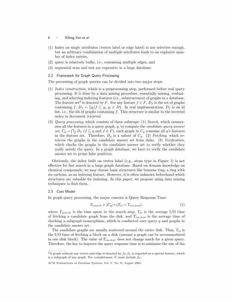
As one can see, frequent graph is a relative concept. Whether a graph is frequentor not depends on the setting of minSup. Figure 4 shows two frequent fragmentsin the sample database with minSup = 2. Suppose all the frequent fragments withminimum support minSup are indexed. Given a query graph q, if q is frequent,the graphs containing q can be retrieved directly since q is indexed. Otherwise, q



C

C

C

C

C

(a)

C

C

CC

(b)

Fig. 4. Frequent Fragments

probably has a frequent subgraph f whose support may be close to minSup. Sinceany graph with q embedded must contain q’s subgraphs, Df is a candidate answerset for query q. If minSup is low, it is not expensive to verify the graphs in Df .Therefore, it is feasible to index frequent fragments for graph query processing.

A further examination helps clarify the case where query q is not frequent ina graph database. We sort all q’s subgraphs in the support decreasing order:f1, f2, . . . , fn. There must exist a boundary between fi and fi+1 where |Dfi

|≥ minSup and |Dfi+1

| < minSup. Since all the frequent fragments with minimumsupport minSup are indexed, the graphs containing fj (1 ≤ j ≤ i) are known.Therefore, we can compute the candidate answer set Cq by

⋂

1≤j≤i Dfj, whose size

is at most |Dfi|. For many queries, |Dfi

| is close to minSup. Hence the intersec-tion of its frequent fragments,

⋂

1≤j≤i Dfj, leads to a small size of Cq. Therefore,

the cost of verifying Cq is minimal when minSup is low. This is confirmed by ourexperiments in Section 6.

The above discussion exposes our key idea in graph indexing: It is feasible toconstruct high-quality indices using only frequent fragments. Unfortunately, forlow support queries (i.e., queries whose answer set is small), the size of candidateanswer set Cq is related to the setting of minSup. If minSup is set too high, thesize of Cq may be too large. If minSup is set too low, it is too difficult to generateall frequent fragments because there may exist an exponential number of frequentfragments under low support.

Should we enforce a uniform minSup for all the fragments? Let’s examine asimple example: a completely connected graph with 10 vertices, each of which hasa distinct label. There are 45 1-edge subgraphs, 360 2-edge ones, and more than1, 814, 400 8-edge ones3. As one can see, in order to reduce the overall index size,it is appropriate for the index scheme to have low minimum support on smallfragments (for effectiveness) and high minimum support on large fragments (forcompactness). This criterion on the selection of frequent fragments for effectiveindexing is called size-increasing support constraint.

Definition 6 Frequent Pattern with Size-increasing Support. Given amonotonically nondecreasing function, ψ(l), pattern g is frequent under the size-increasing support constraint if and only if |Dg| ≥ ψ(size(g)), and ψ(l) is a size-increasing support function.

By enforcing the size-increasing support constraint, we bias the feature selectionto small fragments with low minimum support and large fragments with high min-imum support. Especially, we always set minSup to be 1 for size-0 fragment to

3For any n-vertex complete graph with different vertex labels, the number of size-k connected

subgraphs is greater than Ck+1n × (k + 1)!/2, which is the number of size-k paths (k < n).



ensure the completeness of the indexing. This method leads to two advantages: (1)the number of frequent fragments so obtained is much less than that with the low-est uniform minSup, and (2) low-support large fragments may be indexed well bytheir smaller subgraphs; thereby we do not miss useful fragments for indexing. Thefirst advantage also shortens the mining process when graphs have big structuresin common.

0 5 100

5

10

15

20

fragment size (edges)

supp

ort(

%)

Θ

θ

(a) exponential

0 5 100

5

10

15

20

fragment size (edges)

supp

ort(

%)

Θ

θ

(b) piecewise-linear

Fig. 5. Size-increasing Support Functions

Example 6. Figure 5 shows two size-increasing support functions: exponentialand piecewise-linear. We select size-1 fragments with minimum support θ and largerfragments with higher support until we exhaust fragments up to size of maxL withminimum support Θ. A typical setting of θ and Θ is 1 and 0.1N , respectively, whereN is the size of the database. We have a wide range of monotonically nondecreasingfunctions to use as ψ(l).

Using frequent fragments with the size-increasing support constraint, we have asmaller number of fragments to check their discriminative ratio. It is also interestingto examine the relationship between low supported fragments and discriminativefragments. A low supported fragment is not necessarily discriminative. For exam-ple, assume there is a low supported structure with three connected discriminativesubstructures. If this structure has the same support with one of its three substruc-tures, it is not discriminative according to Definition 5.

5. GINDEX

In this section, we present the gIndex algorithm, examine the index data structures,and discuss the incremental maintenance of indices that supports insertion anddeletion operations. We illustrate the design and implementation of gIndex infive subsections: (1) discriminative fragment selection, (2) index construction, (3)search, (4) verification, and (5) incremental maintenance.

5.1 Discriminative Fragment Selection

Applying the concepts introduced in Sections 3 and 4, gIndex first generates allfrequent fragments with a size-increasing support constraint. Meanwhile, it distillsthese fragments to identify discriminative ones. The feature selection proceeds in



a level-wise manner, i.e., Breadth-First Search (BFS). Algorithm 1 outlines thepseudo-code of feature selection.

Algorithm 1 Feature Selection

Input: Graph database D, Discriminative ratio γmin, Size-increasing supportfunction ψ(l), and Maximum fragment size maxL.

Output: Feature set F .

1: let F = {f∅}, Df∅= D, and l = 0;

2: while l ≤ maxL do

3: for each fragment x, whose size is l do

4: if x is frequent and discriminative4 then

5: F = F ∪ {x};6: l = l + 1;7: return F ;

5.2 Index Construction

Once discriminative fragments are selected, gIndex has efficient data structures tostore and retrieve them. It translates fragments into sequences and holds them in aprefix tree. Each fragment is associated with an id list: the ids of graphs containingthis fragment. We present the details of index construction in this section.

5.2.1 Graph Sequentialization. Substantial portion of computation involved inindex construction and searching is related to graph isomorphism checking. Onehas to quickly retrieve a given fragment from the index. Considering that graphisomorphism testing is hard (It is suspected to be in neither P nor NP-complete,though it is obviously in NP); it is inefficient to scan the whole feature set to matchfragments one by one. An efficient solution is to translate a graph into a sequence,called canonical label. If two fragments are the same, they must share the samecanonical label.

A traditional sequentialization method is to concatenate rows or columns of theadjacency matrix of a graph into an integer sequence. However, adjacency matrixis space inefficient for sparse graphs. In our implementation, we apply a graphsequentialization method, called DFS coding [Yan and Han 2002; 2003], to storegraphs. Certainly, other canonical labeling systems can also be used in our indexframework.

Example 7. DFS coding can translate a graph into an edge sequence, which isgenerated by performing a depth first search (DFS) in a graph. The bold edgesin Figure 6(b) constitute a DFS search tree. Each vertex is subscripted by itsdiscovery order in a DFS search. The forward edge set contains all the edgesin the DFS tree while the backward edge set contains the remaining edges. Forthe graph shown in Figure 6(b), the forward edges are discovered in the order of

4|Dx| ≥ ψ(size(x)) and |⋂

i Dfϕi|/|Dx| ≥ γmin, for fϕi ⊆ x and fϕi ∈ F .



X

a

b

b

(a)

a

v 0

X

Z Y

X

a

b

b

(b)

a X

Z Y

v 1

v 2 v 3

Fig. 6. DFS Code Generation

(v0, v1), (v1, v2), (v1, v3). Now we put backward edges into the order as follows.Given a vertex v, all of its backward edges should appear after the forward edgepointing to v. For vertex v2 in Figure 6(b), its backward edge (v2, v0) should appearafter (v1, v2). Among the backward edges from the same vertex, we can enforce anorder: given vi and its two backward edges, (vi, vj), (vi, vk), if j < k, then edge(vi, vj) will appear before edge (vi, vk). So far, we complete the ordering of edges ina graph. Based on this order, a complete edge sequence for Figure 6(b) is formed:〈(v0, v1), (v1, v2), (v2, v0), (v1, v3)〉. This sequence is called a DFS code.

We represent a labeled edge by a 5-tuple, (i, j, li, l(i,j), lj), where li and lj are thelabels of vi and vj respectively and l(i,j) is the label of the edge connecting vi andvj . Thus, the above edge sequence can be written as 〈 (0, 1, X, a, X) (1, 2, X, a,Z) (2, 0, Z, b, X) (1, 3, X, b, Y ) 〉. Since each graph can have many different DFSsearch trees and each of them forms a DFS code, a lexicographic order is designedin [Yan and Han 2002; 2003] to order DFS codes: the minimum DFS code amongg’s DFS codes is chosen as its canonical label. The readers are referred to [Yan andHan 2003] for the details of the DFS coding.

In the next subsections, we will introduce how to store and search the sequen-tialized graphs (e.g. the minimum DFS codes) of discriminative fragments.

5.2.2 gIndex Tree. Using the above sequentialization method, each fragmentcan be mapped to an edge sequence (e.g., minimum DFS code). We insert the edgesequences of discriminative fragments in a prefix tree, called gIndex Tree.

level 0

...

level 2

level 1

...

discriminative fragments

intermediate node

e 1

e 2

e 3

f 1

f 2

f 3

Fig. 7. gIndex Tree



Example 8. Figure 7 shows a gIndex tree, where each node represents a se-quentialized fragment (a minimum DFS code). For example, two discriminativefragments f1 = 〈e1〉 and f3 = 〈e1 e2 e3〉 are stored in the gIndex tree (for brevity,we use ei to represent edges in the DFS codes). Although fragment f2 = 〈e1 e2〉 isnot a discriminative fragment, we have to store f2 in order to connect the nodes f1

and f3.

The gIndex tree records all size-n discriminative fragments in level n (size-0fragments are graphs with only one vertex and no edge; the root node in the treeis f∅). In this tree, code s is an ancestor of s′ if and only if s is a prefix of s′.We use black nodes to denote discriminative fragments. White nodes (redundantfragments) are intermediate nodes which connect the whole gIndex tree. All leafnodes are discriminative fragments since it is useless to store redundant fragmentsin leaf nodes. In each black node fi, an id list (Ii), the ids of graphs containingfi, is recorded. White nodes do not have any id list. Assume we want to retrievegraphs which contain both fragments fi and fj , what we need to do is to intersectIi and Ij .

gIndex tree has two advantages: First, gIndex tree records not only discriminativefragments, but also some redundant fragments. This setting makes the Aprioripruning possible (Section 5.3.1). Secondly, gIndex tree can reduce the number ofintersection operations conducted on id lists of discriminative fragments by using(approximate) maximal fragments only (Section 5.3.2). In short, the search timeTsearch will be significantly reduced by using gIndex tree.

5.2.3 Remark on gIndex Tree Size. Upon examining the size of the gIndex tree,we find that the graph id lists associated with black nodes fill the major part ofthe tree. We may derive a bound for the number of black nodes on any path fromthe root to a leaf node. In the following discussion, we do not count the root as ablack node.

Theorem 1. Given a graph database and a minimum discriminative ratio, forany path in the gIndex tree, the number of black nodes on the path is O(logγmin

N),where N is the number of graphs in the database.

Proof. Let f0, f1, . . ., and fk−1 be the discriminative fragments on a path, wherefi ⊂ fi+1, 0 ≤ i ≤ k − 2. According to the definition of discriminative fragments,|⋂

j Dfj|/|Dfi

| ≥ γmin, where 0 ≤ j < i. Hence |Df0| ≥ γmin|Df1

| ≥ . . . ≥

γk−1min |Dfk−1

|. Since |Df0| ≤ N/γmin and |Dfk−1

| ≥ 1, we must have k ≤ logγminN .

Theorem 1 delivers the upper bound on the number of black nodes on any pathfrom the root to a leaf node. Considering the size-increasing support constraint,we have

N/γkmin ≥ |Dfk−1

| ≥ ψ(l), (4)

where l is the size of fragment fk−1 (l ≥ k − 1).

Example 9. Suppose the size-increasing support function ψ(l) is a linear func-tion: l

maxL × 0.01N , where maxL = 10. This means we index discriminativefragments whose size is up to 10. If we set γmin to be 2, from Eq. 4, we know



12k ≥ k−1

1000 . It implies the maximum value of k, i.e., the number of black nodes onany path in the gIndex tree, is less than 8.

Are there lots of graph ids recorded in the gIndex tree? For the number of idsrecorded on any path from the root to a leaf node, the following bound is obtained:

k−1∑

i=0

|Dfi| ≤ (

1

γmin+

1

γ2min

. . . +1

γkmin

)N,

where f0, f1, . . . , fk−1 are discriminative fragments on the path. If γmin ≥ 2,∑k−1

i=0 |Dfi| ≤ N . Otherwise, we have more ids to record. In this case, it is space

inefficient to record Dfi. An alternative solution is to store the differential id list,

i.e., △Dfi=

⋂

x Dfx− Dfi

, where fx ∈ F and fx ⊂ fi. Such a solution generalizesa similar idea presented by Zaki and Gouda [2003] and handles multiple rather thanone id list. The implementation of differential id list will not be examined furthersince it is beyond the scope of this study.

5.2.4 gIndex Tree Implementation. The gIndex tree is implemented using a hashtable to help locating fragments and retrieving their id lists quickly; both blacknodes and white nodes are included in the hash table. This is in lieu of a directimplementation of the tree structure. Nonetheless, the gIndex tree concept is crucialin determining the redundant (white) nodes which, as included in the index, willfacilitate the pruning of the search space.

With graph sequentialization, we can map any graph to an integer by hashing itscanonical label. We use c(g) to represent the label of a graph g, where c(g) couldbe the minimum DFS code of g or defined by other labeling systems.

Definition 7 Graphic Hash Code. Given a hash function h, a canonical la-beling function c, and a graph g, h(c(g)) is called graphic hash code.

We treat the graphic hash code as the hash value of a graph. Since two iso-morphic graphs g and g′ have the same canonical label, then h(c(g)) = h(c(g′)).Graphic hash code can help quickly locating fragments in the gIndex tree. In ourimplementation, the gIndex tree resides in the main memory, the inverted id-listsreside on disk and are cached in memory upon request.

5.3 Search

Given a query q, gIndex enumerates all its fragments up to a maximum size andlocates them in the index. Then it intersects the id lists associated with thesefragments. Algorithm 2 outlines the pseudo-code of the search step. An alternativeis to enumerate features in the gIndex tree first and then check whether the querycontains these features or not.

5.3.1 Apriori Pruning. The pseudo-code in Algorithm 2 must be optimized. Itis inefficient to generate every fragment in the query graph first and then checkwhether it belongs to the index. Imagine how many fragments a size-10 completegraph may have. We shall apply the Apriori rule: if a fragment is not in the gIndextree, we need not check its super-graphs any more. That is why we record someredundant fragments in the gIndex tree. Otherwise, if a fragment is not in the



Algorithm 2 Search

Input: Graph database D, Feature set F , Query q, and Maximum fragment sizemaxL.

Output: Candidate answer set Cq.

1: let Cq = D;2: for each fragment x ⊆ q and size(x) ≤ maxL do

3: if x ∈ F then

4: Cq = Cq ∩ Dx;5: return Cq;

feature set, one cannot conclude that none of its super-graphs will be in the featureset.

A hash table H is used to facilitate the Apriori pruning. As explained in Section5.2.4, it contains all the graphic hash codes of the nodes shown in the gIndex treeincluding intermediate nodes. Whenever we find a fragment in the query whosehash code does not appear in H, we need not check its super-graphs any more.

5.3.2 Maximal Discriminative Fragments. Operation Cq = Cq ∩ Dx is doneby intersecting the id lists of Cq and Dx. We now consider how to reduce thenumber of intersection operations. Intuitively, if query q has two fragments, fx ⊂fy, then Cq

⋂

Dfx

⋂

Dfy= Cq

⋂

Dfy. Thus, it is not necessary to intersect Cq

with Dfx. Let F (q) be the set of discriminative fragments (or indexing features)

contained in query q, i.e., F (q) = {fx|fx ⊆ q ∧ fx ∈ F}. Let Fm(q) be theset of fragments in F (q) that are not contained by other fragments in F (q), i.e.,Fm(q) = {fx|fx ∈ F (q), ∄fy, s.t., fx ⊂ fy ∧ fy ∈ F (q)}. The fragments in Fm(q)are called maximal discriminative fragments. In order to calculate Cq, we onlyneed to perform intersection operations on the id lists of maximal discriminativefragments.

5.3.3 Inner Support. The previous support definition only counts the frequencyof a fragment in a graph dataset. Actually, one fragment may appear several timeseven in one graph.

Definition 8 Inner Support. Given a graph g, the inner support of subgraphx is the number of embeddings of x in g, denoted by inner support(x, g).

Lemma 1. If g is a subgraph of G and fragment x ⊂ g, then inner support(x, g) ≤inner support(x,G).

Proof. Let ρg be an embedding of g in G. For any embedding of x in g, ρx, ρg ◦ρx

is an embedding of x in G. Furthermore, given two different embeddings of x in g,ρx and ρ′x, ρg ◦ ρx and ρg ◦ ρ′x are not the same. Therefore, inner support(x, g) ≤inner support(x,G).

GraphGrep [Shasha et al. 2002] uses the above lemma to improve the filteringpower. In order to put the inner support to use, we have to store the inner supportof discriminative fragments together with their graph id lists, which means thespace cost is doubled. The pruning power of Lemma 1 is related to the size of



queries. If a query graph is large, it is pretty efficient using inner support.

5.4 Verification

After getting the candidate answer set Cq, we have to verify whether the graphs inCq really contain the query graph. The simplest approach is to perform a subgraphisomorphism test on each graph one by one. GraphGrep [Shasha et al. 2002] pro-posed an alternative approach. It records all the embeddings of paths in a graphdatabase. Rather than doing real subgraph isomorphism testing, it performs joinoperations on these embeddings to figure out the possible isomorphism mappingbetween the query graph and the graphs in Cq. Considering there are lots of pathsin the index and each path may have tens of embeddings, we find that in somecases it does not perform well. Thus, we only implement the simplest approach inour study.

5.5 Insert/Delete Maintenance

In this section, we present our index maintenance algorithm to handle insert/deleteoperations. For each insert or delete operation, we simply update the id lists ofinvolved fragments as shown in Algorithm 3. The index maintained in this wayis still of high quality if the statistics of the original database and the updateddatabase are similar. Here, the statistics mean frequent graphs and their supportsin a graph database. If they do not change, then the discriminative fragments willnot change at all. Thus, we only need to update the id lists of those fragments inthe index, just as Algorithm 3 does. Fortunately, frequent patterns are relativelystable to database updates. A small number of insert/delete operations will notchange their distribution too much. This property becomes one key advantage ofusing frequent fragments as indexing features.

Algorithm 3 Insert/Delete

Input: Graph database D, Feature set F , Inserted (Deleted) graph g and its id gid,and Maximum fragment size maxL.

Output: Updated graph indices.

1: for each fragment x ⊆ g and size(x) ≤ maxL do

2: if x ∈ F then

3: Insert:insert gid into the id list of x;

4: Delete:delete gid from the id list of x;

5: return;

The incremental updating strategy leads to another interesting result: a singledatabase scan algorithm for index construction. Rather than mining discriminativefragments from the whole graph database, one can actually first sample a smallportion of the original database randomly, load it into the main memory, minediscriminative fragments from this small amount of data and then build the index



(with Algorithm 3) by scanning the remaining database once. This strategy cansignificantly reduce the index construction time, especially when the database islarge. Notice that the improvement comes from the efficient mining of the sampledatabase.

The index constructed by the above sampling method may have a different gIndextree structure from the one constructed from scratch. First, in the sample databasea frequent fragment may be incorrectly labeled as infrequent and be missed from theindex. Secondly, the discriminative ratio of a frequent fragment may be less thanits real value and hence be pruned occasionally. Nevertheless, the misses of somefeatures will not affect the performance seriously due to the overlappings of featuresin gIndex. The strength of our index model does not rely on a single fragment, buton an ensemble of fragments. We need not care the composition of the index toomuch as long as it achieves competitive performance. Our empirical study showsthat the quality of index based on a small sample does not deteriorate at all incomparison with the index built from scratch. In the following discussion we givean analytical study on the error bound of frequency and discriminative ratio of afragment x given a sample database. Toivonen [1996] presents the frequency errorbound of itemsets, which can also be applied to graphs.

Theorem 2. Given a fragment x and a random sample D̂ of size n, if

n ≥1

2ǫ2ln(

2

δ), (5)

the probability that |frequency(x, D̂) − frequency(x)| > ǫ is at most δ, wherefrequency (x, D̂) is the frequency of x in D̂.

Proof. [Toivonen 1996].If we want to find the complete set of frequent fragments above the minimum

support threshold, we may set a lower support in order to avoid misses with a highprobability. A variation of the above theorem was developed for this purpose.

Theorem 3. Given a fragment x, a random sample D̂ of size n, and a probabilityparameter δ, the probability that x is a miss is at most δ when

low frequency ≤ min frequency −

√

1

2nln(

1

δ), (6)

where low frequency is the lowered minimum frequency threshold and min frequencyis the requested minimum frequency threshold.

Proof. [Toivonen 1996].Theorem 3 shows that we may set a lower minimum support to solve the pattern

loss problem. However, it becomes a problem of less interest since the supportthreshold is set flexibly and empirically in our solution. We do not witness greatperformance fall for a slightly different minimum support setting. Next, we estimatethe error bound of discriminative ratio γ. Let γ̂ be the random variable thatexpresses the discriminative ratio of an arbitrary sample D̂.

Theorem 4. Given a fragment x, a set of features fϕ1, fϕ2

, . . . , fϕm, fϕi

⊆ x,



1 ≤ i ≤ m, and a random sample D̂ of size n, if

n ≥(2 + ǫ)3

pǫ2ln(

4

δ), (7)

the probability that |γ − γ̂| > ǫγ is at most δ, where p is the frequency of x and γ isits discriminative ratio with respect to fϕ1

, fϕ2, . . ., and fϕm

.

Proof. Let X be the total number of graphs in D̂ containing x. X has the binomialdistribution B(n, p), E[X] = pn. The Chernoff bounds [Alon and Spencer 1992]shows

Pr[(X − pn) > a] < e−a2/2pn+a3/2(pn)2 , (8)

Pr[(X − pn) < −a] < e−a2/2pn, (9)

where a > 0.Substituting a with ǫ′E[X] = ǫ′pn, we find

Pr[(X − pn) > ǫ′pn] < e−ǫ′2pn/2+ǫ′3pn/2 = e(ǫ′3−ǫ′2)pn/2,

P r[(X − pn) < −ǫ′pn] < e−ǫ′2pn/2 = e−ǫ′2pn/2.

Hence,

Pr[|X − pn| > ǫ′pn] < 2e(ǫ′3−ǫ′2)pn/2.

We set δ′ = 2e(ǫ′3−ǫ′2)pn/2. If

n ≥2

p(ǫ′2 − ǫ′3)ln(

2

δ′),

the probability that |X − E[X]| > ǫ′E[X] is at most δ′.Let Y be the total number of graphs in D̂, each of which has fragments fϕ1

, fϕ2, . . .,

and fϕm. Applying the Chernoff bounds again, we note that if

n ≥2

q(ǫ′2 − ǫ′3)ln(

2

δ′),

the probability that |Y − E[Y ]| > ǫ′E[Y ] is at most δ′, where q is the probabilitythat a graph contains fϕ1

, fϕ2, . . ., and fϕm

. Since fragments fϕ1, fϕ2

, . . . , fϕmare

subgraphs of x, q ≥ p. Therefore, if n ≥ 2p(ǫ′2−ǫ′3) ln( 2

δ′ ), with probability 1 − 2δ′,

both X and Y have a frequency error less than ǫ′. We have

γ − γ̂ =E[Y ]

E[X]−

Y

X

E[Y ]

E[X]−

E[Y ](1 + ǫ′)

E[X](1 − ǫ′)< γ − γ̂ <

E[Y ]

E[X]−

E[Y ](1 − ǫ′)

E[X](1 + ǫ′)

|γ − γ̂|/γ <2ǫ′

1 − ǫ′(10)

Set ǫ = 2ǫ′

1−ǫ′ and δ = 2δ′. Thus, if

n ≥(2 + ǫ)3

pǫ2ln(

4

δ), (11)



the probability that the relative error of discriminative ratio is greater than ǫ is atmost δ.

ǫ δ p n

0.2 0.05 0.1 12,000

0.2 0.05 0.05 24,000

0.1 0.01 0.1 56,000

0.1 0.01 0.05 120,000

Table I. Sufficient Sample Size Given ǫ, δ, and p

Table I shows the sufficient sample size given some typical settings of parameters.For example, we observed that the performance achieved with γmin = 2.0 is notvery different from the one with γmin = 2.4 in the chemical database we tested (seethe experiment results on the sensitivity of discriminative ratio). It implies thatthe system will still work well under a high error ratio, e.g., ǫ = 10% ∼ 20%, anda small sample.

Because of the sampling error, some valid fragments may not meet the minimumsupport constraint or pass feature selection as stated above. However, since thesetting of the size-increasing support function and the minimum discriminative ratioitself is empirical in our approach, such misses will not cause a problem. When thepatterns have very low supports, we have to scan the database to discover thesepatterns, which may require a multi-pass algorithm.

Algorithm 4 Sampling based Index Construction

Input: Graph database D and Maximum fragment size maxL.Output: Graph index I.

1: extract a sample D′ from D;2: select a feature set F from D′ (Algorithm 1);3: build an index I on D′ using the features in F ;4: for each graph g ∈ D − D′ do

5: insert g into the index I (Algorithm 3);6: return I;

Once an index is constructed using a sample, the incremental maintenance algo-rithm (Algorithm 3) will process the remaining graphs. Algorithm 4 depicts thesample-based index construction procedure. Because the mining time spent on thesample is limited, the time complexity of the sampling-based index construction isO(cN), where c is the maximum cost of updating the index for one graph and N isthe number of graphs in the database. Observe that c is usually a large constant.Thus, the sampling approach can build the index within time cost linear to thedatabase size. This result is confirmed by our experiments.



The quality of an index may degrade over time after lots of insertions and dele-tions. A measure is required to monitor the indexed features which may be out-of-

date after updates. The effectiveness of gIndex can be measured by|⋂

f Df |

|Dx|over

some set of randomly selected query graphs, where f ∈ F and f ⊆ x. This is theratio of the candidate answer set size over the actual answer set size. We monitorthe ratio based on sampled queries and check whether its average value changes overtime. A sizable increase of the value implies that the index has deteriorated, prob-ably because some discriminative fragments are missing from the indexing features.In this case, we have to consider recomputing the index from scratch.

6. EXPERIMENTAL RESULT

In this section, we report our experiments that validate the effectiveness and effi-ciency of the gIndex algorithm. The performance of gIndex is compared with that ofGraphGrep, a path-based approach [Shasha et al. 2002]. Our experiments demon-strate that gIndex achieves smaller indices and is able to outperform GraphGrepin various query loads. The effectiveness of the index returned by the incrementalmaintenance algorithm is also confirmed by our study: it performs as well as theindex computed from scratch provided the data distribution does not change much.

We use two kinds of datasets in our experiments: one real dataset and a seriesof synthetic datasets (we ignore the edge labels). Most of our experiments wereconducted on the real dataset since it is the source of real demands.

(1) The real dataset we tested is that of an AIDS antiviral screen dataset contain-ing chemical compounds. This dataset is available publicly on the website ofDevelopmental Therapeutics Program. As of March 2002, the dataset contains43,905 classified chemical molecules.

(2) The synthetic data generator was provided by Kuramochi and Karypis [Ku-ramochi and Karypis 2001]. The generator allows a user to specify the numberof graphs (D), their average size (T ), the number of seed graphs (S), the averagesize of seed graphs (I), and the number of distinct labels (L).

All our experiments are performed on a 1.5GHZ, 1GB-memory, Intel PC runningRedHat 8.0. Both GraphGrep and gIndex are compiled with gcc/g++.

6.1 AIDS Antiviral Screen Dataset

The experiments described in this section use the antiviral screen dataset. Weset the following parameters in GraphGrep and gIndex for index construction. InGraphGrep, the maximum length of indexing paths is 10: GraphGrep enumeratesall possible paths with length up to 10 and indexes them. Another parameter inGraphGrep, the fingerprint set size [Shasha et al. 2002], is set as large as possible(10k). The fingerprint set consists of the hash values of indexing features. In ourexperiments, we do not use the technique of fingerprint since it has similar effect onGraphGrep and gIndex: the smaller the fingerprint set, the smaller the index sizeand the worse the performance. In gIndex, the maximum fragment size maxL isalso 10; the minimum discriminative ratio γmin is 2.0; and the maximum supportΘ is 0.1N . The size-increasing support function ψ(l) is 1 if l < 4; in all other

cases, ψ(l) is√

lmaxLΘ. This means that all the fragments with size less than 4 are



indexed. It should be noted that the performance is not sensitive to the selectionof ψ(l). There are other size-increasing support functions which can be applied,e.g., l

maxLΘ, ( lmaxL )2Θ, and so on. We choose to have the same maximum size of

features in GraphGrep and gIndex so that a fair comparison between them can bedone.

We first test the index size of GraphGrep and gIndex. As mentioned before,GraphGrep indexes paths while gIndex uses discriminative frequent fragments. Thetest dataset, denoted by ΓN , consists of N graphs that are randomly selected fromthe antiviral screen database. Figure 8 depicts the number of features used in thesetwo algorithms with the test dataset size varied from 1, 000 to 16, 000. The curvesclearly show that the index size of gIndex is at least 10 times smaller than that ofGraphGrep. They also illustrate two salient properties of gIndex: its index size issmall and stable. When the database size increases, the index size of gIndex does notchange much. The stability of the index is due to the fact that frequent fragmentsand discriminative frequent fragments do not change much if the data have similardistribution. In contrast, the index size of GraphGrep may increase significantlybecause GraphGrep has to index all possible paths existing in a database (up to 10edges in our experiments).

103

104

105

106

0 2 4 6 8 10 12 14 16

Num

ber

of f

eatu

res

Database size (x1k)

GraphGrepgIndex

Fig. 8. Index Size

Having verified the index size of GraphGrep and gIndex, we now check theirperformance. In Section 2, we build a query cost model. The cost of a given queryis characterized by the number of candidate graphs we have to verify, i.e., the size ofcandidate answer set Cq. We average the cost in the following way: AV G(|Cq|) =∑

q∈Q |Cq|

|Q| . The smaller the cost, the better the performance. AV G(|Dq|) is the

lower bound of AV G(|Cq|). An algorithm achieving this lower bound actuallymatches the queries in the graph dataset precisely. We use the answer set ratio,AV G(|Cq|)/AV G(|Dq|), to measure the indexing strength. A ratio closer to 1 meansbetter performance.

We select Γ10,000 as the performance test dataset. Six query sets are tested, eachof which has 1, 000 queries: we randomly draw 1, 000 graphs from the antiviral



0

2

4

6

8

10

12

14

5 10 15 20 25

Ans

wer

set

rat

io (

|Cq|

/ |D

q|)

Query size

GraphGrepgIndex

Fig. 9. Low Support Queries

0

2

4

6

8

10

12

5 10 15 20 25

Ans

wer

set

rat

io (

|Cq|

/ |D

q|)

Query size

GraphGrepgIndex

Fig. 10. High Support Queries

screen dataset and then extract a connected size-m subgraph from each graphrandomly. These 1, 000 subgraphs are taken as a query set, denoted by Qm. Wegenerate Q4, Q8, Q12, Q16, Q20, and Q24. Each query set is then divided into twogroups: low support group if its support is less than 50 and high support group if itssupport is between 50 and 500. We make such elaborate partitions to demonstratethat gIndex can handle all kinds of queries very well, no matter whether they arefrequent or not and no matter whether they are large or not.

Figures 9 and 10 present the performance of GraphGrep and gIndex on lowsupport queries and high support queries, respectively. As shown in the figures,gIndex outperforms GraphGrep nearly in every query set, except the low supportqueries in query set Q4. GraphGrep works better on Q4 because queries in Q4 aremore likely path-structured and the exhausted enumeration of paths in GraphGrepfavors these queries. Another reason is that the setting of ψ(l) in gIndex has aminimum support jump on size-4 fragments (from 1 to 632).

Figure 11 shows the performance according to the query answer set size (query



1

10

102

103

104

1 10 100 1000 10000

Can

dida

te a

nsw

er s

et s

ize

(|Cq|

)

Query answer set size (|Dq|)

GraphGrepgIndex

Actual Match

Fig. 11. Performance on the Chemical Data

support), i.e., |Dq|. X axis shows the actual answer set size while Y axis shows theaverage size of the candidate answer set, |Cq|, returned by these two algorithms. Wealso plot the size of query answer set: |Dq|, which is the highest performance thatan algorithm can achieve. The closer |Cq| to |Dq|, the better the performance. Theperformance gap between gIndex and GraphGrep shrinks when the query supportincreases. The underlying reason is that higher support queries usually have simplerand smaller structures, where GraphGrep works well. When |Dq| is close to 10, 000,|Cq| will approach |Dq| since 10, 000 is its upper bound in this test. Overall, gIndexoutperforms GraphGrep by 3 to 10 times when the answer set size is below 1, 000.

Since gIndex uses frequent fragments, at the first sight, one might suspect thatgIndex may not process low support queries well. However, according to the aboveexperiments, gIndex actually performs very well on queries which have low supportsor even no match in the database. This phenomena might be a bit counter-intuitive.We find that the size-increasing support constraint and the intersection power ofstructure-based features in gIndex are the two key factors for this robust result.

150

200

250

300

350

1 1.5 2 2.5 3 3.5 4 1

10

Can

dida

te a

nsw

er s

et s

ize

(|Cq|

)

Num

ber

of f

eatu

res(

x103 )

Minimum discriminative ratio

Average of |Cq|Number of features

Fig. 12. Sensitivity of Discriminative Ratio



Next, we check the sensitivity of minimum discriminative ratio γmin. The per-formance and the index size with different γmin are depicted in Figure 12. In thisexperiment, query set Q12 is processed on dataset Γ10,000. It shows that the queryresponse time gradually improves when γmin decreases. Simultaneously, the indexsize increases. In practice, we have to make a trade-off between the performanceand the space cost.

0.001

0.01

0.1

1

10

5 10 15 20 25

Run

time(

in s

econ

ds)

Query size

gIndex: Search CostgIndex: Total CostSequential Search

Fig. 13. gIndex Runtime

Figure 13 shows the candidate search cost (Tsearch) and the total cost (overallquery response time) per query in a database with 10,000 chemical compounds.The figure also depicts the cost of brute-force search by scanning the databasesequentially. This experiment is done on various query sets, from Q4 to Q24. Itverifies that sequential subgraph isomorphism testing takes more time than can-didate filtering, suggesting that an effective index should reduce the number ofcandidate graphs as much as possible. Figure 13 also indicates the query responsetime is closer to Tsearch when query graphs are bigger. This is reasonable sincefewer graphs will become candidates for big query graphs.

The scalability of gIndex is presented in Figure 14. We vary the database sizefrom 2, 000 to 10, 000 and construct the index from scratch for each database. Werepeat the experiments for various minimum discriminative ratio thresholds. Asshown in the figure, the index construction time is proportional to the database size.The linear increasing trend is pretty predicable. For example, when the minimumdiscriminative ratio is set at 2.0, we find that the feature set mined by gIndexfor each database has around 3, 000 discriminative fragments. This number doesnot fluctuate a lot across different databases in this experiment, which may explainwhy the index construction time increases linearly. Since the size-increasing supportfunction ψ(l) follows the database size, ψ(l) ∝ Θ ∝ N , the frequent fragment setwill be relatively stable if the databases have similar distribution.

Figure 14 also shows that the index construction time does not change too muchfor a given database when the minimum discriminative ratio is above 2.0. Wefind that the construction time consists of two parts, frequent graph mining anddiscriminative feature selection. Given a database and a size-increasing support



100

200

300

400

500

600

700

800

900

1000

2000 4000 6000 8000 10000

Inde

x co

nstr

uctio

n tim

e (i

n se

cond

s)

Database size

discriminative ratio 1.0discriminative ratio 2.0discriminative ratio 4.0

Fig. 14. Scalability: Index Construction Time

function, the cost of frequent graph mining remains constant. When the ratio isbelow 2.0, the number of discriminative features does not vary much (see Figure12). Thus, the overall computation time has little deviation.

20

30

40

50

60

70

80

2000 4000 6000 8000 10000

Can

dida

te a

nsw

er s

et s

ize

(|Cq|

)

Database Size

From scratchIncremental

Fig. 15. Incremental Maintenance

The stability of frequent fragments leads to the effectiveness of our incrementalmaintenance algorithm. Assume that we have two databases D and D′ = D +∑

i D+i , where D+

i ’s are the updates over the original database D. As long as thegraphs in D and D+

i are from the same reservoir, we need not build a separateindex for D′. Instead, the feature set of D can be reused for the whole datasetD′. This remark is confirmed by the following experiment. We first take Γ2,000

as the initial dataset D, and add another 2, 000 graphs into it and update theindex using Algorithm 3. We repeat such addition and update four times until thedataset has 10, 000 graphs in total. The performance of the index obtained fromincremental maintenance is compared with the index computed from scratch. Weselect the query set Q16 to test. Figure 15 shows the comparison between these



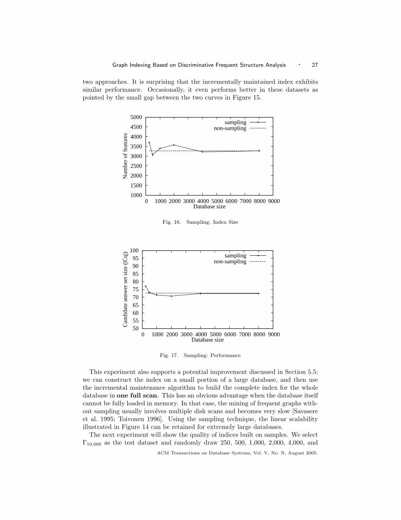
two approaches. It is surprising that the incrementally maintained index exhibitssimilar performance. Occasionally, it even performs better in these datasets aspointed by the small gap between the two curves in Figure 15.

1000

1500

2000

2500

3000

3500

4000

4500

5000

0 1000 2000 3000 4000 5000 6000 7000 8000 9000

Num

ber

of f

eatu

res

Database size

samplingnon-sampling

Fig. 16. Sampling: Index Size

50 55 60 65 70 75 80 85 90 95

100

0 1000 2000 3000 4000 5000 6000 7000 8000 9000

Can

dida

te a

nsw

er s

et s

ize

(|Cq|

)

Database size

samplingnon-sampling

Fig. 17. Sampling: Performance

This experiment also supports a potential improvement discussed in Section 5.5:we can construct the index on a small portion of a large database, and then usethe incremental maintenance algorithm to build the complete index for the wholedatabase in one full scan. This has an obvious advantage when the database itselfcannot be fully loaded in memory. In that case, the mining of frequent graphs with-out sampling usually involves multiple disk scans and becomes very slow [Savasereet al. 1995; Toivonen 1996]. Using the sampling technique, the linear scalabilityillustrated in Figure 14 can be retained for extremely large databases.

The next experiment will show the quality of indices built on samples. We selectΓ10,000 as the test dataset and randomly draw 250, 500, 1,000, 2,000, 4,000, and



8,000 graphs from Γ10,000 to form samples with different size. Totally six indicesare built on these samples and are updated by the remaining graphs in the dataset.Figures 16 and 17 depict the index size and the performance (average candidateanswer set size) of our sampling-based approach. The query set tested is Q16. Forcomparison, we also plot the corresponding curves for the index built from Γ10,000

(the dotted lines in the figures). It demonstrates the index built from small samples(e.g., 500 graphs) can achieve the same performance with the index built from thewhole dataset (10, 000 graphs). This result proves the effectiveness of our samplingmethod and the scalability of gIndex in large scale graph databases. Although theconvergence on the number of features happens only for large sampling fractions asshown in Figure 16, the performance does not fluctuate dramatically with differentsample sizes.

6.2 Synthetic Dataset

In this section, we present the performance comparison on synthetic datasets. Thesynthetic graph dataset is generated as follows: first, a set of S seed fragments isgenerated randomly, whose size is determined by a Poisson distribution with meanI. The size of each graph is a Poisson random variable with mean T . Seed fragmentsare then randomly selected and inserted into a graph one by one until the graphreaches its size. More details about the synthetic data generator are available in[Kuramochi and Karypis 2001]. A typical dataset may have the following setting:it has 10,000 graphs and uses 1,000 seed fragments with 50 distinct labels. Onaverage, each graph has 20 edges and each seed fragment has 10 edges. This datasetis denoted by D10kI10T20S1kL50.

1

10

100

1 10 100

Can

dida

te a

nsw

er s

et s

ize

(|Cq|

)

Query answer set size (|Dq|)

GraphGrepgIndex

Actual Match

Fig. 18. Performance on a Synthetic Dataset

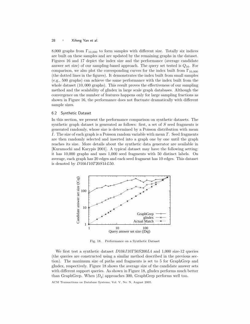
We first test a synthetic dataset D10kI10T50S200L4 and 1,000 size-12 queries(the queries are constructed using a similar method described in the previous sec-tion). The maximum size of paths and fragments is set to 5 for GraphGrep andgIndex, respectively. Figure 18 shows the average size of the candidate answer setswith different support queries. As shown in Figure 18, gIndex performs much betterthan GraphGrep. When |Dq| approaches 300, GraphGrep performs well too.



103

102

3 4 5 6 7 8 9 10 11

Can

dida

te a

nsw

er s

et s

ize

(|Cq|

)

Number of labels

GraphGrepgIndex

Fig. 19. Various Number of Labels

In some situations, GraphGrep and gIndex can achieve similar performance.When the size of query graphs is very large, the pruning based on the types ofnode and edge labels could be good enough. In this case, whether using paths orusing structures as indexing features is not important any more. When the numberof distinct labels (L) is large, the synthetic dataset is much different from the AIDSantiviral screen dataset. Although local structural similarity appears in differentsynthetic graphs, there is little similarity existing among each graph. This char-acteristic results in a simpler index structure. For example, if every vertex in onegraph has a unique label, we only need to index vertex labels. This is similar tothe inverted index technique (word - document id list) used in document retrieval.In order to verify this conclusion, we vary the number of labels from 4 to 10 in thedataset D10kI10T50S200 and test the performance of both algorithms. Figure 19shows that they are actually very close to each other when L is greater than 6.

103

102

101

20 30 40 50 60 70 80 90 100

Can

dida

te a

nsw

er s

et s

ize

(|Cq|

)

Average graph size (in edges)

GraphGrepgIndex

Fig. 20. Various Graph Size

Figure 20 depicts the performance comparison on the dataset D10kI10S200L4



with various graph sizes. In this experiment, we test 1,000 12-edge query graphs. Itshows that gIndex can still outperform GraphGrep when the graph size increases.We also tested other synthetic datasets with different parameters. Similar resultsare also observed in these experiments.

gIndex and GraphGrep have limitations on dense graph databases that have asmall number of labels. In this kind of database, the number of paths and frequentfragments increases dramatically. It is very hard to enumerate all of them. Imaginea graph becomes more and more dense, it is likely to contain any kind of querystructure, which will make candidate pruning ineffective. Fortunately, these graphsare not of practical importance. Real graphs such as chemical compounds, proteinnetworks, and image models are usually very sparse and only have a limited numberof cycles.

7. DISCUSSION

In this section, we discuss the related work and the issues for further exploration.

7.1 Related Work

The problem of graph query processing has been addressed in various fields sinceit is a critical problem for many applications. In content-based image retrieval, Pe-trakis and Faloutsos [1997] represent each graph as a vector of features and indexgraphs in high dimensional space using R-trees. Shokoufandeh et al. [1999] repre-sent and index graphs by a signature computed from the eigenvalues of adjacencymatrix. Instead of casting a graph to a vector form, Berretti et al. [2001] proposea metric indexing scheme which organizes graphs hierarchically according to theirmutual distances. The SUBDUE system developed by Holder et al. [1994] uses min-imum description length to discover substructures that compress the database andrepresent structural concepts in the data. SUBDUE is a structural pattern miningsoftware, not systematically optimized for graph query processing. In 3D proteinstructure search, algorithms using hierarchical alignments on secondary structureelements [Madej et al. 1995], or geometric hashing [Wolfson and Rigoutsos 1997],have already been developed. There are other literatures related to graph retrievalin these fields which we cannot enumerate here. In short, these systems are de-signed for other graph retrieval tasks, such as exact or similar whole graph retrieval[Petrakis and Faloutsos 1997; Shokoufandeh et al. 1999; Beretti et al. 2001] and 3Dgeometric graph retrieval [Madej et al. 1995; Wolfson and Rigoutsos 1997]. Theyare either inapplicable or inefficient to the problem studied in this paper.

In semistructured/XML databases, query languages built on path expressionsbecome popular. Efficient indexing techniques for path expression are initiallyshown in DataGuide [Goldman and Widom 1997] and 1-index [Milo and Suciu1999]. A(k)-index [Kaushik et al. 2002] further proposes k-bisimilarity to exploitlocal similarity existing in semistructured databases. APEX [Chung et al. 2002]and D(k)-index [Chen et al. 2003] consider the adaptivity of index structure to fitthe query load. Index Fabric [Cooper et al. 2001] represents every path in a tree asa string and stores it in a Patricia trie. For more complicated graph queries, Shashaet al. [Shasha et al. 2002] extend the path-based technique to do full scale graphretrieval, which is also used in Daylight system [James et al. 2003]. Srinivasa et al.[Srinivasa and Kumar 2003] build the index based on multiple vector spaces with



different abstract levels of graphs. However, no algorithm is considered to indexgraphs using frequent structures, which is the emphasis of this study.

Washio and Motoda [2003] have a general introduction on the recent progressof graph-based data mining. In frequent graph mining, Inokuchi et al. [2000], Ku-ramochi and Karypis [2001], and Vanetik et al. [2002] propose Apriori-based algo-rithms to discover frequent subgraphs. Yan and Han [2002; 2003] and Borgelt andBerthold [2002] apply the pattern-growth approach to directly generate frequentsubgraphs. In this paper, we adopt a pattern-growth approach [Yan and Han 2002]as the underlying graph mining engine because of its efficiency. Certainly, any kindof frequent graph mining algorithm can be used in the implementation becausethe mining engine itself will not influence our graph indexing results and queryperformance.

In comparison with previous methods for indexing graphs, our approach suggestsa new direction. Most of the previous indexing methods treat data in one dimensionor a combination of dimensions uniformly, i.e., either index all of them or none ofthem. For structural data, it is difficult to determine which dimension to select.gIndex performs selective indexing based on the analysis of data characteristics.Since only some of the index entries will be selected and built, gIndex substantiallyreduces the total size of indices and alleviates the combinatorial explosion problemin multi-dimensional indexing.

7.2 A New Perspective on the Applications of Frequent Pattern Mining

Frequent pattern mining was originally proposed for knowledge discovery and as-sociation rule mining [Agrawal and Srikant 1994]. Research on frequent patternmining has been focused on how to develop efficient algorithms for mining frequentpatterns in large databases and how to identify interesting frequent patterns usingdifferent measures. However, since frequent pattern information represents inher-ent data characteristics, its application should not be confined to data mining only.Through our study, we broaden the scope of the application of frequent patternmining and bring the usage of frequent patterns to a new perspective: frequentpatterns are used as basic building blocks for indexing and database management.We show that due to the complexity of structured data like graphs, it is impossibleto index all the substructures, and discriminative frequent pattern analysis will leadus to the development of compact but effective index structures. In this case, weare not interested in whether an individual discriminative frequent pattern exposessome knowledge. Instead, all of discriminative frequent patterns work together toachieve impressive performance.

7.3 Extensions to Single Graph Indexing

Although gIndex is about indexing multiple graphs, it can naturally extend totackling the single graph indexing problem: Given a single large graph and a querygraph, the task is to discover all the subregions (or subgraphs) where the querygraph is embedded. Many applications have the demand of searching interestingunits in a massive graph such as biological network, social network and circuit.Several issues have to be addressed in order to make the extension successful. First,we need an algorithm to mine frequent structures in a single graph. Fortunately, thesolution is already available [Kuramochi and Karypis 2004]. Second, a positioning



scheme should be devised to assign the positions for each structure in the graph,which can facilitate the intersection operation (similar to

⋂

f Df in gIndex). Notethat an efficient intersection operation is very critical to the performance since bothdiscriminative ratio computation and query processing rely on this operation. Afterwe obtain all discriminative features through feature selection, we may apply thetechniques developed in this paper to construct the indices and process the queriesin a single graph.

7.4 Issues for Further Exploration

The indexing strategy proposed in this paper can be categorized into a new theme:discriminative frequent pattern-based (DFP) indexing. It is radically differentfrom traditional indexing methods. It best fits those applications where single-dimensional indexing is not selective, multi-dimensional indexing is explosive, queryis bulky, and search within complex objects is costly. We believe in such applica-tions, the previous indexing methods encounter real challenges. There are lots ofunanswered questions calling for further exploration. We name a few as follows.

First, it is important to broaden the application domains and explore the bound-ary of our approach. Obviously, we can apply DFP in sequence or tree databases.Nevertheless, there are many applications where the traditional indexing approachmay still have its edge. For example, for gene network indexing, since genes arehighly selective and user queries in many cases are also not bulky (e.g., contain-ing only several genes), it is likely that the traditional inverted indexing approachwill be a better choice. Another question is if the analyzed graphs have nearly nocommon subgraphs or always have big structures in common, how well does gIndexperform? The answer is positive as to indexing performance. However, it mayencounter difficulties in index construction since gIndex intends to enumerate allfrequent patterns in big common structures. The recent work on closed frequentgraph mining [Yan and Han 2003] provides a solution by skipping the search spaceefficiently.

Second, we have assumed all the features are of homogeneous type, such asdiscriminative subgraphs, or discriminative subsequences. However, features canbe of heterogeneous type in some cases. For example, in graph mining, one mayconsider not only subgraphs but also subsequences or subsets as features. In certainapplications, this may reduce the number of features to be indexed and furtherenhance the efficiency of search.

Third, we considered only exact matching queries in graphs. However, in practice,there are many applications where the approximate matching is desirable. Forexample, in DNA sequence analysis, approximate matching on DNA subsequencesis expected since mutation, insertion, and deletion are normal in genome sequences.Similar cases apply to image, video, chemical compound, and network flow analysis.It is an interesting research problem to see how the DFP indexing approach shouldbe further developed for such applications.

8. CONCLUSIONS

Indexing complex and structured objects to facilitate the processing of nontrivialqueries is an important task in database applications. In this study, we analyze whythe traditional indexing approach may encounter challenges in these applications



and propose a new indexing methodology: discriminative frequent pattern-basedindexing. This new indexing methodology is based on frequent pattern mining anddiscriminative feature selection. Our study on graph indexing shows that DFP leadsto compact index, better query processing efficiency, and easy maintenance due tostable indexing structures. We believe our study may attract further explorationof new methods for indexing complex objects by integration of sophisticated datamining and data analysis techniques.

9. ACKNOWLEDGMENTS

The work was done in IBM T.J. Watson Research Center and University of Illinoisat Urbana-Champaign. The work of the first and third authors is supported inpart by the U.S. National Science Foundation NSF IIS-02-09199, the Universityof Illinois, and an IBM Faculty Award. Any opinions, findings, and conclusionsor recommendations expressed in this paper are those of the authors and do notnecessarily reflect the views of the funding agencies. We would like to thank RosalbaGiugno and Dennis Shasha for providing GraphGrep; and Michihiro Kuramochi andGeorge Karypis for providing the synthetic graph data generator. The authors aregrateful to anonymous reviewers for their constructive and helpful comments onthe initial versions of the paper.

REFERENCES

Agrawal, R. and Srikant, R. 1994. Fast algorithms for mining association rules. In Proc. 1994

Int. Conf. on Very Large Data Bases (VLDB’94). Santiago, Chile, 487–499.

Alon, N. and Spencer, J. 1992. The Probabilistic Method. John Wiley Inc., New York, NY.

Beretti, S., Bimbo, A., and Vicario, E. 2001. Efficient matching and indexing of graph mod-els in content-based retrieval. IEEE Transactions on Pattern Analysis and Machine Intelli-

gence 23, 1089–1105.

Borgelt, C. and Berthold, M. 2002. Mining molecular fragments: Finding relevant substruc-

tures of molecules. In Proc. 2002 Int. Conf. on Data Mining (ICDM’02). Maebashi, Japan,211–218.

Chen, Q., Lim, A., and Ong, K. 2003. D(k)-index: An adaptive structural summary for graph-structured data. In Proc. 2003 ACM-SIGMOD Int. Conf. on Management of Data (SIG-MOD’03). San Diego, CA, 134 – 144.

Chung, C., Min, J., and Shim, K. 2002. Apex: An adaptive path index for xml data. In Proc.2002 ACM-SIGMOD Int. Conf. on Management of Data (SIGMOD’02). Madison, WI, 121 –

132.

Cook, S. The complexity of theorem-proving procedures. In Proc. 3rd ACM Symp. on Theory

of Computing (STOC’71). Shaker Heights, OH.

Cooper, B., Sample, N., Franklin, M., Hjaltason, G., and Shadmon, M. 2001. A fast indexfor semistructured data. In Proc. 2001 Int. Conf. on Very Large Data Bases (VLDB’01).

Roma, Italy, 341–350.

Goldman, R. and Widom, J. 1997. Dataguides: Enabling query formulation and optimization

in semistructured databases. In Proc. 1997 Int. Conf. on Very Large Data Bases (VLDB’97).Athens, Greece, 436–445.

Holder, L., Cook, D., and Djoko, S. 1994. Substructure discovery in the subdue system. InProc. AAAI’94 Workshop on Knowledge Discovery in Databases (KDD’94). Seattle, WA, 169

– 180.

Inokuchi, A., Washio, T., and Motoda, H. 2000. An apriori-based algorithm for mining frequentsubstructures from graph data. In Proc. 2000 European Symp. Principle of Data Mining and

Knowledge Discovery (PKDD’00). Lyon, France, 13–23.



James, C., Weininger, D., and Delany, J. 2003. Daylight theory manual daylight version 4.82.

Daylight Chemical Information Systems, Inc.

Kaushik, R., Shenoy, P., Bohannon, P., and Gudes, E. 2002. Exploiting local similarity

for efficient indexing of paths in graph structured data. In Proc. 2000 Int. Conf. on DataEngineering (ICDE’02). San Jose, CA, 129–140.

Kuramochi, M. and Karypis, G. 2001. Frequent subgraph discovery. In Proc. 2001 Int. Conf.Data Mining (ICDM’01). San Jose, CA, 313–320.

Kuramochi, M. and Karypis, G. 2004. Finding frequent patterns in a large sparse graph. In

Proc. 2004 SIAM Int. Conf. on Data Mining (SDM’04). Orlando, FL.

Madej, T., Gibrat, J., and Bryant, S. 1995. Threading a database of protein cores. Proteins 3-

2, 289–306.

Milo, T. and Suciu, D. 1999. Index structures for path expressions. Lecture Notes in Computer

Science 1540, 277–295.

Petrakis, E. and Faloutsos, C. 1997. Similarity searching in medical image databases. Knowl-

edge and Data Engineering 9, 3, 435–447.

Savasere, A., Omiecinski, E., and Navathe, S. 1995. An efficient algorithm for mining associ-

ation rules in large databases. In Proc. 1995 Int. Conf. Very Large Data Bases (VLDB’95).Zurich, Switzerland, 432–443.

Shasha, D., Wang, J., and Giugno, R. 2002. Algorithmics and applications of tree and graph

searching. In Proc. 21th ACM Symp. on Principles of Database Systems (PODS’02). Madison,WI, 39–52.

Shokoufandeh, A., Dickinson, S., Siddiqi, K., and Zucker, S. 1999. Indexing using a spectralencoding of topological structure. In Proc. IEEE Int. Conf. on Computer Vision and Pattern

Recognition (CVPR’99). Fort Collins, CO, 2491–2497.

Srinivasa, S. and Kumar, S. 2003. A platform based on the multi-dimensional data modelfor analysis of bio-molecular structures. In Proc. 2003 Int. Conf. on Very Large Data Bases

(VLDB’03). Berlin, Germany, 975–986.

Toivonen, H. 1996. Sampling large databases for association rules. In Proc. 1996 Int. Conf. on

Very Large Data Bases (VLDB’96). Bombay, India, 134–145.

Vanetik, N., Gudes, E., and Shimony, S. E. 2002. Computing frequent graph patterns from

semistructured data. In Proc. 2002 Int. Conf. on Data Mining (ICDM’02). Maebashi, Japan,458–465.

Washio, T. and Motoda, H. 2003. State of the art of graph-based data mining. SIGKDDExplorations 5, 59–68.

Wolfson, H. and Rigoutsos, I. 1997. Geometric hashing: An introduction. IEEE ComputationalScience and Engineering 4, 10–21.

Yan, X. and Han, J. 2002. gSpan: Graph-based substructure pattern mining. In Proc. 2002 Int.

Conf. on Data Mining (ICDM’02). Maebashi, Japan, 721–724.

Yan, X. and Han, J. 2003. CloseGraph: Mining closed frequent graph patterns. In Proc. 2003

Int. Conf. on Knowledge Discovery and Data Mining (KDD’03). Washington, D.C., 286–295.

Zaki, M. and Gouda, K. 2003. Fast vertical mining using diffsets. In Proc. 2003 Int. Conf. on

Knowledge Discovery and Data Mining (KDD’03). Washington, DC, 326–335.


Documents

Graph Indexing Based on Discriminative Frequent Structure