Graph Attribute Embedding via Riemannian

Submersion Learning

Haifeng Zhao4 Antonio Robles-Kelly1,2,3 Jun Zhou1,2,3

Jianfeng Lu4 Jing-Yu Yang4

1 NICTA∗, Locked Bag 8001, Canberra ACT 2601, Australia

2 The Australian National University, Canberra ACT 0200, Australia

3 UNSW@ADFA, Canberra ACT 2600, Australia

4 Nanjing University of Science and Technology, Nanjing 210094, China

Abstract

In this paper, we tackle the problem of embedding a set of relational structures into a metric

space for purposes of matching and categorisation. To this end, we view the problem from a

Riemannian perspective and make use of the concepts of charts on the manifold to define the

embedding as a mixture of class-specific submersions. Formulated in this manner, the mixture

weights are recovered using a probability density estimation on the embedded graph node

coordinates. Further, we recover these class-specific submersions making use of an iterative

trust-region method so as to minimise the L2 norm between the hard limit of the graph-vertex

posterior probabilities and their estimated values. The method presented here is quite general

in nature and allows tasks such as matching, categorisation and retrieval. We show results

on graph matching, shape categorisation and digit classification on synthetic data, the MNIST

dataset and the MPEG-7 database.

Keywords: Graph embedding; Riemannian geometry; relational matching∗NICTA is funded by the Australian Government as represented by the Department of Broadband, Communications

and the Digital Economy and the Australian Research Council through the ICT Centre of Excellence program.

1

1 Introduction

The problem of embedding relational structures onto a manifold arises in parameterization of three-

dimensional data [1], multidimensional scaling (MDS)[2], graph drawing [3] and structural graph

matching [4]. In the pattern analysis community, there has recently been renewed interest in us-

ing embedding methods motivated by graph theory for representation, classification, retrieval or

visualisation.

The aim along these lines is to recover a mapping of the relational structure under study so

as to minimise a measure of distortion. An option here is to perform graph interpolation by a

hyperbolic surface which has the same pattern of geodesic, i.e. internode, distances as the graph

[5]. Collectively, these methods are sometimes referred to as manifold learning theory. In [6], a

manifold is constructed whose triangulation is the simplical complex of the graph. Other methods,

such as ISOMAP [7], focus on the recovery of a lower-dimensional embedding which is quasi-

isometric in nature. Related algorithms include locally linear embedding [8], which is a variant

of PCA that restricts the complexity of the input data using a nearest neighbor graph. Belkin

and Nigoyi [9] present a Laplacian eigenmap which constructs an adjacency weight matrix for the

data-points and projects the data onto the principal eigenvectors of the associated Laplacian matrix.

Embedding methods can also be used to transform the relational-matching problem into one of

point-pattern matching in a high-dimensional space. The problem is to find matches between pairs

of point sets when there is noise, geometric distortion and structural corruption. The problem arises

in shape analysis [10], motion analysis [11] and stereo reconstruction [12]. As a result, there is

a considerable literature on the problem, and many contrasting approaches, including search [13]

and optimisation [14] have been attempted. However, the main challenge in graph matching is how

to deal with differences in node and edge structure.

Further, the main argument levelled against the work above is that they adopt a heuristic ap-

proach to the relational matching problem by using a goal-directed graph similarity measure. To

overcome this problem, several authors have adopted a more general approach using ideas from

information and probability theory. For instance, Wong and You [15] defined an entropic graph-

distance for structural graph matching. Christmas, Kittler and Petrou [16] have shown how a re-

2

laxation labeling approach can be employed to perform matching using pairwise attributes whose

distribution is modeled by a Gaussian. Wilson and Hancock [17] have used a maximum a pos-

teriori (MAP) estimation framework to accomplish purely structural graph matching. Recently,

Caetano et al. [18] have proposed a method to estimate the compatibility functions for purposes of

learning graph matching.

One of the most elegant recent approaches to the graph matching problem has been to use graph

spectral methods [19], which exploits the information conveyed by the graph spectra, i.e. the

eigenvalues and eigenvectors of the adjacency matrix or the Combinatorial Laplacian. There have

been successful attempts to use spectral methods for both structural graph matching [20] and point

pattern matching [21, 12]. For instance, Umeyama [20] has developed a method for finding the

permutation matrix which best matches pairs of weighted graphs of the same size, by using a sin-

gular value decomposition of the adjacency matrices. Scott and Longuet-Higgins [21], on the other

hand, align point-sets by performing singular value decomposition on a point association weight

matrix. Shapiro and Brady [12] have reported a correspondence method which relies on measur-

ing the similarity of the eigenvectors of a Gaussian point-proximity matrix. Although Umeyama’s

algorithm [20] is elegant in its formulation and can deal with both weighted or unweighted graphs,

it can not be applied to graphs which contain different numbers of nodes and for weighted graphs

the method is susceptible to weight errors. One way to overcome these problems is to cast the

problem of recovering correspondences in a statistical setting using the EM algorithm [22].

Spectral methods can be viewed as embedding the nodes of a graph in a space spanned by

the eigenvectors of the adjacency matrix. In the case of Umeyama’s algorithm [20], matching is

effected by finding the transformation matrix that best aligns the embedded points. The Shapiro

and Brady [12] algorithm finds correspondences by seeking the closest embedded points. Kosinov

and Caelli [23] have improved this method by allowing for scaling in the eigenspace. Robles-

Kelly and Hancock [24] make use of the relationship between the Laplace-Beltrami operator and

the graph Laplacian so as to embed a graph onto a Riemannian manifold.

An alternative approach to inexact graph matching is that of computing a metric that reflects the

overall cost of the set of edit operations required to transform one graph into another. The idea

is to measure the similarity of graphs by counting the number of graph edit operations i.e. node,

3

edge insertions and deletions. The concept of string edit distance has been extended to graphs by

Sanfeliu and Fu [25], Eshera and Fu [26] and Shapiro and Haralick [27]. These methods pose the

problem of computing a metric for measuring the similarity between two graphs as that of finding a

common underlying topological structure through graph edit operations. This is closely related to

the problem of measuring structural affinity using the maximum common subgraph. Myers, Wilson

and Hancock [28] have shown how the method in [17] can be rendered more effective making use

of the Levenshtein string edit distance. Furthermore, Rice, Bunke and Natker [29] showed the

relationship between a particular set of cost functions and the longest common subsequence for a

pair of strings. More recently, Sebastian and Kimia [30] have used a distance metric analogous to

the string edit distance to perform object recognition from a dataset of shock graphs.

The maximum common subgraph is an important subject in graph theory and has been used

to solve relational matching problems [31, 32]. The maximum common subgraph can be used to

depict common topology and, as a result, it is a powerful tool for graph matching and object recog-

nition. Unfortunately, the maximum common subgraph is not unique and does not depend on the

index of the nodes of the graph. Moreover, the computation of the maximum common subgraph is

an NP-complete problem. As a result, conventional algorithms for computing the maximum com-

mon subgraph have an exponential computational cost. Although these algorithms are simple to

understand and code, their computational cost is high due to the fact they are usually based on max-

imal clique detection [33] or backtracking [34]. To overcome this problem, practical algorithms

for computing the maximum common subgraph often rely upon approximate constraints to over-

come the exponential complexity problem and achieve polynomial cost. For instance, Messmer

and Bunke [35] have proposed a graph-error correction algorithm that runs in polynomial time.

In this paper, we aim at presenting a method to embed the graph vertex-attributes into a space

where distances between nodes correspond the structural differences between graphs. This can be

viewed as a learning process in which the aim of computation is the recovery of a set of linear

operators, which map the node-set of a graph onto a metric space. Viewed from a Riemannian

perspective, the embedding is given by a mixture of submersions governed by a kernel density

estimation process. This leads to a formulation of the problem where the embedding space is

spanned by an operator which minimises the L2 norm between the hard limit of the graph-vertex

4

posterior probabilities and their value estimated from class-specific information. The embedding

presented here permits the use of metrics in the target space for purposes of categorisation and

relational matching tasks. Moreover, it provides a link between structural and statistical pattern

recognition techniques through differential geometry.

Thus, the formulation presented here has a number of advantages. Firstly, it permits matching

and categorisation tasks to be performed using simple point-pattern matching methods in a unified

framework by embedding graph nodes into a metric space. Secondly, we draw on the properties

of operators on Riemannian manifolds [36]. This implies that the embedding is linked directly

to the geometry of the underlying graph class. Moreover, the work presented here provides a

means to graph embedding through Riemannian geometry and optimisation on manifolds which

employ invariant subspaces of matrices [37]. Finally, the optimisation method presented here is

quite general in nature. The method is devoid of parameters and can be considered as a trust-region

method over a group of invariant matrix manifolds.

2 Riemannian Geometry

In this section, we provide the theoretical basis for our graph embedding method. Consider a set

of graphs Γ partitioned into a set of classes Ω = ω1, ω2, . . . , ω|Ω|. Here, we develop a method

to employ class-specific information to embed the graphs in Γ into a manifold using Riemannian

submersions. This can be viewed as a learning process, in which the embedding is recovered from

labeled, i.e. categorised, graphs. Thus, as input to the training step, the method takes a set of

graphs whose nodes attributes are given by a set of vectors, and delivers, at output, a model which

can be used for embedding graphs which are are not in the training set.

This section is organised as follows. We commence by providing the necessary background on

Riemannian manifolds. We then formulate the embedding as a mixture of Riemannian submersions

arising from the set of charts corresponding to a set of submanifolds for the clusters in Ω. With

this formulation at hand, we turn our attention to the recovery of the submersions themselves by

optimising a cost function based upon the L2 norm on the posterior probabilities for the graph-

vertices given the class information.

5

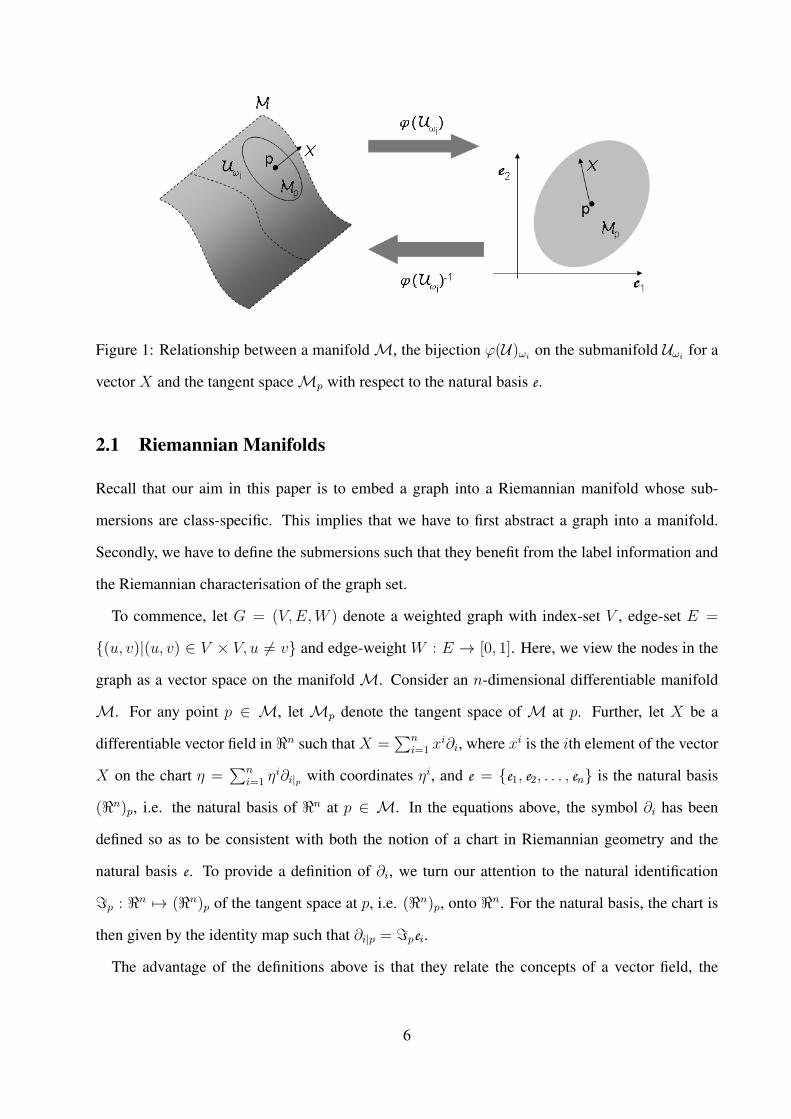
Figure 1: Relationship between a manifoldM, the bijection ϕ(U)ωion the submanifold Uωi

for a

vector X and the tangent spaceMp with respect to the natural basis e.

2.1 Riemannian Manifolds

Recall that our aim in this paper is to embed a graph into a Riemannian manifold whose sub-

mersions are class-specific. This implies that we have to first abstract a graph into a manifold.

Secondly, we have to define the submersions such that they benefit from the label information and

the Riemannian characterisation of the graph set.

To commence, let G = (V,E,W ) denote a weighted graph with index-set V , edge-set E =

(u, v)|(u, v) ∈ V × V, u 6= v and edge-weight W : E → [0, 1]. Here, we view the nodes in the

graph as a vector space on the manifold M. Consider an n-dimensional differentiable manifold

M. For any point p ∈ M, let Mp denote the tangent space of M at p. Further, let X be a

differentiable vector field in <n such that X =∑n

i=1 xi∂i, where xi is the ith element of the vector

X on the chart η =∑n

i=1 ηi∂i|p with coordinates ηi, and e = e1, e2, . . . , en is the natural basis

(<n)p, i.e. the natural basis of <n at p ∈ M. In the equations above, the symbol ∂i has been

defined so as to be consistent with both the notion of a chart in Riemannian geometry and the

natural basis e. To provide a definition of ∂i, we turn our attention to the natural identification

=p : <n 7→ (<n)p of the tangent space at p, i.e. (<n)p, onto <n. For the natural basis, the chart is

then given by the identity map such that ∂i|p = =pei.

The advantage of the definitions above is that they relate the concepts of a vector field, the

6

tangent bundle and the notion of chart so as to study graphs, i.e. objects, associated with a sub-

manifold U ∈ M through a bijection ϕ(U). Moreover, we can now see the collection of charts for

every cluster in the graph set as an atlas A ofM such that ϕ(Uωi) ϕ(Uωj

)−1 : <n 7→ <n, where

we have written Uωito imply that the submanifold Uωi

corresponds to the ith cluster ωi in the graph

set Γ. In Figure 1, we use a manifoldM in <3 to provide some intuition on the formalism above.

Note that the bijection ϕ(U)ωimaps the submanifold Uωi

onto the plane spanned by the natural

basis e, which, in this case, corresponds to <2.

In the following section we ellaborate further on how this formulation permits viewing the graph

nodes as a vector field on a manifold which can be submerged into a Riemannian space. This pro-

vides the flexibility and formalism of the tools and techniques available from the field of differential

geometry and, moreover, information geometry [38].

2.2 Embeddings, Submersions and Charts

Note that the idea of chart endows the graph abstracted into a vector spaceX with a manifold struc-

ture. This manifold structure is bestowed upon the vector space X and, therefore, the topology of

the graph G has to be used to recover the vector field in such a manner that it encodes structural

information. In our experiments, we have used vertex-neighbourhood information to recover the

attributes used by our embedding. A more principled use of neighborhoods and cliques may be

formalised through the application of branched coverings [39], which operate on vertex neigh-

bourhoods. Moreover, branched coverings generalise to arbitrary dimensions in a straightforward

manner and are structure preserving in a topological sense [40].

For now, we leave open the manner in which the graph-vertices are represented by the vector

space X . As mentioned above, we will examine this further in the Experiments section. Note that

we can use the idea of bijection between the natural basis andM and a submersion F :M 7→ Uωi

to embed the graphs in the set Γ. We can then view the F as a transformation matrix such that

Y = FX . Thus, given the coordinates in <n for all the nodes in the graph-set Γ the purpose is

to find a transformation matrix F ∈<n×d that projects the input vectors for the nodes in the graph

onto the submanifold Uωisuch that Y = FX belongs to a lower dimensional space <d(d 6 n)

7

maximising the separation between classes in Ω and the affinity within classes.

Following the chart and atlas concepts presented above, there must be a smooth transition be-

tween charts across the submanifolds Uωi. Moreover, consider the posterior probability P (G | ωi)

of a graph in Γ belonging to the cluster ωi. Ideally, if a graph belongs to a given cluster, the

posterior P (G | ωi) should be unity if and only if the graph belongs to the class ωi, i.e.

P (X | G ∈ ωi) =

1 if G ∈ ωi

0 otherwise(1)

By relaxing the hard limit above for P (X | G ∈ ωi) ∈ [0, 1], we can write the embedding for

the nodes in G as a mixture of the form

Y ∗ =

|Ω|∑i=1

P (X | G ∈ ωi)FωiX (2)

where, as before, we have written Fωito imply that the submersion corresponds to the cluster ωi.

Thus, for the atlas, the submersion is then given by the mixture

F ∗ =

|Ω|∑i=1

P (X | G ∈ ωi)Fωi(3)

In Figure 2, we illustrate the geometric meaning of our embedding approach. In the figure, we

show a manifoldM ∈ <3 akin to that in Figure 1. Here, the submersions Fωiand Fωj

correspond

to two clusters in the graph set Γ. Note that, despite these being mutually independent, the tangent

bundle Mp “overlaps” the submanifolds Uωiand Uωj

. Following the figure, we can view the

posterior probabilities αi(Y ) = P (X | G ∈ ωi) as weights that govern the contributions of the

submersions to the node embedding Y ∗. This is consistent with our premise above regarding the

smooth transition between the tangent spaces of Uωiand Uωj

. Note that the embedding thus hinges

in the computation of both, the submersions and the posteriors. For the remainder of the section, we

ellaborate on the computation of the posterior probabilities. In the following section we show how

the recovery of the submersions can be effected through an optimisation whose aim of computation

is to maximise separation between classes and affinity within clusters.

Recall that, since label information is at hand, we have at our disposal the true values, i.e. the

hard limits, of the posterior probabilities. Furthermore, the posterior probability density functions

8

Figure 2: Geometric interpretation of our embedding approach.

can be estimated from the data using Kernel Density Estimation (KDE) [41]. This suggests an

optimisation approach to the problem in which the posterior probabilities can be estimated from

the submerged graph nodes while the submersions themselves can be optimised upon. Thus, from

now on, we use the shorthand αi(Y ) to denote the posterior probabilities given by

αi(Y ) = P (X | G ∈ ωi) =KDEi[Fωi

X]∑|Ω|k=1KDEk[Fωk

X](4)

where KDEi[·] is the evaluation of the Kernel Density Estimator trained using the vectors Y =

FωiX corresponding to the nodes in those graphs G ∈ ωi.

2.2.1 Optimisation

Now, we turn our attention to the recovery of the submersion Fωi. To this end, we make use of the

hard limits of the posterior P (X | G ∈ ωi) so as to formulate a cost function which we can then

optimise accordingly. Recall that, if the graph G is in the cluster ωi, the posterior should be unity

and zero otherwise. Thus we can define the cost function as the L2 norm expressed as follows

D =

|Ω|∑i=1

∑V ∈GG∈ωi

| 1− αi(Y ) |2 +a‖Fωi‖ =

|Ω|∑i=1

∑V ∈GG∈ωi

g(Y, ξ)2 (5)

where a is a regularisation constant.

In the cost function above, the first term is zero when the posterior given by αi(Y ) is unity.

That is, the term tends to zero as the posterior is closer to its hard limit. The second term is a

regularisation one which encourages sparseness upon the submersions Fωi. As a result, the cost

9

function is minimum when the posteriors achieve their hard limit values making use of sparse

submersions.

With the cost function at hand, we now turn our attention to its extremisation. For the minimi-

sation of the target function we have used a manifold-based variant of the Levenberg Marquardt

[42] approach. The Levenberg-Marquardt Algorithm (LMA) is an iterative trust region procedure

[43] which provides a numerical solution to the problem of minimising a function over a space

of parameters. For purposes of minimising the cost function, we commence by writing the cost

function above in terms of the parameter set, which in this case corresponds to the entries of the

submersions Fωi. Let ξ = [V EC(Fω1), V EC(Fω2), . . . , V EC(Fω|Ω|)]

T be the parameter vector at

iteration t, where V EC(·) : <n×d 7→ <nd is an operator that takes a matrix as input and delivers

a vector as output. At each iteration, the new estimate of the parameter set is defined as ξ + δ,

where δ is an increment in the parameter space and ξ is the current estimate of the transformation

parameters. To determine the value of δ, let g(Y, ξ) =√| 1− αi(Y ) |2 +a‖Fωi

‖ be the posterior

probability evaluated at time t approximated using a Taylor series such that

g(Y, ξ + δ) ≈√| 1− αi(Y ) |2 +a‖Fωi

‖+ J (Y )δ (6)

where J (Y ) is the Jacobian of ∂g(Y,ξ+δ)∂ξ

.

The set of equations that need to be solved for δ is obtained by equating to zero the derivative

with respect to δ of the equation resulting from substituting Equation 6 into the cost function D.

Let the matrix J be comprised by the entries ∂g(Y,ξ+δ)∂ξ

, i.e. the element indexed k, i of the matrix

J is given by the derivative of αi(Y ) with respect to the kth element of the vector ξ for every

graph-node in the set Γ. We can write the resulting equations in compact form as follows

(JTJ)δ = JT [G∗ −G(ξ)] (7)

where G(ξ) is a vector whose elements correspond to the values g(Y, ξ) and G∗ is a vector whose

elements correspond to the extreme values of the function g(·) for every X in those graphs in Γ

such that | G∗ −G(ξ) | becomes minimal.

Recall that Levenberg [44] introduced a “damped” analogue of the equation above given by

(JTJ + βI)δ = JT [G∗ −G(ξ)] (8)

10

β is damping factor adjusted at each iteration and I is the identity matrix. In [42], the identity

matrix I above is substituted with the diagonal of the Hessian matrix JTJ thus yielding

(JTJ + βdiag[JTJ])δ = JT [G∗ −G(ξ)] (9)

where diag[·] is an operator that yields a diagonal matrix.

Note that, within the trust region, the minimiser of the cost function is the solution of the Gauss-

Newton Equation [43]. Since we have formulated the approach in terms of matrix manifolds [37],

we can employ an approximate Hessian, which is positive definite making use of the gradient of

the function such that

(JTJ + E)Xt = −∇G(ξ) (10)

where Xt is an iterate on the tangent bundle of the matrix manifold and E is an operator chosen

such that the convergence of the Newton iteration is superlinear, i.e.

limt→∞

| g(Y, ξ − δ) + 1 || g(Y, ξ) |

= 0 (11)

It can be shown that if | E |< 1, then (I− E)−1 exists and satisfies the following relation

| (I− E)−1 |> 1

1− | E |(12)

We refer the reader to [37] for the proof of the relations above.

In general, we can view∇ as a connection on the matrix manifold. As a result, Equation 10 can

be rewritten as

AXt = −ζ (13)

where A = JTJ + E and the entries of the vector ζ can be viewed as an object that connect

tangent spaces on the manifold over the vector field spanned by Xt at the current estimate of ξ,

i.e. ζξ = ∇Xtζ . This tells that, by construction, we have constrained the solution of the Newton

iteration to a retraction Rξ of Xt from the tangent bundle to the manifold at each iterate Xt such that

the vector ζ is parallel transported along Xt.

Moreover, we can view Equation 13 as an eigenvalue problem on the matrix A and aim at

recovering the iterate such that the gradient of G(ξ) is maximum. This procedure can be interpreted

as a gradient descent on the manifold. Note that, from the relations in Equations 11 and 12, we

11

can set E = ∅, i.e. a matrix whose entries are all nil, and make A = JTJ. Thus, let τ by the

eigenvector corresponding to the leading eigenvalue ς of A, following the developments above,

we can compute the current connection ζ = ςτ and set the natural basis e on the manifold so as to

coincide with the current iterate on the tangent bundle ofM. Thus, we have

ζ = −(JTJ + βdiag[JTJ]) • e (14)

The increment δ can be recovered by substituting Equation 14 into Equation 9, which yields

δ = −1

ζ• (JT [G∗ −G(ξ)]) (15)

= −1

ζ• (JT [G(ξ)])

where the last line above proceeds from the fact that the extreme values of g(·) are zero, i.e. we

aim at minimising D, and • denotes the Hadamard (entry-wise) product between the vectors 1ζ

and

JT [G∗ − G(ξ)]. Note that, in Equation 15, the computation of the increment δ is devoid of the

damping factor β in Equation 8 with a superlinear convergence rate.

It is worth mentioning that no assumptions on the extreme values of the function g(·) were made

in the derivation above until the second line of Equation 15 was reached. This is important since it

implies that the method above can be employed for other tasks requiring non-linear least squares

optimisers. Moreover, the method above can be viewed as an LMA one where the damping factor

has been absorbed into the eigenvalue formulation in Equation 13. Thus, the method combines the

benefits of a damped trust-region approach being devoid of parameters.

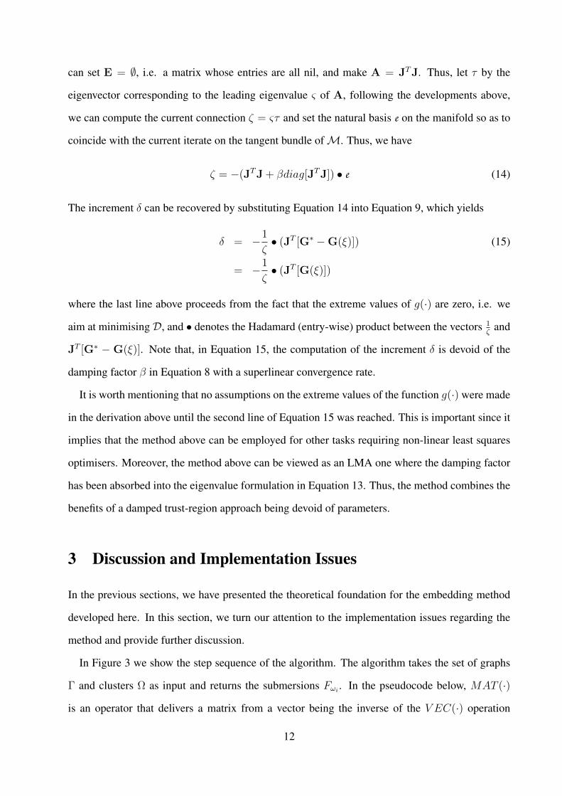
3 Discussion and Implementation Issues

In the previous sections, we have presented the theoretical foundation for the embedding method

developed here. In this section, we turn our attention to the implementation issues regarding the

method and provide further discussion.

In Figure 3 we show the step sequence of the algorithm. The algorithm takes the set of graphs

Γ and clusters Ω as input and returns the submersions Fωi. In the pseudocode below, MAT (·)

is an operator that delivers a matrix from a vector being the inverse of the V EC(·) operation

12

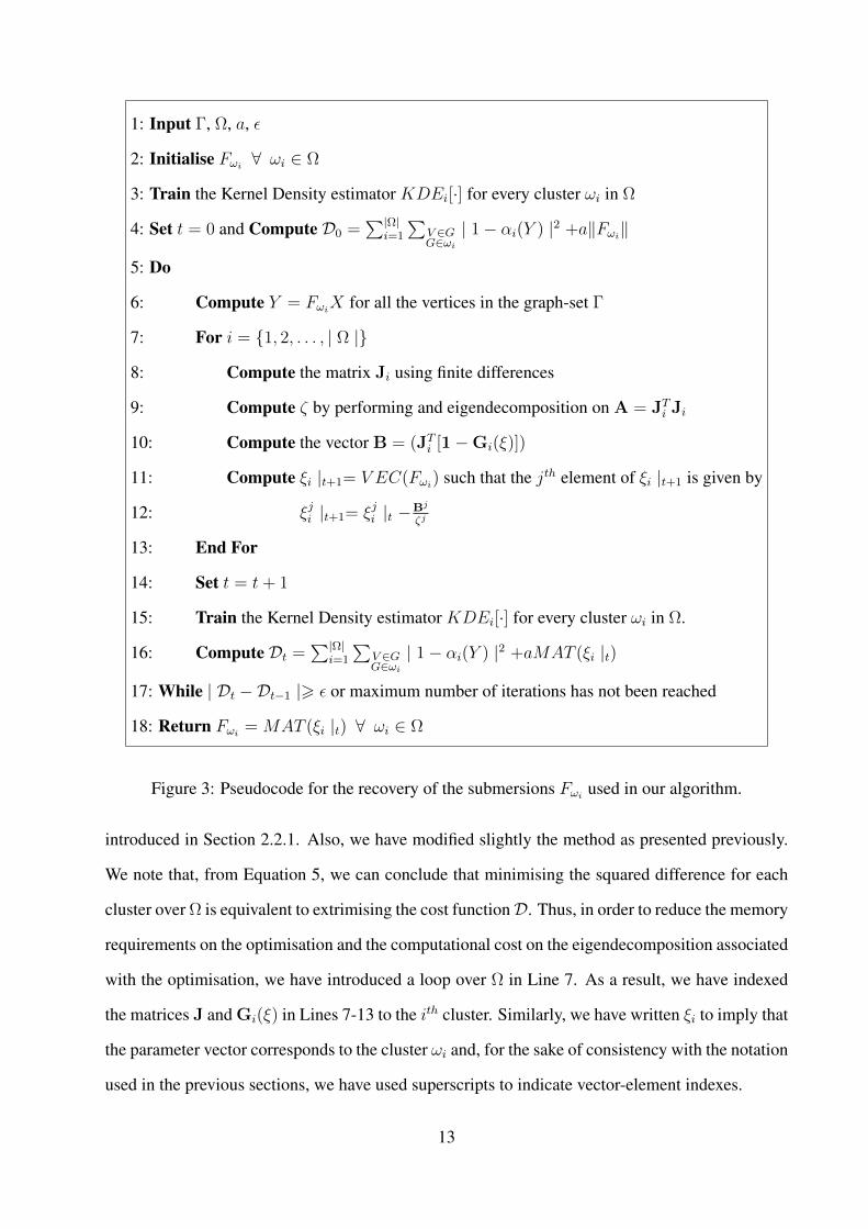
1: Input Γ, Ω, a, ε

2: Initialise Fωi∀ ωi ∈ Ω

3: Train the Kernel Density estimator KDEi[·] for every cluster ωi in Ω

4: Set t = 0 and Compute D0 =∑|Ω|

i=1

∑V ∈GG∈ωi

| 1− αi(Y ) |2 +a‖Fωi‖

5: Do

6: Compute Y = FωiX for all the vertices in the graph-set Γ

7: For i = 1, 2, . . . , | Ω |

8: Compute the matrix Ji using finite differences

9: Compute ζ by performing and eigendecomposition on A = JTi Ji

10: Compute the vector B = (JTi [1−Gi(ξ)])

11: Compute ξi |t+1= V EC(Fωi) such that the jth element of ξi |t+1 is given by

12: ξji |t+1= ξji |t −Bj

ζj

13: End For

14: Set t = t+ 1

15: Train the Kernel Density estimator KDEi[·] for every cluster ωi in Ω.

16: Compute Dt =∑|Ω|

i=1

∑V ∈GG∈ωi

| 1− αi(Y ) |2 +aMAT (ξi |t)

17: While | Dt −Dt−1 |> ε or maximum number of iterations has not been reached

18: Return Fωi= MAT (ξi |t) ∀ ωi ∈ Ω

Figure 3: Pseudocode for the recovery of the submersions Fωiused in our algorithm.

introduced in Section 2.2.1. Also, we have modified slightly the method as presented previously.

We note that, from Equation 5, we can conclude that minimising the squared difference for each

cluster over Ω is equivalent to extrimising the cost functionD. Thus, in order to reduce the memory

requirements on the optimisation and the computational cost on the eigendecomposition associated

with the optimisation, we have introduced a loop over Ω in Line 7. As a result, we have indexed

the matrices J and Gi(ξ) in Lines 7-13 to the ith cluster. Similarly, we have written ξi to imply that

the parameter vector corresponds to the cluster ωi and, for the sake of consistency with the notation

used in the previous sections, we have used superscripts to indicate vector-element indexes.

13

It is worth noting that, being a trust region method, the algorithm in Figure 3 is sensitive to

initialisation. To overcome this drawback, in the initialisation step in Line 2, we have used the set

of submersions Fωiwhich correspond to the linear subspace projection that best separates every

class from the others. One of the most popular methods for recovering these linear combinations in

supervised learning is Linear Discriminant Analysis (LDA). Here, a transformation matrix Fωi∈

<n×d is determined so as to maximise the Fisher criterion given by

H (F Tωi

) = tr((FωiSwF

Tωi

)−1(FωiSbF

Tωi

))

Sw =∑X∈GG∈ωi

(X −mi)(X −mi)T

Sb = (mi −m)(mi −m)T

=

|Ω|∑j=1

pj(mi −mj)(mi −mj)T (16)

where | Ω | is the number of classes, mj and m are the class mean and sample mean vectors,

respectively, and pi = P (ωi) is the prior probability of class ωi given by the contribution of the ith

class to the sample set X = XG∈Γ. Also, in the equations above, Sw and Sb represent the within

and between-class scatter matrices. Note that the matrix Sw can be regarded as the average class-

specific covariance, whereas Sb can be viewed as the mean distance between all different classes.

Thus, the purpose of Equation 16 is to maximise the between-class scatter while preserving within-

class dispersion in the transformed feature space. This is effected by affine projecting the inverse

intraclass covariance matrix and solving the generalised eigenvalue problem SbFTωi

= λSwFTωi

. As

the rank of Sb is | Ω | −1, the solution, for the | Ω | classes, is obtained by taking the eigenvectors

corresponding to the largest | Ω | −1 eigenvalues of S−1w Sb [45].

As presented above, the optimisation implies that the posterior αi(Y ) would be evaluated at

every iteration t. This, in turn, assumes the method trains the KDE at every iteration. This is as the

submersion Fωiis updated at every t and, hence, the model for the KDE varies accordingly. In our

implementation, we have used a Normal, i.e. Gaussian, kernel.

Note that Equation 14 employs the natural basis e so as to coincide with the iterates on the

tangent bundle of the manifold M. Since the elements of the natural basis are, by definition,

orthogonal with respect to one another [46], we can view the vector Y as a projection of the vector

14

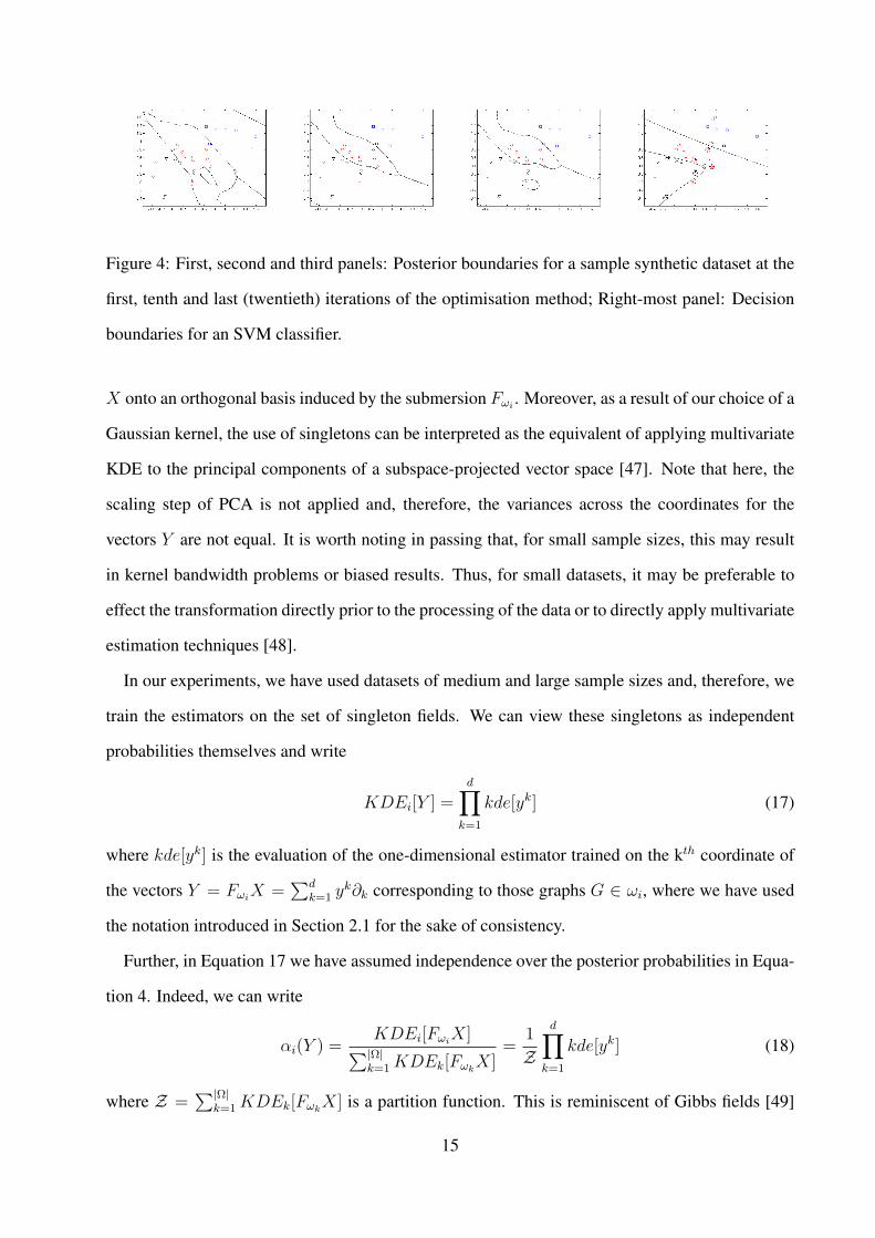
Figure 4: First, second and third panels: Posterior boundaries for a sample synthetic dataset at the

first, tenth and last (twentieth) iterations of the optimisation method; Right-most panel: Decision

boundaries for an SVM classifier.

X onto an orthogonal basis induced by the submersion Fωi. Moreover, as a result of our choice of a

Gaussian kernel, the use of singletons can be interpreted as the equivalent of applying multivariate

KDE to the principal components of a subspace-projected vector space [47]. Note that here, the

scaling step of PCA is not applied and, therefore, the variances across the coordinates for the

vectors Y are not equal. It is worth noting in passing that, for small sample sizes, this may result

in kernel bandwidth problems or biased results. Thus, for small datasets, it may be preferable to

effect the transformation directly prior to the processing of the data or to directly apply multivariate

estimation techniques [48].

In our experiments, we have used datasets of medium and large sample sizes and, therefore, we

train the estimators on the set of singleton fields. We can view these singletons as independent

probabilities themselves and write

KDEi[Y ] =d∏

k=1

kde[yk] (17)

where kde[yk] is the evaluation of the one-dimensional estimator trained on the kth coordinate of

the vectors Y = FωiX =

∑dk=1 y

k∂k corresponding to those graphs G ∈ ωi, where we have used

the notation introduced in Section 2.1 for the sake of consistency.

Further, in Equation 17 we have assumed independence over the posterior probabilities in Equa-

tion 4. Indeed, we can write

αi(Y ) =KDEi[Fωi

X]∑|Ω|k=1 KDEk[Fωk

X]=

1

Z

d∏k=1

kde[yk] (18)

where Z =∑|Ω|

k=1 KDEk[FωkX] is a partition function. This is reminiscent of Gibbs fields [49]

15

which can be modelled through Markovian processes in undirected graphs. Moreover, this formu-

lation permits the application of our method to non-attributed, but rather weighted graphs by, for

instance, using the edge-weights as the potentials of a Markov Random Field. This treatment has

been employed for purposes of segmentation [50] and more generally in [51].

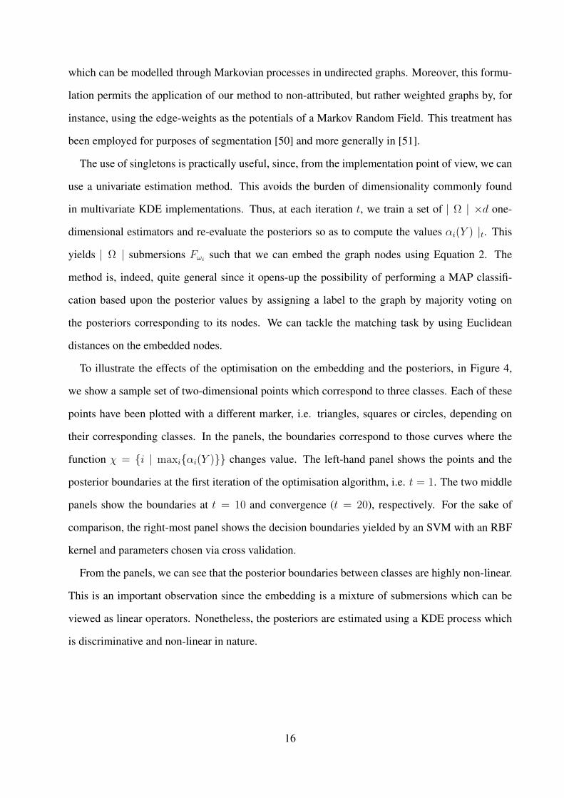
The use of singletons is practically useful, since, from the implementation point of view, we can

use a univariate estimation method. This avoids the burden of dimensionality commonly found

in multivariate KDE implementations. Thus, at each iteration t, we train a set of | Ω | ×d one-

dimensional estimators and re-evaluate the posteriors so as to compute the values αi(Y ) |t. This

yields | Ω | submersions Fωisuch that we can embed the graph nodes using Equation 2. The

method is, indeed, quite general since it opens-up the possibility of performing a MAP classifi-

cation based upon the posterior values by assigning a label to the graph by majority voting on

the posteriors corresponding to its nodes. We can tackle the matching task by using Euclidean

distances on the embedded nodes.

To illustrate the effects of the optimisation on the embedding and the posteriors, in Figure 4,

we show a sample set of two-dimensional points which correspond to three classes. Each of these

points have been plotted with a different marker, i.e. triangles, squares or circles, depending on

their corresponding classes. In the panels, the boundaries correspond to those curves where the

function χ = i | maxiαi(Y ) changes value. The left-hand panel shows the points and the

posterior boundaries at the first iteration of the optimisation algorithm, i.e. t = 1. The two middle

panels show the boundaries at t = 10 and convergence (t = 20), respectively. For the sake of

comparison, the right-most panel shows the decision boundaries yielded by an SVM with an RBF

kernel and parameters chosen via cross validation.

From the panels, we can see that the posterior boundaries between classes are highly non-linear.

This is an important observation since the embedding is a mixture of submersions which can be

viewed as linear operators. Nonetheless, the posteriors are estimated using a KDE process which

is discriminative and non-linear in nature.

16

4 Experiments

Now we turn our attention to the applicability of the embedding method to relational matching,

shape categorisation and object classification tasks. To this end, we have used three datasets. The

first of these is a synthetic one which comprises graphs of different sizes, i.e. 50, 100, 150 and 200

nodes. The second set is the MNIST handwritten digit database [52]. The third dataset is given

by the MPEG-7 CE-Shape-1 shape database, which contains 1400 binary shapes of 70 different

classes with 20 images in each category. In all our experiments we have set a = 0.01 for the cost

function in Equation 5. It is worth noting in passing that, in our experiments, the method was quite

robust to the value of a.

4.1 Synthetic Graphs

We commence by performing experiments on synthetic data. To this end, we have generated graphs

making use of randomly distributed point-sets of different sizes. These two-dimensional point-sets

comprise the nodes of our synthetically generated data. We have computed two kinds of relational

structures whose edges are given by the complete graphs and Delaunay triangulations [41] of the

point-clouds under study. For each point-set order, i.e. 50, 100, 150 and 200, we have generated

20 point-clouds. Here, for purposes of comparison, we perform graph matching and compare our

results with those yielded by the graduated assignment method of Gold and Rangarajan [14], the

discrete relaxation algorithm in [53] and the graph seriation method in [54].

For the all-connected graphs, we use vectors X whose entries are given by the normalised his-

togram of pairwise Euclidean distances between the node of reference and the rest of the nodes

in the graph. That is, given the node u, its corresponding vector X is given by the histogram of

Euclidean distances d(u, v) between the point-coordinates of u and those of v ∈ V . For the Delau-

nay triangulations, the vector X for the node u is given by the first k pairwise Euclidean distances

d(u, v), sorted in ascending rank order.

Note that the Delaunay graphs, together with other point neighbourhood graphs, such as the

k-nearest neighbour graph, Gabriel graph and the relative neighbourhood graph, is sensitive to

node deletion errors [55]. This implies that, for purposes of providing a sensitivity analysis on the

17

embedding method presented here, Delaunay graphs provide a means to evaluate the dependency

of the embedding on the structural information and its robustness to change due to noise corruption

and node deletion. Moreover, we have formulated the method in such manner that the embeddings

are effected so as to operate on the vectors X , which are used to abstract the graph-nodes into

a vector field. Hence, the effects of noise corruption or deletion on the all-connected relational

structures should be much less severe than that exhibited by the Delaunay triangulations. This is

due to the fact that the histograms used as the X vectors for the nodes of the all connected graphs

can be viewed as a discrete approximation of the pairwise distance distribution for the points in G.

This is in contrast with the Delaunay triangulations, where the vectors X have been formulated so

as to reflect the structure of the edge-set rather than the pairwise distances for the node-set.

In our sensitivity study, we examine the effects of random node-deletions and the consequences

of adding zero-mean Gaussian noise with increasing variance to the point-coordinates before the

Delaunay triangulation computation. Thus, in the case of the node deletion experiments shown

here, we have randomly deleted, in intervals of 5%, up to 50% of the graph nodes, i.e. points in

the cloud. We have done this over 10 trials for each 5% interval, which yielded 2000 graphs for

each of the four graph-sizes above, i.e. 8000 point-clouds in total. In the case of the Delaunay

triangulations, these are computed after node deletion is effected.

To evaluate the effects of noise corruption, we have added zero-mean Gaussian noise of in-

creasing variance to the 2D-coordinates of the point-sets used in our experiments. As for our

node-deletion sensitivity study, we have computed the Delaunay triangulations after the Gaussian

noise has been added. Here, we have increased the variance in steps of 0.05 up to 0.5 over 10 trials,

i.e. 10 × 20 = 200 graphs for each of the point-sets under study, which as for the node-deleted

graphs, yields 8000 graphs in total.

For the computation of the vector fields, we have used 10 histogram bins (all connected graphs)

and k = 5 (Delaunay triangulations). For both graph types, i.e. all-connected and Delaunay tri-

angulations, we have computed 20 submersions using the graphs recovered from the point-clouds

devoid of deletions. We use these deletions so as to embed the remaining graphs into a space in

which matching can be effected using a nearest-neighbour approach based upon Euclidean dis-

tances between the model and the data graphs, i.e. the one from which the submersion was com-

18

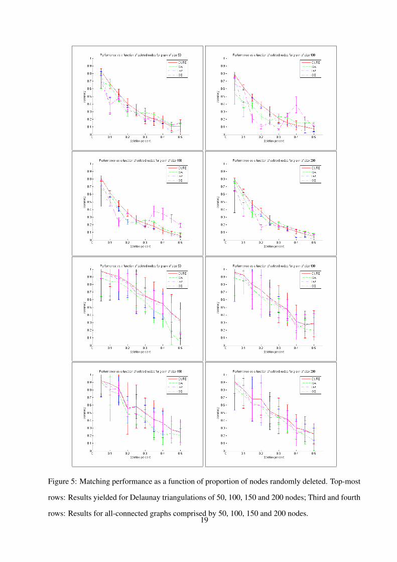
Figure 5: Matching performance as a function of proportion of nodes randomly deleted. Top-most

rows: Results yielded for Delaunay triangulations of 50, 100, 150 and 200 nodes; Third and fourth

rows: Results for all-connected graphs comprised by 50, 100, 150 and 200 nodes.19

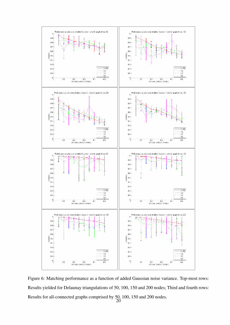
Figure 6: Matching performance as a function of added Gaussian noise variance. Top-most rows:

Results yielded for Delaunay triangulations of 50, 100, 150 and 200 nodes; Third and fourth rows:

Results for all-connected graphs comprised by 50, 100, 150 and 200 nodes.20

puted and the relational structure we aim at matching against the model. Thus, a node v in the

model graph GM is a match to a node u in the data graph GD such that argminu∈GDd(u, v) =

argminu∈GD(Yu−Yv)2, where the vector Yu corresponds to the submerged, i.e. embedded, vec-

torX corresponding to the node u. This is, u and v match if and only if they are nearest neighbours

in the submersion corresponding to the model graph GM .

In Figure 5 we show the plots for the accuracy, in percentage of correctly matched nodes, as

a function of percentage of deleted nodes for the four graph sizes in our dataset. In the panels,

the error-bars account for the standard deviation across each of the ten graphs for every node-

deletion proportion from 0.05 to 0.5, with each line-style denoting a different approach, i.e. our

method, the graduated assignment (GA) algorithm, the discrete relaxation (DR) approach and the

graph seriation (GS) method. In the figure, the two top-most rows correspond to the Delaunay

triangulations, whereas the third and fourth rows show the accuracy plots for the all-connected

graphs.

In Figure 6, we repeat the sequence above for the noise-corrupted graphs. Note that, from the

plots in Figures 5 and 6, the method provides a margin of improvement over the alternatives for

low and moderate amounts of corruption when used to match both, the Delaunay triangulations and

the all-connected graphs. Our embedding method is comparable to the alternatives even for large

amounts of noise corruption or proportion of nodes deleted, being more stable than the alterna-

tives. This is particularly evident as compared to the graph seriation (GA) method, which delivers

better results in average with an increasing standard deviation. This illustrates the ability of the

embedding to capture structural information. Moreover, when all-connected graphs are used, the

sensitivity to noise corruption or node deletion is low. This is due to the the fact that the X vectors

have been constructed making use of a pairwise histogram as an alternative to the rank ordering

of the pairwise distances for those nodes comprising cliques in the Delaunay triangulations. This

sensitivity differences between the Delaunay triangulations and the all-connected graphs are in

accordance with the developments in [55].

21

4.2 Digit Classification

Now we illustrate the ability of our method to embed graph attributes extracted from a real-world

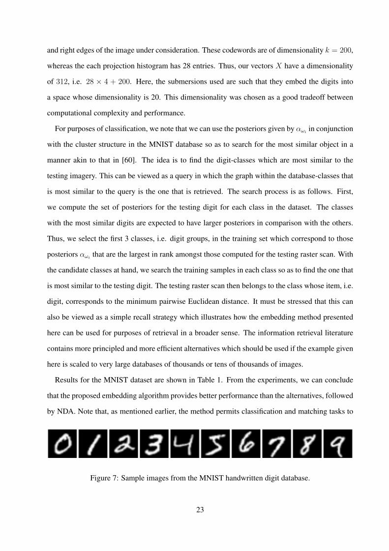
dataset. To this end, we show results on digit classification making use of the MNIST dataset.

The MNIST database which contains a training set of 60, 000 gray-scale images of handwritten

digits from 0 to 9, and a testing set of 10, 000 images. Sample handwritten digits in the dataset

are shown in Figure 7. The image sizes are 28 × 28. We have chosen the dataset due to its size

and its widespread use in the literature. We stress in passing that the aim in this section is not to

develop an OCR algorithm but rather to provide a quantitative study on a large, real-world dataset

comparing our embedding approach with other subspace projection methods. Note that there are

a wide variety of OCR techniques that have been applied to the dataset. As these are out of the

scope of this paper, for a detailed list we refer the reader to the MNIST website 1.

As mentioned earlier, one of the advantages of the strategy adopted here is that it provides

a means to connect structural techniques with statistical pattern recognition methods through a

general method for matching, categorisation and classification. As a result, we focus on the com-

parison of our method to other embedding techniques. These are Linear Discriminant Analysis

(LDA) [45], the Maximum Margin Criterion (MMC) [56] and Nonparametric Discriminant Anal-

ysis (NDA) [45]. Note that these are subspace projection methods that employ linear transfor-

mations so as to recover the optimal projection direction for the classification task at hand. Here,

classification using the alternatives is based on a feature space with dimensionality reduced to 9, i.e.

the number of classes minus 1. To compare the methods on an equal basis, for all the alternatives

we have used a 1-nearest-neighbour classifier [57].

For our digit classification experiments we have used a codebook-based approach for recovering

the vectors X . To recover the feature vectors, we commence by binarising the digits using the

thresholding method of Otsu [58]. With the binary imagery at hand, we have recovered frequency

pairwise-distance histograms between pixels on the digit contours. From these histograms, we

have computed a codebook via k-means clustering. This codebook is used to compute codewords

which are then concatenated to the projection histograms [59] with respect to the upper, lower, left

1http://yann.lecun.com/exdb/mnist/

22

and right edges of the image under consideration. These codewords are of dimensionality k = 200,

whereas the each projection histogram has 28 entries. Thus, our vectors X have a dimensionality

of 312, i.e. 28 × 4 + 200. Here, the submersions used are such that they embed the digits into

a space whose dimensionality is 20. This dimensionality was chosen as a good tradeoff between

computational complexity and performance.

For purposes of classification, we note that we can use the posteriors given by αωiin conjunction

with the cluster structure in the MNIST database so as to search for the most similar object in a

manner akin to that in [60]. The idea is to find the digit-classes which are most similar to the

testing imagery. This can be viewed as a query in which the graph within the database-classes that

is most similar to the query is the one that is retrieved. The search process is as follows. First,

we compute the set of posteriors for the testing digit for each class in the dataset. The classes

with the most similar digits are expected to have larger posteriors in comparison with the others.

Thus, we select the first 3 classes, i.e. digit groups, in the training set which correspond to those

posteriors αωithat are the largest in rank amongst those computed for the testing raster scan. With

the candidate classes at hand, we search the training samples in each class so as to find the one that

is most similar to the testing digit. The testing raster scan then belongs to the class whose item, i.e.

digit, corresponds to the minimum pairwise Euclidean distance. It must be stressed that this can

also be viewed as a simple recall strategy which illustrates how the embedding method presented

here can be used for purposes of retrieval in a broader sense. The information retrieval literature

contains more principled and more efficient alternatives which should be used if the example given

here is scaled to very large databases of thousands or tens of thousands of images.

Results for the MNIST dataset are shown in Table 1. From the experiments, we can conclude

that the proposed embedding algorithm provides better performance than the alternatives, followed

by NDA. Note that, as mentioned earlier, the method permits classification and matching tasks to

Figure 7: Sample images from the MNIST handwritten digit database.

23

Classification Method Our Method LDA MMC NDA

Classification Rate 96.12% 87.52% 86.92% 88.39%

Table 1: Percentage of correctly classified digits for our method as compared with the alternatives.

be effected in a metric space allowing for a wide variety of features to be used as vectors X .

This is important since, in our experiments, we have not preprocessed the data or performed any

stabilisation operation on the digits. These tasks can be easily introduced into our method without

any loss of generality. Moreover, despite the fact that our testing strategy does not use intensive

search as that for the alternatives, we still obtain a performance improvement for more than 8% as

compared with non-linear LDA [45] and maximum margin criterion [56].

Note that, despite the X vectors are of dimensionality 312, our approach is quite robust to

changes in dimensionality and, due to the use of singletons for the KDE estimators, is not overly

affected by the curse of dimensionality. Moreover, our descent method is based upon an eigenvalue

estimation step for which computational methods exist so as to deal with very large dimensions,

i.e. thousands of dimensions. This is consistent with our experiments, where we have not noticed

serious drops in performance as a result of employing larger dimensionalities in our frequency

histograms.

4.3 Shape Categorisation and Matching

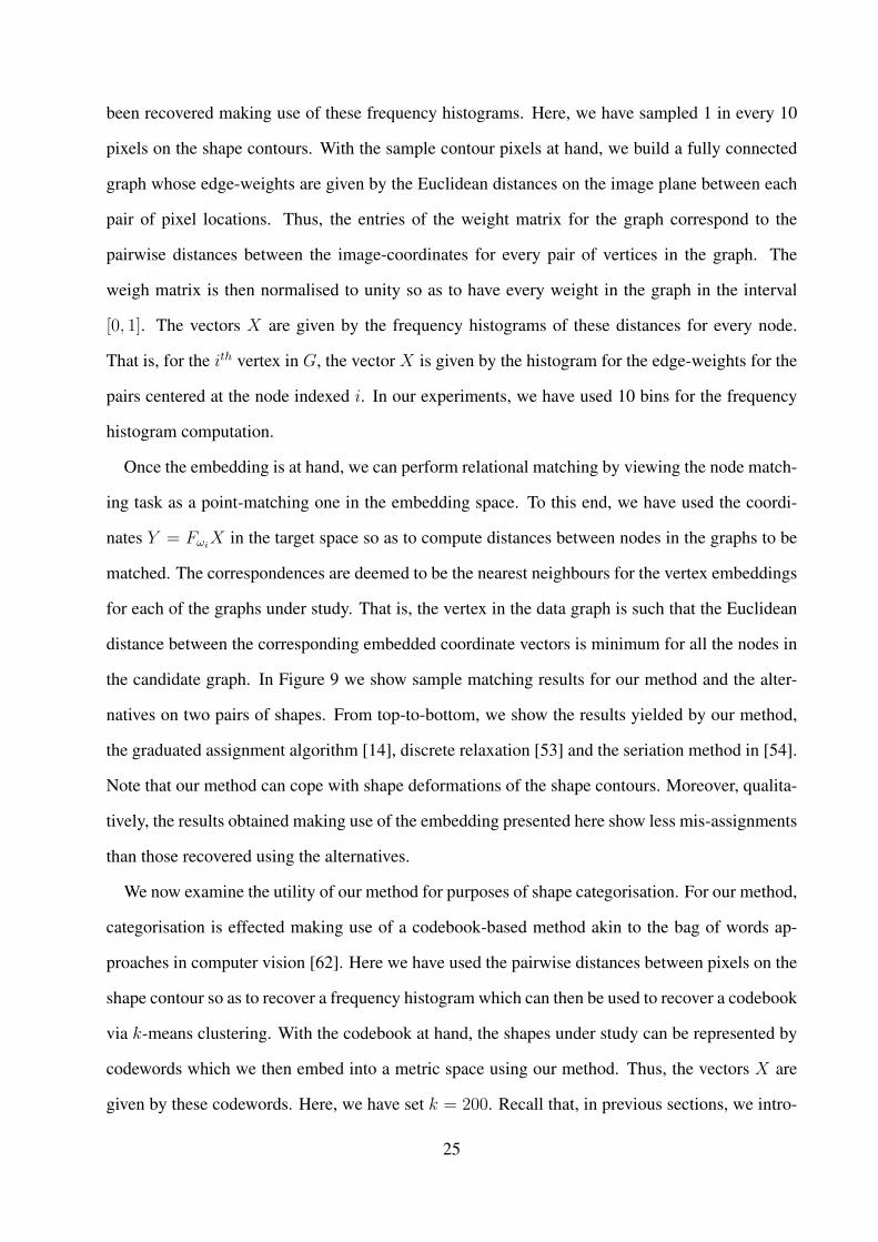
Now, we turn our attention to shape categorisation. To this end, we use the MPEG-7 CE-1 Part B

database [61]. The database contains 1400 binary shapes organised in 70 classes, each comprised

of 20 images. In Figure 8, we show some example shapes for the MPEG-7 dataset. For the MPEG-

7 CE-Shape-1 shape database, we employ the histogram of pairwise distances in the embedding

space to define the vectors X . We do this in an analogue manner to that used in the previous

sections for matching all-connected synthetic graphs and MNIST digits. We construct a graph

for each shape, where the pixels on the contour are the nodes and the X vectors are given by the

pairwise-distance frequency histograms between adjacent vertices, i.e. points on the contour.

The submersions for our method, i.e. one for each of the 70 shape categories in the dataset, have

24

been recovered making use of these frequency histograms. Here, we have sampled 1 in every 10

pixels on the shape contours. With the sample contour pixels at hand, we build a fully connected

graph whose edge-weights are given by the Euclidean distances on the image plane between each

pair of pixel locations. Thus, the entries of the weight matrix for the graph correspond to the

pairwise distances between the image-coordinates for every pair of vertices in the graph. The

weigh matrix is then normalised to unity so as to have every weight in the graph in the interval

[0, 1]. The vectors X are given by the frequency histograms of these distances for every node.

That is, for the ith vertex in G, the vector X is given by the histogram for the edge-weights for the

pairs centered at the node indexed i. In our experiments, we have used 10 bins for the frequency

histogram computation.

Once the embedding is at hand, we can perform relational matching by viewing the node match-

ing task as a point-matching one in the embedding space. To this end, we have used the coordi-

nates Y = FωiX in the target space so as to compute distances between nodes in the graphs to be

matched. The correspondences are deemed to be the nearest neighbours for the vertex embeddings

for each of the graphs under study. That is, the vertex in the data graph is such that the Euclidean

distance between the corresponding embedded coordinate vectors is minimum for all the nodes in

the candidate graph. In Figure 9 we show sample matching results for our method and the alter-

natives on two pairs of shapes. From top-to-bottom, we show the results yielded by our method,

the graduated assignment algorithm [14], discrete relaxation [53] and the seriation method in [54].

Note that our method can cope with shape deformations of the shape contours. Moreover, qualita-

tively, the results obtained making use of the embedding presented here show less mis-assignments

than those recovered using the alternatives.

We now examine the utility of our method for purposes of shape categorisation. For our method,

categorisation is effected making use of a codebook-based method akin to the bag of words ap-

proaches in computer vision [62]. Here we have used the pairwise distances between pixels on the

shape contour so as to recover a frequency histogram which can then be used to recover a codebook

via k-means clustering. With the codebook at hand, the shapes under study can be represented by

codewords which we then embed into a metric space using our method. Thus, the vectors X are

given by these codewords. Here, we have set k = 200. Recall that, in previous sections, we intro-

25

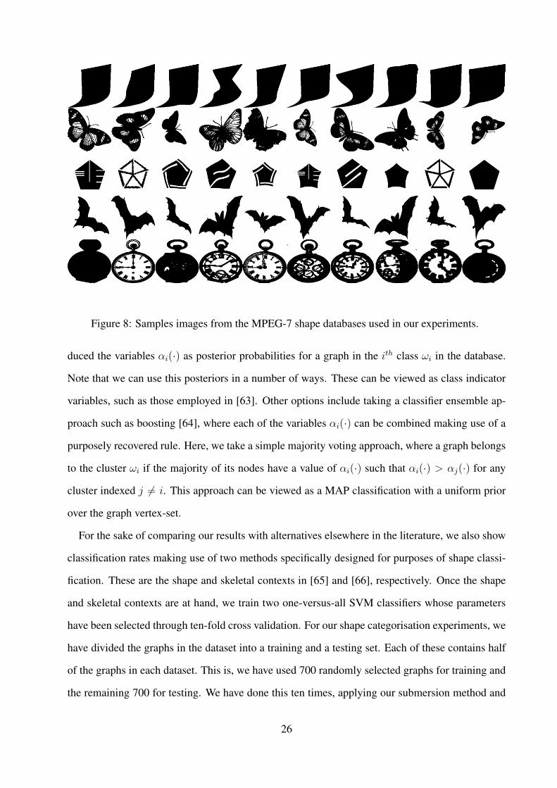
Figure 8: Samples images from the MPEG-7 shape databases used in our experiments.

duced the variables αi(·) as posterior probabilities for a graph in the ith class ωi in the database.

Note that we can use this posteriors in a number of ways. These can be viewed as class indicator

variables, such as those employed in [63]. Other options include taking a classifier ensemble ap-

proach such as boosting [64], where each of the variables αi(·) can be combined making use of a

purposely recovered rule. Here, we take a simple majority voting approach, where a graph belongs

to the cluster ωi if the majority of its nodes have a value of αi(·) such that αi(·) > αj(·) for any

cluster indexed j 6= i. This approach can be viewed as a MAP classification with a uniform prior

over the graph vertex-set.

For the sake of comparing our results with alternatives elsewhere in the literature, we also show

classification rates making use of two methods specifically designed for purposes of shape classi-

fication. These are the shape and skeletal contexts in [65] and [66], respectively. Once the shape

and skeletal contexts are at hand, we train two one-versus-all SVM classifiers whose parameters

have been selected through ten-fold cross validation. For our shape categorisation experiments, we

have divided the graphs in the dataset into a training and a testing set. Each of these contains half

of the graphs in each dataset. This is, we have used 700 randomly selected graphs for training and

the remaining 700 for testing. We have done this ten times, applying our submersion method and

26

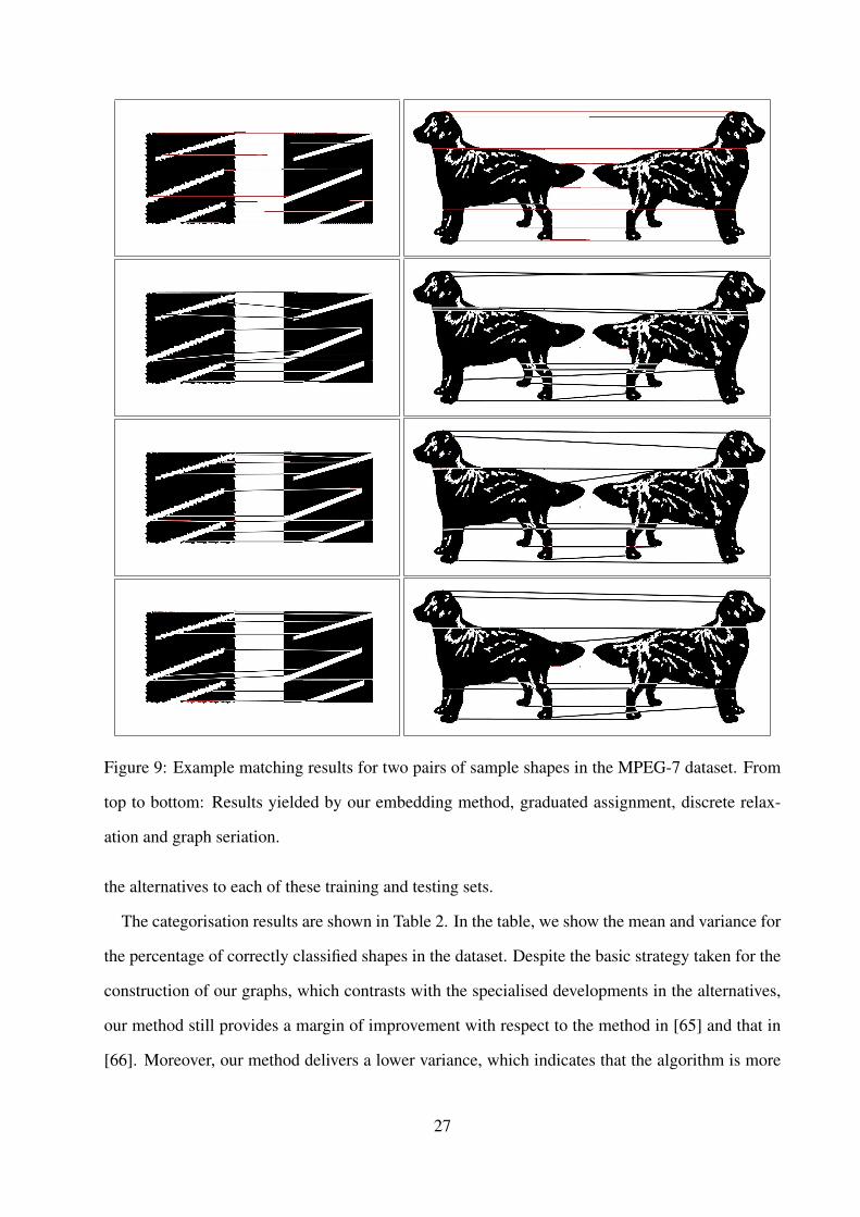
Figure 9: Example matching results for two pairs of sample shapes in the MPEG-7 dataset. From

top to bottom: Results yielded by our embedding method, graduated assignment, discrete relax-

ation and graph seriation.

the alternatives to each of these training and testing sets.

The categorisation results are shown in Table 2. In the table, we show the mean and variance for

the percentage of correctly classified shapes in the dataset. Despite the basic strategy taken for the

construction of our graphs, which contrasts with the specialised developments in the alternatives,

our method still provides a margin of improvement with respect to the method in [65] and that in

[66]. Moreover, our method delivers a lower variance, which indicates that the algorithm is more

27

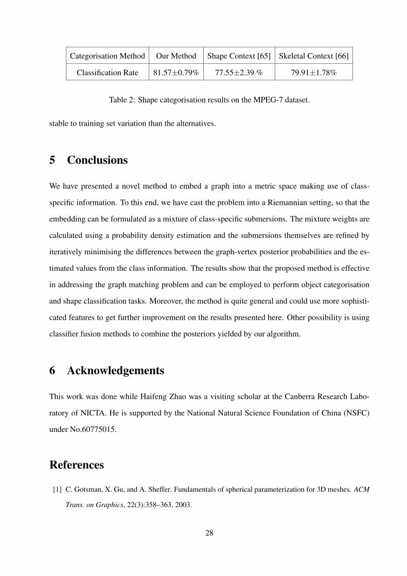
Categorisation Method Our Method Shape Context [65] Skeletal Context [66]

Classification Rate 81.57±0.79% 77.55±2.39 % 79.91±1.78%

Table 2: Shape categorisation results on the MPEG-7 dataset.

stable to training set variation than the alternatives.

5 Conclusions

We have presented a novel method to embed a graph into a metric space making use of class-

specific information. To this end, we have cast the problem into a Riemannian setting, so that the

embedding can be formulated as a mixture of class-specific submersions. The mixture weights are

calculated using a probability density estimation and the submersions themselves are refined by

iteratively minimising the differences between the graph-vertex posterior probabilities and the es-

timated values from the class information. The results show that the proposed method is effective

in addressing the graph matching problem and can be employed to perform object categorisation

and shape classification tasks. Moreover, the method is quite general and could use more sophisti-

cated features to get further improvement on the results presented here. Other possibility is using

classifier fusion methods to combine the posteriors yielded by our algorithm.

6 Acknowledgements

This work was done while Haifeng Zhao was a visiting scholar at the Canberra Research Labo-

ratory of NICTA. He is supported by the National Natural Science Foundation of China (NSFC)

under No.60775015.

References

[1] C. Gotsman, X. Gu, and A. Sheffer. Fundamentals of spherical parameterization for 3D meshes. ACM

Trans. on Graphics, 22(3):358–363, 2003.

28

[2] I. Borg and P. Groenen. Modern Multidimensional Scaling, Theory and Applications. Springer Series

in Statistics. Springer, 1997.

[3] G. Di Battista, P. Eades, R. Tamassia, and I. Tollis. Graph Drawing: Algorithms for the Visualization

of Graphs. Prentice Hall, 1998.

[4] M. F. Demirci, A. Shokoufandeh, S. Dickinson, Y. Keselman, and L. Bretzner. Many-to-many feature

matching using spherical coding of directed graphs. In ECCV04, pages I: 322–335, 2004.

[5] H. Busemann. The geometry of geodesics. Academic Press, 1955.

[6] A. Ranicki. Algebraic l-theory and topological manifolds. Cambridge University Press, 1955.

[7] J. B. Tenenbaum, V. de Silva, and J. C. Langford. A global geometric framework for nonlinear dimen-

sionality reduction. Science, 290(5500):2319–2323, 2000.

[8] S. T. Roweis and L. K. Saul. Nonlinear dimensionality reduction by locally linear embedding. Science,

290:2323–2326, 2000.

[9] M. Belkin and P. Niyogi. Laplacian eigenmaps and spectral techniques for embedding and clustering.

In Neural Information Processing Systems, number 14, pages 634–640, 2002.

[10] T. Cootes, C. Taylor, D. Cooper, and J. Graham. Active shape models - their training and application.

Computer Vision and Image Understanding, 61(1):38–59, 1995.

[11] P. Torr and D. W. Murray. The development and comparison of robust methods for estimating the

fundamental matrix. International Journal of Computer Vision, 24:271–300, 1997.

[12] L. Shapiro and J. M. Brady. Feature-based correspondance - an eigenvector approach. Image and

Vision Computing, 10:283–288, 1992.

[13] S. Ullman. Filling in the gaps: the shape of subjective contours and a model for their generation.

Biological Cybernetics, 25:1–6, 1976.

[14] S. Gold and A. Rangarajan. A graduated assignment algorithm for graph matching. PAMI, 18(4):377–

388, April 1996.

29

[15] A. K. C. Wong and M. You. Entropy and distance of random graphs with application to structural

pattern recognition. IEEE Transactions on Pattern Analysis and Machine Intelligence, 7:599–609,

1985.

[16] W. J. Christmas, J. Kittler, and M. Petrou. Structural matching in computer vision using probabilistic

relaxation. IEEE Transactions on Pattern Analysis and Machine Intelligence, 17(8):749–764, 1995.

[17] R.C. Wilson and E. R. Hancock. Structural matching by discrete relaxation. IEEE Transactions on

Pattern Analysis and Machine Intelligence, 19(6):634–648, June 1997.

[18] T. Caetano, L. Cheng, Q. Le, and A. Smola. Learning graph matching. In Proceedings of the 11th

International Conference on Computer Vision, pages 14–21, 2007.

[19] Fan R. K. Chung. Spectral Graph Theory. American Mathematical Society, 1997.

[20] S. Umeyama. An eigen decomposition approach to weighted graph matching problems. PAMI,

10(5):695–703, September 1988.

[21] G. Scott and H. Longuet-Higgins. An algorithm for associating the features of two images. In Pro-

ceedings of the Royal Society of London, number 244 in B, pages 21–26, 1991.

[22] Bin Luo and E. R. Hancock. Structural graph matching using the EM algorithm and singular value

decomposition. IEEE Trans. on Pattern Analysis and Machine Intelligence, 23(10):1120–1136, 2001.

[23] T.M. Caelli and S. Kosinov. An eigenspace projection clustering method for inexact graph matching.

PAMI, 26(4):515–519, April 2004.

[24] A. Robles-Kelly and E. R. Hancock. A riemannian approach to graph embedding. Pattern Recognition,

40(3):1042–1056, 2007.

[25] A. Sanfeliu and K. S. Fu. A distance measure between attributed relational graphs for pattern recogni-

tion. IEEE Transactions on Systems, Man and Cybernetics, 13:353–362, 1983.

[26] M. A. Eshera and K. S. Fu. A graph distance measure for image analysis. IEEE Transactions on

Systems, Man and Cybernetics, 14:398–407, 1984.

[27] L. G. Shapiro and R. M. Haralick. A metric for comparing relational descriptions. IEEE Trans on

Patterna Analysis and Machine Intelligence, pages 90–94, 1985.

30

[28] R. Myers, R. C. Wilson, and E. R. Hancock. Bayesian graph edit distance. PAMI, 22(6):628–635, June

2000.

[29] S. V. Rice, H. Bunke, and T. A. Nartker. Classes of cost functions for string edit distance. Algorithmica,

18:271–280, 1997.

[30] T. B. Sebastian, P. N. Klein, and B. B. Kimia. Shock-based indexing into large shape databases. In

European Conference on Conputer Vision, volume 3, pages 731–746, 2002.

[31] R. Horaud and T. Skordas. Stereo correspondence through feature grouping and maximal cliques.

IEEE Transactions on Pattern Analysis and Machine Intelligence, 11(11):1168–1180, 1989.

[32] R. Levinson. Pattern associativity and the retrieval of semantic networks. Comput. Math. Appl.,

23:573–600, 1992.

[33] G. Levi. A note on the derivation of maximal common subgraphs of two directed or undirected graphs.

Calcols, 9:341–354, 1972.

[34] J. J. McGregor. Backtrack search algorithms and the maximal common subgraph problem. Software

Practice and Experience, 12:23–34, 1982.

[35] B. T. Messmer and H. Bunke. A decision tree approach to graph and subgraph isomorphism detection.

Pattern Recognition, 32(12):1979–1998, December 1999.

[36] I. Chavel. Riemannian Geometry: A Modern Introduction. Cambridge University Press, 1995.

[37] P. Absil, R. Mahony, and R. Sepulchre. Optimization Algorithms on Matrix Manifolds. Princeton

University Press, 2008.

[38] S. I. Amari and H. Nagaoka. Methods of Information Geometry. Oxford University Press, 2007.

[39] J.L. Gross and T.W. Tucker. Topological graph theory. Wiley Interscience, 1987.

[40] R. Hartshorne. Algebraic Geometry. Springer-Verlag, 1977.

[41] R. O. Duda and P. E. Hart. Pattern Classification. Wiley, 2000.

[42] D. Marquardt. An algorithm for least-squares estimation of nonlinear parameters. SIAM Journal on

Applied Mathematics, 11:431–441, 1963.

31

[43] J. Nocedal and S. Wright. Numerical Optimization. Springer, 2000.

[44] Kenneth Levenberg. A method for the solution of certain non-linear problems in least squares. The

Quarterly of Applied Mathematics, (2):164–168, 1944.

[45] K. Fukunaga. Introduction to Statistical Pattern Recognition. Academic Press, second edition, 1990.

[46] P. J. Ryan. Euclidean and non-Euclidean geometry: an analytical approach. Cambridge University

Press, 1986.

[47] D. W. Scott and S. R. Sain. Multi-dimensional density estimation. Handbook of Statistics—Vol 23:

Data Mining and Computational Statistics, pages 229–263, 2004.

[48] L. Breiman, W. Meisel, and E. Purcell. Variable kernel estimates of multivariate densities. Technomet-

rics, 19:353360, 1977.

[49] P. Bremaud. Markov Chains, Gibbs Fields, Monte Carlo Simulation and Queues. Springer, 2001.

[50] P. Kohli and P. Torr. Efficiently solving dynamic markov random fields using graph cuts. In Proc. of

the IEEE International Conference on Computer Vision, 2005.

[51] B. Taskar, V. Chatalbashev, and D. Koller. Learning associative markov networks. In Proceedings of

the twenty-first international conference on Machine learning, 2004.

[52] Y. LeCun, L. Bottou, Y. Bengio, and P. Haffner. Gradient-based learning applied to document recog-

nition. In Proceedings of the IEEE, volume 86, pages 2278–2324, 1998.

[53] E. R. Hancock and J. V. Kittler. Discrete relaxation. Pattern Recognition, 23:711–733, 1990.

[54] A. Robles-Kelly and E. R. Hancock. Graph edit distance from spectral seriation. Trans. on Pattern

Analysis and Machine Intelligence, 27(3):365–378, 2005.

[55] M. Tuceryan and T. Chorzempa. Relative sensitivity of a family of closest-point graphs in computer

vision applications. Pattern Recognition, 24(5):361–373, 1991.

[56] H. Li, T. Jiang, and K. Zhang. Efficient and robust feature extraction by maximum margin criterion.

In Neural Information Processing Systems, volume 16, 2003.

[57] R. O. Duda and P. E. Hart. Pattern Classification and Scene Analysis. Wiley, 1973.

32

[58] N. Otsu. A thresholding selection method from gray-level histobrams. IEEE Trans. on Systems, Man,

and Cybernetics, 9(1):62–66, 1979.

[59] S. Huwer and H. Niemann. 2d-object tracking based on projection-histograms. In European Conf. on

Computer Vision, pages 861–876, 1998.

[60] Z-H. Zhou and J-M. Xu. On the relation between multi-instance learning and semi-supervised learning.

In Intl. Conf. Machine Learning, pages 1167–1174, 2007.

[61] L. J. Latecki, R. Lakamper, and U. Eckhardt. Shape descriptors for non-rigid shapes with a single

closed contour. In IEEE Conf. on Computer Vision and Pattern Recognition, pages 424–429, 2000.

[62] L. Fei-Fei and P. Perona. A bayesian hierarchical model for learning natural scene categories. In

Comp. Vision and Pattern Recognition, pages II:524–531, 2005.

[63] A. Robles-Kelly and E. R. Hancock. An expectation-maximisation framework for segmentation and

grouping. Image and Vision Computing, 20(9-10):725–738, 2002.

[64] Y. Freund and R. E. Schapire. A decision-theoretic generalization of on-line learning and an application

to boosting. Journal of Computer and System Sciences, 55(1):119–139, 1997.

[65] S. Belongie, J. Malik, and J. Puzicha. Shape matching and object recognition using shape contexts.

IEEE Transactions on Pattern Analysis and Machine Intelligence, 24(4):509–522, 2002.

[66] J. Xie and M. Shah P. Heng. Shape matching and modeling using skeletal context. Pattern Recognition,

41(5):1756–1767, 2008.

33