Graduate School ETD Form 9 (Revised 12/07)

PURDUE UNIVERSITY GRADUATE SCHOOL

Thesis/Dissertation Acceptance

This is to certify that the thesis/dissertation prepared

By

Entitled

For the degree of

Is approved by the final examining committee:

Chair

To the best of my knowledge and as understood by the student in the Research Integrity and Copyright Disclaimer (Graduate School Form 20), this thesis/dissertation adheres to the provisions of Purdue University’s “Policy on Integrity in Research” and the use of copyrighted material.

Approved by Major Professor(s): ____________________________________

____________________________________

Approved by: Head of the Graduate Program Date

Fahmida Ferdous

On Chip Frequency Comb: Characterization and Optical Arbitrary Waveform Generation

Doctor of Philosophy

ANDREW M. WEINER

MINGHAO QI

MUHAMMAD A. ALAM

VLADIMIR M. SHALAEV

ANDREW M. WEINER

M. R. Melloch 10-03-2012

Graduate School Form 20

(Revised 9/10)

PURDUE UNIVERSITY GRADUATE SCHOOL

Research Integrity and Copyright Disclaimer

Title of Thesis/Dissertation:

For the degree of Choose your degree

I certify that in the preparation of this thesis, I have observed the provisions of Purdue University

Executive Memorandum No. C-22, September 6, 1991, Policy on Integrity in Research.*

Further, I certify that this work is free of plagiarism and all materials appearing in this

thesis/dissertation have been properly quoted and attributed.

I certify that all copyrighted material incorporated into this thesis/dissertation is in compliance with the

United States’ copyright law and that I have received written permission from the copyright owners for

my use of their work, which is beyond the scope of the law. I agree to indemnify and save harmless

Purdue University from any and all claims that may be asserted or that may arise from any copyright

violation.

______________________________________ Printed Name and Signature of Candidate

______________________________________ Date (month/day/year)

*Located at http://www.purdue.edu/policies/pages/teach_res_outreach/c_22.html

On Chip Frequency Comb: Characterization and Optical Arbitrary Waveform Generation

Doctor of Philosophy

Fahmida Ferdous

03-29-2012

ON CHIP FREQUENCY COMB: CHARACTERIZATION AND OPTICAL

ARBITRARY WAVEFORM GENERATION

A Dissertation

Submitted to the Faculty

of

Purdue University

by

Fahmida Ferdous

In Partial Fulfillment of the

Requirements for the Degree

of

Doctor of Philosophy

December 2012

Purdue University

West Lafayette, Indiana

ii

In memory of

Hosne Ara

my mother and my best friend

and

Ferdous Alam

my beloved husband

iii

ACKNOWLEDGMENTS

First, I want to thank my advisor Prof A. M. Weiner for his continuous advice,

suggestions and support throughout this amazing journey of knowledge. It was a

great exciting and pleasant opportunity to be a member of his group, to learn from

him and to do research on very interesting topics.

I specially thank Dr. D. E. Leaird who made the complex experimental procedure

easy and always there when I needed any technical support. I would like to thank

my Ph.D. committee members and colleagues for valuable discussions. I would like to

thank Dee Dee Dexter for invaluable help on official matters. I would also thank our

collaborators Dr. H. Miao, Dr. K. Srinivasan and Dr. V. Aksyuk at NIST, Gaithers-

burg, MD for the silicon nitride ring fabrication and valuable technical discussion and

guideline.

I express my deep gratitude to my parents, my brothers and sister who always

supported and encouraged me throughout my life and study. They always were on

my side in my good and bad times. Although, nothing I could write would be enough

to express my appreciations to my family, I can not resist writing a few words to show

my deep appreciation to my husband Dr. Ferdous Alam who gave me suggestions

and encouragements from time to time and always supported me mentally; and my

baby boy Raed Alam whose heavenly smiles always make my world wonderful.

I appreciate all my good purdue friends who made purdue life nice and warm which

help me to stay focused in my research. I really appreciate the dinner invitations and

crone maize outing with Prof Weiner and Brenda Weiner’s family which always refresh

me to start my research with full energy and enthusiasm.

iv

TABLE OF CONTENTS

Page

LIST OF TABLES . . . . . . . . . . . . . . . . . . . . . . . . . . . . . . . . vi

LIST OF FIGURES . . . . . . . . . . . . . . . . . . . . . . . . . . . . . . . vii

ABSTRACT . . . . . . . . . . . . . . . . . . . . . . . . . . . . . . . . . . . xiii

1 INTRODUCTION . . . . . . . . . . . . . . . . . . . . . . . . . . . . . . 1

1.1 Optical frequency comb . . . . . . . . . . . . . . . . . . . . . . . . . 1

1.2 Optical arbitary waveform generation . . . . . . . . . . . . . . . . . 3

1.3 Optical waveguide . . . . . . . . . . . . . . . . . . . . . . . . . . . . 6

1.4 optical resonator . . . . . . . . . . . . . . . . . . . . . . . . . . . . 7

1.5 Organization of the thesis . . . . . . . . . . . . . . . . . . . . . . . 8

2 DUAL COMB ELECTRIC FIELD CROSS-CORRELATION TECHNIQUE 10

2.1 Introduction . . . . . . . . . . . . . . . . . . . . . . . . . . . . . . . 10

2.2 Conventional EFXC and Dual Comb EFXC . . . . . . . . . . . . . 11

2.3 Experimental set up and Data processing . . . . . . . . . . . . . . . 12

2.4 Results . . . . . . . . . . . . . . . . . . . . . . . . . . . . . . . . . . 17

2.5 Future work . . . . . . . . . . . . . . . . . . . . . . . . . . . . . . . 18

3 SPECTRAL LINE-BY-LINE PULSE SHAPING OF AN ON-CHIP MI-CRORESONATOR FREQUENCY COMB . . . . . . . . . . . . . . . . 19

3.1 Introduction . . . . . . . . . . . . . . . . . . . . . . . . . . . . . . . 19

3.2 Four wave mixing and comb generation . . . . . . . . . . . . . . . . 19

3.3 On chip frequency comb characterization . . . . . . . . . . . . . . . 24

3.4 Si3N4 ring and Experiment setup . . . . . . . . . . . . . . . . . . . 25

3.5 Results . . . . . . . . . . . . . . . . . . . . . . . . . . . . . . . . . . 27

3.6 Device fabrication . . . . . . . . . . . . . . . . . . . . . . . . . . . . 39

3.7 Experimental procedure . . . . . . . . . . . . . . . . . . . . . . . . 43

v

Page

3.8 Simulation . . . . . . . . . . . . . . . . . . . . . . . . . . . . . . . . 44

3.9 Conclusion . . . . . . . . . . . . . . . . . . . . . . . . . . . . . . . . 48

4 TIME DOMAIN COHERENCE STUDY OF SILICON NITRIDE MICRORES-ONATOR FREQUENCY COMBS . . . . . . . . . . . . . . . . . . . . . 49

4.1 Introduction . . . . . . . . . . . . . . . . . . . . . . . . . . . . . . . 49

4.2 Si3N4 ring and experimental setup . . . . . . . . . . . . . . . . . . . 53

4.3 Results . . . . . . . . . . . . . . . . . . . . . . . . . . . . . . . . . . 54

4.4 Visibility curves . . . . . . . . . . . . . . . . . . . . . . . . . . . . . 57

4.5 Conclusion . . . . . . . . . . . . . . . . . . . . . . . . . . . . . . . . 67

5 FUTURE WORK . . . . . . . . . . . . . . . . . . . . . . . . . . . . . . . 68

5.1 Intoduction . . . . . . . . . . . . . . . . . . . . . . . . . . . . . . . 68

5.2 Future work . . . . . . . . . . . . . . . . . . . . . . . . . . . . . . . 68

5.2.1 SHG Frequency-resolved optical gating . . . . . . . . . . . . 68

5.2.2 Comb improvement and dispersion measurement . . . . . . . 70

5.3 RF beating experiment . . . . . . . . . . . . . . . . . . . . . . . . . 73

5.4 Pulse generation from Kerr combs . . . . . . . . . . . . . . . . . . . 76

5.5 On-chip pulsed light source . . . . . . . . . . . . . . . . . . . . . . . 79

LIST OF REFERENCES . . . . . . . . . . . . . . . . . . . . . . . . . . . . 81

VITA . . . . . . . . . . . . . . . . . . . . . . . . . . . . . . . . . . . . . . . 86

vi

LIST OF TABLES

Table Page

3.1 Summary of groups working on Comb generation . . . . . . . . . . . . 21

vii

LIST OF FIGURES

Figure Page

1.1 Schematic diagram (a) Ideal frequency comb, (b) Representative outputspectrum of a mode locked laser with a Gaussian envelope, (c) correspond-ing time domain representation [3]. . . . . . . . . . . . . . . . . . . . . 2

1.2 Schematic diagram of pulse shaping (a) Group of lines regime, (b) Line-by-line regime [6]. . . . . . . . . . . . . . . . . . . . . . . . . . . . . . 4

1.3 OAWG with frame to frame update [7]. . . . . . . . . . . . . . . . . . . 4

1.4 Pulse shaper [3]. . . . . . . . . . . . . . . . . . . . . . . . . . . . . . . 5

1.5 Light propagation in fiber [9]. . . . . . . . . . . . . . . . . . . . . . . . 6

2.1 Schematic of experimental setup. Here ∆fCEO is 100 MHz; fsig is 9.953GHz; fref is fsig +∆frep; ∆frep is 220 KHz. CW: continuous-wave laser;PM: phase modulator; IM: intensity modulator; Amp: optical amplifier;PD: photo detector; AO: acousto-optic frequency shifter. . . . . . . . . 12

2.2 (a) EFXC data for bandwidth-limited signal showing multiple periods,(b)EFXC data for bandwidth-limited signal zoomed-in to show the fringeperiod, (c) EFXC data for π phase step signal, and (d) EFXC data forcubic phase signal. . . . . . . . . . . . . . . . . . . . . . . . . . . . . . 14

2.3 (Color online) Retrieved (a) amplitude and phase for (b) approximatelybandwidth-limited signal, (c) quadratic phase, (d) cubic phase, (e) πphase step signals obtained via pulse shaper, and (f) after propagationthrough 20 km optical fiber. In (b) 9 sets of data are overlaid. Circles(c-f): retrieved phase; lines: applied phase through pulse shaper (c-e) andquadratic fit (f). . . . . . . . . . . . . . . . . . . . . . . . . . . . . . . 16

3.1 Optical frequency comb generation in a micro resonator. (a) shows theresonator and the output comb spectrum. The individual comb modesare spaced by FSR of the cavity. (b) shows the principle of the combgeneration process. Degenerate and nondegenerate FWM allow conversionof a CW laser into an optical frequency comb [37]. . . . . . . . . . . . 23

3.2 The role of dispersion in comb generation. Due to the dispersion in thecavity, FSR varies with the optical frequency, so that the cavity resonancesare not spaced equally in frequency. The generated optical frequency comb(lines), in contrast, is perfectly equidistant [55]. . . . . . . . . . . . . . 24

viii

Figure Page

3.3 (a) Microscope image of a 40 µm radius microring with the coupling region.(b) Image of a fiber pigtail. (c) Transmission spectrum of the microringresonator. (d) Zoomed in spectrum of an optical mode with a 1.2 pmlinewidth. . . . . . . . . . . . . . . . . . . . . . . . . . . . . . . . . . . 26

3.4 Scheme of the experimental setup for line-by-line pulse shaping of a fre-quency comb from a silicon nitride microring. CW: continuous-wave;EDFA: erbium doped fiber amplifier; FPC: fiber polarization controller;µring: silicon nitride microring; OSA: optical spectrum analyzer. . . . 27

3.5 Spectra of generated optical frequency combs. For each spectrum the CWpump wavelength, estimated power coupled to the access waveguide, andring radius will be succinctly indicated (a) 1543.07 nm, 0.45 W , 40 µm;(b) 1548.63 nm, 66 mW, 100 µm; (c) 1547.15 nm, 1.4 W, 200 µm; (d)1549.26 nm, 1.4 W, 200 µm; (e) 1551.67 nm, 1.4 W, 100 µm; and (f)1551.74 nm, 1.4 W, 100 µm. . . . . . . . . . . . . . . . . . . . . . . . 29

3.6 Spectra of generated optical frequency combs. CW pump wavelengths areindicated in the figures. All the spectrums are taken from the same 200µmradius ring with 500 nm gap between ring and waveguide. The CW powerand other experimental parameters remains same (1.1 W). . . . . . . . 30

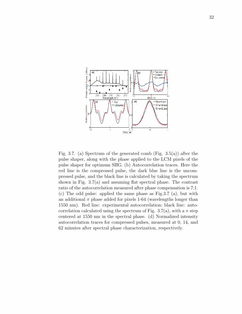
3.7 (a) Spectrum of the generated comb (Fig. 3.5(a)) after the pulse shaper,along with the phase applied to the LCM pixels of the pulse shaper for opti-mum SHG. (b) Autocorrelation traces. Here the red line is the compressedpulse, the dark blue line is the uncompressed pulse, and the black line iscalculated by taking the spectrum shown in Fig. 3.7(a) and assuming flatspectral phase. The contrast ratio of the autocorrelation measured afterphase compensation is 7:1. (c) The odd pulse: applied the same phase asFig.3.7 (a), but with an additional π phase added for pixels 1-64 (wave-lengths longer than 1550 nm). Red line: experimental autocorrelation;black line: autocorrelation calculated using the spectrum of Fig. 3.7(a),with a π step centered at 1550 nm in the spectral phase. (d) Normalizedintensity autocorrelation traces for compressed pulses, measured at 0, 14,and 62 minutes after spectral phase characterization, respectively. . . 32

ix

Figure Page

3.8 (a) and (b) Spectra of the generated combs (corresponding to Fig. 3.5(c)and 3.5(b), respectively) after the pulse shaper, along with the phase ap-plied to the LCM pixels for optimum SHG signals. (c) and (d) Autocorre-lation traces corresponding to (a) and (b). Red lines are the compressedpulses after phase correction, dark blue lines are the uncompressed pulses,and black lines are calculated by taking the spectra shown in (a) and (b)and assuming flat spectral phase. The contrast ratios of the autocorrela-tions measured after phase compensation are 14:1 and 12:1, respectively.Here Light gray traces show the range of simulated autocorrelation traces. 34

3.9 Schematic diagram of frequency instability due to uncorrelated line-to-linerandom phase. Here red arrow shows the effect of δfn. δfn is the smallfixed shifts (assumed to be random and uncorrelated) of the individualfrequencies from their ideal, evenly spaced positions. . . . . . . . . . . 36

3.10 Theoretical traces for nonlinear SHG autocorrelation measurements [18,61]. The contrast ratio is 2:1 for continuous noise and 2:1:0 for a finiteduration noise burst. A single coherent pulse decays smoothly to zerobackground level. The pulse duration can be estimate from the full widthhalf maximum (FWHM) ∆τ of the correlation trace G2(τ). . . . . . . . 37

3.11 (a), (b) and (c) Spectra of the generated comb (corresponding to Fig.3.5(d), 3.5(e) and 3.5(f), respectively) after the pulse shaper, along withphase applied to the LCM pixels for optimum SHG signals. (d), (e) and(f) Autocorrelation traces corresponding to (a), (b) and (c). Red linesare the compressed pulse after phase correction, dark blue lines are theuncompressed pulse, and black lines are the calculated trace by taking thespectrum shown in (a), (b) and (c) and assuming flat spectral phase. HereLight gray traces show the range of simulated autocorrelation traces. . 40

3.12 (a) Spectrum of the generated comb (Fig. 3.5(f)) after the pulse shaper,along with the phase applied to the LCM pixels of the pulse shaper foroptimum SHG. (b) Autocorrelation traces. Here the red line is the com-pressed pulse, the dark blue line is the uncompressed pulse, and the blackline is calculated by taking the spectrum shown in Fig. 3.12(a) and as-suming flat spectral phase. (c) The odd pulse: applied the same phase asFig. 3.12(a), but with an additional π phase added for wavelengths longerthan 1554 nm. Red line: experimental autocorrelation; black line: auto-correlation calculated using the spectrum of Fig. 3.12(a), with a π stepcentered at 1555 nm in the spectral phase. Figs. 3.11(c)(f) are repeatedas Figs. 3.12 (a)(b). . . . . . . . . . . . . . . . . . . . . . . . . . . . . 41

x

Figure Page

3.13 (a)Si3N4 microring. (b)V groove (left rectangular shape) is connected toinverse tapered waveguide. (c)SEM of the wave guide (d) SEM of the Vgroove. . . . . . . . . . . . . . . . . . . . . . . . . . . . . . . . . . . . . 42

3.14 Simulated intensity autocorrelation traces in which uncorrelated randomspectral phases are uniformly distributed in the range 0 to ∆φ, for variousvalues of ∆φ. The experimental autocorrelation trace from Fig. 3.11(f) isalso plotted (black line). . . . . . . . . . . . . . . . . . . . . . . . . . . 46

3.15 Selected simulated intensity profiles with uncorrelated random spectralphases that are uniformly distributed in the range 0 to ∆φ = 0.8π. Theseplots are normalized to the peak intensity calculated for the case of 0 phasefluctuations. . . . . . . . . . . . . . . . . . . . . . . . . . . . . . . . . . 47

4.1 Possible routes to comb formation. The optical frequency axis is portrayedin free spectral range (FSR) units. Arrows are drawn in an attempt torepresent the approximate order in which new comb lines are generated;no attempt is made to indicate all the couplings involved in the four wavemixing process. (a) Case where initial comb lines are spaced by one FSRfrom the pump line, with subsequent comb lines, generated through cas-caded four wave mixing, spreading out from the center. (b) Case whereinitial comb lines are spaced from the pump line by N FSRs, where N>1is an integer. Here N=3 is assumed. (c) When the pump laser is tunedcloser into resonance, additional lines are observed to fill in, resulting inspectral lines spaced by nominally 1 FSR. . . . . . . . . . . . . . . . . 52

4.2 a) Spectrum of the generated 3 FSR spacing comb after the pulse shaper.(b) Autocorrelation traces corresponding to (a). (c) Spectrum of the gen-erated 1 FSR spacing comb after the pulse shaper. Here we tune the CWlaser 53 pm towards the red side than that of (a). (d) Autocorrelationtraces corresponding to (c). . . . . . . . . . . . . . . . . . . . . . . . . 55

4.3 Spectra and autocorrelation traces for 3 subfamilies of comb lines with 3FSR spacing selected from the spectrum shown in Fig. 4.2(c). Blue andred traces are experimental traces before and after phase compensationrespectively. Black traces are calculated by taking the OSA spectrumsand assuming flat spectral phase. . . . . . . . . . . . . . . . . . . . . . 56

4.4 Spectra and autocorrelation traces for 2 subfamilies of comb lines with 2FSR spacing selected from the spectrum shown in Fig. 4.2(c). Blue andred traces are experimental traces before and after phase compensationrespectively. Black traces are calculated by taking the OSA spectrumsand assuming flat spectral phase. . . . . . . . . . . . . . . . . . . . . . 58

xi

Figure Page

4.5 Autocorrelation traces for 3 line experiments for different ∆φ for lines{−3, 0, 3}, for which high coherence is observed. Here colored lines arethe experimental traces and black lines are the simulated traces. . . . . 59

4.6 Autocorrelation traces for 3 line experiments for different ∆φ for lines{−2, 1, 4}, for which low coherence is observed. Here colored lines are theexperimental traces and black lines are the simulated traces. . . . . . . 60

4.7 Autocorrelation traces for 3 line experiments for different ∆φ for lines{−7,−4,−1}, for which low coherence is observed. Here colored lines arethe experimental traces and black lines are the simulated traces. . . . . 61

4.8 Visibility traces of (a) three subfamilies of 3 FSRs, (b) two subfamilies of2 FSRs, and (c) two subfamilies of 1 FSR. Here in the visibility curves,red, green and black lines are the experimental data; blue lines are idealtheoretical curves calculated assuming full coherence based on the powerspectra corresponding to the respective red line visibility curves. Num-bers in curly braces indicate the 3 lines that are used in the experiments.Error bars (shown for representative curves) and shaded areas representthe mean ± one standard deviation. . . . . . . . . . . . . . . . . . . . . 63

4.9 Proposed model for type II comb formation. (a) First: generation of a cas-cade of sidebands spaced by N FSRs (Nδω) from the pump. Here N=6 isillustrated. (b)-(c) The 2nd event is an independent four-wave mixing pro-cess, which creates new sidebands spaced by a different amount,±nδω′(n=1,2or 3....for different lines), from each of the lines in the previous step. Dueto dispersion, it is very unlikely that the new frequency spacings will beexact submultiples of the original N FSR spacing; i.e.,δω

′ 6= δω. . . . . 66

5.1 Polarization insensitive ultra low-power SHG FROG setup [65]. . . . . 69

5.2 The model used for simulation. Here h,b and w are the height, base of theSi3N4 and cladding layer(SiO2) dimension respectively. . . . . . . . . . 71

5.3 Simulation results of the present device. Here h,b and θ are the height,base and angle from the vertical direction of the Si3N4 respectively. . . 72

5.4 Schematic diagram of the experimental setup for dispersion calculation.Here OPO: optical parametric osillator; DUT: device under test. . . . . 73

5.5 Simulation results with various dimensions to find optimum device dimen-sion for next generation device. Here h,b and θ are the height, base andangle from the vertical direction of the Si3N4 respectively. . . . . . . . 74

5.6 (a) Schematic diagram for RF beating experiment. (b) expected results:One line will be beat with tunable laser and multiple lines will be seen inRF spectrum analyzer. . . . . . . . . . . . . . . . . . . . . . . . . . . . 75

xii

Figure Page

5.7 High coherent temporal case: (a) Spectrum of the generated comb afterthe pulse shaper with applied phases. (b) Autocorrelation traces. Herered line is the experimental AC trace when we apply red dot phases ofFig 5.7(a). Black line is the calculated AC considering spectrum shownin Fig 5.7(a) and assuming spectrum flat spectral phases. Blue line isthe experimental AC trace without pulse compression. Green line is theexperimental AC trace when we apply green dot phases of Fig 5.7(a). 77

5.8 Partial coherent temporal case: (a) Spectrum of the generated comb afterthe pulse shaper with applied phases. (b) Autocorrelation traces. Herered line is the experimental AC trace when we apply red dot phases ofFig 5.8(a). Black line is the calculated AC considering spectrum shownin Fig 5.8(a) and assuming spectrum flat spectral phases. Blue line isthe experimental AC trace without pulse compression. Green line is theexperimental AC trace when we apply green dot phases of Fig 5.8(a). . 78

5.9 Schematic diagram for on-chip pulsed light source. . . . . . . . . . . . . 80

xiii

ABSTRACT

Fahmida Ferdous Ph.D., Purdue University, December 2012. On Chip FrequencyComb: Characterization and Optical Arbitrary Waveform Generation. Major Pro-fessor: Andrew M. Weiner.

Recently, on-chip comb generation methods based on nonlinear optical modula-

tion in ultrahigh quality factor monolithic micro-resonators have been demonstrated.

In these methods, two pump photons are transformed into sideband photons in a four

wave mixing process mediated by the Kerr nonlinearity. The essential advantages

of these methods are simplicity, small size, very high repetition rates and sometimes

CMOS compatibility. We investigate line-by-line pulse shaping of such combs gener-

ated in silicon nitride ring resonators. We demonstrate a simple example of optical

arbitrary waveform generation (OAWG) from Kerr comb. We observe two distinct

paths to comb formation which exhibit strikingly different time domain behaviors.

For combs formed as a cascade of sidebands spaced by a single free spectral range

(FSR) that spread from the pump, we are able to compress to nearly bandwidth-

limited pulses. This indicates high coherence across the spectra and provides new

data on the high passive stability of the spectral phase. For combs where the initial

sidebands are spaced by multiple FSRs which then fill in to give combs with single

FSR spacing, the time domain data reveal partially coherent behavior. We also inves-

tigate the behaviors of a few sub-families of the partially coherent combs selected by

a pulse shaper. We observe different coherence properties for different groups of comb

lines. Furthermore we will discuss an ultrafast characterization techniques called dual

comb electric field cross correlation. This linear technique will provide both low op-

tical power and broader bandwidth capability for full time domain characterization

of OAWG from Kerr comb.

1

1. INTRODUCTION

Our research is focused on different aspects of optical arbitrary waveform (OAWG)

such as generation, characterization and applications. OAWG is a very powerful tool

for high precision spectroscopy, broad band gas sensing, optical clock, attosecond

physics and also in RF photonics and in silicon photonics. Before going to deep in

our work, we will discuss some basic things such as optical comb, OAWG, waveguide

and resonator.

1.1 Optical frequency comb

Optical frequency comb consists of periodic discrete spectral lines with fixed fre-

quency positions [1,2]. Frequency comb can be generated in mode locked lasers with

stabilized repetition rates and center frequencies. Attributes that are desirable in a

frequency comb include having stable frequency positions of individual comb lines

and knowing the exact frequency position of the individual comb lines. By suitable

locking mechanisms, the frequency positions of the comb lines can be stabilized, how-

ever exact determination of individual frequencies is hard. This happens because the

absolute optical frequencies constituting the comb will not be exact multiples of the

repetition rate owing to difference between the phase and group velocities in the laser

cavity. The individual comb lines are given by the equation [2]

fm = mfrep + ε (1.1)

where frep is the repetition rate of the laser and ε is known as the carrier envelope

offset, whose value is not easy to obtain and because of which, exact determination

2

Fig. 1.1. Schematic diagram (a) Ideal frequency comb, (b) Repre-sentative output spectrum of a mode locked laser with a Gaussianenvelope, (c) corresponding time domain representation [3].

of frequencies becomes difficult. Fig 1.1 schematically shows this. Fig 1.1(a) shows

an ideal frequency comb with an infinite bandwidth. Fig 1.1(b) shows a schematic

of a realistic spectrum from a mode locked laser with a Gaussian envelope where the

comb lines are offset from multiples of the repetition rate by the carrier envelope off-

set frequency ε. Fig 1.1(c) shows the envelope of time domain trace corresponding to

the comb. In the last decade, driven by metrological applications, there were signifi-

cant developments in frequency combs and methods to measure and lock the carrier

envelope offset was proposed. Such combs are called self referenced frequency combs

and they have stabilized frequency lines with known frequency positions [1, 2]. The

repetition rate can be very small (i.e. GHz) to THz. However, for practical applica-

tions, for e.g. in optical communications, the interesting regime will be in repetition

3

rates of 10s of GHz corresponding to the data rates used. Also, in order to be able to

address individual spectral lines in a pulse shaper, it is necessary to have relatively

wider spacing (again of the order of GHz). So when we refer to OAWG, we are usually

talking about relatively high repetition rate frequency combs. However, mode locked

lasers don’t scale well into these repetition rates while maintaining frequency stabil-

ity. Due to this reason, there has been significant development of alternate frequency

comb sources with high repetition rates [4, 5]. In fact all the frequency comb sources

which we use in our work are novel sources and not mode locked lasers.

1.2 Optical arbitary waveform generation

Utilizing such combs together with the well established techniques of femtosecond

pulse shaping, individual spectral lines can be controlled independently allowing very

high complexity waveform generation. This is known as optical arbitrary waveform

generation (OAWG) and promises to have significant impact in optical science and

technology. By shaping the amplitude and phase of individual lines of a frequency

comb, 100% duty factor waveforms can be generated via OAWG. Figure 1.2 schemat-

ically shows the difference between conventional pulse shaping (group of lines regime)

and OAWG (line-by-line regime). In the group of lines case, in time domain shaped

pulses are isolated in time, where as in the line-by-line regime they occupy the entire

time window leading to 100 % duty factor waveforms. Another interesting extension

of this regime is the case when the pulse shaping operation is modified at the rep-

etition rate of the comb. In this case, the waveform updates on a frame to frame

basis allowing for potentially infinite record length, very high complexity waveforms.

This is schematically shown in fig 1.3. Let us now briefly describe the operating

principle of femtosecond pulse shaping by which the waveforms are generated [8]. In

a Fourier pulse shaping apparatus, the spectrum of an incident pulse is spread spa-

4

Fig. 1.2. Schematic diagram of pulse shaping (a) Group of linesregime, (b) Line-by-line regime [6].

Fig. 1.3. OAWG with frame to frame update [7].

5

Fig. 1.4. Pulse shaper [3].

tially using a spectral disperser (a diffraction grating) and focused onto a spatial light

modulator (SLM), which transfers spatial phase and amplitude information onto the

complex optical spectrum. This Fourier synthesis procedure results, after the optical

frequencies are recombined, in programmable user-defined waveforms. An important

requirement of the OAWG setup is the ability to spectrally resolve individual comb

lines. This can be achieved in conventional grating based pulse shapers using bigger

beams and finer groove spacings on the gratings. Fig 1.4 shows the schematic of a

grating based high resolution pulse shaper aligned in a reflective configuration used

to address comb lines individually.

6

Fig. 1.5. Light propagation in fiber [9].

1.3 Optical waveguide

Silicon photonics is attracting more interest in recent years since it provides a

possible solution for chip-scale high speed data communication, for example, between

two Central Processing Units. Traditional copper transmission line suffers from delay

limitation in high speed data transmission, while optical signal does not have this

problem. The essential advantages of silicon photonics are simplicity, small size, very

low power consumption and CMOS compatibility. Lets first discussed briefly about

the basic building block: waveguides. Waveguides used at optical frequencies are

typically dielectric waveguides, a dielectric material with high permittivity, and thus

high index of refraction, is surrounded by a material with lower permittivity. The

simple way to understand the guides of optical waves is by total internal reflection.

The most common optical waveguide is optical fiber. People can simply understand

the optical fiber in linear propagation approximation as in Fig. 1.5: The optical field

is confined in the high refractive index area. Since the boundary condition is com-

7

plicated now (dielectric waveguide), there is evanescent field decaying exponentially

outside the waveguide boundary. Normally, the waveguide has extremely small inter-

section. The size is so small that automatically kills off the high modes. The benefit

of single mode propagation is to avoid mode dispersion. Every single mode will have

different propagation constant (except degenerate modes). So the optical power in

individual mode travels through the waveguide with different velocity. This is called

mode dispersion. It will broaden the data packet in time domain hence increase the

bit error rate in high speed data transmission. Single mode waveguide will naturally

eliminate the mode dispersion. In most cases we need to couple the optical power

from outside fiber into the waveguide. For single mode optical fiber, the mode profile

is around 10 µm in diameter. In silicon waveguide the mode profile is generally similar

as the waveguide geometry (< 1µm). To match the modes, one strategy is to use a

taper part on chip to match the mode between fiber and waveguide, or inverse taper

or grating-assisted coupling. In our lab we normally used the first two which require

accurate alignment between the fiber and waveguide.

1.4 optical resonator

With the state-of-art fabrication of silicon waveguide, both passive and active

devices are demonstrated on silicon chip with excellent performances. Optical cavities

are one of the most popular devices under research. Optical cavities are a major

component of lasers, surrounding the gain medium and providing feedback of the laser

light. They are also used in optical parametric oscillators and some interferometers.

The functions as filter, modulator, switcher, spectral shaper, sensor and as comb

sources have been investigated profoundly. The typical micro ring resonator is a

compact optical cavity which shows periodical response in spectrum domain. It can

be side coupled by one or two straight waveguide to form a pole-type filter.The cavity

8

contains a dielectric round waveguide or a round disk, where the optical beam can

bounce back and forth at the ring or disk boundary. It is called whispering gallery

mode (WGM). WGMs occur at particular resonant wavelengths of light confined

to a cylindrical or spherical volume with an index of refraction greater than that

surrounding it. At these wavelengths, the light undergoes total internal reflection at

the volume surface and becomes trapped within the volume for timescales of the order

of nanoseconds. Micro ring resonator is a round planar waveguide where the light is

going along the waveguide. No reflection happens. Several schemes can be used to

feed the power into the resonator. The most common way is using coupling between

the micro resonator and waveguide. As introduced in last part the mode propagated

in waveguide has the evanescent field outside the edge. Putting two waveguide very

close would let the power to transfer between two waveguide. In the application where

very high Q is needed, we need to match the coupling strength with the round trip

loss in the resonator. This case is called critical coupling. Following the definition we

call the weaker coupling as under coupling and stronger coupling as over coupling.

By manipulating the coupling strength, we can in some sense tuning the loaded Q

value of resonator with the intrinsic Q value unchanged.

1.5 Organization of the thesis

The dissertation is organized into the following chapters. In chapter 2 we will

discuss a characterization technique for optical arbitrary waveforms based on two fre-

quency combs. We will present one characterization techniques which may be used

in future for characterization of on chip comb. In chapter 3, a novel method which

is recently developed for the generation of the on chip comb will be discussed. Line-

by-line pulse shaping of Kerr combs generated in silicon nitride ring resonators is

discussed. A simple example of optical arbitrary waveform generation (OAWG) from

9

Kerr comb is demonstrated. Two distinct paths to comb formation which exhibit

strikingly different time domain behaviors is observed. In chapter 4, the behaviors of

a few sub-families of the partially coherent combs selected by a pulse shaper is inves-

tigated. Different coherence properties for different groups of comb lines is observed.

In chapter 5, some future directions are discussed.

10

2. DUAL COMB ELECTRIC FIELD

CROSS-CORRELATION TECHNIQUE

2.1 Introduction

The use of a pulse shaper [8] to manipulate optical frequency combs [11, 12] on a

line by line basis, termed optical arbitrary waveform generation [13–15], leads to new

challenges in ultrafast waveform characterization. Waveforms generated through line-

by-line pulse shaping exhibit several unique attributes. Such waveforms may exhibit

100% duty cycle, with shaped waveforms spanning the full time domain repetition pe-

riod of the frequency comb, and with spectral amplitude and phase changing abruptly

from line to line. Although methods for full characterization of ultrashort pulse fields,

such as frequency-resolved optical gating (FROG) and spectral phase interferometry

for direct electrical field reconstruction (SPIDER), are well developed [16–18], such

methods are typically applied to measurement of low duty cycle pulses that are iso-

lated in time, with spectra that are smoothly varying, and with relatively low time-

bandwidth product. Hence new characterization approaches are desired for shaped

waveforms generated from frequency combs. A few techniques for OAWG character-

ization have recently been reported [6, 15, 19, 20]. Some of these techniques require a

series of measurements performed sequentially which limits measurement speed [6,15],

while others require nonlinear optics and/or an array detector [15, 19, 20]. Here we

demonstrate a novel electric field cross-correlation (EFXC) technique in which a pre-

characterized reference comb is used to measure an unknown signal field from a second

optical comb. Although related to standard EFXC techniques, our experiment is con-

0This work is published in [10]

11

structed in a way uniquely suited to characterization of shaped waveforms from comb

sources. Our technique requires only a linear point detector and is simple to con-

struct. It provides both high measurement sensitivity and fast (tens of microseconds)

data acquisition. Our work is closely related to recent coherent multi-heterodyne

spectroscopy experiments in which a pair of stabilized combs is exploited for rapid

measurement of absorption and phase spectra of gas phase samples [21]. Our work

is also related to Linear Optical Sampling [22] which has recently been implemented

with dual self-referenced and stabilized, ∼100 MHz repetition rate comb sources to

achieve 15 bit sampling resolution [23]. An important difference is that our setup

uses simple comb sources based on modulation of a CW laser [4, 24, 25] rather than

octave-spanning self-referenced combs. Our simple combs operate at a relatively high

repetition rate (10 GHz), which is advantageous both for applications in telecommu-

nications and for arbitrary optical waveform generation, and our measurements are

applied to shaped waveform characterization rather than spectroscopy.

2.2 Conventional EFXC and Dual Comb EFXC

EFXC measures the interference between a signal field (as) and reference field

(ar) in the time domain as a function of the relative delay (τ). Traditionally, the

delay is swept using a mechanical translation stage [26]. The resulting time-average

power is recorded using a slow photo-detector as a function of delay and is written as

follows [18]:

< Pout(τ) >=1

2(Us + Ur +

∫{asa∗r(t− τ) exp jω0τ + C.C.}dt). (2.1)

Here Us and Ur are the pulse energies and ωo is the carrier frequency. The unknown

signal pulse can be fully recovered from a known, well characterized reference pulse.

Note that in the traditional scheme, the phase delay and group delay vary at exactly

12

Fig. 2.1. Schematic of experimental setup. Here ∆fCEO is 100 MHz;fsig is 9.953 GHz; fref is fsig +∆frep; ∆frep is 220 KHz. CW:continuous-wave laser; PM: phase modulator; IM: intensity modu-lator; Amp: optical amplifier; PD: photo detector; AO: acousto-opticfrequency shifter.

the same rate, as expressed in Eq.2.1. In our scheme the EFXC is recorded with-

out any moving parts. We use two frequency combs with different repetition rates:

the difference in the repetition rates (∆frep) causes the signal and reference pulse

envelopes to walk through each other in time T=1/∆frep. By controlling ∆frep, we

can control the group delay sweep. The phase delay sweep is controlled by adjusting

the offset ∆fCEO between the optical center frequencies of the combs (analogous to

adjusting the carrier-envelope offset frequency [12]).

2.3 Experimental set up and Data processing

Our experimental setup is given in Fig. 2.1. A CW laser at 1542 nm is split

into reference and signal arms, each of which is provisioned with a phase and in-

tensity modulator arranged in series to produce up to ∼30 comb lines at 10 GHz

line spacing [4]. In each arm the generated comb is compressed into approximately

13

bandwidth-limited pulses by using the pulse shaper to phase compensate individual

frequency components [4]. After phase correction the intensity autocorrelation is in

excellent agreement with that simulated assuming flat spectral phase. This provides

evidence that our reference pulse is at least close to transform-limited. An acousto-

optic modulator (AO) is used to provide a ∆fCEO=100 MHz frequency shift to the

signal comb, which sets the EFXC fringe period to 10 ns in time. The comb repetition

rates are offset by ∆frep=220 kHz, so the group delay sweeps though the 100 ps comb

period in ∼ 4.5 µs. Figure 2.2(a) shows several periods of the EFXC trace captured

using a digital oscilloscope, from which we can easily see the ∼ 4.5 µs periodicity.

Figure 2.2(b) shows a zoom-in view in which we can see the 10 ns fringe period and

the 1 ns sampling time. An important point to note is that a full waveform period

corresponds to 450 fringes, much less than the 20,000 fringes that would be required

for a conventional EFXC trace. Our ability to sweep phase and group delay inde-

pendently significantly reduces the number of fringes which must be recorded, hence

easing data acquisition requirements. Figure 2.2(a) is EFXC data for an approxi-

mately band- limited signal pulse. Here the lack of complete symmetry is attributed

to slight differences both in the power spectra and in the compensated spectral phase

profile of the two combs. An interesting point is that the EFXC from Fig. 2.2(a)

exhibits larger wings than that of the intensity autocorrelation (not shown). Because

EFXC depends on field rather than intensity, it is a more sensitive tool to display

low amplitude wings. Figures 2.2(c) and 2.2(d) show EFXC traces (plotted over 110

ps of equivalent time, slightly more than one waveform period) obtained when the

signal arm line-by-line pulse shaper is programmed to impart respectively an abrupt

π phase step and a cubic phase profile onto the spectrum (the specified phase profiles

are superimposed onto the phase settings used for compression). Application of a π

phase step onto half of the spectrum splits the original pulse into an asymmetric pulse

14

Fig. 2.2. (a) EFXC data for bandwidth-limited signal showing mul-tiple periods,(b) EFXC data for bandwidth-limited signal zoomed-into show the fringe period, (c) EFXC data for π phase step signal, and(d) EFXC data for cubic phase signal.

15

doublet, sometimes termed an odd pulse [27]. The resulting doublet is clearly visible

from the EFXC. Cubic spectral phase results in more complicated waveform reshap-

ing with strong oscillatory features. The resulting signal fills the entire waveform

period, a clear hallmark of line-by-line pulse shaping. Spectral information may be

retrieved by Fourier analysis of the EFXC data. For conventional EFXC the Fourier

transform of Eq.2.1 gives [18]

F{< Pout(τ) >} = ....+1

2{As(ω − ω0)A∗

r(ω − ω0) + A∗s(ω − ω0)Ar(ω − ω0)} (2.2)

where noninterferometric terms are omitted. In our implementation the first and

second term in Eq. 2.2 appear around ∆fCEO=100 MHz and -100 MHz, respectively.

For our analysis we select the features centered around 100 MHz and set the rest

of the Fourier transform to zero. Data consist of a series of discrete lines spaced by

∆frep=220 kHz. After we rescale the frequency axis to map the line spacing to the

10 GHz period of our combs, we obtain the spectral amplitude shown in Fig. 2.3(a).

Here we have divided our result by the spectral amplitude profile of the reference,

obtained from an optical spectrum analyzer (OSA). The profile in Fig. 2.3(a) is in

qualitative agreement with an independent measurement using an OSA (not shown).

The discrete line nature of the retrieved spectrum provides proof that phase coherence

is preserved in our EFXC measurements. The average linewidth in Fig. 2.3(a) is 900

MHz, which corresponds closely to our expectation based on data acquisition over

a 50 µs interval (corresponds to 11 waveform periods). Increased linewidths are

observed when data are recorded over shorter record lengths, in inverse proportion to

the number of waveform periods. .

16

Fig. 2.3. (Color online) Retrieved (a) amplitude and phase for (b) ap-proximately bandwidth-limited signal, (c) quadratic phase, (d) cubicphase, (e) π phase step signals obtained via pulse shaper, and (f) af-ter propagation through 20 km optical fiber. In (b) 9 sets of data areoverlaid. Circles (c-f): retrieved phase; lines: applied phase throughpulse shaper (c-e) and quadratic fit (f).

17

2.4 Results

We now focus on spectral phase measurements. Figure 2.3(b) shows spectral phase

information obtained for an approximately bandwidth-limited signal pulse, with con-

stant and linear spectral phase suppressed. Nine independent data sets are overlaid.

The average standard deviation of the results at any one frequency is 0.02π. In

contrast, the mean phases show a variation across frequency with 0.1π standard de-

viation. The latter variation represents errors in the compensated phases of reference

and signal fields (more precisely, the difference in the spectral phase errors). Fig

2.3 (c-f) shows examples of retrieved phase for shaped signal fields. Here the mean

frequency-dependent phases from Fig. 2.3(b) are subtracted in order to isolate the

effect of pulse shaping. Figures 2.3(c-e) shows results obtained when the pulse shaper

is programmed (a) for quadratic spectral phase, (b) for cubic spectral phase, EFXC

from Fig. 2.2(d), and (c) for a π phase step, EFXC from Fig. 2.2(c). In the fig-

ures circles represent retrieved phase values at the peaks of comb lines, and lines

represent phase functions programmed onto the pulse shaper. Standard deviations

between retrieved and programmed phases are 0.05 π, 0.1 π, and 0.04 π for Figs.

2.2(c-e), respectively. These results reflect well both on measurement accuracy and

pulse shaping fidelity. Fig 2.3(f) shows spectral phase retrieved after the signal field

is transmitted through 20 km of standard single-mode fiber. For this measurement

∆frep was increased to 850 kHz. The standard deviation between the retrieved phase

and a quadratic fit (solid line) is 0.1 π. The dispersion coefficient is calculated as 16.5

ps/(nm-km), consistent with the known dispersion of the standard single mode fiber.

This result demonstrates the ability to perform EFXC over significant length of fiber,

with accuracy comparable to that obtained in experiments without long fibers and

on a time scale fast enough that fiber fluctuations do not significantly degrade the

interferometric measurement process.

18

2.5 Future work

This linear technique will provide both low optical power and broader bandwidth

capability for full time domain characterization of OAWG from Kerr comb.

19

3. SPECTRAL LINE-BY-LINE PULSE SHAPING OF AN

ON-CHIP MICRORESONATOR FREQUENCY COMB

3.1 Introduction

Optical frequency combs consisting of periodic discrete spectral lines with fixed

frequency positions are powerful tools for high precision frequency metrology, spec-

troscopy, broadband gas sensing, and other applications [1, 21, 29–33]. Frequency

combs generated in mode locked lasers can be self-referenced to have both stabilized

optical frequencies and repetition rates (with repetition rates below ∼ 1 GHz in most

cases) [12]. An alternative approach based on strong electro-optic phase modulation

of a continuous wave (CW) laser provides higher repetition rates, up to a few tens

of GHz, but without stabilization of the optical frequency [5, 24, 34, 35]. Recently, a

novel method for optical frequency comb generation, known as Kerr comb genera-

tion, by nonlinear wave mixing in a microresonator has been reported [36–45]. The

essential advantages of Kerr comb generation are simplicity, small size, and very high

repetition rate and compatibility with low-cost, batch fabrication processes of the

microresonators.

3.2 Four wave mixing and comb generation

Frequency comb generation in a variety of micro systems including microtoroids

[37, 40, 42], microspheres [46], microrings [28, 38, 39, 43, 44, 47], spiral [48], disk [49],

oblate spheriod [50] and millimeter-scale crystalline resonators [41,47,50–53] has been

0This work is published in [28]

20

demonstrated. Materials used in these systems include silica [37, 39, 40, 42, 46, 49],

silicon nitride [28,43,44,46–48], fused quartz [52], calcium fluoride [41,51], and mag-

nesium fluoride [47, 50, 53]. Their free-spectral range (FSR) may vary from a few

gigahertz to a few terahertz, depending on the resonator’s radius. Provided that the

material is low loss and the resonator has smooth surfaces, the light can be trapped

for few microseconds by total internal reflection. Their quality factor Q can be ex-

ceptionally high as shown in table 3.1. The Q is defined [54]:

Q = Ql =λ0

∆λ−3dB

(3.1)

Qi = 2 ∗Ql/[1±√R0(λ0)] (3.2)

where λ0,∆λ−3dB, + and - are resonance wavelength, 3 dB down bandwidth from res-

onance, for under coupling and for over coupling. R0(λ0) is normalized transmission

power at λ0 ( when spectrum in linear scale: maximum power is normalized to 1 ).

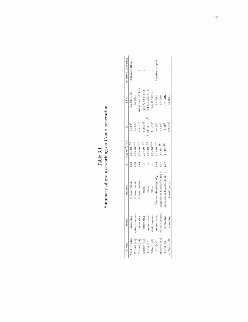
21

Tab

le3.

1Sum

mar

yof

grou

ps

wor

kin

gon

Com

bge

ner

atio

n

Gro

up

Shap

eM

ate

rial

nn2(c

m2/W

)Q

FSR

Inte

rtio

nL

oss

(dB

)

NIS

T-P

urd

ue

mic

rori

ng

Silic

on

nit

ride

1.9

82.5×

10−

15

3×

106

115-6

00

GH

z3

(lenced

fib

er)

Corn

ell

[48]

spir

al

reso

nato

rSilic

on

nit

ride

1.9

82.5×

10−

15

8×

105

20

GH

z–

Corn

ell

[38]

mic

rori

ng

Silic

on

nit

ride

1.9

82.5×

10−

15

1-5×

105

403

GH

z-1

.17

TH

z7

Razzari

[39]

mic

rori

ng

Silic

a1.7

2.3×

10−

16

1.2×

106

200

GH

z-6

TH

z9

MP

Q[3

7]

mic

roto

roid

Silic

a1.7

2.3×

10−

16

>108/2×

109

874

GH

z/86

GH

z–

Calt

ech

[49]

dis

kre

sonato

rSilic

a–

2.2×

10−

16

1.1×

108

2.6

-220

GH

z–

JP

L[4

1]

mic

roto

roid

Calc

ium

fluori

de(C

aF2)

1.4

43.2×

10−

16

6×

109

13

GH

z3

(pri

smcouple

)

OE

waves

[50]

obla

tesp

heri

od

magnesi

um

fluori

de(M

gF2)

1.3

71×

10−

16

3×

109

35

GH

z–

MP

Q[5

3]

cry

stallin

em

agnesi

um

fluori

de(M

gF2)

1.3

71×

10−

16

>109

107

GH

z–

NIS

T-C

O[5

2]

cry

stallin

efu

sed

quart

z–

–6.2×

108

36

GH

z–

22

In these resonators, the small confinement volume, high photon density, and long

photon storage time (proportional to the quality factor Q) induce a very strong light-

matter interaction. Their high optical finesse and small mode volume has led to

a significant reduction in the threshold of nonlinear optical processes. This leads

to generate a highly efficient FWM, where two pump photons are transformed into

two sideband photons through the Kerr nonlinearity. Provided that the pump is

powerful enough, an optical-frequency comb, sometimes referred to as a Kerr comb,

is generated through a cascaded FWM, resulting from interactions involving any four

photons fulfilling energy and angular momentum conservation requirements. Figure

3.1 can help to understand the mechanism. This mechanism is first proposed. But

recently a new approach is suggested which will be discussed in later. Here high Q

micro resonator (toroid) is pumped with intense CW source (> 10mW, 1550nm) [37].

The high n2 of the silica initiates the FWM process and results in the creation of signal

and idler photons from two pump photons: νpump+νpump = νI+νs as shown in Fig 3.1.

The conservation of energy ensures that the generated photon pairs are symmetric

in frequency with respect to the pump. This mechanism is resonantly enhanced by

the cavity if idler, signal and pump frequencies all coincide with optical modes of

the micro resonator. It is important to note that this process can be cascaded via

nondegenerate FWM among pump and first-order sideband, to produce higher order

sidebands (νpump + νI = νII + νs) as Fig. 3.1. This cascaded mechanism ensures

that the frequency difference of pump and first-order sidebands pump |νpump − νI | =

|νs − νII | is exactly transferred to all higher-order inter-sideband spacings. Thus,

provided that the cavity exhibits a sufficiently equidistant mode spacing, successive

FWM to higher orders intrinsically leads to the generation of sidebands with equal

spacing, that is, an optical frequency comb. But due to the dispersion in the cavity,

FSR varies with the optical frequency, so that the cavity resonances are not spaced

23

Fig. 3.1. Optical frequency comb generation in a micro resonator. (a)shows the resonator and the output comb spectrum. The individualcomb modes are spaced by FSR of the cavity. (b) shows the principleof the comb generation process. Degenerate and nondegenerate FWMallow conversion of a CW laser into an optical frequency comb [37].

24

Fig. 3.2. The role of dispersion in comb generation. Due to the dis-persion in the cavity, FSR varies with the optical frequency, so thatthe cavity resonances are not spaced equally in frequency. The gener-ated optical frequency comb (lines), in contrast, is perfectly equidis-tant [55].

equally in frequency. The generated optical frequency comb (lines), in contrast, is

perfectly equidistant as shown in Fig. 3.2. Therefore the generated sidebands walk

off from the cavity resonances with increasing sideband order, reducing the cavity

enhancement of the FWM. As a consequence, uncompensated cavity dispersion can

eventually limit the comb bandwidth.

3.3 On chip frequency comb characterization

Most investigations of Kerr combs have emphasized their spectral properties, in-

cluding optical and RF frequency stability. A few experiments have reported time

domain autocorrelation data [52, 55]. Here we expand the time domain understand-

ing of these devices by manipulating their temporal behavior through programmable

optical pulse shaping [8]. The large mode spacing of Kerr combs facilitates pulse

25

shaping at the individual line level, also termed optical arbitrary waveform generation

(OAWG) [6,13,56–58], a technology which offers significant opportunities for impact

both in technology (e.g., telecommunications, lidar) and ultrafast optical science (e.g.,

coherent control and spectroscopy). We demonstrate line-by-line pulse shaping of mi-

croresonators based frequency combs. An important feature of our approach is that

transform-limited pulses may in principle be realized for any spectral phase signature

arising from a coherent comb generation process. Furthermore, the ability to achieve

successful pulse compression provides new information on the passive stability of the

frequency dependent phase of coherent Kerr combs. Our time-domain experiments

also reveal differences in coherence properties associated with different pathways to

comb formation.

3.4 Si3N4 ring and Experiment setup

Fig. 3.3(a) shows a microscope image of a 40 µm radius silicon nitride microring

resonator with coupling waveguide (described in the Device fabrication section). For

robust and low-loss coupling of light into and out of the devices, a process for fiber

pigtailing the chip is developed at NIST by Dr. Houxun Miao, as shown in Fig.

3.3(b). The fiber pigtailing used for this device eliminates the time consuming task of

free space coupling and significantly enhances transportability. Other devices studied

employ a similar V-groove scheme to facilitate coupling alignment, but without per-

manent fiber attachment. Spectroscopy of the resonator’s optical modes is performed

with a swept wavelength tunable diode laser with time-averaged linewidth of less than

5 MHz. Figure 3.3(c) shows the transmission spectrum of two orders of transverse

magnetic (TM) modes (with different free spectral range (FSR) and coupling depth),

which have their electric field vectors predominantly normal to the plane of the res-

onator. Fig. 3.3(d) shows a zoomed in spectrum for a mode at ∼ 1556.43 nm with a

26

Fig. 3.3. (a) Microscope image of a 40 µm radius microring withthe coupling region. (b) Image of a fiber pigtail. (c) Transmissionspectrum of the microring resonator. (d) Zoomed in spectrum of anoptical mode with a 1.2 pm linewidth.

line width of 1.2 pm, corresponding to a loaded optical quality factor (Q) of 1.3×106.

The average FSR of the series of high Q modes is measured to be ∼ 4.8 nm. The

loaded Qs of the microresonators used in this chapter are typically 1×106 to 3×106.

Fig. 3.4 shows the experimental setup. CW light is launched into the microresonator,

with a polarization controller used to align the input polarization with the TM mode.

The generated frequency comb is launched to a line-by-line pulse shaper for spec-

tral phase measurement and correction, which are accomplished simultaneously by

optimizing the second harmonic generation (SHG) signal [4, 20], as described in Ex-

perimental procedure. The pulse shaper is also used to attenuate the pump line,

which in our experiments is typically 10 to 23 dB stronger than the adjacent comb

lines, and is sometimes programmed to attenuate some of the neighboring lines as

well. This results in a spectrum with line-to-line power variations reduced (but not

completely eliminated), which improves time domain pulse quality. In Ref. [20], the

27

Fig. 3.4. Scheme of the experimental setup for line-by-line pulseshaping of a frequency comb from a silicon nitride microring. CW:continuous-wave; EDFA: erbium doped fiber amplifier; FPC: fiberpolarization controller; µring: silicon nitride microring; OSA: opticalspectrum analyzer.

phase measurement by this SHG optimization method is compared with another in-

dependent method based on spectral shearing interferometry. The difference between

the two measurements was comparable to the π/12 step size of the SHG optimiza-

tion method. This provides an estimate of both the precision and the accuracy of our

phase measurement method. In addition to autocorrelation measurements which pro-

vide information on the temporal intensity, comb spectra are measured both directly

after the microresonator and after the pulse shaper and subsequent Erbium doped

fiber amplifier (EDFA).

3.5 Results

We have investigated comb generation with subsequent line-by-line shaping in a

number of devices and have observed two distinct paths to comb formation which

28

exhibit strikingly different time domain behaviors. Comb spectra measured directly

after generation are shown in Fig. 3.5, with estimated optical powers coupled to the

access waveguides given in the figure caption. In some cases the comb is observed to

form as a cascade of sidebands spaced by approximately one FSR that spread from the

pump (Figs. 3.5(a), 3.5(b) and 3.5(c) with comb spacings of ∼ 600 GHz, 230 GHz, 115

GHz, respectively). In such cases, which we will refer to as Type I comb formation,

high quality pulse compression is achieved, signifying good coherence properties. In

other cases (Figs. 3.5(d) and 3.5(f)), the initial sidebands are spaced by multiple

FSRs from the pump. With changes in pump power or wavelength, additional lines

spread out from each of these initial sidebands, eventually merging to form a spectrum

composed of lines separated by approximately one FSR. For example, Fig. 3.5(d)

shows a comb comprising nearly 300 lines spaced by 115 GHz; the initial sidebands,

which remain evident as strong peaks, are spaced by approximately 27 FSRs. Figure

3.6 shows another example of Type II comb formation. This route to comb formation,

which we will call Type II, has been discussed by several authors [39,41,59,60]. With

our devices, Type II formation results in a larger number of lines, but compressibility

is degraded in a way that provides clear evidence of partial coherence. Different

regimes of comb generation with distinct coherence properties have also recently been

reported for combs generated from silica microresonators [52]. In addition, comb

linewidth variations with different pumping conditions have also been reported [42].

Figure 3.7 shows a first set of pulse shaping results from a 40 µm radius mi-

croresonator (Fig. 3.3(a)) which generates the Type I comb shown in Fig. 3.5(a),

comprising twenty-six comb lines with a repetition rate of ∼ 600 GHz. The average

output power for an estimated 0.45 W coupled into the input waveguide is measured

to be 0.10 W. We select 9 comb lines (limited by the bandwidth of the pulse shaper

and the bandwidth of the EDFA before the autocorrelator) to perform the line-by-

29

Fig. 3.5. Spectra of generated optical frequency combs. For eachspectrum the CW pump wavelength, estimated power coupled to theaccess waveguide, and ring radius will be succinctly indicated (a)1543.07 nm, 0.45 W , 40 µm; (b) 1548.63 nm, 66 mW, 100 µm; (c)1547.15 nm, 1.4 W, 200 µm; (d) 1549.26 nm, 1.4 W, 200 µm; (e)1551.67 nm, 1.4 W, 100 µm; and (f) 1551.74 nm, 1.4 W, 100 µm.

30

Fig. 3.6. Spectra of generated optical frequency combs. CW pumpwavelengths are indicated in the figures. All the spectrums are takenfrom the same 200µm radius ring with 500 nm gap between ring andwaveguide. The CW power and other experimental parameters re-mains same (1.1 W).

31

line pulse shaping experiments. The spectrum after the pulse shaper and the spectral

phase profile which is found to maximize the SHG signal are shown in Fig. 3.7(a).

Fig. 3.7(b) shows the measured autocorrelation traces before and after spectral phase

correction. The signal appears nearly unmodulated in time without phase correction,

while a clear pulse-like signature is present after correction. Such pulse compression

clearly demonstrates successful line-by-line pulse shaping. The intensity profile of the

compressed pulse, calculated based on the spectrum (Fig. 3.7(a)) assuming a flat

spectral phase, has a full width at half maximum (FWHM) of 312 fs. The corre-

sponding intensity autocorrelation trace is calculated (as shown in Fig. 3.7(b)) and

is in good agreement with the experimental trace. The finite signal level remaining

between the autocorrelation peaks arises due to the finite number of lines and the

uneven profile of the spectrum. The widths of experimental and computed autocor-

relation traces are 460 fs and 427 fs, respectively, which differ by 7%. From this we

take the uncertainty in our 312 fs pulse duration estimation as 7%. As a preliminary

example of arbitrary waveform generation, we program the pulse shaper to apply a

π-step function to the spectrum of the compressed pulse; Fig. 3.7(c) shows the result.

The π step occurs at the pixel number 64 (corresponds to 1550 nm in wavelength).

Application of a π phase step onto half of the spectrum is known to split an original

pulse into an electric field waveform that is antisymmetric in time, sometimes termed

an odd pulse [27]. The resulting autocorrelation triplet is clearly visible as shown in

Fig. 3.7(c) and in good agreement with the autocorrelation that is computed based

on the spectrum in Fig. 3.7(a) and a spectral phase that is flat except for a π-step

centered at 1550 nm. This result constitutes a clear example of line-by-line pulse

shaping for simultaneous compression and waveform shaping. Similar high quality

pulse compression results have been achieved with other devices exhibiting Type I

comb formation. Figure 3.8 shows data for larger silicon nitride ring resonators (200

32

Fig. 3.7. (a) Spectrum of the generated comb (Fig. 3.5(a)) after thepulse shaper, along with the phase applied to the LCM pixels of thepulse shaper for optimum SHG. (b) Autocorrelation traces. Here thered line is the compressed pulse, the dark blue line is the uncom-pressed pulse, and the black line is calculated by taking the spectrumshown in Fig. 3.7(a) and assuming flat spectral phase. The contrastratio of the autocorrelation measured after phase compensation is 7:1.(c) The odd pulse: applied the same phase as Fig.3.7 (a), but withan additional π phase added for pixels 1-64 (wavelengths longer than1550 nm). Red line: experimental autocorrelation; black line: auto-correlation calculated using the spectrum of Fig. 3.7(a), with a π stepcentered at 1550 nm in the spectral phase. (d) Normalized intensityautocorrelation traces for compressed pulses, measured at 0, 14, and62 minutes after spectral phase characterization, respectively.

33

µm and 100 µm radii) which generate combs spaced by 115 GHz (Fig. 3(c)) and 230

GHz (Fig. 3(b)), respectively. These devices have fiber to fiber coupling loss as low as

3 dB when lensed fibers are used. The comb spectrum obtained for pumping the 200

µm radius device at ∼1547 nm exhibits 12 spectral lines, covering ∼10 nm bandwidth.

The comb spectrum obtained for pumping the 100 µm radius device at ∼ 1549 nm

exhibits 25 spectral lines, covering ∼ 45 nm bandwidth (20 spectral lines are left after

the shaper). The autocorrelation data again show that although originally the signals

are at most weakly modulated in time, phase correction results in obvious compression

into pulse-like waveforms, yielding autocorrelation FWHMs of 1.78 ps and 976 fs for

200 µm and 100 µm rings, respectively. In both cases the shape and on-off contrasts

of the autocorrelation are in fairly close agreement with the results simulated using

the measured spectra and assuming flat spectral phase. Time domain experiments

access information about coherence that is not available from frequency domain data

such as the comb spectra. For example, the ability to achieve pulse compression and

phase shaping results as shown in Figs. 3.7 and 3.8 provides clear evidence of coher-

ence across the comb spectrum. Note that intensity autocorrelation measurements

are insensitive both to overall optical phase and to optical phase that varies linearly

with frequency. Small changes in pulse repetition rate that would arise from small

changes in comb spacing would also be difficult to observe from autocorrelation data

(provided that the comb spacing remains uniform across the spectrum). However,

autocorrelations do provide information on changes in pulse duration associated with

spectral phase variations quadratic or higher in frequency. The close agreement in

the shape and on-off contrast of experimental autocorrelation traces, compared with

those calculated on the basis of the measured comb spectra (with flat spectral phase),

provides evidence that the obtained pulses are not only close to bandwidth-limited,

but also that they have high coherence. We also observe the autocorrelations over an

34

Fig. 3.8. (a) and (b) Spectra of the generated combs (correspondingto Fig. 3.5(c) and 3.5(b), respectively) after the pulse shaper, alongwith the phase applied to the LCM pixels for optimum SHG signals.(c) and (d) Autocorrelation traces corresponding to (a) and (b). Redlines are the compressed pulses after phase correction, dark blue linesare the uncompressed pulses, and black lines are calculated by tak-ing the spectra shown in (a) and (b) and assuming flat spectral phase.The contrast ratios of the autocorrelations measured after phase com-pensation are 14:1 and 12:1, respectively. Here Light gray traces showthe range of simulated autocorrelation traces.

35

extended period. Fig. 3.7(d) shows autocorrelation traces measured at different times

within a 62 minute interval, with the same spectral phase profile applied by the pulse

shaper for all measurements. Clearly the compression results remain similar over the

one hour time period indicated in the figure, which means that the relative average

phases of the comb lines must remain approximately fixed; slow drifts in relative av-

erage spectral phase must conservatively remain substantially below π. Assume now

that the field consists of lines at frequencies fo + nfrep + δfn, where fo is the carrier-

envelop offset frequency, frep is the repetition rate and the δfn refer to small fixed

shifts (assumed to be random and uncorrelated) of the individual frequencies from

their ideal, evenly spaced positions shown in Fig. 3.9. Such frequency shifts would

give rise to phase errors for the different spectral lines that grow in time according

to δφn = 2πδfnt. Since the δfn , and hence the linear drifts of the δφn, are taken as

uncorrelated, the characteristic size of the phase errors should (conservatively) satisfy

| δφn |< 0.7π in order to avoid significant waveform changes. With 3600 s observa-

tion time, we may then estimate that the assumed δfn are conservatively of the order

10−4 Hz or below. Our estimation is consistent with measurements performed for

combs from silica microtoroids, by beating with a self-referenced comb from a mode-

locked laser, which indicated uniformity in the comb spacing at least at the 10−3 Hz

level [37]. In contrast to the data presented so far for Type I combs, for which the

time domain data indicate good coherence, we now discuss our observations for Type

II combs, in which the initial sidebands are spaced by multiple FSRs from the pump.

First we discuss the compression experiments for a Type II comb obtained from a

200 µm radius ring pumped at ∼1549 nm, with the directly generated spectrum of

Fig. 3.5(d). We performed pulse compression experiments on a group of 24 comb

lines centered at ∼ 1558 nm. The spectrum after smoothing and phase correction

is shown in Fig. 3.11(a), and the autocorrelation data are shown in Fig. 3.11(d).

36

Fig. 3.9. Schematic diagram of frequency instability due to uncorre-lated line-to-line random phase. Here red arrow shows the effect ofδfn. δfn is the small fixed shifts (assumed to be random and uncor-related) of the individual frequencies from their ideal, evenly spacedpositions.

37

Fig. 3.10. Theoretical traces for nonlinear SHG autocorrelation mea-surements [18, 61]. The contrast ratio is 2:1 for continuous noise and2:1:0 for a finite duration noise burst. A single coherent pulse de-cays smoothly to zero background level. The pulse duration can beestimate from the full width half maximum (FWHM) ∆τ of the cor-relation trace G2(τ).

Once again phase compensation results in substantial compression compared to the

original waveform which shows only weak modulation. However, a new feature is that

the on-off contrast of the experimental autocorrelation is significantly worse than the

simulated trace which assumes phases that are frequency independent and constant

in time. The significantly degraded autocorrelation contrast is a hallmark of partial

coherence, which can occur when the spectral phase function varies in a nontrivial

way during the measurement time. It is known that the autocorrelation of continuous

intensity noise consists of a single peak centered at zero delay on top of a constant

positive background [18,61]. For a Gaussian random field with phases completely ran-

domized, the ratio of the peak value to the background is 2:1 as shown in Fig. 3.10.

The width of the autocorrelation peak gives the time scale for the intensity fluctua-

tions and does not imply the existence of a meaningful pulse duration. Furthermore,

the shape of the autocorrelation will not be affected by spectral phase shaping. On

the other hand, a coherent train of periodic pulses shows a series of peaks at delays

38

corresponding to the pulse separation and exhibits high autocorrelation contrast as

shown in Fig. 3.10. The autocorrelation trace does provide information on the pulse

duration and may definitely be changed by spectral phase shaping. In our experiments

with Type II combs, the autocorrelation shows contrast better than 2:1, but signifi-

cantly less than would be expected with perfect phase compensation. The portion of

the autocorrelation above the background remains responsive to spectral phase shap-

ing and allows compression to bandwidth-limited peaks which repeat at the inverse

of the comb spacing. This behavior corresponds to fluctuations of the spectral phase

on a time scale fast compared to the measurement time and with amplitude that is

significant but less than 2π, or in other words, partial coherence. In this regime the

signal consists of a deterministic average waveform superimposed with fluctuating

noise-like waveforms with the same repetition period. As explained in the Simulation

section, a rough estimate of the amplitude of the spectral phase fluctuations may be

obtained from the autocorrelation contrast. From the data in Fig. 3.14, we estimate

uncorrelated variations of the spectral phase over an approximate range of ±0.4π.

We have observed similar autocorrelation data characteristic of partial coherence in

a number of experiments with Type II combs, with minima of the experimental auto-

correlation traces lying above the simulated ones assuming full coherence by 17-28%

relative to the peak. The uncertainty in simulated traces is estimated by repeating

the simulations for 10-20 spectra recorded sequentially during the autocorrelation

measurement. The simulated traces with largest positive and negative variation in

contrast are shown as light gray lines in Fig. 3.11(d); this variation is significantly

less than that observed experimentally. In contrast, experimental autocorrelations for

Type I combs exhibit minima at most 5% above simulated traces. This difference is

sufficiently small that it may arise from a combination of effects such as uncertainty

or variation in power spectra used for simulations, imperfect compensation of average

39

spectral phase, and in some cases contributions from amplified spontaneous emission

(ASE). Although we cannot rule out some level of fast phase fluctuations, our Type

I combs clearly exhibit significantly lower phase fluctuations and higher coherence

than Type II combs. Fig. 3.11(e)-(f) shows another interesting example obtained

with 100 µm radius rings (for directly generated spectra, see Figs. 3.5(e)-(f)). Here

we pump a mode at ∼ 1551.67 nm, which most readily generates stable comb spectra

at 460 GHz spacing (twice the FSR). The spectrum after shaping and amplification

comprises eight lines as shown in Fig. 3.11(b), and the experimental and simulated

autocorrelation traces exhibit comparable contrast in Fig. 3.11(e). Thus, the coher-

ence of this comb appears to be high, similar to Type I combs. However, if the pump

wavelength is tuned sufficiently while maintaining lock [62] to the same resonance,

the spectrum broadens and intermediate comb lines fill in, resulting in a Type II

comb with 230 GHz spacing. Directly generated and post-shaper spectra and the

autocorrelation traces are shown in Figs. 3.5(f), 3.11(c) and 3.11(f) for pumping at ∼

1551.74 nm, a large shift compared to the low power linewidth. Although the shapes

of the compressed and simulated autocorrelation traces are similar, with a FWHM of

432 fs, the experimental background level is significantly increased, again indicating

reduced coherence for Type II combs. Figure 3.12 (c) also shows that odd pulse can

be found from TypeII combs also. Here we can easily see the triplet peaks but there

are mismatch between background. These examples demonstrate important coher-

ence differences in combs generated from the same resonance in the same device under

different pumping conditions.

3.6 Device fabrication

We have collaboration for device fabrication with NIST (National Institute of

Standard and Testing). Devices are fabricated by Dr. Houxun Miao at NIST. NIST

40

Fig. 3.11. (a), (b) and (c) Spectra of the generated comb (corre-sponding to Fig. 3.5(d), 3.5(e) and 3.5(f), respectively) after the pulseshaper, along with phase applied to the LCM pixels for optimum SHGsignals. (d), (e) and (f) Autocorrelation traces corresponding to (a),(b) and (c). Red lines are the compressed pulse after phase correction,dark blue lines are the uncompressed pulse, and black lines are thecalculated trace by taking the spectrum shown in (a), (b) and (c) andassuming flat spectral phase. Here Light gray traces show the rangeof simulated autocorrelation traces.

41

Fig. 3.12. (a) Spectrum of the generated comb (Fig. 3.5(f)) afterthe pulse shaper, along with the phase applied to the LCM pixelsof the pulse shaper for optimum SHG. (b) Autocorrelation traces.Here the red line is the compressed pulse, the dark blue line is theuncompressed pulse, and the black line is calculated by taking thespectrum shown in Fig. 3.12(a) and assuming flat spectral phase. (c)The odd pulse: applied the same phase as Fig. 3.12(a), but withan additional π phase added for wavelengths longer than 1554 nm.Red line: experimental autocorrelation; black line: autocorrelationcalculated using the spectrum of Fig. 3.12(a), with a π step centeredat 1555 nm in the spectral phase. Figs. 3.11(c)(f) are repeated asFigs. 3.12 (a)(b).

42

Fig. 3.13. (a)Si3N4 microring. (b)V groove (left rectangular shape)is connected to inverse tapered waveguide. (c)SEM of the wave guide(d) SEM of the V groove.

43

researchers start with a (100) silicon wafer. A 3 µm thick silicon dioxide layer was

grown in a thermal oxidation furnace. Then, a silicon nitride layer was deposited using

low-pressure chemical vapor deposition (LPCVD). The nitride layer was patterned

with electron-beam lithography and etched through using a reactive ion etch (RIE)

of CHF3/O2 to form microring resonators and waveguides coupling light into and

out of the resonators. The waveguides were linearly tapered down to a width of

∼ 100 nm at their end for low loss coupling to/from optical fibers [63]. Another

3 µm oxide layer was deposited using a low temperature oxide (LTO) furnace for

the top cladding. The wafer was annealed for 3 h at 12000C in an ambient N2

environment. A photolithography and liftoff process was used to define a metal mask

for V-grooves that provide self-aligned regions where the on-chip waveguide inverse

tapers are accessible by optical fibers placed in the V-grooves. After mask definition,

the V-grooves were formed by RIE of the unprotected oxide and nitride layers and

KOH etching of the silicon. Figure 3.13 shows the images and SEM of the device.

The height of the ring resonators is 430 nm and 550 nm for devices corresponding

to Figure 3.5, and Figure 3.5(b) to 3.5(f), respectively. The widths of the rings and

of the accessing waveguides are 2 µm and 1 µm throughout the paper. The radii

indicated within the paper are those at the outermost edge of the devices. The gap

between the ring and the waveguide is 700 nm in Fig 3(a), 500 nm in Fig 3.5(b), and

800 nm in Fig 3.5(c)-(f); the difference in ring-waveguide gap will modify the device

coupling.

3.7 Experimental procedure

Microresonators are pumped with CW powers estimated between 66 mW to 1.4 W

coupled into the input guide, in all cases well above the threshold for comb formation.

Line-by-line pulse shaping is implemented using a fiber-coupled Fourier-transform

44

pulse shaper that incorporates a 2×128 pixel liquid crystal modulator (LCM) array to

independently control both the intensity and phase of each spectral line. The output

waveform from the pulse shaper is fed to an intensity autocorrelation setup through

an EDFA. The path from the output of the microring chip to the autocorrelator

comprises ∼ 18 m of standard single mode fiber (SMF). The thickness of the BBO

crystal used for SHG is 0.6 mm, corresponding to an estimated 1-dB phase matching

bandwidth of 200 nm, well beyond the bandwidth of the combs investigated here.

Briefly, the phase is corrected by adjusting the phase of one comb line at a time to

maximize the SHG signal from the autocorrelation measurement at zero delay. To

optimize the SHG signal, the phase of the new frequency component is varied from 0

to 2π in steps of π/12. Once the SHG is optimized, the pulses are compressed close

to the bandwidth limit, and the opposite of the phase applied on the pulse shaper

gives an estimate of the original spectral phase after the comb has propagated to the

autocorrelator.

3.8 Simulation

Here, we briefly discuss the effect of variations of the phase of each of the comb lines

on the intensity autocorrelation. Simulations are performed by taking the spectrum

measured with an optical spectrum analyzer (OSA), assuming that the spectral phase

is flat, and then applying an uncorrelated random phase variation to each of the comb

lines. The intensity autocorrelation is then calculated. This is repeated for different

realizations of the phase variations, while keeping the same phase variation statistics.

Then the results are averaged to obtain the autocorrelation trace in the presence

45

of time varying spectral phases that are averaged in the experimental measurement

procedure. The temporal intensity Ii(t) for the ith realization is given by:

Ii(t) =|∑n

√pnexp

φniexpjn∆ωt |2 (3.3)

where pn is the power of the nth comb line, as obtained from the spectrum, ∆ω is the

comb spacing in angular frequency unit, and φni represents the random phase applied

to the nth comb line in the ith realization. The φni are uniformly distributed in the

range 0 to ∆φ and are mutually uncorrelated. The intensity autocorrelation for the

ith realization, G2i , is given by:

G2i(τ) =

∫Ii(t)Ii(t− τ)dt (3.4)

The G2i are not normalized since different realizations of intensity waveforms with

different peak to average power ratios will contribute differently to the autocorrelation

signals. The simulated autocorrelation is obtained by averaging N realizations as,

G2(τ) =

∑Ni=1G2i(τ)∑Ni=1G2i(0)

(3.5)

We show simulations based on the comb spectrum shown in Fig 3.11(c). The are

assumed to be uniformly distributed between 0 and a maximum phase variation ∆φ.

Simulations are performed for ∆φ = 0, 0.2π, 0.4π, 0.6π, 0.8π, and π. For each value of

∆φ, we average N=2000 realizations of the unnormalized autocorrelations. Fig. 3.14

shows the averaged autocorrelation traces. The backgrounds of the autocorrelation

traces clearly increase with increased ∆φ. However, the shape of the autocorrelation

is not very sensitive to ∆φ. The background level for ∆φ = 0.8π matches that of the

experimental autocorrelation trace of Fig. 3.11(f). Although this gives a rough esti-

mate of the amplitude of the phase fluctuations for the experiments of Figs. 3.11(c)

and 3.11(f), we note that this estimate is not necessarily precise since the form of the

phase fluctuation statistics is not known. For these simulations we postulated phase

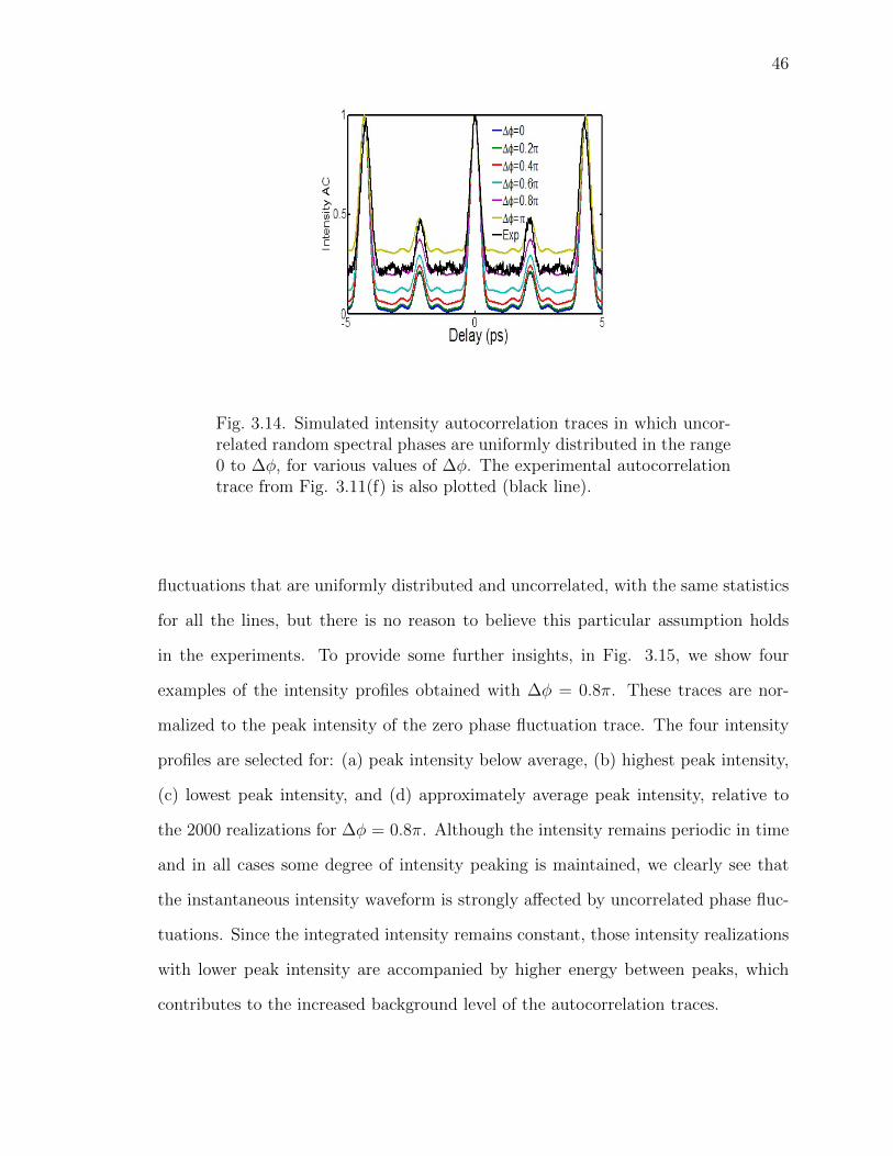
46

Fig. 3.14. Simulated intensity autocorrelation traces in which uncor-related random spectral phases are uniformly distributed in the range0 to ∆φ, for various values of ∆φ. The experimental autocorrelationtrace from Fig. 3.11(f) is also plotted (black line).

fluctuations that are uniformly distributed and uncorrelated, with the same statistics

for all the lines, but there is no reason to believe this particular assumption holds

in the experiments. To provide some further insights, in Fig. 3.15, we show four

examples of the intensity profiles obtained with ∆φ = 0.8π. These traces are nor-

malized to the peak intensity of the zero phase fluctuation trace. The four intensity

profiles are selected for: (a) peak intensity below average, (b) highest peak intensity,

(c) lowest peak intensity, and (d) approximately average peak intensity, relative to

the 2000 realizations for ∆φ = 0.8π. Although the intensity remains periodic in time

and in all cases some degree of intensity peaking is maintained, we clearly see that

the instantaneous intensity waveform is strongly affected by uncorrelated phase fluc-

tuations. Since the integrated intensity remains constant, those intensity realizations

with lower peak intensity are accompanied by higher energy between peaks, which

contributes to the increased background level of the autocorrelation traces.

47

Fig. 3.15. Selected simulated intensity profiles with uncorrelated ran-dom spectral phases that are uniformly distributed in the range 0 to∆φ = 0.8π. These plots are normalized to the peak intensity calcu-lated for the case of 0 phase fluctuations.

48

3.9 Conclusion

In summary, we have demonstrated line-by-line pulse shaping on frequency combs

generated from silicon nitride microring resonators. Combs formed via distinct routes

(Types I and II in the text) represent different time domain behaviors corresponding

to coherent and partially coherent properties. For Type I combs, nearly bandwidth-

limited optical pulses were achieved after spectral phase correction, and a simple ex-

ample of arbitrary waveform generation was presented. For type II combs, compressed

pulse trains were accompanied by significant autocorrelation background, signifying

larger spectral phase fluctuations. The ability to controllably compress and reshape

combs generated through nonlinear wave mixing in microresonators provides new ev-

idence of phase coherence (or partial coherence) across the spectrum. Furthermore,

in future investigations the ability to extract the phase of individual lines may furnish

clues into the physics of the comb generation process

49

4. TIME DOMAIN COHERENCE STUDY OF SILICON

NITRIDE MICRORESONATOR FREQUENCY COMBS

4.1 Introduction

The different types of comb formation are studied theoretically and experimen-

tally [47, 50–52]. However, the physics behind the comb generation is not yet fully

understood. In previous chapter, we studied the time domain properties of microres-

onator combs and revealed two different paths of comb formation that lead to strik-

ingly different time-domain behaviors [28]. Combs formed as a cascade of sidebands

spaced by a single free spectral range (FSR) that spread from the pump (which

were called Type I combs) exhibit high coherence. However, combs where the initial

sidebands are spaced by multiple FSRs that then fill in to give combs with single

FSR (which were called Type II combs) show partial coherence. As reported in this

work and also [28] autocorrelation data for combs exhibiting multi-FSR spacing show

good compressibility and high coherence. By slightly tuning the pump frequency, we

cause the missing lines to fill in to give a comb at single-FSR spacing - a Type II

comb. Now however the comb shows degraded compressibility and reduced coherence.

Apparently motivated by our findings in [28], the Kippenberg group has recently pub-

lished a paper in which they use RF beating measurements to characterize Type II

combs. Their data provide evidence that individual comb lines may exhibit spectral

substructure too fine to be resolved in normal OSA measurements, again consistent

with the simple picture of Type II comb formation. Here we study the properties of

Type II combs, by investigating the time domain behaviors of a few subfamilies of

0This work is published in [64]

50

frequency lines selected by a pulse shaper. We observe different coherence properties

for different groups of comb lines. Our recent time domain experiments result in

the new observation, not seen in the previous studies, that some sub families combs

exhibit markedly high coherence while whole family shows reduced coherence.

Figure 4.1 provides a schematic view of routes to comb generation. Figure 4.1(a)

depicts the Type I comb generation process, in which initial comb lines are generated

at ± 1FSR from the pump. Subsequent lines generated via cascaded four wave mixing

spread out from the center. Energy conservation ensures that the new lines are exactly

evenly spaced from the pump. Hence, this process is expected to result in a high

degree of coherence. Here and throughout this thesis, we use the term FSR to refer

to the average FSR for the series of high Q modes studied in the vicinity of the pump

frequency. It should be understood that the frequency difference between adjacent

modes, or FSR, varies slightly with frequency due to group velocity dispersion. Figure

4.1(b) shows the case where comb lines are initially generated at ±N FSRs from the

pump, where N is an integer greater than one (N=3 for the example shown). Such

behavior has been reported frequently in the literature. This process is again expected

to produce equal frequency spacings, which should result in high coherence. Our data

published in [28] demonstrate that both the process of Fig. 4.1(a) and the process of

Fig. 4.1(b) admit high quality pulse compression, providing evidence of stable spectral

phase and good coherence. By varying the pump laser, e.g., tuning it further into

resonance, additional spectral lines may be observed to fill in between those of Fig.

4.1(b), resulting in a Type II comb with nominally single FSR spacing. In the case

illustrated in Fig. 4.1(c), each of the lines from Fig. 4.1(b) has spawned additional

lines at ±1 FSR through an independent four-wave mixing process. Although the

lines within any one of the triplets resulting from this last process are expected to be

equally spaced, there is nothing to guarantee that such spacings are exact submultiples

51

of the original multiple-FSR comb spacing. In fact, due to group velocity dispersion,

it is very unlikely that all the new lines will be spaced precisely evenly in frequency. As

a result of such an imperfect frequency-division process, the relative phases between

certain groups of generated lines will vary with time. The time domain waveform,

which arises from the interference of the generated optical frequency components, will

therefore vary on a time scale set by the non uniformity of the frequency spacings.

In this sense we may say that the coherence is compromised.

One consequence of a process such as that illustrated in Fig. 4.1(c) would be that

different groups of lines may exhibit different degrees of coherence. For example, the

initial comb lines spaced by multiple FSRs, e.g., at frequencies {· · ·−6,−3, 0, 3, 6 · · · }

(relative to the pump in FSR units) in Fig. 4.1(b), are coupled and should therefore

have equal frequency spacing and high mutual coherence. Likewise, individual triplets

of lines, shown in Fig. 4.1(c), e.g., {−1, 0, 1}, which are spawned from a single line in

the previous step, are coupled and may also exhibit relatively high mutual coherence.

In our experiments we test this hypothesis by using a pulse shaper to select such

groups of lines out of a Type II comb. Time domain experiments confirm good

compressibility and coherence. In additional experiments a pulse shaper is used to

select other groups of lines for which direct coupling is not expected at the early stage

of comb formation depicted in Fig. 4.1. In such cases we observe that compressibility

and coherence are degraded. With further evolution beyond that sketched, the various

frequency triplets of Fig. 4.1(c) may each spawn additional lines through cascaded

four-wave mixing, which will then approximately overlap. However, because of the

imperfect frequency division, the overlap between newly generated lines will not be

exact. RF beating measurements have recently been used to characterize the evolution

of such Type II combs [47]. The beating data provide evidence that individual comb

lines may exhibit spectral substructure too fine to be resolved in normal optical

52

Fig. 4.1. Possible routes to comb formation. The optical frequencyaxis is portrayed in free spectral range (FSR) units. Arrows are drawnin an attempt to represent the approximate order in which new comblines are generated; no attempt is made to indicate all the couplingsinvolved in the four wave mixing process. (a) Case where initial comblines are spaced by one FSR from the pump line, with subsequentcomb lines, generated through cascaded four wave mixing, spreadingout from the center. (b) Case where initial comb lines are spacedfrom the pump line by N FSRs, where N>1 is an integer. Here N=3is assumed. (c) When the pump laser is tuned closer into resonance,additional lines are observed to fill in, resulting in spectral lines spacedby nominally 1 FSR.

53

spectrum analyzer measurements, consistent with the picture suggested here. Such

spectral substructure leads to increased noise if the now roughly, but not exactly,

overlapping frequency components fail to lock together. Increased RF noise in the

Type II regime was also reported in [52](L2 regime in their notation). In [52] further

tuning of the pump into the resonance led to a new regime (L3 in their notation)

characterized by substantial narrowing of the RF spectrum, with improved noise

performance. Reduction of the RF noise with further tuning into resonance was also

reported in [43, 47, 48]. The experiments presented in here focus on the Type II

regime and result in the new observation, not seen in previous studies, that some

subgroups of comb lines retain mutual coherence markedly higher than that of the

overall partially coherent Type II comb. Such coherence behavior contains structure

that bears on the early stages of the comb generation process.

4.2 Si3N4 ring and experimental setup

We use a silicon nitride ring resonator with 100 µm outer radius, 2 µm width and

550 nm thickness for the frequency comb generation. Light is coupled into/out of

the resonator via an on-chip waveguide with 1 µm width and 800 nm ring-waveguide

gap. The two ends of the waveguide are inversely tapered to 100 nm for low loss

waveguide-fiber coupling (1.5 dB per facet with lensed fiber). Our experiments use a

silicon nitride ring resonator with 100 µm outer radius, 2 µm waveguide width and

550 nm waveguide thickness for the frequency comb generation. The loaded Q of the

resonator is ∼3.2×105 and the normalized transmission at resonance is ∼ 20%. The

average FSR for the series of high Q modes is measured to be ∼1.85 nm (∼231 GHz

at 1550 nm center wavelength).

Strong CW pumping light (estimated to be 27.6 dBm into the accessing waveg-

uide) is launched into an optical mode at around 1551.6 nm. The generated frequency

54

comb is sent to a line-by-line pulse shaper, which both assists in spectral phase charac-

terization and enables pulse compression as shown in Fig. 3.4 [28]. By slowly tuning

the wavelength of the pump light from the blue to the red side, we first observed

an optical frequency comb with spectral lines spaced by 3 FSRs; then the spectral

lines in between fill in to form a comb with one FSR spacing. Figure 4.2 shows the

spectrum of the 3 FSR spacing comb after equalization by the pulse shaper. Figure

4.2b shows the autocorrelation traces before (blue) and after (red) phase correction

together with the calculated autocorrelation trace (black) for the spectrum shown

in Fig 4.2a assuming flat spectral phase. The measured autocorrelation trace after

phase correction is in good agreement with the calculation, indicating high coherence

of the comb. Fig 4.2c and 4.2d show the spectrum and the autocorrelation traces

of the corresponding 1 FSR comb (after slowly tuning the laser wavelength to the

red side). The significant difference of the measured autocorrelation trace from the

calculation indicates partial coherence for this Type II comb.

4.3 Results

To better understand the partial coherence properties of a Type II comb, we use

a pulse shaper to first filter out 3 subfamilies of comb lines from the spectrum shown

in Fig. 4.2c, with 3 FSR comb spacing each, while keeping the initial phase profile

the same as in the previous phase correction experiment shown in Fig. 4.2d. These

selected spectra and corresponding autocorrelation traces are shown in Fig 4.3. Fig.

4.3(a) shows the spectrum resulting when every third comb line is selected, including

the pump. This leaves lines {· · ·−6,−3, 0, 3, 6 · · · }, which is the same set of comb lines

present in the original multiple FSR spectrum of Fig. 4.2(a). The autocorrelation data

are similar to those of Fig. 4.2(b). Without phase compensation the autocorrelation is

modulated only weakly; phase compensation results in strong compression. As before,

55

Fig. 4.2. a) Spectrum of the generated 3 FSR spacing comb afterthe pulse shaper. (b) Autocorrelation traces corresponding to (a).(c) Spectrum of the generated 1 FSR spacing comb after the pulseshaper. Here we tune the CW laser 53 pm towards the red side thanthat of (a). (d) Autocorrelation traces corresponding to (c).

56

Fig. 4.3. Spectra and autocorrelation traces for 3 subfamilies of comblines with 3 FSR spacing selected from the spectrum shown in Fig.4.2(c). Blue and red traces are experimental traces before and af-ter phase compensation respectively. Black traces are calculated bytaking the OSA spectrums and assuming flat spectral phase.

an autocorrelation is also calculated for comparison by taking the measured spectrum

and assuming flat spectral phase. The very close agreement between experimental

and calculated autocorrelations, including on-off contrast, shows that high coherence

is maintained for this subfamily of lines.

Figures 4.3(c) and 4(d) show the results when a group consisting of every third

line is selected, but this time shifted from the pump. In particular, the pulse shaper

is programmed to pass lines {· · · − 5,−2, 1, 4 · · · } (frequencies relative to the pump

in FSR units). These lines are not directly coupled in the early stages of comb

formation outlined in Figs. 1(b)-(c). Figures 4.3(e) and (f) show the results of

another family with lines {· · · − 4,−1, 2, 5 · · · }. Now there is significant difference

57

between experimental and calculated (again assuming flat phase) autocorrelations.

For the data shown in Figs. 4.3(e-f), the spectrum is relatively smooth. Therefore the

autocorrelation calculated for full coherence and flat phase has high on-off contrast.

In this case the loss of contrast in the experiment is seen very prominently. Phase

compensation provides only weak compression, with the experimental autocorrelation

minimum falling only to ∼20 % of the peak in Fig. 4.3(f). Clearly, the coherence

is badly degraded. For the data of Figs. 4.3(c-d), the spectrum is uneven. As a

result the calculated autocorrelation for the case of full coherence already has high

background and low on-off contrast. Although additional loss of contrast is evident in

the experiment, indicating reduced coherence, the appearance is less dramatic. The

loss of mutual coherence for this set of lines will be supported with further data in

Fig. 4.6 below. Similar results are obtained in another experiment in which the pulse

shaper is programmed to pass every second line. Data obtained for the set of lines

including the pump{· · · − 6,−4,−2, 0, 2, 4 · · · } are shown in Figs. 4.4 (a) and (b);

similar data are shown in Figs. 4.4(c) and (d) are obtained for the complementary

set of alternating comb lines. Again poor autocorrelation contrast is observed, as

expected since a majority of the selected lines are not directly coupled in the early

stages of the presented model of comb formation.

4.4 Visibility curves

We further probe the coherence within the comb in experiments in which sets

comprising only three spectral lines are selected. For two spectral lines of fixed relative

power, the intensity autocorrelation is independent of the relative phase. Therefore,

three is the minimum number of lines which show sensitivity to spectral phase and

its variations. Following a procedure similar to that reported in [52], the pulse shaper

is used to vary the relative phase ∆φ of the longest wavelength line, with the phases

58

Fig. 4.4. Spectra and autocorrelation traces for 2 subfamilies of comblines with 2 FSR spacing selected from the spectrum shown in Fig.4.2(c). Blue and red traces are experimental traces before and af-ter phase compensation respectively. Black traces are calculated bytaking the OSA spectrums and assuming flat spectral phase.

59

Fig. 4.5. Autocorrelation traces for 3 line experiments for different ∆φfor lines {−3, 0, 3}, for which high coherence is observed. Here coloredlines are the experimental traces and black lines are the simulatedtraces.

of the other two lines arbitrarily set to zero. Figure 4.5 shows the evolution of the

autocorrelation traces with ∆φ when the pulse shaper selects lines {−3, 0, 3}. These

are a subset of the lines selected for the data of Figs. 4.3 (a) and (b) for which

high coherence was observed. The traces vary substantially as the relative phase is

changed, evolving from a single strong peak for ∆φ = 0 spaced by the autocorrelation

period T to a pair of weak peaks spaced by T/2 for ∆φ = π.

Here the autocorrelation period T ∼1.43 ps is the inverse of the ∼ 700 GHz

frequency separation between selected comb lines. When ∆φ is increased to 2π,

the autocorrelation recovers to the same form as ∆φ = 0. The experimental traces

(colored lines) are in close agreement with those calculated (black lines) based on the

measured spectrum and the programmed phases. The close correspondence between

60

Fig. 4.6. Autocorrelation traces for 3 line experiments for different ∆φfor lines {−2, 1, 4}, for which low coherence is observed. Here coloredlines are the experimental traces and black lines are the simulatedtraces.

the traces shows that the phase fluctuations are small and the coherence among

the selected lines is high. Quite different results are obtained for the triplet of lines

{−2, 1, 4}, which is selected from the set of lines of Fig. 4.3(c) which showed degraded

coherence. As shown in Fig. 4.6, the autocorrelation traces show only minor changes

as ∆φ is varied. This lack of dependence on the relative phase demonstrates that

the coherence among this triplet of lines, which are not directly coupled in the early

stages of our model of comb formation, is very weak. Similar results Fig. 4.7 showing

loss of coherence are observed when three lines are selected from the spectrum of Fig.

4.3(e).

61

Fig. 4.7. Autocorrelation traces for 3 line experiments for different∆φ for lines {−7,−4,−1}, for which low coherence is observed. Herecolored lines are the experimental traces and black lines are the sim-ulated traces.

62

Another way to view the results of such experiments is through the visibility curves

V (∆φ), as in [52]:

V (∆φ) =| p(τp)− p(τp + T/2) || p(τp) + p(τp + T/2) |

(4.1)

where p(τp) is the intensity autocorrelation peak, τp is the delay at which the peak

occurs. p(τp +T/2) is the value of the intensity autocorrelation half way between the

peaks. Note that because the autocorrelation is periodic for data sets such as those

of Figs. 4.5 and 4.6, we have three equivalent measurement points representing the

autocorrelation peaks [p(τp) and p(τp ± T )] and two equivalent measurement points

[p(τp ± T/2)] representing the autocorrelation value midway between the peaks. In

order to extract values for V from the data, for each autocorrelation trace we average

the equivalent points representing p(τp) and p(τp ± T/2), respectively, then plug into

the equation given above. We estimate the statistical uncertainty by evaluating V

using the various pairs of individual (not averaged) measurement points representing

the autocorrelation at and midway between its peaks. Another means to assess the

uncertainty is to compare the obtained values for V (0) and V (2π), since the visibil-

ity should be unchanged with 2π phase shift. For six of the seven visibility curves

reported below, the values for V (0) and V (2π) agree to within the estimated un-

certainty. Experimental visibility curves are compared with ideal theoretical curves

which are computed based on the measured optical power spectrum and assuming full

coherence. Multiple traces of the optical spectra are recorded simultaneously with

each autocorrelation measurement; this permits estimation of statistical uncertainty

in the scale of the theoretical curves due to small variations in the measured spectra.

Uncertainties quoted below represent one standard deviation.

Figure 4.8(a) shows visibility curves for triplets of lines separated by three FSRs.

The visibility of the {−3, 0, 3} triplet (red line), which includes the pump, exhibits

strong dependence on ∆φ, with minimum visibility equal to 8% ± 1% of the max-

63

Fig. 4.8. Visibility traces of (a) three subfamilies of 3 FSRs, (b) twosubfamilies of 2 FSRs, and (c) two subfamilies of 1 FSR. Here in thevisibility curves, red, green and black lines are the experimental data;blue lines are ideal theoretical curves calculated assuming full coher-ence based on the power spectra corresponding to the respective redline visibility curves. Numbers in curly braces indicate the 3 linesthat are used in the experiments. Error bars (shown for represen-tative curves) and shaded areas represent the mean ± one standarddeviation.

64

imum visibility. The data are close to the ideal theoretical curve (blue line). In

contrast, the visibility curves for triplets shifted away from the pump, {−2, 1, 4} and

{−7,−4,−1}, show only weak dependence on ∆φ, with minimum visibility equal to

66% ± 6% and 77% ± 7% of the maximum visibility, respectively. For comparison,

the ratio of minimum to maximum visibility that would be expected ideally (with

full coherence) are 9% ± 0.4% and 24% ± 1%, respectively. (The difference in ideal

visibility ratios is explained by differences in the relative intensities of the selected

lines.) The strong reduction in visibility clearly signifies degraded coherence. Figure

4.8(b) shows visibility curves for triplets {−4,−2, 0} and {−3,−1, 1}, each of which

is spaced nominally by 2 FSRs. Again only weak variation in visibility, hence low

coherence, is observed. These data consistently show low coherence for line triplets

which lack direct coupling in the early stages of our model of comb formation. Figure

4.8(c) shows visibility curves for triplets spaced nominally by a single FSR. For the

{−1, 0, 1} triplet, the visibility curve (red) exhibits large variation with ∆φ, with

minimum visibility equal to 13% ± 13% of the maximum visibility. This provides

evidence that relatively good coherence remains, consistent with the coupling within

this triplet of lines suggested by our model, Fig. 4.1(c). As a counter example, we

next selected the triplet {−2,−1, 0}, comprising the pump and two lines to one side

of the pump. Since the -2 line would not have direct coupling to the -1 and 0 lines

in the second step of our hypothesized comb generation model, degraded coherence

is predicted. This is confirmed by the corresponding (black) visibility curve in Fig.

4.8(c), for which the variation is significantly reduced with minimum visibility equal

to 58%± 5% of the maximum visibility.

Our data give qualitative support to the simple model suggested by Fig. 4.1(c),

namely, groups of lines that are directly coupled should have high coherence, while

groups of lines that are not directly coupled should lack coherence. However, at a

65

quantitative level, the correspondence is not complete. For example, the peak visibil-

ity data for the {−1, 0, 1} triplet in Fig. 4.8(c) is somewhat lower than the theoretical

trace, which suggests the coherence may be less than 100 %. Similarly, although vari-

ation of the visibility for the {−2,−1, 0} triplet in Fig. 4.8(c) is clearly suppressed

compared to the {−1, 0, 1} case, the suppression is incomplete: some variation re-

mains. This suggests that although the coherence is reduced, it does not reach zero.

An explanation for these observations may involve further cascaded four-wave mixing

beyond the early stage of comb formation portrayed in Fig. 4.1(c), which will cause

the individual subcombs to spread until they overlap, as discussed in [47] for both

crystalline magnesium fluoride and planar silicon nitride microresonators. Figure 4.9

shows a sketch illustrating this process, in this case with the initial lines separated by

6 FSRs. The important point is that in the final stage illustrated, any region of the

comb spectrum consists of distinct overlapped subcombs (distinct in the sense that

either the offset frequencies, the line spacings, or both are different). Because the

pulse shaper does not resolve the distinct subcombs, the overall coherence of selected

comb lines depends on the simultaneous contributions of different subcombs. Simu-

lations that model the generated frequencies as coherent within individual subcombs

but incoherent across distinct subcombs are able to approximately reproduce our ob-

servations in the visibility data, provided that the number of lines in the subcombs

and their relative intensities are appropriately adjusted.

As a final point, we comment on the relationship between our experiments and

those presented in [47]. Our measurements provide information mainly on which

sets of lines stay in phase with each other and which do not. They do not directly

tell us whether phase variations (when significant) arise because different subsets of

lines have different offset frequencies, because different subsets of lines have differ-

ent repetition frequencies, or because of other unspecified reasons. In this sense we

66

Fig. 4.9. Proposed model for type II comb formation. (a) First:generation of a cascade of sidebands spaced by N FSRs (Nδω) fromthe pump. Here N=6 is illustrated. (b)-(c) The 2nd event is anindependent four-wave mixing process, which creates new sidebandsspaced by a different amount,±nδω′(n=1,2 or 3....for different lines),from each of the lines in the previous step. Due to dispersion, it is veryunlikely that the new frequency spacings will be exact submultiplesof the original N FSR spacing; i.e.,δω

′ 6= δω.

67

get different information than [47], which beats the comb generated by the microres-

onator with a self-referenced comb from a mode-locked laser to precisely measure the

individual optical frequencies. On the other hand, our measurements directly probe

optical coherence, which the measurements in [47] do not access.

4.5 Conclusion

In conclusion, we have used an optical pulse shaper to probe the coherence of

a frequency comb generated via cascaded four-wave mixing in a silicon nitride mi-

croresonator. Our measurements reveal a striking variation in the degree of mutual

coherence exhibited for different groups of lines selected out of the full comb. The

structure observed in the mutual coherence provides evidence consistent with a simple

model of partially coherent comb formation.

68

5. FUTURE WORK

5.1 Intoduction

In this chapter, several experiments which are very interesting and will give us

more insight about comb formations are discussed. We discussed current limitation

and also ways to solve the limitations.

5.2 Future work

5.2.1 SHG Frequency-resolved optical gating

In Kerr combs, some of the lines have very low power. We need to find an mea-

surement technique which can detect phases from very low power. The technique

discussed in chapter 2 can be used. As an second measurement technique, we are

planning to use SHG frequency-resolved optical gating (FROG). By using aperiodi-

cally poled lithium niobate (A-PPLN) waveguides as the nonlinear medium, our group

demonstrated ultra low-power multishot SHG FROG in the telecommunication band

with a measurement sensitivity of 2.0×10−6mW 2, an 8 orders of magnitude improve-

ment over SHG FROG using bulk crystals and 5 orders of magnitude better than

previously reported for any FROG measurement modality [65]. Here we will use a

fiber-pigtailed A-PPLN waveguide with ∼50 nm phase-matching curve centered at

1542 nm at room temperature. This will cover the combs spectrum after the pulse

shaper and EDFA. Figure 5.1 shows the scheme of the polarization insensitive FROG

setup [65]. The polarization of the signal pulse from comb is scrambled with a wide

band fiber pigtailed polarization scrambler (General Photonics Corporation, PCD-

69

Fig. 5.1. Polarization insensitive ultra low-power SHG FROG setup [65].

104), with more than 100 nm operating range centered at 1550 nm, and 700 KHz

scrambling frequency. The scrambled pulses are then launched into a Michelson in-

terferometer to produce pulse pairs with various delays. One of the interferometer

arms is dithered over a few optical cycles at a rate of 160 Hz to wash out the in-

terference fringes. The pulse pairs are coupled into the A-PPLN waveguide with a

fiber-pigtailed collimator to produce SHG signals. The SHG spectrum for each delay

is recorded by a spectrometer and an intensified CCD camera which yields the raw

FROG data. To get a background-free FROG trace, a spectrum taken at a large delay

is subtracted from the raw data. The spectrum of the pulses is recorded separately by

an OSA for frequency marginal correction. We use commercial software (Femtosoft

FROG) to completely retrieve the intensity and phase information of the pulses.

70

5.2.2 Comb improvement and dispersion measurement

We have the micro resonator from NIST which has 10 times higher quality factor

than that of Cornell micro resonator as seen in table 3.1. But we have narrower

bandwidth than that of them. The reason may be due to the dispersion of the

waveguide as discussed in section 4.2. We have done some simulation with the device

dimensions for waveguide dispersion. The simulation is done in MPB [66]. The

schematic model of device is shown in Fig 5.2. We have used fixed n equal to 1.42 and

2.05 for SiO2 and Si3N4 respectively unless otherwise stated. Here the cladding region

is SiO2 around ∼ 3µm. We have seen that the dispersion is quite high for the device as

shown in Fig 5.3. Here we have varied n also as we guess n to be 2.05 but it may varies

on fabrication process. As n is depend on fabrication process, we need to calculate

dispersion experimentally. Also in the simulation, we assumed the material dispersion

to be zero. But that may be not true. To verify both of these we are planning to do

dispersion experiment. For dispersion calculation, we ( also one colleague Jian Wang

from Prof. Qi) will use optical parametric oscillator (OPO) which has wavelength

coverage from 1.1 to 2.6 µm. It has 150 mW power. We will use Fourier-transform

spectral interferometry (FTSI) [67]. Schematic diagram of the experimental setup is

shown in Fig 5.4. A 130 femtosecond laser pulse train from a tunable OPO is split such

that one part is sent to the waveguide and the other travels through a reference arm.

The polarization is optimized to excite the low-loss TE-like mode of the waveguide.

Output of the waveguide is combined with the reference arm in a coupler. When

the output pulses are measured with an OSA one observes a wavelength-dependent

modulation of the optical spectrum, or a spectral interferogram. The frequency of the

modulation of the spectral interferogram is proportional to the time delay between

the two pulses. By extracting the variation of the time delay as a function of the

center wavelength of the pulses, one obtains the group index of refraction of the entire

71

Fig. 5.2. The model used for simulation. Here h,b and w are theheight, base of the Si3N4 and cladding layer(SiO2) dimension respec-tively.

72

Fig. 5.3. Simulation results of the present device. Here h,b and θare the height, base and angle from the vertical direction of the Si3N4

respectively.

73

Fig. 5.4. Schematic diagram of the experimental setup for dispersioncalculation. Here OPO: optical parametric osillator; DUT: deviceunder test.

system. In order to find the group index solely of the waveguides, the measurements

are repeated with the waveguide removed from the system. For now, we also try to

calculate optimum device performance by simulation. From, Fig 5.5, we see that if

we have device with θ=2.5 or 3 and b=1.5 or 2µm, then h=500-550 nm will be good

choice as in that region dispersion will be zero. Our 2nd generation devices have these

dimensions.

5.3 RF beating experiment

Clearly there is much more left to be investigated about TypeII comb formation.

Different lines may act differently. We believe such investigations will enhance our

understanding of comb formation, hopefully providing insight that will aid efforts to

enforce coherence. Frequency domain studies will include measurement of RF spectra

obtained by beating comb lines with reference lasers, including a commercial, self-

referenced, mode-locked fiber laser comb that we have recently ordered. Schematic

diagram of this experiment is shown in Fig. 5.6(a). Different sideband orders gener-

ated from adjacent comb lines can overlap, again leading to RF beat signals as shown

in Fig 5.6(b) diagnostic of comb uniformity and noise.

74

Fig. 5.5. Simulation results with various dimensions to find optimumdevice dimension for next generation device. Here h,b and θ are theheight, base and angle from the vertical direction of the Si3N4 respec-tively.

75

Fig. 5.6. (a) Schematic diagram for RF beating experiment. (b)expected results: One line will be beat with tunable laser and multiplelines will be seen in RF spectrum analyzer.

76

5.4 Pulse generation from Kerr combs

Recently we have observed that with sufficient care, at least partially reproducible

spectral phase profiles may be observed in successive lab sessions with the pump laser

turned off in between as shown in Figs 5.7 and 5.8. Fig. 5.7 shows the spectrum after

equalization by the pulse shaper, the applied spectral phase, and the corresponding

autocorrelation (AC) traces. Here we first get comb with 3 FSRs spacing with high

coherent temporal behavior. In Fig 5.7(b) red line is the AC trace when we apply red

dot phases of Fig 5.7(a). Black line is the calculated AC considering spectrum shown

in Fig 5.7(a) and assuming spectrum flat spectral phases. Blue line is the AC trace

without pulse compression. Green line is the experimental AC trace when we apply

green dot phases of Fig 5.7(a). Here we did the phase compensation 24 hrs ago with

green dot phases. Then we turn off the laser. On next day, we turn on laser and with

almost same conditions of the previous day, we generate the comb. Then redo the

pulse compression experiment and get red line curve. Then applying the previous day

phase file we also get pulse compression. Both of them matches well with calculated

AC traces and also shows clear pulse compression. Fig 5.8 shows the spectrum for

the same devices. After tuning a CW wavelength we get 1 FSR spacing comb from 3

FSRs comb like Fig 5.7 with partial coherent temporal behavior. We normally called

this as Type II comb. Here the color sequences as those of Fig 5.7 . The red and

green traces matches well with each other but show difference with the calculated

trace. Further researches are needed to know whether pulses produced within the

microresonators themselves. Also why two different phase profile have almost same

pulse shape as shown in Figs 5.7 and 5.8.

77

Fig. 5.7. High coherent temporal case: (a) Spectrum of the generatedcomb after the pulse shaper with applied phases. (b) Autocorrelationtraces. Here red line is the experimental AC trace when we applyred dot phases of Fig 5.7(a). Black line is the calculated AC con-sidering spectrum shown in Fig 5.7(a) and assuming spectrum flatspectral phases. Blue line is the experimental AC trace without pulsecompression. Green line is the experimental AC trace when we applygreen dot phases of Fig 5.7(a).

78

Fig. 5.8. Partial coherent temporal case: (a) Spectrum of the gener-ated comb after the pulse shaper with applied phases. (b) Autocor-relation traces. Here red line is the experimental AC trace when weapply red dot phases of Fig 5.8(a). Black line is the calculated ACconsidering spectrum shown in Fig 5.8(a) and assuming spectrum flatspectral phases. Blue line is the experimental AC trace without pulsecompression. Green line is the experimental AC trace when we applygreen dot phases of Fig 5.8(a).

79

5.5 On-chip pulsed light source

In my current research, I used free space pulse shaper. But if we can make on-

chip OAWG, we also can have pulse shaper on chip. So combing Kerr comb chips

and pulse shaper chip will be a breakthrough. An integrated 8-channel optical spec-

tral shaper is demonstrated by cascading eight silicon microring add-drop filters on

a silicon-on-insulator platform [68, 69]. Each microring is side coupled to a Mach-

Zehnder arm, which is embedded in the through port waveguide. Compact metal

heaters are fabricated on top of the microrings and the Mach-Zehnder arms for ther-

mal control purpose. Thermal tuning changes the resonance wavelength and power

spectrum extinction ratio of each microring add-drop filter. It consequently controls

the spectral shaper in a programmable fashion. RF waveforms are demonstrated

with fundamental frequencies from 10 GHz to 60 GHz. Various types of RF signals,

including single frequency waveform, 1800 phase shift RF burst, apodized single fre-

quency waveform and chirped burst, have been generated through this chip. Their

demonstration may be a starting point for the miniaturization of ultra broad band-

width microwave photonics and for system-level application of silicon photonics. In

the setup introduced above, single mode fiber spool as the stretcher source is required

to provide dispersion. This part is hard to be deployed on chip. An advanced design

for RFAWG using tunable delay line is investigated [69]. Here an optical pulse is

separated into eight pulses by cascaded add-drop microring resonators. Each pulse

is delayed by an all-pass microring train. Then eight pulses are recombined together

to form the arbitrary waveform. The on-chip pulse pulsed light source will be as Fig

5.9:

80

Fig. 5.9. Schematic diagram for on-chip pulsed light source.

LIST OF REFERENCES

81

LIST OF REFERENCES

[1] T. Udem, R. Holzwarth, and T. W. Hansch, “Optical frequency metrology,”Nature, vol. 416, pp. 233–237, 2002.

[2] D. J. Jones, S. A. Diddams, J. K. Ranka, A. Stentz, R. S. Windeler, J. L. Hall,and S. T.Cundiff, “Carrier-envelope phase control of femtosecond mode-lockedlasers and direct optical frequency synthesis,” Science, vol. 288, pp. 635–639,2000.

[3] C. B. Huang, “Control and characterization of phase-modulated continious-wavelaser frequency combs,” Thesis, 2008.

[4] C.-B. Huang, S. Park, D. E. Leaird, and A. M. Weiner, “Nonlinearly broad-ened phase-modulated continuous-wave laser frequency combs characterized us-ing dpsk decoding,” Opt. Express, vol. 16, no. 4, pp. 2520–2527, 2008.

[5] R. Wu, V. R. Supradeepa, C. M. Long, D. E. Leaird, and A. M. Weiner, “Gen-eration of very flat optical frequency combs from continuous-wave lasers usingcascaded intensity and phase modulators driven by tailored radio frequency wave-forms,” Opt. Lett., vol. 35, no. 35, pp. 3234–3236, 2010.

[6] Z. Jiang, D. E-Leaird, , and A. M. Weiner, “Optical arbitrary waveform gen-eration and characterization using spectral line-by-line control,” J. LightwaveTechnol, vol. 24, no. 7, pp. 2487–2494., 2006.

[7] V. R. Supradeepa, D. E. Leaird, and A. M. Weiner, “Single shot amplitude andphase characterization of optical arbitary waveformsl,” Opt. Express, vol. 17,pp. 14434–14443, 2009.

[8] A. M. Weiner, “Femtosecond pulse shaping using spatial light modulators,” Re-view of Scientific Instruments, vol. 71, no. 5, pp. 1929–1960, 2000.

[9] http: //en.wikipedia.org/wiki/File:Optical-fibre.svg.

[10] F. Ferdous, D. E. Leaird, C. B. Huang, and A. M. Weiner, “Dual comb electricfield cross-correlation technique for optical arbitrary waveform characterization,”Optics Letters, vol. 34, pp. 3875–3877, 2009.

[11] T. Udem, R. H. Holzwarth, and T. W. Hansch, “Optical frequency metrology,”Nature, vol. 416, no. 5, pp. 233–237, 2002.

[12] D. J. Jones, S. A. Diddams, J. K. Ranka, A. Stentz, R. S. Windeler, J. L.Hall, and S. Cundiff, “Carrier-envelope phase control of femtosecond mode-locked lasers and direct optical frequency synthesis,” Science, vol. 288, no. 5466,pp. 635–639, 2000.

82

[13] Z. Jiang, D. S. Seo, D. E. Leaird, and A. M. Weiner, “Spectral line by line pulseshaping,” Opt. Lett., vol. 30, pp. 1557–1559, 2005.

[14] Z. Jiang, C.-B. Huang, D. E. Leaird, and A. M. Weiner, “Optical arbitrarywaveform processing of more than 100 spectral comb lines,” Nature Photonics,vol. 1, pp. 463 – 467, 2007.

[15] R. P. Scott, N. K. Fontaine, J. Cao, K. Okamoto, B. H. Kolner, J. P. Heritage,and S. J. B. Yoo, “High-fidelity line-by-line optical waveform generation andcomplete characterization using frog,” Opt. Express, vol. 15, no. 16, pp. 9977–9988, 2007.

[16] D. J. Kane and R. Trebino, “Characterization of arbitrary femtosecond pulsesusing frequency-resolved optical gating,” IEEE J. Quantum Electron, vol. 29,no. 2, pp. 571–579, 1993.

[17] C. Iaconis and I. Walmsley, “Spectral phase interferometry for direct electric-fieldreconstruction of ultrashort optical pulses,” Opt. Lett., vol. 23, no. 10, pp. 792–794, 1998.

[18] A. M. Weiner, Ultrafast optics. Wiley, 2009.

[19] V. R. Supradeepa, D. E. Leaird, and A. M. Weiner, “Optical arbitrary wave-form characterization via dual-quadrature spectral interferometry,” Opt. Express,vol. 17, no. 1, pp. 25–33, 2009.

[20] H. Miao, D. E. Leaird, C. Langrock, M. M. Fejer, and A. M. Weiner, “Opticalarbitrary waveform characterization viadual-quadrature spectral shearinginter-ferometry,” Opt. Express, vol. 17, no. 5, pp. 3381–3389, 2009.

[21] I. Coddington, W. C. Swann, and N. R. Newbury, “Coherent multiheterodynespectroscopy using stabilized optical frequency combs,” Phys. Rev. Lett., vol. 100,no. 1, p. 013902, 2008.

[22] C. Dorrer, D. C. Kilper, H. R. Stuart, G. Raybon, and M. G. Raymer, “Linearoptical sampling,” IEEE Photon. Technol. Lett., vol. 15, no. 12, pp. 1746–1748,2003.

[23] I. Coddington, W. C. Swann, and N. R. Newbury, “Coherent linear optical sam-pling at 15 bits of resolution,” Opt. Lett., vol. 34, no. 14, pp. 2153–2155, 2009.

[24] H. Murata, A. Morimoto, T. Kobayashi, and S. Yamamoto, “Optical pulse gen-eration by electro optic modulation method and its application to integratedultrashort pulse generators,” IEEE J. Sel. Top. Quantum Electron., vol. 6, no. 6,pp. 1325–1331, 2000.

[25] T. Sakamoto, T. Kawanishi, and M. Izutsu, “Asymptotic formalism for ultraflatoptical frequency comb generation using a mach-zehnder modulator,” Opt. Lett.,vol. 32, no. 11, pp. 1515–1517, 2007.

[26] K. Naganuma, K. Mogi, and H. Yamada, “Group-delay measurement usingthe fourier transform of an interferometric cross correlation generated by whitelight,” Opt. Lett., vol. 15, no. 7, pp. 393–395, 1990.

83

[27] J. Heritage, A. m. Weiner, and R. N. Thurston, “Picosecond pulse shaping byspectral phase and amplitude manipulation,” Opt. Lett., vol. 10, pp. 609–611,1985.

[28] F. Ferdous, H. Miao, D. Leaird, K. Srinivasan, J. Wang, L. Chen, L. Varghese,and A. Weiner, “Spectral line-by-line pulse shaping of on-chip microresonatorfrequency combs,” Nature Photonics, vol. 5, pp. 770–776, 2011.

[29] S. A. Diddams, J. C. Bergquist, S. R. Jefferts, and C. Oates, “Standards of timeand frequency at the outset of the 21st century,” Science, vol. 306, pp. 1318–1324,2004.

[30] F. Keilmann, C. Gohle, and R. Holzwarth, “Standards of time and frequency atthe outset of the 21st century,” Opt. Lett., vol. 29, pp. 1542–1544, 2004.

[31] A. Schliesser, M. Brehm, F. Keilmann, and D. van der Weide, “Frequency-combinfrared spectrometer for rapid and remote chemical sensing,” Opt. Express,vol. 13, pp. 9029–9038, 2005.

[32] S. Diddams, L. Hollberg, and V. Mbele, “Molecular fingerprinting with the re-solved modes of a femtosecond laser frequency comb,” Nature, vol. 445, pp. 627–630, 2007.

[33] M. Thorpe, K. Moll, J. Jones, B. Safdi, and J. Ye, “Broadband cavity ring-down spectroscopy for sensitive and rapid molecular detection,” Nature, vol. 311,pp. 1595–1599, 2006.

[34] T. Yamamoto, T. Komukai, K. Suzuki, and A. Takada, “Spectrally flattenedphase-locked multi-carrier light generator with phase modulators and chirpedfibre bragg grating,” Electron. Lett., vol. 43, pp. 1040–1042, 2007.

[35] M. Kourogi, K. Nakagawa, and M. Ohtsu, “Wide-span optical frequency combgenerator for accurate optical frequency difference measurement,” IEEE J.Quantum Electron., vol. 29, pp. 2693–2701, 1993.

[36] T. Kippenberg, R. Holzwarth, and S. Diddams, “Microresonator-based opticalfrequency combs,” Science, vol. 332, pp. 555–559, 2011.

[37] P. DelHaye, A. Schliesser, O. Arcizet, T. Wilken, R. Holzwarth, and T. J. Kip-penberg, “Optical frequency comb generation from a monolithic microresonator,”Nature, vol. 450, pp. 1214–1217, 2007.

[38] J. S. Levy, A. Gondarenko, M. A. Foster, A. C. Turner-Foster, A. L. Gaeta, andM. Lipson, “Cmos-compatible multiple-waelength oscillator for on-chip opticalinterconnects,” Nature Photonics, vol. 4, pp. 37–40, 2010.

[39] L. Razzari, D. Duchesne, M. Ferrera, R. Morandotti, S. Chu, B. E. Little, andD. J. Moss, “Cmos compatible integrated optical hyper-parametric oscillator,”Nature Photonics, vol. 4, pp. 41–45, 2010.

[40] P. DelHaye, O. Arcizet, A. Schliesser, R. Holzwarth, and T. J. Kippenberg, “Fullstabilization of a microresonator-based optical frequency comb,” Phy. Rev. Lett.,vol. 101, no. 5, pp. 053903–1–053903–1, 2008.

84

[41] I. S. Grudinin, N. Yu, and L. Maleki, “Generation of optical frequency combswith a CaF2 resonator,” Opt. Lett., vol. 34, no. 7, pp. 878–880, 2009.

[42] P. Del’Haye, T. Herr, E. Gavartin, M. L. Gorodetsky, R. Holzwarth, and T. Kip-penberg, “Octave spanning tunable frequency comb from a microresonator,” Phy.Rev. Lett., vol. 107, p. 063901, 2011.

[43] M. A. Foster, J. S. Levy, O. Kuzucu, K. Saha, M. Lipson, , and A. L. Gaeta,“Silicon-based monolithic optical frequency comb source,” Opt. Express, vol. 19,pp. 14233–14239, 2011.

[44] Y. Okawachi, K. Saha, J. S. Levy, Y. H. Wen, M. Lipson, and A. L. Gaeta,“Octave-spanning frequency comb generation in a silicon nitride chip,” Opt. Lett.,vol. 36, pp. 3398–3400, 2011.

[45] M. Ferrera, D. Duchesne, L. Razzari, M. Peccianti, R. Morandotti, P. Cheben,S. Janz, D.-X. Xu, B. E. Little, S. Chu, and D. J. Moss, “Low power four wavemixing in an integrated and micro-ring resonator with q = 1.2 million,” OpticsExpress, vol. 17, pp. 14098–14103, 2009.

[46] I. H. Agha, Y. Okawachi, M. A. Foster, J. E. Sharping, and A. L. Gaeta, “Four-wave-mixing parametric oscillations in dispersion-compensated high-q optical mi-crospheres,” Phys. Rev. A, vol. 76, p. 043837, 2007.

[47] T. Herr, J. Riemensberger, C. Wang, K. Hartinger, E. Gavartin, R. Holzwarth,M. L. Gorodetsky, , and T. J. Kippenberg, “Universal dynamics and noise ofkerr frequency comb formation in microresonators,” Nature Photonics, vol. 6,pp. 480–487, 2012.

[48] A. R. Johnson, Y. Okawachi, J. S. Levy, J. Cardenas, K. Saha, M. Lipson, andA. L. Gaeta, “Chip-based frequency combs with sub-100-ghz repetition rates,”Optics Letters, vol. 37, pp. 875–877, 2012.

[49] J. Li, H. Lee, T. Chen, and K. J. Vahala, “Low-pump-power, low-phase-noiseand microwave to millimeter-wave repetition rate operation in microcombs,” http://arxiv.org/pdf/1208.5256.pdf.

[50] W. Liang, A. A. Savchenkov, A. B. Matsko, V. S. Ilchenko, D. Seidel, andL. Maleki, “Generation of near-infrared frequency combs from a mgf2 whisperinggallery mode resonator,” Opt. Lett., vol. 36, p. 2290, 2011.

[51] A. A. Savchenkov, A. B. Matsko, W. Liang, V. S. Ilchenko, D. Seidel, andL. Maleki, “Transient regime of kerr frequency comb formation,” Phys. Rev.A., vol. 86, p. 013838, 2012.

[52] S. B. Papp and S. A. Diddams, “Spectral and temporal characterization ofa fused-quartz microresonator optical frequency comb,” Phy. Rev. A, vol. 84,p. 053833, 2011.

[53] C. Y. Wang, T. Herr, P. Del’Haye, A. Schliesser, J. Hofer, R. Holzwarth, T. W.Hnsch, N. Picqu, and T. J. Kippenberg, “Mid-infrared optical frequency combsbased on crystalline microresonators,” http: //arxiv.org/pdf/1109.2716v1.pdf.

[54] P. Barclay, K. Srinivasan, and O. Painter, “Nonlinear response of silicon photoniccrystal microresonators excited via an integrated waveguide and fiber taper,”Opt. Express, vol. 13, pp. 801–820, 2005.

85

[55] O. Arcizet, A. Schliesser, P. Del’Haye, R. Hotzwarth, T. Kippenberg, andedited by A. B. Matsko, “Practical applications of microresonators in opticsand photonics and chapter 11: Optical frequency comb generation in monolithicmicroresonators optical frequency comb generation from a monolithic microres-onator,” CRC Press, 2009.

[56] D. Miyamoto, K. Mandai, T. Kurokawa, S. Takeda, T. Shioda, and H. Tsuda,“Waveform-controllable optical pulse generation using an optical pulse synthe-sizer,” IEEE Photon. Technol. Lett., vol. 18, pp. 721–723, 2006.

[57] N. K. Fontaine, R. P. Scott, J. Cao, A. Karalar, W. Jiang, K. Okamoto, J. P.Heritage, B. H. Kolner, and S. J. B. Yoo, “32 phase32 amplitude optical arbitrarywaveform generation,” Opt. Lett., vol. 32, pp. 865–867, 2007.

[58] S. Cundiff and A. M. Weiner, “Optical arbitrary waveform generation,” NaturePhoton., vol. 4, pp. 760–766, 2010.

[59] Y. K. Chemb, D. V. Strekalov, and N. Yu, “Spectrum and dynamics of opticalfrequency combs generated with monolithic whispering gallery mode resonators,”Phys. Rev. Lett., vol. 104, p. 103902, 2010.

[60] I. H. Agha, Y. Okawachi, and A. L. Gaeta, “Theoretical and experimental inves-tigation of broadband cascaded four-wave mixing in high-q microspheres,” Opt.Express, vol. 17, pp. 16209–16215, 2009.

[61] E. P. Ippen and C. V. Shank, “Ultrashort light pulses,” 1977.

[62] T. Carmon, L. Yang, and K. J. Vahala, “Dynamic thermal behavior and thermalself-stability of microcavities,” Opt. Express, vol. 12, p. 47424750, 2004.

[63] T. Shoji, T. Tsuchizawa, T. Watanabe, K. Yamada, and H. Morita, “Low lossmode size converter from 0.3 ?m square si wire waveguides to single mode fibres,”Electron. Lett., vol. 38, pp. 1669–1670, 2002.

[64] F. Ferdous, H. Miao, P. Wang, D. Leaird, K. Srinivasan, L. Chen, V. Aksyuk,and A. Weiner, “Probing within partially coherent microcavity frequency combsvia optical pulse shaping,” Optics Express, vol. 20, pp. 21033–21043, 2012.

[65] H. Miao, S. Yang, C. Langrock, R. V. Roussev, M. M. Fejer, and A. M. Weiner,“Ultralow-power second-harmonic generation frequency-resolved optical gatingusing aperiodically poled lithium niobate waveguides [invited],” J. Opt. Soc.Am. B, vol. 25, pp. A41–A53, 2008.

[66] http: //ab-initio.mit.edu/wiki/index.php/MIT Photonic Bands.

[67] Shang and T., “Chromatic dispersion measurement by white-light interferometryon metre-length single-mode optical fibres,” Electronics Letters, vol. 17, no. 17,pp. 603 –605, 1981.

[68] M. H. Khan, H. Shen, Y. Xuan, L. Zhao, S. Xiao, D. E. Leaird, A. M. Weiner, andM. Qi, “Ultrabroad-bandwidth arbitrary radiofrequency waveform generationwith a silicon photonic chip-based spectral shaper,” Nature Photonics, vol. 4,pp. 117 – 122, 2010.

[69] H. Shen, “Silicon photonic on-chip spectral shaper for ultra-broadband radiofrequency arbitrary waveform generation,” Thesis, 2010.

VITA

86

VITA

Fahmida Ferdous was born in Jamalpur, Bangladesh in 1980. She received her

B.Sc. and M. Sc. degree in Electrical and Electronic Engineering from Bangladesh

University of Engineering and Technology (BUET) in 2004 and 2006 respectively. She

is currently a Ph. D. candidate in Electrical and Computer Engineering at Purdue

University, West Lafayette, IN.

She has been a Research Assistant of Professor Andrew Weiner, Purdue University

since 2007. Her doctoral work has made significant contributions towards characteri-

zations of frequency combs from micro-resonators, an exciting emerging research area

in silicon photonics. She have characterized, for the first time to the best of knowl-

edge, spectral phase of this comb and generated a simple optical arbitrary waveform.

Her research also reveals surprising new information about comb coherence properties.

The value of her research in this topic has been recognized within the community,

through publication of one post deadline conference paper in CLEO 2011 and one

high rank journal paper in Nature Photonics.

Her research interests include ultrafast optical measurements, Si photonics, Micro-

resonator characterizations and applications, frequency combs, optical pulse shaping,

optical fiber communications and numerical simulations (FDTD, FEM) of optical

devices.

She has been honored by BUET with the Dr. Rashid Gold Medal 2006 for her

achievements during her former graduate study in BUET. This medal honors the

most outstanding student, selected on an annual basis, throughout the university.

Fahmida has published over 20 publications in peer reviewed journals and interna-

87

tional conferences. She is a student member of the Optical Society of America and

IEEE Photonics Society. She has served as a reviewer of Optics letters.