Gradients or hierarchies? Which assumptions make a better map?

Emilie B. GrossmannJanet L. Ohmann

Matthew J. GregoryHeather K. May

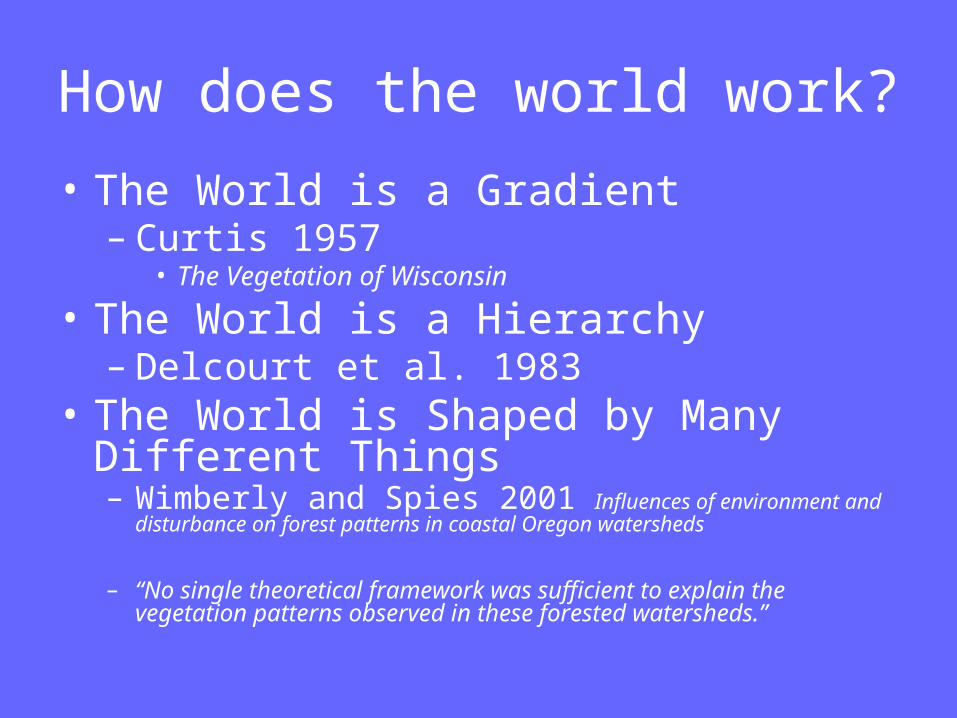
How does the world work?

• The World is a Gradient– Curtis 1957

• The Vegetation of Wisconsin

• The World is a Hierarchy– Delcourt et al. 1983

• The World is Shaped by Many Different Things– Wimberly and Spies 2001 Influences of environment and

disturbance on forest patterns in coastal Oregon watersheds

– “No single theoretical framework was sufficient to explain the vegetation patterns observed in these forested watersheds.”

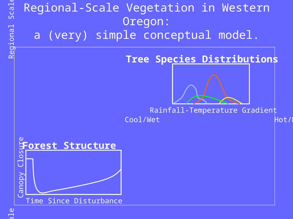
Regional-Scale Vegetation in Western Oregon:a (very) simple conceptual model.

Tree Species Distributions

Rainfall-Temperature GradientCool/Wet Hot/Dry

Loca

l Sca

le

Reg

iona

l Sca

le

Short-term Long-term

Forest Structure

Can

opy

Clo

sure

Time Since Disturbance

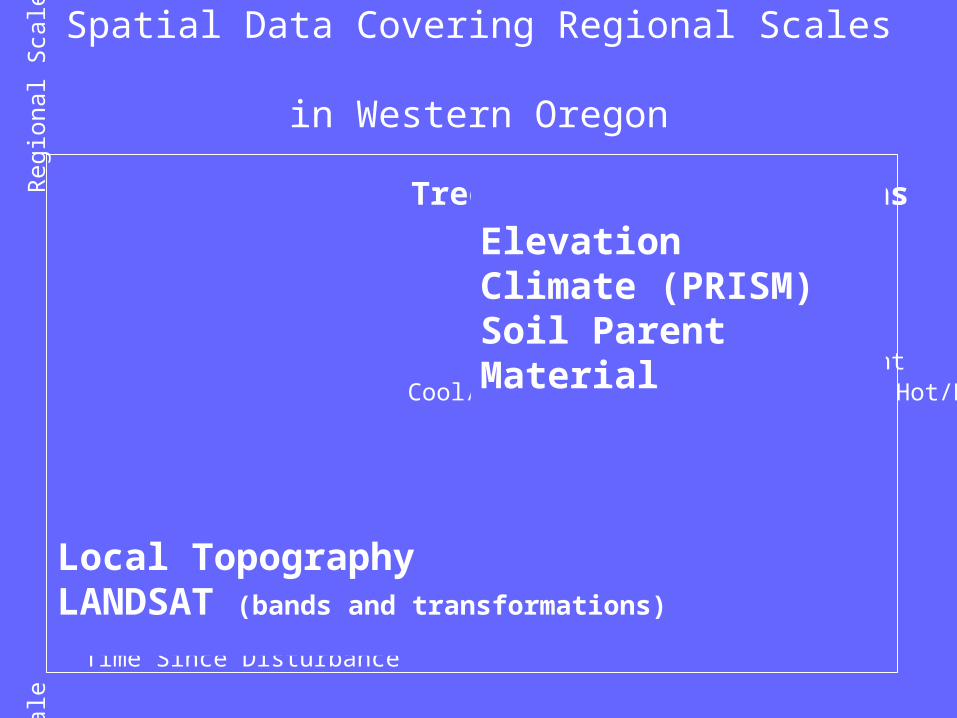
Spatial Data Covering Regional Scales in Western Oregon

Tree Species Distributions

Rainfall-Temperature GradientCool/Wet Hot/Dry

Loca

l Sca

le

Reg

iona

l Sca

le

Short-term Long-term

Forest Structure

Can

opy

Clo

sure

Time Since Disturbance

ElevationClimate (PRISM)Soil Parent Material

Local TopographyLANDSAT (bands and transformations)

Our Quest

• Make a highly accurate regional-scale vegetation map, that simultaneously represents detailed forest composition and structure.

• Peril #1:– The world is a complex place.

• Solution #1:– Use statistical models to sort out the complexity, and make a

prediction.

• Peril #2:– Statistical models often come with ASSUMPTIONS that cause

problems when violated.

• Solution #2:– Try to find a model with reasonable assumptions.– See whether it works any better than other methods.

Perils

You Are Here

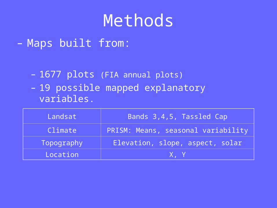
Methods– Maps built from:

– 1677 plots (FIA annual plots)

– 19 possible mapped explanatory variables.

Landsat Bands 3,4,5, Tassled Cap

Climate PRISM: Means, seasonal variability

Topography Elevation, slope, aspect, solar

Location X, Y

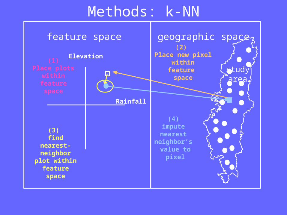
studyarea

(2) Place new pixel

withinfeature space

(3) find nearest-neighbor plot within feature

space

(4) impute nearest

neighbor’s value to

pixel

Methods: k-NN

feature space geographic space

Elevation

Rainfall

(1)Place plots

within feature space

(2) calculate

axis scores of pixel from

mapped data layersstudyarea

(3) find nearest-

neighbor plot in

gradient space

(4) impute nearest

neighbor’s value to

pixel

Methods: GNNgradient space geographic space

CCAAxis 2

(e.g., Temperature, Elevation)

CCAAxis 1

(e.g., Rainfall, local

topography)

(1)conductgradient

analysis ofplot data

ASSUMPTION: Species exhibit unimodal responses to environmental variables.

studyarea

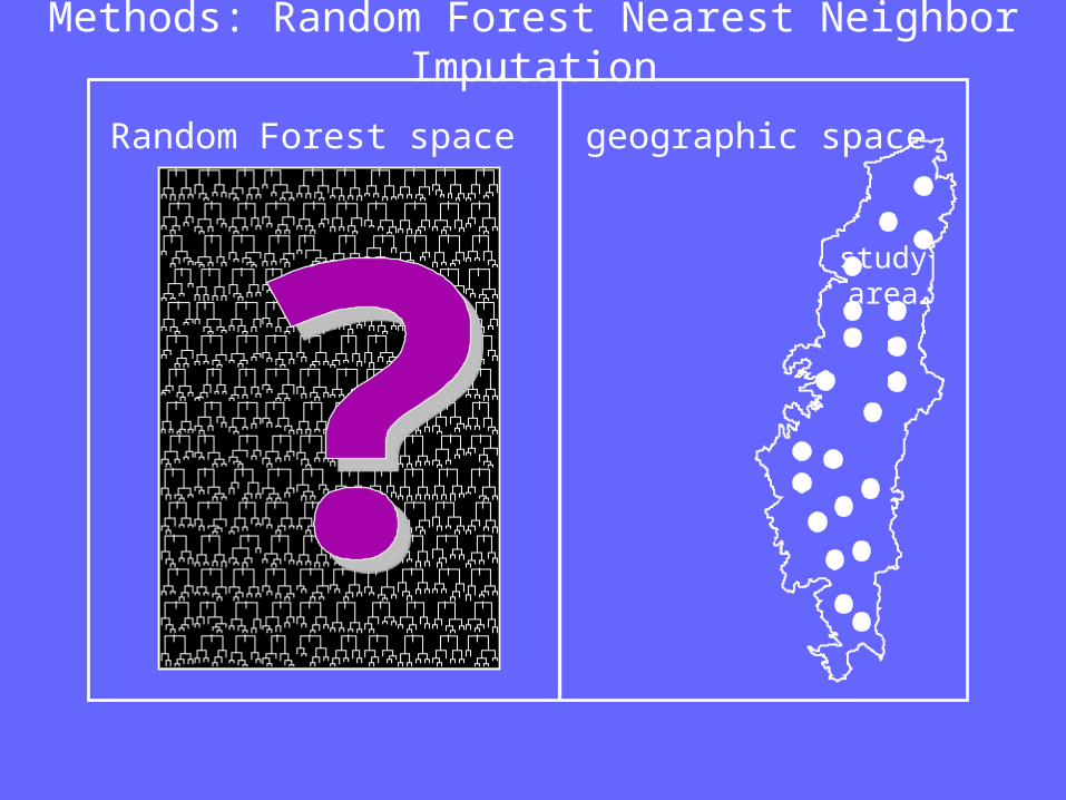
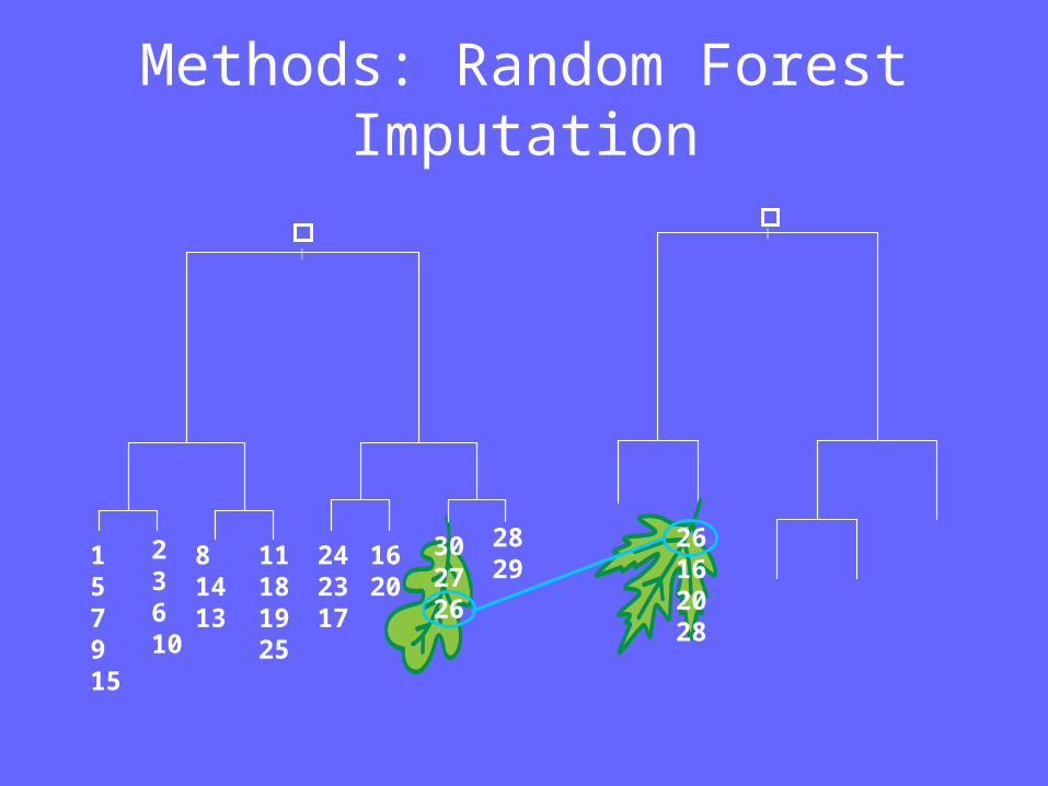
Methods: Random Forest Nearest Neighbor Imputation

Random Forest space geographic space

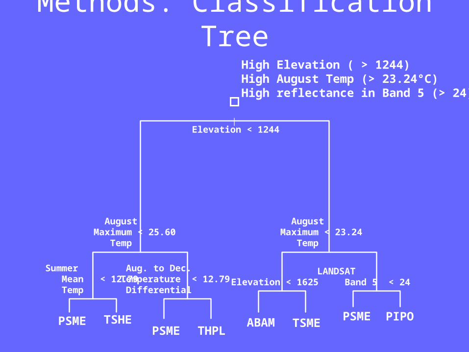
Methods: Classification Tree

|Elevation < 1244

August Maximum < 23.24 Temp

August Maximum < 25.60 Temp

Summer Mean < 12.79 Temp

Aug. to Dec. Temperature < 12.79 Differential

Elevation < 1625LANDSAT Band 5 < 24

PSME TSHEPSME THPL

ABAM TSMEPSME PIPO

High Elevation ( > 1244)High August Temp (> 23.24°C)High reflectance in Band 5 (> 24)

Methods: Random Forest

• A “Forest” of classification trees.

• Each tree is built from a random subset of plots and variables.

|ANNHDD < 4271.43

SMRPRE < 5535.09

X < 8808.88ANNHDD < 3950.45

SMRPRE < 5576.65

SMRTP < 2088.19

MR4300 < 166.968

ANNHDD < 4779.98

4215 4222 4224 4224

4228

4267 42154272 4228

|ANNTMP < 665.874

ANNVP < 591.82

ANNHDD < 4710.98X < 7248.68

STRATUS < 3.7435

X < 7762.43 X < 6340.86

ANNHDD < 3901.34215 42284215 4272

4215 4205

4224

4226 4224

|ANNGDD < 2578.11

ANNVP < 591.82

ANNGDD < 2190.48

ANNPRE < 740.947

STRATUS < 40.8768

R5400 < 117.208

ANNGDD < 3028.96

4228 4215

4272

4215 42154224

4224 4224

|ANNFROST < 1693.8

ANNFROST < 1271.82

CONTPRE < 788.967IDSURVEY < 456

ANNFROST < 2051.42

IDSURVEY < 423ADR5700 < 70.8343

4224 4224 4224 4224

4215 4272 4267 4228

|SMRTMP < 1206.3

ANNVP < 608.87

R5400 < 158.673

SMRTMP < 1105.53

ANNVP < 660.51

ANNVP < 610.822

TC200 < 134.347

SMRTMP < 1444.82

CONTPRE < 785.7484228 42154267

4272

4267 42154215

4224

4214 4224

|ANNHDD < 4204.74

DIFTMP < 2847.06

ANNHDD < 3669.42

CVPRE < 8079.84

DIFTMP < 3022.3

DIFTMP < 2854.2

SMRTMP < 1123.01SMRTMP < 1184.12

4226 42144224 4224 4215

4228 4272 4228 4215

|

Methods: Random Forest Imputation

|

157915

23610

81413

11181925

242317

1620

302726

2829

26162028

Accuracy Assessment

• Species Kappa

• RMSD

• Bray-Curtis Distance

Results

Pru

nu

s e

ma

rgin

ata

Ace

r g

lab

rum

La

rix

occ

ide

nta

lisT

axu

s b

revi

folia

Ch

ryso

lep

is c

hry

sop

hyl

laQ

ue

rcu

s d

ou

gla

sii

Ab

ies

pro

cera

Ca

loce

dru

s d

ecu

rre

ns

Arb

utu

s m

en

zie

sii

Th

uja

plic

ata

Ab

ies

con

colo

rP

inu

s co

nto

rta

Tsu

ga

he

tero

ph

ylla

Pse

ud

ots

ug

a m

en

zie

sii

Pru

nu

sO

TH

ER

Po

pu

lus

tre

mu

loid

es

Fra

xin

us

latif

olia

Co

rnu

s n

utta

llii

Pin

us

mo

ntic

ola

Ab

ies

x sh

ast

en

sis

Ab

ies

gra

nd

isP

inu

s la

mb

ert

ian

aA

lnu

s ru

bra

Ab

ies

lasi

oca

rpa

Qu

erc

us

ga

rrya

na

Jun

ipe

rus

occ

ide

nta

lisQ

ue

rcu

s ch

ryso

lep

isP

ice

a e

ng

elm

an

nii

Po

pu

lus

ba

lsa

mife

ra s

sp. t

rich

oca

rpa

Aln

us

rho

mb

ifolia

Ab

ies

ma

gn

ifica

Jun

ipe

rus

calif

orn

ica

Pin

us

alb

ica

ulis

Pin

us

atte

nu

ata

Pin

us

jeffr

eyi

No

Tre

es

Ce

rco

carp

us

led

ifoliu

sA

cer

ma

cro

ph

yllu

mP

inu

s sa

bin

ian

aP

inu

s p

on

de

rosa

Qu

erc

us

kello

gg

iiT

sug

a m

ert

en

sia

na

Ab

ies

am

ab

ilis

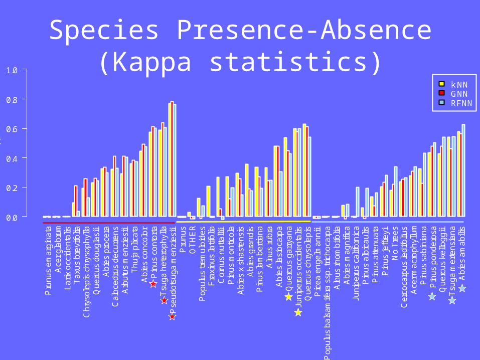
k.NNGNNRFNN

Ka

pp

a

0.0

0.2

0.4

0.6

0.8

1.0

Species Presence-Absence(Kappa statistics)

Forest Structure

Ba

sal A

rea

- L

arg

e

Ca

no

py

Co

ver

Ba

sal A

rea

- A

ll

Vo

lum

e -

All

Vo

lum

e -

La

rge

Vo

lum

e -

Sm

all

Ba

sal A

rea

- S

ma

ll

Sca

led

RM

SD

0.0

0.2

0.4

0.6

0.8

1.0

k-NNGNNRFNN

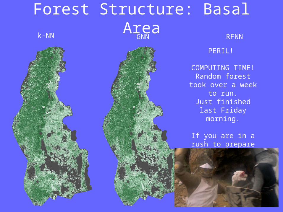
Forest Structure: Basal Areak-NN GNN RFNN

PERIL!

COMPUTING TIME! Random forest took over a week to run.

Just finished last Friday morning.

If you are in a rush to prepare for a

conference, don’t take this route!!!

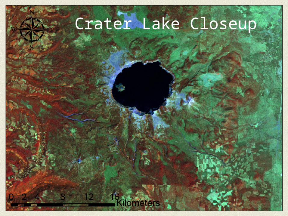
Crater Lake Closeup

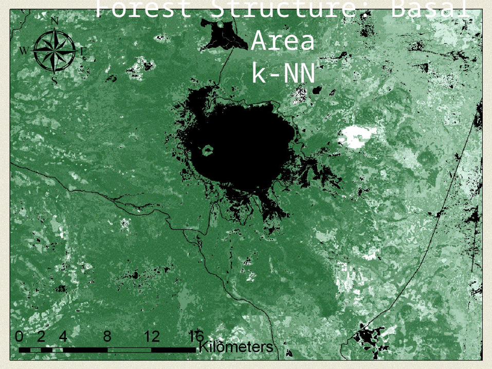
Forest Structure: Basal Areak-NN

Forest Structure: Basal AreaGNN

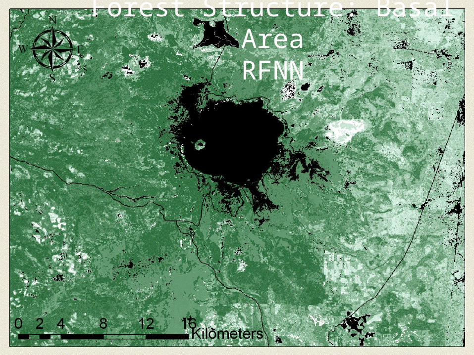
Forest Structure: Basal AreaRFNN

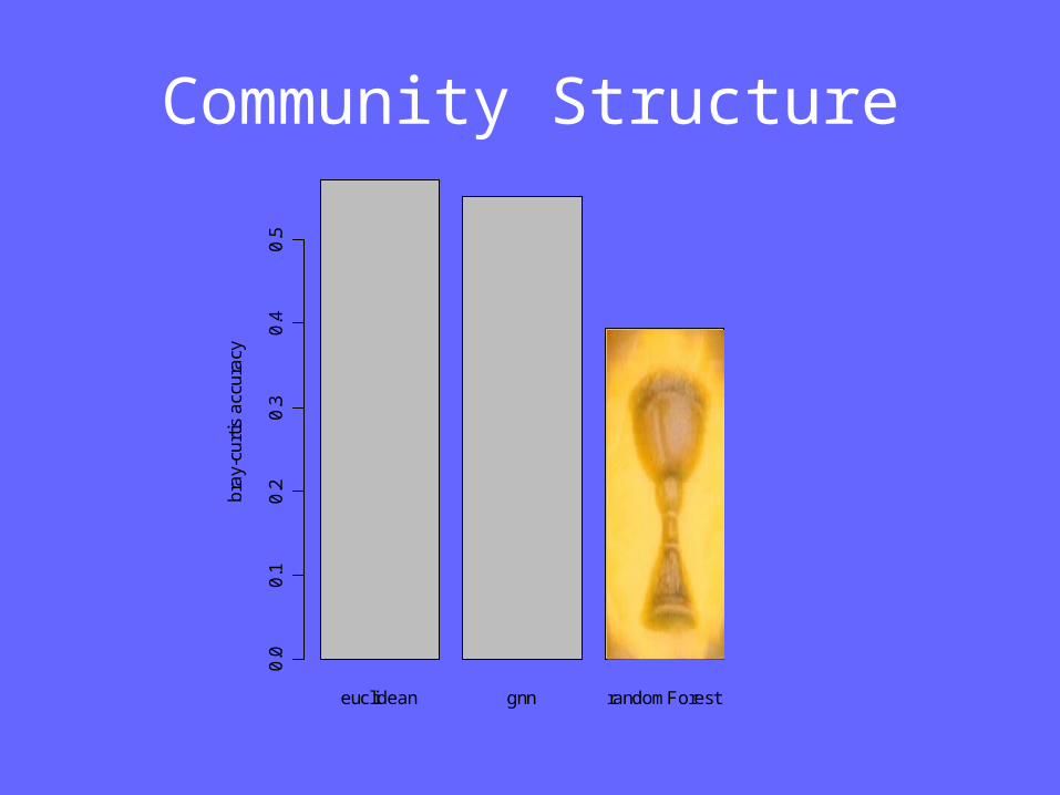
Community Structure

euclidean gnn randomForest

bra

y-cu

rtis

acc

ura

cy

0.0

0.1

0.2

0.3

0.4

0.5

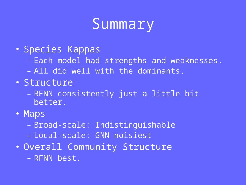
Summary

• Species Kappas– Each model had strengths and weaknesses.– All did well with the dominants.

• Structure– RFNN consistently just a little bit better.

• Maps– Broad-scale: Indistinguishable– Local-scale: GNN noisiest

• Overall Community Structure– RFNN best.

Conclusion

• Random forest did the best all around. broad-scale (species composition)

AND

local-scale (structure)

But, there’s still room for improvement.

Acknowledgements