Gradient descent GAN optimization is locally stable

Vaishnavh NagarajanComputer Science Department

Carnegie-Mellon UniversityPittsburgh, PA 15213

vaishnavh@cs.cmu.edu

J. Zico KolterComputer Science Department

Carnegie-Mellon UniversityPittsburgh, PA 15213zkolter@cs.cmu.edu

Abstract

Despite the growing prominence of generative adversarial networks (GANs), op-timization in GANs is still a poorly understood topic. In this paper, we analyzethe “gradient descent” form of GAN optimization, i.e., the natural setting wherewe simultaneously take small gradient steps in both generator and discriminatorparameters. We show that even though GAN optimization does not correspond to aconvex-concave game (even for simple parameterizations), under proper conditions,equilibrium points of this optimization procedure are still locally asymptoticallystable for the traditional GAN formulation. On the other hand, we show that therecently proposed Wasserstein GAN can have non-convergent limit cycles nearequilibrium. Motivated by this stability analysis, we propose an additional regular-ization term for gradient descent GAN updates, which is able to guarantee localstability for both the WGAN and the traditional GAN, and also shows practicalpromise in speeding up convergence and addressing mode collapse.

1 Introduction

Since their introduction a few years ago, Generative Adversarial Networks (GANs) [Goodfellow et al.,2014] have gained prominence as one of the most widely used methods for training deep generativemodels. GANs have been successfully deployed for tasks such as photo super-resolution, objectgeneration, video prediction, language modeling, vocal synthesis, and semi-supervised learning,amongst many others [Ledig et al., 2017, Wu et al., 2016, Mathieu et al., 2016, Nguyen et al., 2017,Denton et al., 2015, Im et al., 2016].

At the core of the GAN methodology is the idea of jointly training two networks: a generator network,meant to produce samples from some distribution (that ideally will mimic examples from the datadistribution), and a discriminator network, which attempts to differentiate between samples fromthe data distribution and the ones produced by the generator. This problem is typically written as amin-max optimization problem of the following form:

min

G

max

D

(Ex⇠p

data

[logD(x)] + Ez⇠p

latent

[log(1�D(G(z)))]) . (1)

For the purposes of this paper, we will shortly consider a more general form of the optimization prob-lem, which also includes the recent Wasserstein GAN (WGAN) [Arjovsky et al., 2017] formulation.

Despite their prominence, the actual task of optimizing GANs remains a challenging problem, bothfrom a theoretical and a practical standpoint. Although the original GAN paper included someanalysis on the convergence properties of the approach [Goodfellow et al., 2014], it assumed thatupdates occurred in pure function space, allowed arbitrarily powerful generator and discriminatornetworks, and modeled the resulting optimization objective as a convex-concave game, thereforeyielding well-defined global convergence properties. Furthermore, this analysis assumed that thediscriminator network is fully optimized between generator updates, an assumption that does notmirror the practice of GAN optimization. Indeed, in practice, there exist a number of well-documentedfailure modes for GANs such as mode collapse or vanishing gradient problems.

31st Conference on Neural Information Processing Systems (NIPS 2017), Long Beach, CA, USA.

Our contributions. In this paper, we consider the “gradient descent” formulation of GAN opti-mization, the setting where both the generator and the discriminator are updated simultaneously viasimple (stochastic) gradient updates; that is, there are no inner and outer optimization loops, andneither the generator nor the discriminator are assumed to be optimized to convergence. Despite thefact that, as we show, this does not correspond to a convex-concave optimization problem (even forsimple linear generator and discriminator representations), we show that:

Under suitable conditions on the representational powers of the discriminator and the generator,the resulting GAN dynamical system is locally exponentially stable.

That is, for some region around an equilibrium point of the updates, the gradient updates will convergeto this equilibrium point at an exponential rate. Interestingly, our conditions can be satisfied by thetraditional GAN but not by the WGAN, and we indeed show that WGANs can have non-convergentlimit cycles in the gradient descent case.

Our theoretical analysis also suggests a natural method for regularizing GAN updates by addingan additional regularization term on the norm of the discriminator gradient. We show that theaddition of this term leads to locally exponentially stable equilibria for all classes of GANs, includingWGANs. The additional penalty is highly related to (but also notably different from) recent proposalsfor practical GAN optimization, such as the unrolled GAN [Metz et al., 2017] and the improvedWasserstein GAN training [Gulrajani et al., 2017]. In practice, the approach is simple to implement,and preliminary experiments show that it helps avert mode collapse and leads to faster convergence.

2 Background and related work

GAN optimization and theory. Although the theoretical analysis of GANs has been far outpacedby their practical application, there have been some notable results in recent years, in additionto the aforementioned work in the original GAN paper. For the most part, this work is entirelycomplementary to our own, and studies a very different set of questions. Arjovsky and Bottou [2017]provide important insights into instability that arises when the supports of the generated distributionand the true distribution are disjoint. In contrast, in this paper we delve into an equally importantquestion of whether the updates are stable even when the generator is in fact very close to the truedistribution (and we answer in the affirmative). Arora et al. [2017], on the other hand, explorequestions relating to the sample complexity and expressivity of the GAN architecture, and theirrelation to the existence of an equilibrium point. However, it is still unknown as to whether, giventhat an equilibrium exists, the GAN update procedure will converge locally.

From a more practical standpoint, there have been a number of papers that address the topic ofoptimization in GANs. Several methods have been proposed that introduce new objectives orarchitectures for improving the (practical and theoretical) stability of GAN optimization [Arjovskyet al., 2017, Poole et al., 2016]. A wide variety of optimization heuristics and architectures havealso been proposed to address challenges such as mode collapse [Salimans et al., 2016, Metz et al.,2017, Che et al., 2017, Radford et al., 2016]. Our own proposed regularization term falls underthis same category, and hopefully provides some context for understanding some of these methods.Specifically, our regularization term (motivated by stability analysis) captures a degree of “foresight”of the generator in the optimization procedure, similar to the unrolled GANs procedure [Metz et al.,2017]. Indeed, we show that our gradient penalty is closely related to 1-unrolled GANs, but alsoprovides more flexibility in leveraging this foresight. Finally, gradient-based regularization has beenexplored for GANs, with one of the most recent works being that of Gulrajani et al. [2017], thoughtheir penalty is on the discriminator rather than the generator as in our case.

Finally, there are several works that have concurrently addressed similar issues as this paper. Ofparticular similarity to the methodology we propose here are the works by Roth et al. [2017] andMescheder et al. [2017]. The first of these two presents a stabilizing regularizer that is based on agradient norm, where the gradient is calculated with respect to the datapoints. Our regularizer on theother hand is based on the norm of a gradient calculated with respect to the parameters. Our approachhas some strong similarities with that of the second work noted above; however, the authors theredo not establish or disprove stability, and instead note the presence of zero eigenvalues (which wewill treat in some depth) as a motivation for their alternative optimization method. Thus, we feel theworks as a whole are quite complementary, and signify the growing interest in GAN optimizationissues.

2

Stochastic approximation algorithms and analysis of nonlinear systems. The technical toolswe use to analyze the GAN optimization dynamics in this paper come from the fields of stochasticapproximation algorithms and the analysis of nonlinear differential equations – notably the “ODEmethod” for analyzing convergence properties of dynamical systems [Borkar and Meyn, 2000,Kushner and Yin, 2003]. Consider a general stochastic process driven by the updates ✓

t+1

=

✓t

+ ↵t

(h(✓t

) + ✏t

) for vector ✓t

2 Rn, step size ↵t

> 0, function h : Rn ! Rn and a martingaledifference sequence ✏

t

.1 Under fairly general conditions, namely: 1) bounded second moments of ✏t

,2) Lipschitz continuity of h, and 3) summable but not square-summable step sizes, the stochasticapproximation algorithm converges to an equilibrium point of the (deterministic) ordinary differentialequation ˙✓(t) = h(✓(t)).

Thus, to understand stability of the stochastic approximation algorithm, it suffices to understandthe stability and convergence of the deterministic differential equation. Though such analysis istypically used to show global asymptotic convergence of the stochastic approximation algorithm toan equilibrium point (assuming the related ODE also is globally asymptotically stable), it can also beused to analyze the local asymptotic stability properties of the stochastic approximation algorithmaround equilibrium points.2 This is the technique we follow throughout this entire work, though forbrevity we will focus entirely on the analysis of the continuous time ordinary differential equation,and appeal to these standard results to imply similar properties regarding the discrete updates.

Given the above consideration, our focus will be on proving stability of the dynamical system aroundequilbrium points, i.e. points ✓? for which h(✓?

) = 0.3. Specifically, we appeal to the well knownlinearization theorem [Khalil, 1996, Sec 4.3], which states that if the Jacobian of the dynamicalsystem J = @h(✓)/@✓|

✓=✓

? evaluated at an equilibrium point is Hurwitz (has all strictly negativeeigenvalues, Re(�

i

(J)) < 0, 8i = 1, . . . , n), then the ODE will converge to ✓? for some non-emptyregion around ✓?, at an exponential rate. This means that the system is locally asymptotically stable,or more precisely, locally exponentially stable (see Definition A.1 in Appendix A).

Thus, an important contribution of this paper is a proof of this seemingly simple fact: under someconditions, the Jacobian of the dynamical system given by the GAN update is a Hurwitz matrix atan equilibrium (or, if there are zero-eigenvalues, if they correspond to a subspace of equilibria, thesystem is still asymptotically stable). While this is a trivial property to show for convex-concavegames, the fact that the GAN is not convex-concave leads to a substantially more challenging analysis.

In addition to this, we provide an analysis that is based on Lyapunov’s stability theorem (describedin Appendix A). The crux of the idea is that to prove convergence it is sufficient to identify a non-negative “energy” function for the linearized system which always decreases with time (specifically,the energy function will be a distance from the equilibrium, or from the subspace of equilibria). Mostimportantly, this analysis provides insights into the dynamics that lead to GAN convergence.

3 GAN optimization dynamics

This section comprises the main results of this paper, showing that under proper conditions thegradient descent updates for GANs (that is, updating both the generator and discriminator locally andsimultaneously) is locally exponentially stable around “good” equilibrium points (where “good” willbe defined shortly). This requires that the GAN loss be strictly concave, which is not the case forWGANs, and we indeed show that the updates for WGANs can cycle indefinitely. This leads us topropose a simple regularization term that is able to guarantee exponential stability for any concaveGAN loss, including the WGAN, rather than requiring strict concavity.

1Stochastic gradient descent on an objective f(✓) can be expressed in this framework as h(✓) = r✓f(✓).2Note that the local analysis does not show that the stochastic approximation algorithm will necessarily

converge to an equilibrium point, but still provides a valuable characterization of how the algorithm will behavearound these points.

3Note that this is a slightly different usage of the term equilibrium as typically used in the GAN literature,where it refers to a Nash equilibrium of the min-max optimization problem. These two definitions (assuming wemean just a local Nash equilibrium) are equivalent for the ODE corresponding to the min-max game, but we usethe dynamical systems meaning throughout this paper, that is, any point where the gradient update is zero.

3

3.1 The generalized GAN setting

For the remainder of the paper, we consider a slightly more general formulation of the GANoptimization problem than the one presented earlier, given by the following min/max problem:

min

G

max

D

V (G,D) = (Ex⇠p

data

[f(D(x))] + Ez⇠p

latent

[f(�D(G(z)))]) (2)

where G : Z ! X is the generator network, which maps from the latent space Z to the input spaceX ; D : X ! R is the discriminator network, which maps from the input space to a classificationof the example as real or synthetic; and f : R ! R is a concave function. We can recover thetraditional GAN formulation [Goodfellow et al., 2014] by taking f to be the (negated) logistic lossf(x) = � log(1 + exp(�x)); note that this convention slightly differs from the standard formulationin that in this case the discriminator outputs the real-valued “logits” and the loss function wouldimplicitly scale this to a probability. We can recover the Wasserstein GAN by simply taking f(x) = x.

Assuming the generator and discriminator networks to be parameterized by some set of parameters,✓D

and ✓G

respectively, we analyze the simple stochastic gradient descent approach to solving thisoptimization problem. That is, we take simultaneous gradient steps in both ✓

D

and ✓G

, which in our“ODE method” analysis leads to the following differential equation:

˙✓D

= r✓DV (✓G

,✓D

), ˙✓G

:= r✓GV (✓G

,✓D

). (3)

A note on alternative updates. Rather than updating both the generator and discriminator accord-ing to the min-max problem above, Goodfellow et al. [2014] also proposed a modified update forjust the generator that minimizes a different objective, V 0

(G,D) = �Ez⇠p

latent

[f(D(G(z)))] (thenegative sign is pulled out from inside f ). In fact, all the analyses we consider in this paper applyequally to this case (or any convex combination of both updates), as the ODE of the update equationshave the same Jacobians at equilibrium.

3.2 Why is proving stability hard for GANs?

Before presenting our main results, we first highlight why understanding the local stability of GANsis non-trivial, even when the generator and discriminator have simple forms. As stated above, GANoptimization consists of a min-max game, and gradient descent algorithms will converge if the gameis convex-concave – the objective must be convex in the term being minimized and concave in theterm being maximized. Indeed, this was a crucial assumption in the convergence proof in the originalGAN paper. However, for virtually any parameterization of the real GAN generator and discriminator,even if both representations are linear, the GAN objective will not be a convex-concave game:

Proposition 3.1. The GAN objective in Equation 2 can be a concave-concave objective, i.e., concavewith respect to both the discriminator and generator parameters, for a large part of the discriminatorspace, including regions arbitrarily close to the equilibrium.

To see why, consider a simple GAN over 1-dimensional data and latent space with linear generatorand discriminator, i.e. D(x) = ✓

D

x+ ✓0D

and G(z) = ✓G

z + ✓0G

. Then the GAN objective is:V (G,D) = E

x⇠p

data

[f(✓D

x+ ✓0D

)] + Ez⇠p

latent

[f(�✓D

(✓G

z + ✓0G

)� ✓0D

)].

Because f is concave, by inspection we can see that V is concave in ✓D

and ✓0D

; but it is alsoconcave (not convex) in ✓

G

and ✓0G

, for the same reason. Thus, the optimization involves concaveminimization, which in general is a difficult problem. To prove that this is not a peculiarity of theabove linear discriminator system, in Appendix B, we show similar observations for a more generalparametrization, and also for the case where f 00

(x) = 0 (which happens in the case of WGANs).

Thus, a major question remains as to whether or not GAN optimization is stable at all (most concavemaximization is not). Indeed, there are several well-known properties of GAN optimization that maymake it seem as though gradient descent optimization may not work in theory. For instance, it iswell-known that at the optimal location p

g

= pdata

, the optimal discriminator will output zero on allexamples, which in turn means that any generator distribution will be optimal for this generator. Thiswould seem to imply that the system can not be stable around such an equilibrium.

However, as we will show, gradient descent GAN optimization is locally asymptotically stable, evenfor natural parameterizations of generator-discriminator pairs (which still make up concave-concaveoptimization problems). Furthermore, at equilibrium, although the zero-discriminator propertymeans that the generator is not stable “independently”, the joint dynamical system of generator anddiscriminator is locally asymptotically stable around certain equilibrium points.

4

3.3 Local stability of general GAN systems

This section contains our first technical result, establishing that GANs are locally stable under properlocal conditions. Although the proofs are deferred to the appendix, the elements that we do emphasizehere are the conditions that we identified for local stability to hold. Indeed, because the proof rests onthese conditions (some of which are fairly strong), we want to highlight them as much as possible, asthey themselves also convey valuable intuition as to what is required for GAN convergence.

To formalize our conditions, we denote the support of a distribution with probability density function(p.d.f) p by supp(p) and the p.d.f of the generator ✓

G

by p✓G . Let B✏

(·) denote the Euclidean L2

-ballof radius of ✏. Let �

max

(·) and �(+)

min

(·) denote the largest and the smallest non-zero eigenvalues of anon-zero positive semidefinite matrix. Let Col(·) and Null(·) denote the column space and null spaceof a matrix respectively. Finally, we define two key matrices that will be integral to our analyses:

K

DD

, Ep

data

[r✓DD✓D(x)rT

✓DD✓D(x)]

��✓?D, K

DG

,Z

Xr✓DD✓D(x)rT

✓Gp✓G(x)dx

����(✓?

D,✓?G)

.

Here, the matrices are evaluated at an equilibrium point (✓?D

,✓?G

) which we will characterize shortly.The significance of these terms is that, as we will see, K

DD

is proportional to the Hessian of theGAN objective with respect to the discriminator parameters at equilibrium, and K

DG

is proportionalto the off-diagonal term in this Hessian, corresponding to the discriminator and generator parameters.These matrices also occur in similar positions in the Jacobian of the system at equilibrium.

We now discuss conditions under which we can guarantee exponential stability. All our conditionsare imposed on both (✓?

D

,✓?G

) and all equilibria in a small neighborhood around it, though we donot state this explicitly in every assumption. First, we define the “good” equilibria we care about asthose that correspond to a generator which matches the true distribution and a discriminator that isidentically zero on the support of this distribution. As described next, implicitly, this also assumesthat the discriminator and generator representations are powerful enough to guarantee that there areno “bad” equilibria in a local neighborhood of this equilibrium.

Assumption I. p✓?G= p

data

and D✓?D(x) = 0, 8 x 2 supp(p

data

).

The assumption that the generator matches the true distribution is a rather strong assumption, asit limits us to the “realizable” case, where the generator is capable of creating the underlying datadistribution. Furthermore, this means the discriminator is (locally) powerful enough that for any othergenerator distribution it is not at equilibrium (i.e., discriminator updates are non-zero). Since wedo not typically expect this to be the case, we also provide an alternative non-realizable assumptionbelow that is also sufficient for our results, i.e., the system is still stable. In both the realizable andnon-realizable cases the requirement of an all-zero discriminator remains. This implicitly requireseven the generator representation be (locally) rich enough so that when the discriminator is notidentically zero, the generator is not at equilibrium (i.e., generator updates are non-zero). Finally,note that these conditions do not disallow bad equilibria outside of this neighborhood, which maypotentially even be unstable.

Assumption I. (Non-realizable) The discriminator is linear in its parameters ✓D

and furthermore,for any equilibrium point (✓?

D

,✓?G

), D✓?D(x) = 0, 8 x 2 supp(p

data

) [ supp(p✓?G).

This alternative assumption is largely a weakening of Assumption I, as the condition on the dis-criminator remains, but there is no requirement that the generator give rise to the true distribution.However, the requirement that the discriminator be linear in the parameters (not in its input) is anadditional restriction that seems unavoidable in this case for technical reasons. Further, note thatthe fact that D✓?

D(x) = 0 and that the generator/discriminator are both at equilibrium, still means

that although it may be that p✓?G6= p

data

, these distributions are (locally) indistinguishable as far asthe discriminator is concerned. Indeed, this is a nice characterization of “good” equilibria that thediscriminator cannot differentiate between the real and generated samples.

Our goal next is to identify strong curvature conditions that can be imposed on the objective V (ora function related to the objective), though only locally at equilibrium. First, we will require thatthe objective is strongly concave in the discriminator parameter space at equilibrium (note that it isconcave by default). However, on the other hand, we cannot require the objective to be strongly convexin the generator parameter space as we saw that the objective is not convex-concave even in the nicestscenario, even arbitrarily close to equilbrium. Instead, we identify another convex function, namely

5

the magnitude of the update on the equilibrium discriminator, i.e., k r✓DV (✓D

,✓G

)|✓D=✓?Dk2, and

require that to be strongly convex in the generator space at equilibrium. Since these strong curvatureassumptions will allow only systems with a locally unique equilibrium, we will state them in a relaxedform that accommodates a local subspace of equilibria. Furthermore, we will state these assumptionsin two parts, first as a condition on f and second as a condition on the parameter space.

First, the condition on f is straightforward, making it necessary that the loss f be concave at 0; as wewill show, when this condition is not met, there need not be local asymptotic convergence.

Assumption II. The function f satisfies f 00(0) < 0, and f 0

(0) 6= 0.

Next, to state conditions on the parameter space while also allowing systems with multiple equilibrialocally, we first define the following property for a function, say g, at a specific point in its domain:along any direction, either the second derivative of g must be non-zero or all derivatives must be zero.For example, at the origin, g(x, y) = x2

+ x2y2 is flat along y, and along any other direction at anangle ↵ 6= 0 with the y axis, the second derivative is 2 sin2 ↵. For the GAN system, we will requirethis property, formalized in Property I, for two convex functions whose Hessians are proportional toK

DD

and K

T

DG

K

DG

. We provide more intuition for these functions below.

Property I. g : ⇥ ! R satisfies Property I at ✓? 2 ⇥ if for any ✓ 2 Null(r2

✓g(✓)��✓?), the function

is locally constant along ✓ at ✓?, i.e., 9✏ > 0 such that for all ✏0 2 (�✏, ✏), g(✓?) = g(✓?

+ ✏0✓).

Assumption III. At an equilibrium (✓?D

,✓?G

), the functions Ep

data

[D2

✓D(x)] and

���Ep

data

[r✓DD✓D(x)]� Ep✓G

[r✓DD✓D(x)]���2

����✓D=✓?

D

must satisfy Property I in the discriminator

and generator space respectively.

Here is an intuitive explanation of what these two non-negative functions represent and how they relateto the objective. The first function is a function of ✓

D

which measures how far ✓D

is from an all-zerostate, and the second is a function of ✓

G

which measures how far ✓G

is from the true distribution; atequilibrium these functions are zero. We will see later that given f 00

(0) < 0, the curvature of the firstfunction at ✓?

D

is representative of the curvature of V (✓D

,✓?G

) in the discriminator space; similarly,given f 0

(0) 6= 0 the curvature of the second function at ✓?G

is representative of the curvature of themagnitude of the discriminator update on ✓?

D

in the generator space. The intuition behind why thisparticular relation holds is that, when ✓

G

moves away from the true distribution, while the secondfunction in Assumption III increases, ✓?

D

also becomes more suboptimal for that generator; as a result,the magnitude of update on ✓?

D

increases too. Note that we show in Lemma C.2 that the Hessian ofthe two functions in Assumption III in the discriminator and the generator space respectively areproportional to K

DD

and K

T

DG

K

DG

.

The above relations involving the two functions and the GAN objective, together with Assumption III,basically allow us to consider systems with reasonable strong curvature properties, while alsoallowing many equilibria in a local neighborhood in a specific sense. In particular, if the curvatureof the first function is flat along a direction u (which also means that K

DD

u = 0) we can perturb✓?D

slightly along u and still have an ‘equilibrium discriminator’ as defined in Assumption I, i.e.,8x 2 supp(p✓?

G), D✓D(x) = 0. Similarly, for any direction v along which the curvature of the

second function is flat (i.e., KDG

v = 0), we can perturb ✓?G

slightly along that direction such that✓G

remains an ‘equilibrium generator’ as defined in Assumption I, i.e., p✓G = p

data

. We prove thisformally in Lemma C.2. Perturbations along any other directions do not yield equilibria becausethen, either ✓

D

is no longer in an all-zero state or ✓G

does not match the true distribution. Thus, weconsider a setup where the rank deficiencies of K

DD

and K

T

DG

K

DG

if any, correspond to equivalentequilibria (which typically exist for neural networks, though in practice they may not correspond to‘linear’ perturbations as modeled here).

Our final assumption is on the supports of the true and generated distributions: we require that all thegenerators in a sufficiently small neighborhood of the equilibrium have distributions with the samesupport as the true distribution. Following this, we briefly discuss a relaxation of this assumption.

Assumption IV. 9✏G

> 0 such that 8✓G

2 B✏G(✓

?G

), supp(p✓G) = supp(pdata

).

This may typically hold if the support covers the whole space X ; but when the true distribution hassupport in some smaller disjoint parts of the space X , nearby generators may correspond to slightly

6

displaced versions of this distribution with a different support. For the latter scenario, we show inAppendix C.1 that local exponential stability holds under a certain smoothness condition on thediscriminator. Specifically, we require that D✓?

D(·) be zero not only on the support of ✓?

G

but alsoon the support of small perturbations of ✓?

G

as otherwise the generator will not be at equilibrium.(Additionally, we also require this property from the discriminators that lie within a small perturbationof ✓?

D

in the null space of KDD

so that they correspond to equilibrium discriminators.) We notethat while this relaxed assumption accounts for a larger class of examples, it is still strong in thatit also restricts us from certain simple systems. Due to space constraints, we state and discuss theimplications of this assumption in greater detail in Appendix C.1.

We now state our main result.

Theorem 3.1. The dynamical system defined by the GAN objective in Equation 2 and the updates inEquation 3 is locally exponentially stable with respect to an equilibrium point (✓?

D

,✓?G

) when theAssumptions I, II, III, IV hold for (✓?

D

,✓?G

) and other equilibria in a small neighborhood around it.Furthermore, the rate of convergence is governed only by the eigenvalues � of the Jacobian J of thesystem at equilibrium with a strict negative real part upper bounded as:

• If Im(�) = 0, then Re(�) 2f

00(0)f

02(0)�

(+)

min

(KDD)�

(+)

min

(K

TDGKDG)

4f

002(0)�

(+)

min

(KDD)�

max

(KDD)+f

0(0)

2

�

(+)

min

(K

TDGKDG)

• If Im(�) 6= 0, then Re(�) f 00(0)�

(+)

min

(K

DD

)

The vast majority of our proofs are deferred to the appendix, but we briefly describe the intuitionhere. It is straightforward to show that the Jacobian J of the system at equilibrium can be written as:

J =

J

DD

J

DG

�J

T

DG

J

GG

�=

2f 00

(0)K

DD

f 0(0)K

DG

�f 0(0)K

T

DG

0

�.

Recall that we wish to show this is Hurwitz. First note that JDD

(the Hessian of the objective withrespect to the discriminator) is negative semi-definite if and only if f 00

(0) < 0. Next, a crucialobservation is that J

GG

= 0 i.e, the Hessian term w.r.t. the generator vanishes because for the all-zerodiscriminator, all generators result in the same objective value. Fortunately, this means at equilibriumwe do not have non-convexity in ✓

G

precluding local stability. Then, we make use of the crucialLemma G.2 we prove in the appendix, showing that any matrix of the form

⇥�Q P; �P

T

0

⇤is

Hurwitz provided that �Q is strictly negative definite and P has full column rank.

However, this property holds only when K

DD

is positive definite and K

DG

is full column rank.Now, if K

DD

or KDG

do not have this property, recall that the rank deficiency is due to a subspaceof equilibria around (✓?

D

,✓?G

). Consequently, we can analyze the stability of the system projectedto an subspace orthogonal to these equilibria (Theorem A.4). Additionally, we also prove stabilityusing Lyapunov’s stability (Theorem A.1) by showing that the squared L

2

distance to the subspace ofequilibria always either decreases or only instantaneously remains constant.

Additional results. In order to illustrate our assumptions in Theorem 3.1, in Appendix D weconsider a simple GAN that learns a multi-dimensional Gaussian using a quadratic discriminator anda linear generator. In a similar set up, in Appendix E, we consider the case where f(x) = x, i.e., theWasserstein GAN, and so f 00

(x) = 0, and we show that the system can perennially cycle around anequilibrium point without converging. A simple two-dimensional example is visualized in Section 4.Thus, gradient descent WGAN optimization is not necessarily asymptotically stable.

3.4 Stabilizing optimization via gradient-based regularization

Motivated by the considerations above, in this section we propose a regularization penalty for thegenerator update, which uses a term based upon the gradient of the discriminator. Crucially, theregularization term does not change the parameter values at the equilibrium point, and at the sametime enhances the local stability of the optimization procedure, both in theory and practice. Althoughthese update equations do require that we differentiate with respect to a function of another gradientterm, such “double backprop” terms (see e.g., Drucker and Le Cun [1992]) are easily computed bymodern automatic differentiation tools. Specifically, we propose the regularized update

✓G

:= ✓G

� ↵r✓G

�V (D✓D , G✓G) + ⌘kr✓DV (D✓D , G✓G)k2

�. (4)

7

Local Stability The intuition of this regularizer is perhaps most easily understood by consideringhow it changes the Jacobian at equilibrium (though there are other means of motivating the update aswell, discussed further in Appendix F.2). In the Jacobian of the new update, although there are nownon-antisymmetric diagonal blocks, the block diagonal terms are now negative definite:

J

DD

J

DG

�J

T

DG

(I+ 2⌘JDD

) �2⌘JT

DG

J

DG

�.

As we show below in Theorem 3.2 (proved in Appendix F), as long as we choose ⌘ small enough sothat I + 2⌘J

DD

⌫ 0, this guarantees the updates are locally asymptotically stable for any concave f .In addition to stability properties, this regularization term also addresses a well known failure statein GANs called mode collapse, by lending more “foresight” to the generator. The way our updatesprovide this foresight is very similar to the unrolled updates proposed in Metz et al. [2017], althoughour regularization is much simpler and provides more flexibility to leverage the foresight. In practice,we see that our method can be as powerful as the more complex and slower 10-unrolled GANs. Wediscuss this and other intuitive ways of motivating our regularizer in Appendix F.

Theorem 3.2. The dynamical system defined by the GAN objective in Equation 2 and the updatesin Equation 4, is locally exponentially stable at the equilibrium, under the same conditions as inTheorem 3.1, if ⌘ < 1

2�

max

(�JDD)

. Further, under appropriate conditions similar to these, the WGANsystem is locally exponentially stable at the equilibrium for any ⌘. The rate of convergence for theWGAN is governed only by the eigenvalues � of the Jacobian at equilibrium with a strict negativereal part upper bounded as:

• If Im(�) = 0, then Re(�) � 2f

02(0)⌘�

(+)

min

(K

TDGKDG)

4f

02(0)⌘

2

�

max

(K

TDGKDG)+1

• If Im(�) 6= 0, then Re(�) �⌘f 02(0)�

(+)

min

(K

T

DG

K

DG

).

4 Experimental results

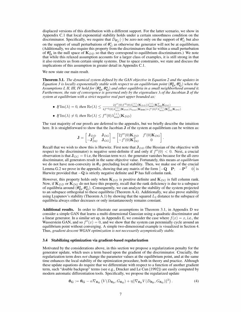
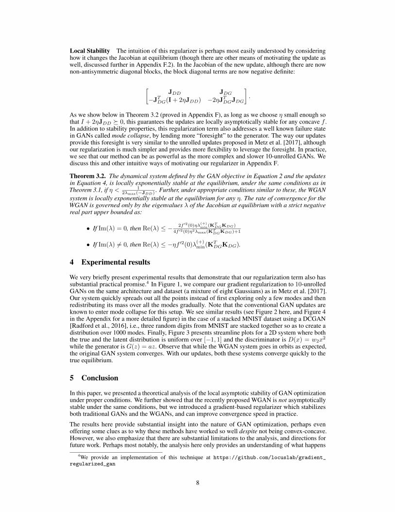
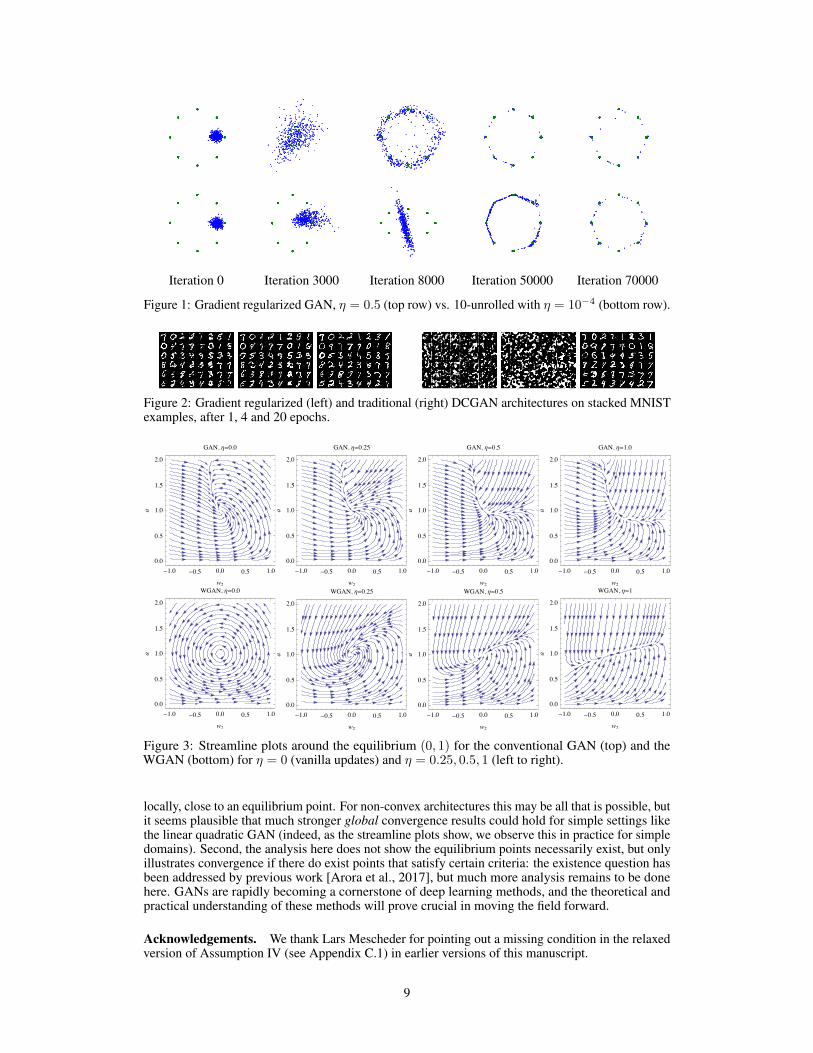
We very briefly present experimental results that demonstrate that our regularization term also hassubstantial practical promise.4 In Figure 1, we compare our gradient regularization to 10-unrolledGANs on the same architecture and dataset (a mixture of eight Gaussians) as in Metz et al. [2017].Our system quickly spreads out all the points instead of first exploring only a few modes and thenredistributing its mass over all the modes gradually. Note that the conventional GAN updates areknown to enter mode collapse for this setup. We see similar results (see Figure 2 here, and Figure 4in the Appendix for a more detailed figure) in the case of a stacked MNIST dataset using a DCGAN[Radford et al., 2016], i.e., three random digits from MNIST are stacked together so as to create adistribution over 1000 modes. Finally, Figure 3 presents streamline plots for a 2D system where boththe true and the latent distribution is uniform over [�1, 1] and the discriminator is D(x) = w

2

x2

while the generator is G(z) = az. Observe that while the WGAN system goes in orbits as expected,the original GAN system converges. With our updates, both these systems converge quickly to thetrue equilibrium.

5 Conclusion

In this paper, we presented a theoretical analysis of the local asymptotic stability of GAN optimizationunder proper conditions. We further showed that the recently proposed WGAN is not asymptoticallystable under the same conditions, but we introduced a gradient-based regularizer which stabilizesboth traditional GANs and the WGANs, and can improve convergence speed in practice.

The results here provide substantial insight into the nature of GAN optimization, perhaps evenoffering some clues as to why these methods have worked so well despite not being convex-concave.However, we also emphasize that there are substantial limitations to the analysis, and directions forfuture work. Perhaps most notably, the analysis here only provides an understanding of what happens

4We provide an implementation of this technique at https://github.com/locuslab/gradient_

regularized_gan

8

Iteration 0 Iteration 3000 Iteration 8000 Iteration 50000 Iteration 70000

Figure 1: Gradient regularized GAN, ⌘ = 0.5 (top row) vs. 10-unrolled with ⌘ = 10

�4 (bottom row).

Figure 2: Gradient regularized (left) and traditional (right) DCGAN architectures on stacked MNISTexamples, after 1, 4 and 20 epochs.

!1.0 !0.5 0.0 0.5 1.00.0

0.5

1.0

1.5

2.0

w2

a

GAN, Η#0.0

!1.0 !0.5 0.0 0.5 1.00.0

0.5

1.0

1.5

2.0

w2

a

WGAN, Η#0.0

!1.0 !0.5 0.0 0.5 1.00.0

0.5

1.0

1.5

2.0

w2

a

GAN, Η#0.25

!1.0 !0.5 0.0 0.5 1.00.0

0.5

1.0

1.5

2.0

w2

a

WGAN, Η#0.25

!1.0 !0.5 0.0 0.5 1.00.0

0.5

1.0

1.5

2.0

w2

a

GAN, Η#0.5

!1.0 !0.5 0.0 0.5 1.00.0

0.5

1.0

1.5

2.0

w2

a

WGAN, Η#0.5

!1.0 !0.5 0.0 0.5 1.00.0

0.5

1.0

1.5

2.0

w2

a

GAN, Η#1.0

!1.0 !0.5 0.0 0.5 1.00.0

0.5

1.0

1.5

2.0

w2

a

WGAN, Η#1

Figure 3: Streamline plots around the equilibrium (0, 1) for the conventional GAN (top) and theWGAN (bottom) for ⌘ = 0 (vanilla updates) and ⌘ = 0.25, 0.5, 1 (left to right).

locally, close to an equilibrium point. For non-convex architectures this may be all that is possible, butit seems plausible that much stronger global convergence results could hold for simple settings likethe linear quadratic GAN (indeed, as the streamline plots show, we observe this in practice for simpledomains). Second, the analysis here does not show the equilibrium points necessarily exist, but onlyillustrates convergence if there do exist points that satisfy certain criteria: the existence question hasbeen addressed by previous work [Arora et al., 2017], but much more analysis remains to be donehere. GANs are rapidly becoming a cornerstone of deep learning methods, and the theoretical andpractical understanding of these methods will prove crucial in moving the field forward.

Acknowledgements. We thank Lars Mescheder for pointing out a missing condition in the relaxedversion of Assumption IV (see Appendix C.1) in earlier versions of this manuscript.

9

ReferencesMartin Arjovsky and Léon Bottou. Towards principled methods for training generative adversarial

networks. In International Conference on Learning Representations (ICLR), 2017.

Martin Arjovsky, Soumith Chintala, and Léon Bottou. Wasserstein generative adversarial networks. InProceedings of the 34th International Conference on Machine Learning, volume 70 of Proceedingsof Machine Learning Research, pages 214–223, 2017.

Sanjeev Arora, Rong Ge, Yingyu Liang, Tengyu Ma, and Yi Zhang. Generalization and equilibriumin generative adversarial nets (GANs). In Proceedings of the 34th International Conference onMachine Learning, volume 70 of Proceedings of Machine Learning Research, pages 224–232,2017.

Vivek S Borkar and Sean P Meyn. The ode method for convergence of stochastic approximation andreinforcement learning. SIAM Journal on Control and Optimization, 38(2):447–469, 2000.

Tong Che, Yanran Li, Athul Paul Jacob, Yoshua Bengio, and Wenjie Li. Mode regularized generativeadversarial networks. In Fifth International Conference on Learning Representations (ICLR).2017.

Emily L Denton, Soumith Chintala, Arthur Szlam, and Rob Fergus. In Advances in Neural InformationProcessing Systems 28, pages 1486–1494. 2015.

Harris Drucker and Yann Le Cun. Improving generalization performance using double backpropaga-tion. IEEE Transactions on Neural Networks, 3(6):991–997, 1992.

Ian Goodfellow, Jean Pouget-Abadie, Mehdi Mirza, Bing Xu, David Warde-Farley, Sherjil Ozair,Aaron Courville, and Yoshua Bengio. Generative adversarial nets. In Advances in NeuralInformation Processing Systems 27, pages 2672–2680. 2014.

Ishaan Gulrajani, Faruk Ahmed, Martin Arjovsky, Vincent Dumoulin, and Aaron Courville. Improvedtraining of wasserstein GANs. In Thirty-first Annual Conference on Neural Information ProcessingSystems (NIPS). 2017.

Daniel Jiwoong Im, Chris Dongjoo Kim, Hui Jiang, and Roland Memisevic. Generating images withrecurrent adversarial networks. arXiv preprint arXiv:1602.05110, 2016.

Hassan K Khalil. Non-linear Systems. Prentice-Hall, New Jersey, 1996.

Harold Kushner and George Yin. Stochastic Approximation and Recursive Algorithms and Applica-tions, volume 35 of Stochastic Modelling and Applied Probability. Springer-Verlag New York,The address, 2003.

Christian Ledig, Lucas Theis, Ferenc Huszar, Jose Caballero, Andrew Cunningham, Alejandro Acosta,Andrew Aitken, Alykhan Tejani, Johannes Totz, Zehan Wang, and Wenzhe Shi. Photo-realisticsingle image super-resolution using a generative adversarial network. In The IEEE Conference onComputer Vision and Pattern Recognition (CVPR), July 2017.

Jan R Magnus, Heinz Neudecker, et al. Matrix differential calculus with applications in statistics andeconometrics. 1995.

Michael Mathieu, Camille Couprie, and Yann LeCun. Deep multi-scale video prediction beyondmean square error. In Fourth International Conference on Learning Representations (ICLR). 2016.

L. Mescheder, S. Nowozin, and A. Geiger. The numerics of GANs. In Thirty-first Annual Conferenceon Neural Information Processing Systems (NIPS). 2017.

Luke Metz, Ben Poole, David Pfau, and Jascha Sohl-Dickstein. Unrolled generative adversarialnetworks. In Fifth International Conference on Learning Representations (ICLR). 2017.

Anh Nguyen, Jeff Clune, Yoshua Bengio, Alexey Dosovitskiy, and Jason Yosinski. Plug & playgenerative networks: Conditional iterative generation of images in latent space. In The IEEEConference on Computer Vision and Pattern Recognition (CVPR), July 2017.

10

Ben Poole, Alexander A Alemi, Jascha Sohl-Dickstein, and Anelia Angelova. Improved generatorobjectives for GANs. arXiv preprint arXiv:1612.02780, 2016.

Alec Radford, Luke Metz, and Soumith Chintala. Unsupervised representation learning with deepconvolutional generative adversarial networks. In Fourth International Conference on LearningRepresentations (ICLR). 2016.

K. Roth, A. Lucchi, S. Nowozin, and T. Hofmann. Stabilizing training of generative adversarial net-works through regularization. In Thirty-first Annual Conference on Neural Information ProcessingSystems (NIPS). 2017.

Tim Salimans, Ian Goodfellow, Wojciech Zaremba, Vicki Cheung, Alec Radford, and Xi Chen.Improved techniques for training GANs. In Advances in Neural Information Processing Systems29, pages 2234–2242. 2016.

Jiajun Wu, Chengkai Zhang, Tianfan Xue, Bill Freeman, and Josh Tenenbaum. Learning a probabilis-tic latent space of object shapes via 3d generative-adversarial modeling. In Advances in NeuralInformation Processing Systems 29, pages 82–90. 2016.

11