Gradient Descent

Lecturer: Ryan TibshiraniConvex Optimization 10-725/36-725

Last time: canonical convex programs

• Linear program (LP): takes the form

minx

cTx

subject to Dx ≤ dAx = b

• Quadratic program (QP): like an LP, but with a quadraticcriterion

• Semidefinite program (SDP): like an LP, but with matrices

• Conic program: the most general form of all

2

Gradient descent

Consider unconstrained, smooth convex optimization

minx

f(x)

i.e., f is convex and differentiable with dom(f) = Rn. Denote theoptimal criterion value by f? = minx f(x), and a solution by x?

Gradient descent: choose initial point x(0) ∈ Rn, repeat:

x(k) = x(k−1) − tk · ∇f(x(k−1)), k = 1, 2, 3, . . .

Stop at some point

3

●

●

●

●

●

4

●

●

●

●

●

5

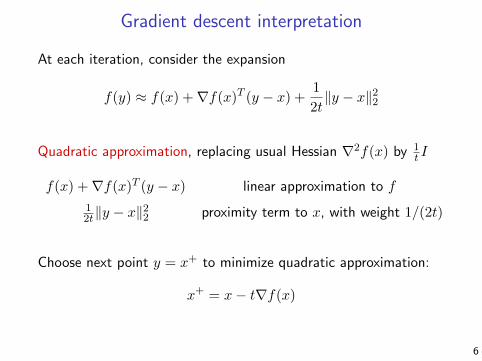
Gradient descent interpretation

At each iteration, consider the expansion

f(y) ≈ f(x) +∇f(x)T (y − x) +1

2t‖y − x‖22

Quadratic approximation, replacing usual Hessian ∇2f(x) by 1t I

f(x) +∇f(x)T (y − x) linear approximation to f

12t‖y − x‖22 proximity term to x, with weight 1/(2t)

Choose next point y = x+ to minimize quadratic approximation:

x+ = x− t∇f(x)

6

●

●

Blue point is x, red point is

x+ = argminy

f(x) +∇f(x)T (y − x) +1

2t‖y − x‖22

7

Outline

Today:

• How to choose step sizes

• Convergence analysis

• Gradient boosting

• Stochastic gradient descent

8

Fixed step size

Simply take tk = t for all k = 1, 2, 3, . . ., can diverge if t is too big.Consider f(x) = (10x21 + x22)/2, gradient descent after 8 steps:

−20 −10 0 10 20

−20

−10

010

20 ●

●

●

*

9

Can be slow if t is too small. Same example, gradient descent after100 steps:

−20 −10 0 10 20

−20

−10

010

20 ●●●●●●●●●●●●●●●●●●●●●●●●●●●●●●●●●●●●●●●●●●●●●●●●●●●●●●●●●●●●●●●●●●●●●●●●●●●●●●●●●●●●●●●●●●●●●●●●●●●●

*

10

Converges nicely when t is “just right”. Same example, gradientdescent after 40 steps:

−20 −10 0 10 20

−20

−10

010

20 ●

●

●

●●●●●●●●●●●●●●●●●●●●●●●●●●●●●●●●●●●●*

Convergence analysis later will give us a precise idea of “just right”

11

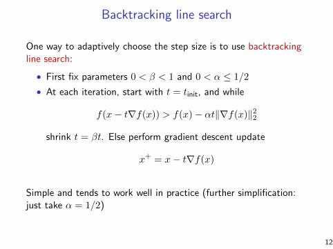
Backtracking line search

One way to adaptively choose the step size is to use backtrackingline search:

• First fix parameters 0 < β < 1 and 0 < α ≤ 1/2

• At each iteration, start with t = tinit, and while

f(x− t∇f(x)) > f(x)− αt‖∇f(x)‖22

shrink t = βt. Else perform gradient descent update

x+ = x− t∇f(x)

Simple and tends to work well in practice (further simplification:just take α = 1/2)

12

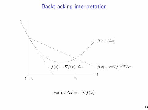
Backtracking interpretation9.2 Descent methods 465

t

f(x + t∆x)

t = 0 t0

f(x) + αt∇f(x)T ∆xf(x) + t∇f(x)T ∆x

Figure 9.1 Backtracking line search. The curve shows f , restricted to the lineover which we search. The lower dashed line shows the linear extrapolationof f , and the upper dashed line has a slope a factor of α smaller. Thebacktracking condition is that f lies below the upper dashed line, i.e., 0 ≤t ≤ t0.

The line search is called backtracking because it starts with unit step size andthen reduces it by the factor β until the stopping condition f(x + t∆x) ≤ f(x) +αt∇f(x)T ∆x holds. Since ∆x is a descent direction, we have ∇f(x)T ∆x < 0, sofor small enough t we have

f(x + t∆x) ≈ f(x) + t∇f(x)T ∆x < f(x) + αt∇f(x)T ∆x,

which shows that the backtracking line search eventually terminates. The constantα can be interpreted as the fraction of the decrease in f predicted by linear extrap-olation that we will accept. (The reason for requiring α to be smaller than 0.5 willbecome clear later.)

The backtracking condition is illustrated in figure 9.1. This figure suggests,and it can be shown, that the backtracking exit inequality f(x + t∆x) ≤ f(x) +αt∇f(x)T ∆x holds for t ≥ 0 in an interval (0, t0]. It follows that the backtrackingline search stops with a step length t that satisfies

t = 1, or t ∈ (βt0, t0].

The first case occurs when the step length t = 1 satisfies the backtracking condition,i.e., 1 ≤ t0. In particular, we can say that the step length obtained by backtrackingline search satisfies

t ≥ min{1,βt0}.

When dom f is not all of Rn, the condition f(x+ t∆x) ≤ f(x)+αt∇f(x)T ∆xin the backtracking line search must be interpreted carefully. By our conventionthat f is infinite outside its domain, the inequality implies that x + t∆x ∈ dom f .In a practical implementation, we first multiply t by β until x + t∆x ∈ dom f ;

For us ∆x = −∇f(x)

13

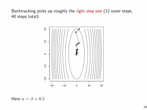
Backtracking picks up roughly the right step size (12 outer steps,40 steps total):

−20 −10 0 10 20

−20

−10

010

20 ●

●

●●●

●●●

●●●●

*

Here α = β = 0.5

14

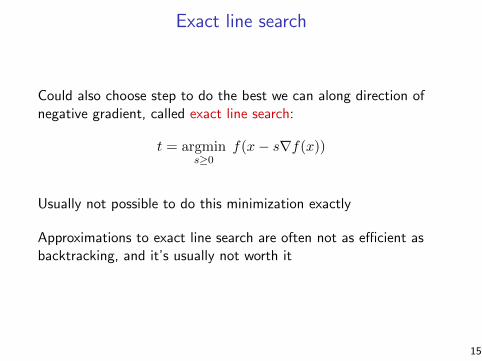
Exact line search

Could also choose step to do the best we can along direction ofnegative gradient, called exact line search:

t = argmins≥0

f(x− s∇f(x))

Usually not possible to do this minimization exactly

Approximations to exact line search are often not as efficient asbacktracking, and it’s usually not worth it

15

Convergence analysis

Assume that f convex and differentiable, with dom(f) = Rn, andadditionally

‖∇f(x)−∇f(y)‖2 ≤ L‖x− y‖2 for any x, y

I.e., ∇f is Lipschitz continuous with constant L > 0

Theorem: Gradient descent with fixed step size t ≤ 1/L satisfies

f(x(k))− f? ≤ ‖x(0) − x?‖22

2tk

We say gradient descent has convergence rate O(1/k)

I.e., to get f(x(k))− f? ≤ ε, we need O(1/ε) iterations

16

Proof

Key steps:

• ∇f Lipschitz with constant L ⇒

f(y) ≤ f(x) +∇f(x)T (y − x) +L

2‖y − x‖22 all x, y

• Plugging in y = x+ = x− t∇f(x),

f(x+) ≤ f(x)−(

1− Lt

2

)t‖∇f(x)‖22

• Taking 0 < t ≤ 1/L, and using convexity of f ,

f(x+) ≤ f? +∇f(x)T (x− x?)− t

2‖∇f(x)‖22

= f? +1

2t

(‖x− x?‖22 − ‖x+ − x?‖22

)

17

• Summing over iterations:

k∑

i=1

(f(x(i))− f?) ≤ 1

2t

(‖x(0) − x?‖22 − ‖x(k) − x?‖22

)

≤ 1

2t‖x(0) − x?‖22

• Since f(x(k)) is nonincreasing,

f(x(k))− f? ≤ 1

k

k∑

i=1

(f(x(i))− f?

)≤ ‖x

(0) − x?‖222tk

18

Convergence analysis for backtracking

Same assumptions, f is convex and differentiable, dom(f) = Rn,and ∇f is Lipschitz continuous with constant L > 0

Same rate for a step size chosen by backtracking search

Theorem: Gradient descent with backtracking line search satis-fies

f(x(k))− f? ≤ ‖x(0) − x?‖222tmink

where tmin = min{1, β/L}

If β is not too small, then we don’t lose much compared to fixedstep size (β/L vs 1/L)

19

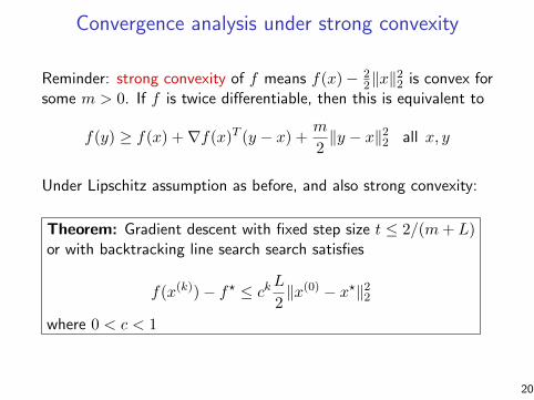
Convergence analysis under strong convexity

Reminder: strong convexity of f means f(x)− 22‖x‖22 is convex for

some m > 0. If f is twice differentiable, then this is equivalent to

f(y) ≥ f(x) +∇f(x)T (y − x) +m

2‖y − x‖22 all x, y

Under Lipschitz assumption as before, and also strong convexity:

Theorem: Gradient descent with fixed step size t ≤ 2/(m+ L)or with backtracking line search search satisfies

f(x(k))− f? ≤ ckL2‖x(0) − x?‖22

where 0 < c < 1

20

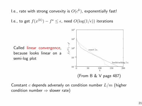
I.e., rate with strong convexity is O(ck), exponentially fast!

I.e., to get f(x(k))− f? ≤ ε, need O(log(1/ε)) iterations

Called linear convergence,because looks linear on asemi-log plot

9.3 Gradient descent method 473

kf(x

(k))−

p⋆

exact l.s.

backtracking l.s.

0 50 100 150 20010−4

10−2

100

102

104

Figure 9.6 Error f(x(k))−p⋆ versus iteration k for the gradient method withbacktracking and exact line search, for a problem in R100.

These experiments suggest that the effect of the backtracking parameters on theconvergence is not large, no more than a factor of two or so.

Gradient method and condition number

Our last experiment will illustrate the importance of the condition number of∇2f(x) (or the sublevel sets) on the rate of convergence of the gradient method.We start with the function given by (9.21), but replace the variable x by x = T x̄,where

T = diag((1, γ1/n, γ2/n, . . . , γ(n−1)/n)),

i.e., we minimize

f̄(x̄) = cT T x̄ −m!

i=1

log(bi − aTi T x̄). (9.22)

This gives us a family of optimization problems, indexed by γ, which affects theproblem condition number.

Figure 9.7 shows the number of iterations required to achieve f̄(x̄(k))−p̄⋆ < 10−5

as a function of γ, using a backtracking line search with α = 0.3 and β = 0.7. Thisplot shows that for diagonal scaling as small as 10 : 1 (i.e., γ = 10), the number ofiterations grows to more than a thousand; for a diagonal scaling of 20 or more, thegradient method slows to essentially useless.

The condition number of the Hessian ∇2f̄(x̄⋆) at the optimum is shown infigure 9.8. For large and small γ, the condition number increases roughly asmax{γ2, 1/γ2}, in a very similar way as the number of iterations depends on γ.This shows again that the relation between conditioning and convergence speed isa real phenomenon, and not just an artifact of our analysis.

(From B & V page 487)

Constant c depends adversely on condition number L/m (highercondition number ⇒ slower rate)

21

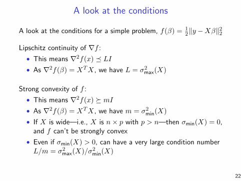
A look at the conditions

A look at the conditions for a simple problem, f(β) = 12‖y−Xβ‖22

Lipschitz continuity of ∇f :

• This means ∇2f(x) � LI• As ∇2f(β) = XTX, we have L = σ2max(X)

Strong convexity of f :

• This means ∇2f(x) � mI• As ∇2f(β) = XTX, we have m = σ2min(X)

• If X is wide—i.e., X is n× p with p > n—then σmin(X) = 0,and f can’t be strongly convex

• Even if σmin(X) > 0, can have a very large condition numberL/m = σ2max(X)/σ2min(X)

22

A function f having Lipschitz gradient and being strongly convexsatisfies:

mI � ∇2f(x) � LI for all x ∈ Rn,

for constants L > m > 0

Think of f being sandwiched between two quadratics

May seem like a strong condition to hold globally (for all x ∈ Rn).But a careful look at the proofs shows that we only need Lipschitzgradients/strong convexity over the sublevel set

S = {x : f(x) ≤ f(x(0))}

This is less restrictive (especially if S is compact)

23

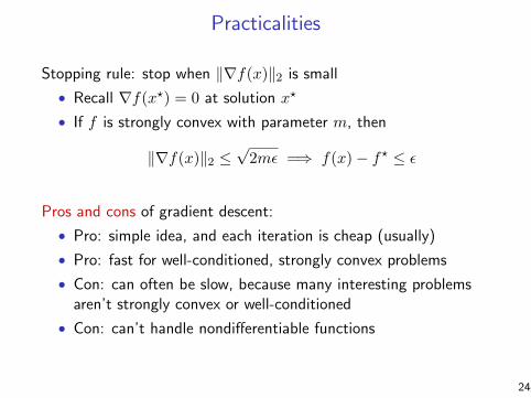
Practicalities

Stopping rule: stop when ‖∇f(x)‖2 is small

• Recall ∇f(x?) = 0 at solution x?

• If f is strongly convex with parameter m, then

‖∇f(x)‖2 ≤√

2mε =⇒ f(x)− f? ≤ ε

Pros and cons of gradient descent:

• Pro: simple idea, and each iteration is cheap (usually)

• Pro: fast for well-conditioned, strongly convex problems

• Con: can often be slow, because many interesting problemsaren’t strongly convex or well-conditioned

• Con: can’t handle nondifferentiable functions

24

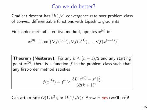
Can we do better?

Gradient descent has O(1/ε) convergence rate over problem classof convex, differentiable functions with Lipschitz gradients

First-order method: iterative method, updates x(k) in

x(0) + span{∇f(x(0)),∇f(x(1)), . . .∇f(x(k−1))}

Theorem (Nesterov): For any k ≤ (n− 1)/2 and any startingpoint x(0), there is a function f in the problem class such thatany first-order method satisfies

f(x(k))− f? ≥ 3L‖x(0) − x?‖2232(k + 1)2

Can attain rate O(1/k2), or O(1/√ε)? Answer: yes (we’ll see)!

25

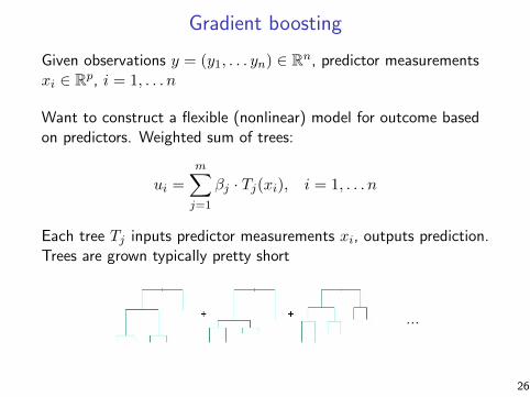
Gradient boosting

Given observations y = (y1, . . . yn) ∈ Rn, predictor measurementsxi ∈ Rp, i = 1, . . . n

Want to construct a flexible (nonlinear) model for outcome basedon predictors. Weighted sum of trees:

ui =

m∑

j=1

βj · Tj(xi), i = 1, . . . n

Each tree Tj inputs predictor measurements xi, outputs prediction.Trees are grown typically pretty short

...

26

Pick a loss function L that reflects setting; e.g., for continuous y,could take L(yi, ui) = (yi − ui)2

Want to solve

minβ

n∑

i=1

L(yi,

M∑

j=1

βj · Tj(xi))

Indexes all trees of a fixed size (e.g., depth = 5), so M is huge

Space is simply too big to optimize

Gradient boosting: basically a version of gradient descent that isforced to work with trees

First think of optimization as minu f(u), over predicted values u,subject to u coming from trees

27

Start with initial model, e.g., fit a single tree u(0) = T0. Repeat:

• Compute negative gradient d at latest prediction u(k−1),

di = −[∂L(yi, ui)

∂ui

] ∣∣∣∣ui=u

(k−1)i

, i = 1, . . . n

• Find a tree Tk that is close to a, i.e., according to

mintrees T

n∑

i=1

(di − T (xi))2

Not hard to (approximately) solve for a single tree

• Compute step size αk, and update our prediction:

u(k) = u(k−1) + αk · Tk

Note: predictions are weighted sums of trees, as desired

28

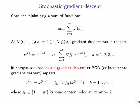
Stochastic gradient descent

Consider minimizing a sum of functions

minx

m∑

i=1

fi(x)

As ∇∑mi=1 fi(x) =

∑mi=1∇fi(x), gradient descent would repeat:

x(k) = x(k−1) − tk ·m∑

i=1

∇fi(x(k−1)), k = 1, 2, 3, . . .

In comparison, stochastic gradient descent or SGD (or incrementalgradient descent) repeats:

x(k) = x(k−1) − tk · ∇fik(x(k−1)), k = 1, 2, 3, . . .

where ik ∈ {1, . . .m} is some chosen index at iteration k

29

Two rules for choosing index ik at iteration k:

• Cyclic rule: choose ik = 1, 2, . . .m, 1, 2, . . .m, . . .

• Randomized rule: choose ik ∈ {1, . . .m} uniformly at random

Randomized rule is more common in practice

What’s the difference between stochastic and usual (called batch)methods? Computationally, m stochastic steps ≈ one batch step.But what about progress?

• Cyclic rule, m steps: x(k+m) = x(k) − t∑mi=1∇fi(x(k+i−1))

• Batch method, one step: x(k+1) = x(k) − t∑mi=1∇fi(x(k))

• Difference in direction is∑m

i=1[∇fi(x(k+i−1))−∇fi(x(k))]So SGD should converge if each ∇fi(x) doesn’t vary wildly with x

Rule of thumb: SGD thrives far from optimum, struggles close tooptimum ... (we’ll revisit in just a few lectures)

30

References and further reading

• D. Bertsekas (2010), “Incremental gradient, subgradient, andproximal methods for convex optimization: a survey”

• S. Boyd and L. Vandenberghe (2004), “Convex optimization”,Chapter 9

• T. Hastie, R. Tibshirani and J. Friedman (2009), “Theelements of statistical learning”, Chapters 10 and 16

• Y. Nesterov (1998), “Introductory lectures on convexoptimization: a basic course”, Chapter 2

• L. Vandenberghe, Lecture notes for EE 236C, UCLA, Spring2011-2012

31