Embed Size (px)
Citation preview

SPREADSHEET 1
Published by:
DEPARTMENT OF EDUCATION
GRADE 9
DESIGN AND TECHNOLOGY COMPUTING
UNIT 4
UNIT 4
FLEXIBLE OPEN AND DISTANCE EDUCATION PRIVATE MAIL BAG, P.O. WAIGANI, NCD FOR DEPARTMENT OF EDUCATION PAPUA NEW GUINEA


GR 9 D&T-COMPUTING U4 1 TITLE
Topic 1: Spreadsheet
Topic 2: Creating a Sample Worksheet
Topic 3: Making Simple Calculations
Topic 4: Doing More with Spreadsheet
GRADE 9 DESIGN AND TECHNOLOGY-COMPUTING
UNIT 4
SPREADSHEET 1

GR 9 D&T– COMPUTING U4 2 ACKNOWLEDGEMENT
Written and Compiled by Maria Imelda Somtragool. First Published in 2017 by Flexible Open and Distance Education, Papua New Guinea Printed by Flexible Open and Distance Education ISBN: 978-9980-89-649-0 National Library Services of Papua New Guinea
Acknowledgments
We acknowledge the contributions of all Secondary Teachers who in one way or another helped to develop this Course.
Our profound gratitude goes to the former Principal of FODE, Mr. Demas Tongogo for leading FODE team towards this great achievement. Special thanks to the FODE IT Edit Team and SRC Members who played an active role in critiquing and editing to ensure quality control for this Course.
We also acknowledge the professional guidance provided by the Curriculum Assessment Division throughout the process of writing especially to the late Mr. Tobias Gena.
The development of this book was co-funded by GoPNG and World Bank.
DIANA TEIT AKIS
PRINCIPAL
The development of this book was co-funded by GoPNG and World Bank.
DEMAS TONGOGO
PRINCIPAL

GR 9 D&T– COMPUTING U4 3 SECRETARY’S MESSAGE
SECRETARY’S MESSAGE Achieving a better future by individual students and their families, communities or the nation as a whole, depends on the kind of curriculum and the way it is delivered. This course is a part of the new Flexible, Open and Distance Education curriculum. The learning outcomes are student-centred and allows for them to be demonstrated and assessed. It maintains the rationale, goals, aims and principles of the national curriculum and identifies the knowledge, skills, attitudes and values that students should achieve. This is a provision by Flexible, Open and Distance Education as an alternative pathway of formal education. The course promotes Papua New Guinea values and beliefs which are found in our Constitution, Government Policies and Reports. It is developed in line with the National Education Plan (2005 -2014) and addresses an increase in the number of school leavers affected by the lack of access into secondary and higher educational institutions. Flexible, Open and Distance Education curriculum is guided by the Department of Education’s Mission which is fivefold: To facilitate and promote the integral development of every individual To develop and encourage an education system satisfies the requirements of Papua New Guinea and its people To establish, preserve and improve standards of education throughout Papua New Guinea To make the benefits of such education available as widely as possible to all of the people To make the education accessible to the poor and physically, mentally and socially handicapped as well as to those who are educationally disadvantaged. The college is enhanced to provide alternative and comparable pathways for students and adults to complete their education through a one system, many pathways and same outcomes. It is our vision that Papua New Guineans’ harness all appropriate and affordable technologies to pursue this program. I commend all those teachers, curriculum writers, university lecturers and many others who have contributed in developing this course.
UKE KOMBRA, PhD Secretary for Education
GR 9 D&T– COMPUTING U4 4 CONTENTS
TABLE OF CONTENTS
ACKNOWLEDGEMENT………………………………………………………………. 2
SECRETARY’S MESSAGE……………………………….………………….. ……….. 3
TABLE OF CONTENTS ………………………………………………………………. 4
UNIT INTRODUCTION ………………………………………………………………. 5
STUDY GUIDE ………………………………………………………………………… 6
TOPIC 1: SPREADSHEET
Lesson 1 The Spreadsheet and Its Purpose ………………. 9
Lesson 2 Planning the Content of Spreadsheet ………….. 17
Lesson 3 Ethical Use of Files and Data ……………….. 22
Lesson 4 Exploring the Excel Window ………………… 27
Lesson 5 Moving Around in the Workbook …………… 34
Lesson 6 Saving and Exiting Excel ……………………. 43
Answers to Practical Exercises 1 – 6 …….………………….. 51
TOPIC 2: CREATING A SAMPLE WORKSHEET
Lesson 7 Setting Up Rows and Columns……………… 55
Lesson 8 Entering Data and Formula………………….. 65
Lesson 9 Adding and Deleting Rows and Columns …….. 74
Lesson 10 Editing Data…………………………………….. 89
Lesson 11 Setting Up Cell Attributes……………………… 101
Lesson 12 Sorting Data…………………………………….. 111
Answers to Practical Exercises 7 – 12 .…………………..….. 118
TOPIC 3: MAKING SIMPLE CALCULATIONS
Lesson 13 Adding Numbers in Various Cells…………… 123
Lesson 14 Subtracting Numbers in Various Cells………. 132
Lesson 15 Multiplying Numbers in Various Cells………. 137
Lesson 16 Dividing Two Numbers………………………. 143
Lesson 17 Using Auto Sum………………………………… 148
Lesson 18 Copying Data or Formula…………………… 157
Answers to Practical Exercises 13 – 18 .……………………. 167
TOPIC 4: DOING MORE WITH SPREADSHEET
Lesson 19 Creating a More Complex or Unusual Formula…… 173
Lesson 20 Formatting a Worksheet……………………………… 181
Lesson 21 Using Print Preview…………………………………… 190
Lesson 22 Printing a Worksheet………………………………….. 195
Lesson 23 Creating a Graph with Chart Wizard………………… 207
Lesson 24 Incorporate Graphs in Word Processing…………… 218
Answers to Practical Exercises 19 – 24…………………………….. 224
Glossary ………………………………………………………………………….……… 229
GR 9 D&T– COMPUTING U4 5 UNIT INTRODUCTION
Topic 1: Spreadsheet
Topic 2: Creating a Sample Worksheet
Topic 3: Making Simple Calculations
Topic 4: Doing More with Spreadsheet
UNIT INTRODUCTION
Unit 4 is Spreadsheet 1 where you will learn about the basic concepts of Spreadsheet. The Unit consists of the following four Topics:
By the end of this Unit you will have gained the skills and proficiency in the use of Spreadsheet programs, demonstrate skills required for Spreadsheet, use design process to produce solutions involving Spreadsheet and demonstrate ethical values on computer use like sharing files on one computer.

GR 9 D&T– COMPUTING U4 6 STUDY GUIDE
CHECK YOUR ANSWERS AT THE END OF TOPIC 1.
STUDY GUIDE
Below are steps to guide you in your course study. Step 1: Read each lesson in the Unit Book carefully. In most cases,
reading through a lesson once is not enough. It helps to read something over several times until you understand it. You are not expected to memorise the information in the Unit Book. You should use it as a reference and to learn from the examples given to illustrate important points.
Step 2: After reading the summary of the lesson, start doing the Practice Exercise. You must do only one practice exercise at a time. Then mark it according to the following instruction.
Step 3: After marking your answers, go back to the lesson and correct any mistakes you may have made. Then move on to the next lesson.
Step 4: After completing all the Practice Exercises, do Assignment 4. Step 5: Now send the completed Assignment booklet to FODE for
marking. Be honest with yourself when you are doing and marking your Practice Exercises as well as completing your Assignment Booklets. This Unit has a separate assignment booklet for you to use. The information at the end of the last lesson in every Topic will let you know what to do with the assignment exercises. Whenever you need help and advice, contact your tutor or your Provincial Coordinator for assistance. If you are in the NCD or Central Province, we are available on Mondays to Fridays. You can call in anytime between 8 a.m. and 4 p.m. We would be glad to help you. The following icons are the symbols used in this book to indicate the parts of your lessons. The following are the icons and their respective meanings.
We hope you enjoy learning this course. All the best! Your Teacher Information Technology Department FODE

GR 9 D&T– COMPUTING U4 7 TOPIC TITLE
TOPIC 1
INTRODUCTION TO SPREADSHEET
Lesson 1: The Spreadsheet and Its
Purpose
Lesson 2: Planning the Content of Spreadsheet
Lesson 3: Ethical Use of Files and Data
Lesson 4: Exploring the Excel Window
Lesson 5: Moving around the Workbook
Lesson 6: Saving and Exiting Excel

GR 9 D&T– COMPUTING U4 8 TOPIC INTRODUCTION
TOPIC 1: SPREADSHEET
___________________________________________________________________
In this topic you will learn about the basic concepts of a Spreadsheet. The Topic is designed to familiarise you with Spreadsheet. It aims to give you a basic understanding of facts and concepts necessary to have a head start in the study of computing.
Spreadsheet is more popular than ever today. It is a cornerstone of what people who like to use big words call as "Administrative Support Systems". Even a simple Spreadsheet gives a person enormous power to keep track of how money and information flows through a company, or to rapidly try out several values (for a product price or a test curve, for example) and see the result of each one.
In this topic you will study about the following:
Lesson 1 is the introduction of Spreadsheet and its purpose. You will learn about the definition of Spreadsheet and identify the purpose of Spreadsheet.
Lesson 2 is planning the content of the Spreadsheet. You will learn how to identify the parts of and plan a Spreadsheet.
Lesson 3 is about the ethical use of files and data. You will learn the definition and importance of ethical use of files and data.
Lesson 4 is exploring the Excel Window. You will explore the Excel Window, identify and locate its different parts.
Lesson 5 is about moving around in a Workbook. You will learn about the meaning and importance of a workbook then explore and use certain keys to move around it.
Lesson 6 explains saving and exiting Excel. You will learn about the definition of saving and how to save a workbook to different locations and exit an Excel workbook.

GR 9 D&T– COMPUTING U4 9 TOPIC 1 LESSON 1
Lesson 1: The Spreadsheet and Its Purpose ___________________________________________________________________
The Spreadsheet Spreadsheet is the application that launched the personal computer into the business world. The very first Spreadsheet Program, VisiCalc, was created for the Apple II line of computers and was an immediate success. Lotus was the first company to bring the Spreadsheet to the IBM PC compatible with Lotus 1-2-3. Other vendors quickly followed with their own versions of the application. As you progress in the course, you will see different pictures of different kinds of Spreadsheet. What is a Spreadsheet? A Spreadsheet provides way to set up relationships between numbers. A Spreadsheet can make graphs, do arithmetic and create really good-looking tables, most of which is just colourful stuff. The heart and soul of a Spreadsheet is its ability to let you set up relationships between sets of numbers and then play with the numbers to see what happens.
Some examples of how Spreadsheet can be useful include::
Interest earned is 4% of the current balance per year
The final car price is the dealer price + cost for extras + 10% commission
My cheque book balance is the amount of the initial deposit + all the deposits since then - all the withdrawals for the same period
By setting up correct relationships between the different values, we give ourselves the ability to "play" with the actual numbers to see what happens.
The Purposes of Spreadsheet The Spreadsheet has evolved to be a very useful tool to mankind. The following items below are the different purposes of Spreadsheet.
Spreadsheet holds and stores data.
Welcome to Lesson 1 of Unit 4. Unit 4 starts with the brief history and introduction of Spreadsheet. In this lesson you will learn about the definition and purpose of Spreadsheet.
Your Aims:
state the definition of a Spreadsheet
identify the purpose of Spreadsheet
trace the history of Spreadsheet
GR 9 D&T– COMPUTING U4 10 TOPIC 1 LESSON 1
Commonly used in the business and scientific fields, it can be set up in a thousand ways using rows and columns.
A Spreadsheet provides structure and organization of data and often makes calculations, easier.
It deals with any problems that involve a lot of numbers, many of which are dependent on each other or are likely to change as other values change.
Spreadsheet can handle anything you might need to graph, since all Spreadsheet have the ability to produce graphs and charts.
You can compute any problem where you need to play with numbers in order to find an "optimal" solution.
In some industries, Spreadsheet programs are often used heavily in the financial sector where keeping track of numerical data is extremely important.
Brief History of Spreadsheet Let us take a quick look at history and see how Spreadsheet came into existence. The VisiCalc VisiCalc, short for ―Visible Calculator,‖ was the first Spreadsheet programme and the first fully functional computer application to ran on personal computers.
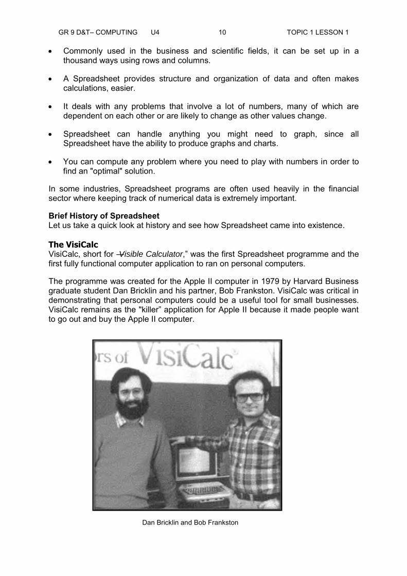
The programme was created for the Apple II computer in 1979 by Harvard Business graduate student Dan Bricklin and his partner, Bob Frankston. VisiCalc was critical in demonstrating that personal computers could be a useful tool for small businesses. VisiCalc remains as the "killer‖ application for Apple II because it made people want to go out and buy the Apple II computer.
Dan Bricklin and Bob Frankston
GR 9 D&T– COMPUTING U4 11 TOPIC 1 LESSON 1
Prior to the VisiCalc invention, computers could only run a few games and BASIC, a computer programming language. It was originally called Calculedger. The VisiCalc Spreadsheet software was a cross between a calculator and ledger. It was capable of calculating financial projections and complex ―what if‖ scenarios, using mathematical relationships between numbers.
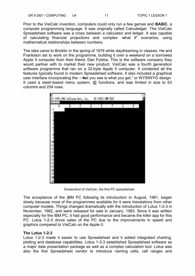
The idea came to Bricklin in the spring of 1978 while daydreaming in classes. He and Frankston set to work on the programme, building it over a weekend on a borrowed Apple II computer from their friend, Dan Fylstra. This is the software company they would partner with to market their new product. VisiCalc was a fourth generation software programme that ran on a 32-byte Apple II computer. It contained all the features typically found in modern Spreadsheet software. It also included a graphical user interface incorporating the ―what you see is what you get,‖ or WYSIWYG design. It used a slash-based menu system, @ functions, and was limited in size to 63 columns and 254 rows.
Screenshot of VisiCalc, the first PC spreadsheet.
The acceptance of the IBM PC following its introduction in August, 1981, began slowly because most of the programmes available for it were translations from other computer models. Things changed dramatically with the introduction of Lotus 1-2-3 in November, 1982, and were released for sale in January, 1983. Since it was written especially for the IBM PC, it had good performance and became the killer app for this PC. Lotus 1-2-3 drove sales of the PC due to the improvements in speed and graphics compared to VisiCalc on the Apple II.
The Lotus 1-2-3 Lotus 1-2-3 made it easier to use Spreadsheet and it added integrated charting, plotting and database capabilities. Lotus 1-2-3 established Spreadsheet software as a major data presentation package as well as a complex calculation tool. Lotus was also the first Spreadsheet vendor to introduce naming cells, cell ranges and
GR 9 D&T– COMPUTING U4 12 TOPIC 1 LESSON 1
For creating Spreadsheet macros, Kapor was the VisiCalc product manager at Personal Software for about six months in 1980. He also designed and programmed Visiplot/Visitrend which he sold to Personal Software (VisiCorp)for $1 million.
Part of that money along with funds from venture capitalist Ben Rosen was used to start Lotus Development Corporation in 1982. Kapor co-founded Lotus Development Corporation with Jonathan Sachs. Before he co-founded Lotus, Kapor disclosed and offered Personal Software (VisiCorp) his initial Lotus program. VisiCorp executives declined the offer because Lotus 1-2-3's functionality was "too limited". Lotus 1-2-3 is still one of the all-time best selling application software packages in the world.
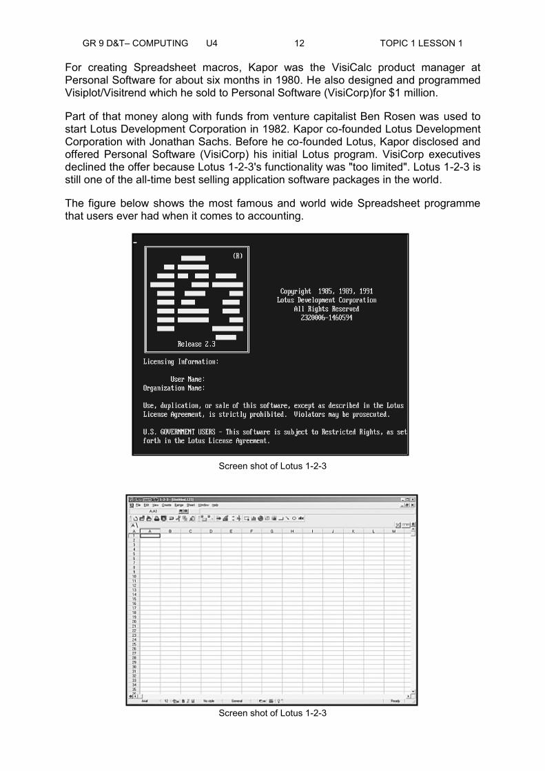
The figure below shows the most famous and world wide Spreadsheet programme that users ever had when it comes to accounting.
Screen shot of Lotus 1-2-3
Screen shot of Lotus 1-2-3

GR 9 D&T– COMPUTING U4 13 TOPIC 1 LESSON 1
The Microsoft Excel The next milestone in Spreadsheet was by the Microsoft Excel. Excel was originally written for the 512K Apple Macintosh in 1984-1985. Excel was one of the first spreadsheets to use a graphical user interface with pull down menus and a point and click capability using a pointing device such as a mouse. Since Excel used a graphical user interface it was easier for most people to use than the command line interface that most PC-DOS spreadsheet products relied on. Many people bought Apple Macintoshes so that they could use Bill Gates' Excel spreadsheet program.
By the late 1980s many companies had introduced spreadsheet products. Spreadsheet products and the spreadsheet software industry were maturing. Microsoft and Bill Gates had joined the battle for an innovative Excel spreadsheet. Lotus had acquired Software Arts and the rights to VisiCalc. Jim Manzi had become CEO at Lotus in April 1986 and in July 1986 Mitch Kapor resigned as Chairman of the Board. The spreadsheet entrepreneurs were moving on.
Spreadsheet has a wide range of uses. They can be used as a simple way to store numerical data or as an analytical tool making use of complex mathematical formulas, to solve complex numerical problems.
Activity 1: Answer the following questions.
A. Complete the following questions by providing your answers in the space provided. 1. Define Spreadsheet. ______________________________________________________________
______________________________________________________________
______________________________________________________________
______________________________________________________________
2. List down five (5) purposes of Spreadsheet.
a. ______________________________________________________________
______________________________________________________________
b. ______________________________________________________________
______________________________________________________________
c. ______________________________________________________________
______________________________________________________________

GR 9 D&T– COMPUTING U4 14 TOPIC 1 LESSON 1
d. ______________________________________________________________
______________________________________________________________
e. ______________________________________________________________
______________________________________________________________
B. Write the correct word or phrase in the blank. 1. VisiCalc is short for ―_________________,‖ was the first Spreadsheet
program and the first fully functional computer application to run on personal computers.
2. The program was created for the ______________ computer in 1979 by Harvard Business graduate student ______________ and his partner, Bob Frankston.
3. Originally called _____________, the VisiCalc Spreadsheet software was a cross between a calculator and ledger, capable of calculating financial projections and complex ―what if‖ scenarios, using mathematical relationships between numbers.
4. WYSIWYG means _____________________. 5. ________________is one of the all-time best selling application software
packages in the world.
Thank you for completing this activity. Now, you may go to the end of this lesson to check your answers. Make sure you do the necessary corrections before moving on to the next part of this lesson.
Summary You have come to the end of Lesson 1. In this lesson you learnt the basic understanding of facts and concepts necessary in the study of Spreadsheet.
NOW DO PRACTICE EXERCISE 1 ON THE NEXT PAGE.

GR 9 D&T– COMPUTING U4 15 TOPIC 1 LESSON 1
Practice Exercise: 1
___________________________________________________________________
A. Write T if the given statement is correct and F if it is incorrect.
1. Lotus was the first company to bring the Spreadsheet to the IBM PC compatible with Lotus 1-2-3. ________
2. Spreadsheet can be used as a simple way to store numerical data or as tool to analyse complex mathematical formulas. _________
3. Spreadsheet is a way to set up relationships between numbers. _________
4. Spreadsheet is commonly used in the business and scientific fields. A Spreadsheet can be set up in various ways using rows and columns. ________
5. VisiCalc is short for Visual Calculator. _________
6. All Spreadsheet programs have a graphing program built into them. _________
7. Spreadsheet is the solution for any problem that involves a lot of numbers. _________
8. Accountants and bankers are likely to use Spreadsheet daily. ________
9. Spreadsheet programs are often used heavily in some industries for their financial sector where keeping track of numerical data is extremely important. _________
10. Spreadsheet will make graphs, do arithmetic and create really good- looking pictures. __________
___________________________________________________________________
B. Choose the correct words from the box. Write the answers on the spaces provided.
numbers mathematical VisiCalc numerical
1. The very first Spreadsheet, ________________, was created for the Apple II line of computers.
2. Spreadsheet be used as a simple way to store ______________ data or as an analytical tool making use of complex _____________ formulas.
3. The heart and soul of a Spreadsheet is its ability to let you set up relationships between sets of __________.
___________________________________________________________________
CHECK YOUR WORK. ANSWERS ARE AT THE END OF TOPIC 1.

GR 9 D&T– COMPUTING U4 16 TOPIC 1 LESSON 1
Answers to Activity 1
A. 1. The definition of Spreadsheet
A Spreadsheet is a way to set up relationships between numbers. A Spreadsheet will make graphs, do arithmetic and create really good- looking tables.
2. Purposes of Spreadsheet: (Any of these 5 answers)
a. Spreadsheet holds and stores data.
b. Commonly used in the business and scientific fields. A Spreadsheet can be set up in various ways using rows and columns.
c. A Spreadsheet provides structure and organization for data and often makes calculations.
d. Any problem that involves a lot of numbers, many of which are dependent on each other or are likely to change.
e. Anything you might need to graph, since all Spreadsheet have a graphing program built into them.
f. Any problem where you need to play with numbers in order to find an "optimal" solution.
g. In some industries, Spreadsheet programs are often used heavily in the financial sector where keeping track of numerical data is extremely important.
h. Accountants and bankers are likely to use Spreadsheet every day.
B. 1. Visible Calculator
2. Apple II, Dan Bricklin
3. Calculedger
4. What you see is what you get.
5. Lotus 1 2 3

GR 9 D&T– COMPUTING U4 17 TOPIC 1 LESSON 2
Lesson 2: Planning the Content of Spreadsheet
___________________________________________________________________
Planning the Content of a Spreadsheet In Lesson 1 we discussed the purposes of a Spreadsheet. Now let us discuss the uses of Spreadsheet. A Spreadsheet can be used in the home and in business to do the following:
budget preparation
working trial balances
business modelling
sales forecasting
investment analysis
payroll
real estate management
taxes
investment proposals
Spreadsheet can be used for completing any data calculation involving numbers and text normally performed with pencil, paper, and calculator.
When dealing with a problem, you should try to develop a plan for handling it as early in the process as possible. A lot of additional work can be avoided by prior planning. Your end product will look better, and you will avoid unnecessary changes later on.
The steps in the planning process are:
Determining the purposes – The first step is to determine exactly what the purpose or goal of the worksheet is. In other words, what do you want it to do for you? What inputs will be necessary to provide to the worksheet? What outputs do you want the Spreadsheet to generate? Are printed reports needed to make the information provide useful?
Planning – The second step is to plan a blueprint for your worksheet on paper. This blueprint should maintain the same rectangular format presented by the screen you are using. It should include all screens that will have explanations to you or other users. Remember that you may use this Spreadsheet only once a year and may not remember the notes of your Spreadsheet
Welcome to Lesson 2 of Unit 4. In Lesson 1, you learned about the history, definition and purposes of Spreadsheet.
In this lesson you will plan the content of a Spreadsheet.
Your Aim:
critically plan the content of a Spreadsheet
GR 9 D&T– COMPUTING U4 18 TOPIC 1 LESSON 2
logic after such a long separation. You should also plan how you will manipulate your data.
Building and Testing- The third step is to build and test your spreadsheet. If you have planned everything properly, this should go smoothly. Testing the Spreadsheet involves making sure that it manipulates the data correctly. A lot of things can go wrong-for instance, a formula might reference an incorrect cell, or it might be entered incorrectly.
Documenting- The final step is to finish the documentation for using the spreadsheet. Some of this documentation is included within the spreadsheet itself, but a lot of other concepts may have to be covered to allow a user other than the spreadsheet’s author to operate it effectively. In addition, limitations on inputs and outputs must be communicated and if the worksheet is to be used as a template within an organization, its date of creation and its author’s name and telephone number must be provided.
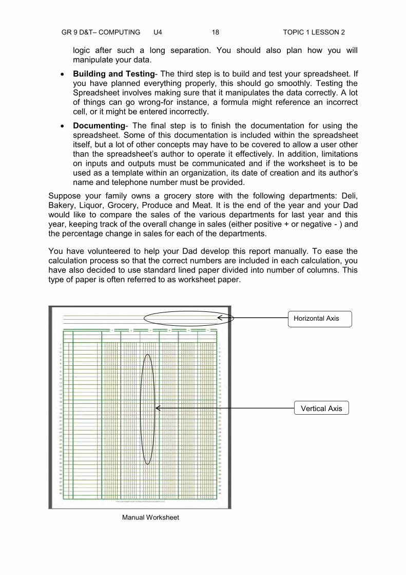
Suppose your family owns a grocery store with the following departments: Deli, Bakery, Liquor, Grocery, Produce and Meat. It is the end of the year and your Dad would like to compare the sales of the various departments for last year and this year, keeping track of the overall change in sales (either positive + or negative - ) and the percentage change in sales for each of the departments.
You have volunteered to help your Dad develop this report manually. To ease the calculation process so that the correct numbers are included in each calculation, you have also decided to use standard lined paper divided into number of columns. This type of paper is often referred to as worksheet paper.
Manual Worksheet
Horizontal Axis
Vertical Axis

GR 9 D&T– COMPUTING U4 19 TOPIC 1 LESSON 2
Apart from this worksheet paper, you need a pencil, an eraser, a ruler, and a calculator to make a manual Spreadsheet. In designing the report, you decide that the easiest way to present the data is to have the vertical axis and the horizontal axis.
Activity 1: Answer each question.
1. State the uses of spreadsheet in a business: a. _______________________
b.________________________ c.________________________
d. _______________________ e. _______________________
f. _______________________ g. _______________________
h. _______________________ i. ________________________
2. What are the five planning steps in preparing a Spreadsheet?
a. _______________________ b.________________________
c. _______________________
d.________________________ e.________________________
3. List down the materials you will need to make a manual Spreadsheet. a. _______________________ b. _______________________ c. ________________________
d. _______________________ e. _______________________
Thank you for completing this activity. Now, you may go to the end of this lesson to check your answers. Make sure you do the necessary corrections before moving on to the next part of this lesson. ___________________________________________________________________
Summary You have come to the end of Lesson 2. In this lesson you learnt the purposes of Spreadsheet and the planning process to make the Spreadsheet look better and also to avoid unnecessary changes later on. In addition to this, we looked at a standard lined paper divided
into number of columns referred to as the worksheet paper. ___________________________________________________________________
NOW DO PRACTICE EXERCISE 2 ON THE NEXT PAGE.

GR 9 D&T– COMPUTING U4 20 TOPIC 1 LESSON 2
Practice Exercise: 2
1. Complete the manual worksheet by entering it with the given data. The first one is done for you as an example.
The given data:
Department Last Year This Year
Deli 700 515
Bakery 1000 1100
Liquor 1200 1400
Grocery 2500 2900
Produce 950 1000
Meat 1500 1410
2. Comparative Sales Report for the last two years.
Department Last Year This Year
1 Deli 7 0 0 5 1 5
__________________________________________________________________
CHECK YOUR WORK. ANSWERS ARE AT THE END OF TOPIC 1.
Answers to Activity
1. The uses of Spreadsheet in a business
a. budget preparation b. working trial balances c. business modelling d. sales forecasting

GR 9 D&T– COMPUTING U4 21 TOPIC 1 LESSON 2
e. investment analysis
f. payroll
g. real estate management
h. taxes
i. investment proposals
2. Five planning steps in doing a Spreadsheet
a. Determining the purposes
b. Planning
c. Building
d. Testing
e. Documenting
3. The materials needed to make a manual Spreadsheet
a. pencil
b. paper
c. calculator
d. eraser
e. ruler
GR 9 D&T– COMPUTING U4 22 TOPIC 1 LESSON 3
Lesson 3: Ethical Use of Files and Data
___________________________________________________________________
Welcome to Lesson 3 of Unit 4. In Lesson 2, you learnt about the planning process and the purposes of Spreadsheet. In this lesson we will discuss the ethical issues on how institutions use the Spreadsheet, its complexity and potential risk and issues.
Your Aims:
___________________________________________________________________ The Ethical Use of Files and Data Many companies rely on Spreadsheet as a key component in their financial reporting and operational processes. However, it is clear that the flexibility of Spreadsheet has sometimes come at a cost.
Legal and Ethical Issues in Spreadsheet Microsoft Excel is frequently used to create Spreadsheet for sensitive legal and business documents such as business plans, contracts and financial information.
Because these documents can expose businesses to legal and ethical liability, it is important to incorporate ethical considerations into Spreadsheet design.
Background Spreadsheet typically have a wide range of complexity and usage. It is important to separate the complexity and usage issues, as the control requirements may be different for a complex Spreadsheet used by one person with specific expertise than for a Spreadsheet used and modified by many people. Whatever the situation, companies need to carefully evaluate if it is possible to implement adequate controls over the Spreadsheet supporting significant accounts and disclosures.
The use of Spreadsheet—and, more importantly, the lack of controls over Spreadsheet—has been a contributing factor in financial reporting errors at a number of companies.
The examples included here highlight the importance of understanding how Spreadsheet are used in a company’s financial reporting process and evaluating the controls over Spreadsheet as part of the company’s overall process.
How Institutions Use the Spreadsheet To assess how institutions like a school are using Spreadsheet, it is helpful to categorize both the uses and complexity of Spreadsheet.
The uses of information contained in Spreadsheet can be grouped into the following categories:
demonstrate an understanding of the ethical use of files and data
appreciate the ethical use of files and data
GR 9 D&T– COMPUTING U4 23 TOPIC 1 LESSON 3
1. Operational Spreadsheet used to facilitate tracking and monitoring of workflow to support operational processes. These may be used to monitor and control that financial transactions are captured accurately and completely.
2. Analytical/Management Information These may be used to make sure financial amounts are fair and sensible.
3. Financial Spreadsheet used to directly determine financial statement transaction amounts or balances that are populated into the general ledger and/or financial statements.
The complexity of Spreadsheet may be categorized in the following manner: 1. Low This is the Spreadsheet which serves as an electronic logging and information tracking system.
2. Moderate This is the Spreadsheet which performs simple calculations such as using formulas to total certain fields or calculate new values by multiplying two or more cells.
3. High This is the Spreadsheet which supports complex calculations, valuations and modelling tools. Potential Risks and Issues with Spreadsheet When evaluating the risk and significance of potential Spreadsheet issues, consider the following:
a. Complexity of the Spreadsheet and calculations.
b. Purpose and use of the Spreadsheet.
c. Number of Spreadsheet users.
d. Type of potential input, logic, and interface errors.
e. Size of the Spreadsheet.
f. Degree of understanding and documentation of the Spreadsheet requirements by the developer.
g. Uses of the Spreadsheet output.
h. Frequency and extent of changes and modifications to the Spreadsheet.
i. Development, developer (and training) and testing of the Spreadsheet before it is utilized.
GR 9 D&T– COMPUTING U4 24 TOPIC 1 LESSON 3
Activity 1: Answer each question.
1. Discuss and list briefly the legal and ethical issues in Spreadsheet. ______________________________________________________________
______________________________________________________________
______________________________________________________________
______________________________________________________________
2. State the nine (9) potential risks and issues with Spreadsheet. a. ____________________________________________________________
b. ____________________________________________________________
c. ____________________________________________________________
d. ____________________________________________________________
e. ____________________________________________________________
f. _____________________________________________________________
g. ____________________________________________________________
h. ____________________________________________________________
i. _____________________________________________________________
Thank you for completing this activity. Now, you may go to the end of this lesson to check your answers. Make sure you do the necessary corrections before moving on to the next part of this lesson.
Summary You have come to the end of Lesson 3. In this lesson you learnt and understand the ethical use of files and data, and appreciate the ethical use of files and data.
___________________________________________________________________
NOW DO PRACTICE EXERCISE 3 ON THE NEXT PAGE.

GR 9 D&T– COMPUTING U4 25 TOPIC 1 LESSON 3
Practice Exercise: 3
A. Write T if the statement is correct and write F if it is incorrect. 1. Many companies rely on Spreadsheet as a key component in their financial reporting and operational processes. ________
2. Microsoft Excel is frequently used to create Spreadsheet for sensitive legal and business documents such as business plans, contracts and financial information. _________
3. Spreadsheet typically has a wide range of complexity and usage. _________
4. As some companies have discovered, errors in relatively simple Spreadsheet can result in potential material misstatements in their financial results. ________
5. Spreadsheet is used and modified by many people. _________
6. Spreadsheet is used in a company’s financial reporting. _________
7. Spreadsheet is used to facilitate tracking and monitoring of workflow to support operational processes. _________
8. Spreadsheet serves as an electronic logging and information tracking system. ________
9. Moderate Spreadsheet can perform simple calculation. __________
10. Spreadsheet does not support complex calculations, valuations and modelling tools. __________
___________________________________________________________________
CHECK YOUR WORK. ANSWERS ARE AT THE END OF TOPIC 1.
Answers to Activity 1 1. The legal and ethical issues in Spreadsheet. Many companies rely on Spreadsheet as a key component in their financial reporting and operational processes. It is important that management identify where control breakdowns could lead to potential material misstatements and that controls for significant Spreadsheet be documented, evaluated and tested. Understanding how Spreadsheet are used and the adequacy of related controls is a critical part of management’s assessment of the effectiveness of its internal control over financial reporting.
2. Potential Risks and Issues with Spreadsheet
a. Complexity of the Spreadsheet and calculations.
GR 9 D&T– COMPUTING U4 26 TOPIC 1 LESSON 3
b. Purpose and use of the Spreadsheet.
c. Number of Spreadsheet users.
d. Type of potential input, logic, and interface errors.
e. Size of the Spreadsheet.
f. Degree of understanding and documentation of the Spreadsheet requirements by the developer.
g. Uses of the Spreadsheet output.
h. Frequency and extent of changes and modifications to the Spreadsheet.
i. Development, developer (and training) and testing of the Spreadsheet before it is utilized.
GR 9 D&T– COMPUTING U4 27 TOPIC 1 LESSON 4
Lesson 4: Exploring the Excel Window
__________________________________________________________________
Welcome to Lesson 4 of Unit 4. In Lesson 3, you learnt about the ethical issues about the use of Spreadsheet. In this lesson you will be able to define and identify the Excel window then differentiate and locate its parts.
___________________________________________________________________ The Microsoft Excel Microsoft Excel (MS Excel) 2010 is the newest version of Microsoft Office’s Spreadsheet program. It is a powerful spreadsheet program that allows you to organise and graph data, complete calculations, make decisions, develop reports, publish data on the Web, and access real time data from Web sites. Excel 2010 takes advantage of a new, results-oriented user interface to make powerful productivity tools easily accessible. If you are worried about capacity, Excel 2010 now accommodates 1 million rows and 16,000 columns. It also allows you to store, organise, and analyse information. It replaces the Microsoft Button menu from Excel 2007. The Excel 2010 interface is very similar to Excel 2007. But if you are new to Excel, it will take some time to learn to move around an Excel workbook. The picture on the right side is the MS Excel icon. Before we start, let us first define some of the terms that we will use in this lesson. You will see the diagram of Excel 2010 on the next page. 1. Quick Access Toolbar – is located above the Ribbon, and it lets you access common commands no matter which tabs you are on. By default, it shows the Save, Undo, and Repeat commands.
2. Ribbons – contain multiple tabs each with several groups of commands.
3. Formula Bar – displays information entered or being entered as you type-in the current or active cell. The contents of a cell can also be edited in the Formula Bar.
4. Name Box – shows the cell address of the current selection or active cell.
5. Active Cell (Cell Address) – is an intersection of a column and row. It is the selected cell and the location of what is being modified.
6. Sheet Tabs – separates workbooks into worksheets. It is a workbook by defaults to three worksheets. A workbook must contain at least one worksheet.
Your Aims:
identify the parts of an Excel window
differentiate the functions of each parts
locate the different parts of an Excel window

GR 9 D&T– COMPUTING U4 28 TOPIC 1 LESSON 4
7. Rows – are represented by numbers that appear on the left and then run down the Excel program window.
8. Columns – are represented by alphabetic characters across the top of the Excel screen.
9. Vertical Scroll Bar – located along the right edge of the Excel window is used to move up or down the spreadsheet.
10. Horizontal Scroll Bar – located at the bottom of the screen is used to move left or right across the spreadsheet.
Study the diagram below to familiarize yourself with the Microsoft Excel 2010 Environment.
How to Open an Excel Program Now that you know the terms used in Microsoft Excel, let us explore the Excel 2010 environment. The following steps will teach you how to open an Excel Program. Carefully follow each step. Be sure to have your computer ready.
1. Click the Start button.
2. Click All Programs.
1
2
The Microsoft Excel 2010 Environment
Active cell
Rows
Columns
Quick Access Toolbar Menu
Name Box
Formula Bar
Sheet Tabs
Vertical Scroll Bar
Horizontal Scroll Bar

GR 9 D&T– COMPUTING U4 29 TOPIC 1 LESSON 4
3. Click MS Office folder in the menu.
4. Click Microsoft Excel 2010 program icon.
The Functions of Excel Microsoft Excel serves a variety of functions. Study the different functions of the MS Excel. 1. The Ribbon The Ribbon contains multiple tabs, each with several groups of commands. You can add your own tabs that contain your favourite commands.
The Ribbon
3
4
GR 9 D&T– COMPUTING U4 30 TOPIC 1 LESSON 4
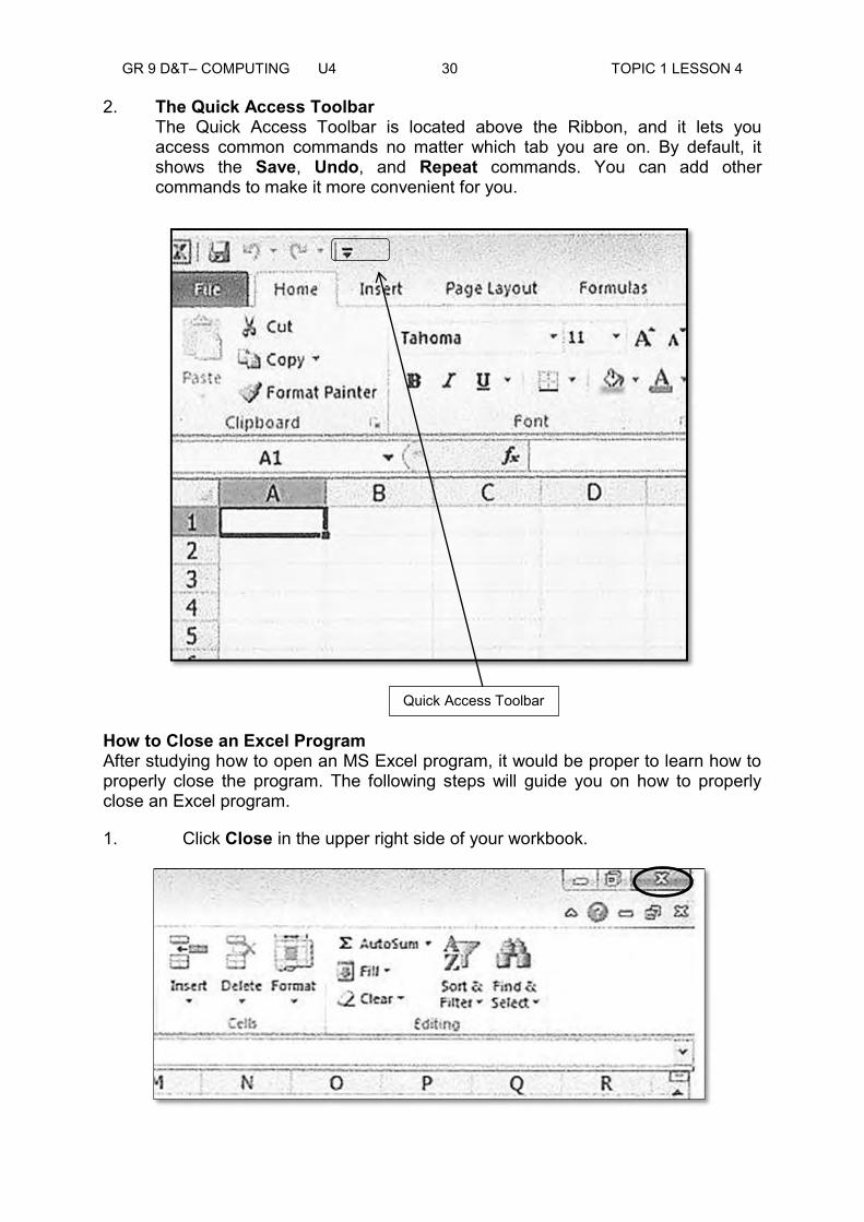
2. The Quick Access Toolbar The Quick Access Toolbar is located above the Ribbon, and it lets you access common commands no matter which tab you are on. By default, it shows the Save, Undo, and Repeat commands. You can add other commands to make it more convenient for you.
How to Close an Excel Program After studying how to open an MS Excel program, it would be proper to learn how to properly close the program. The following steps will guide you on how to properly close an Excel program.
1. Click Close in the upper right side of your workbook.
Quick Access Toolbar

GR 9 D&T– COMPUTING U4 32 TOPIC 1 LESSON 4
2. Click Don’t Save, if you are asked to save changes as book 1.
Activity 1: Follow the instructions below.
A. By using the Start Menu 1. Click the Start button.
2. See if you have the MS Excel Icon.
3. Click the File Tab.
4. Click Close , to close your workbook.
B. By using MS Excel Icon from the desktop
1. From the desktop, position your mouse on top of your MS Excel icon then double click the left button of your mouse.
2. Click Close , to close your workbook.

GR 9 D&T– COMPUTING U4 33 TOPIC 1 LESSON 4
C. By using MS Excel from the MS Office 2010 Menu Folder
1. Follow the steps you performed earlier in MS Excel on page 31.
2. Close your workbook.
Thank you for completing this activity. Make sure you do the necessary corrections to practice more the skills before moving on to the next part of this lesson.
___________________________________________________________________ Summary You have come to the end of Lesson 4. In this lesson, you have learnt some of the definitions of an Excel Window and to identify the parts of an Excel window. You have also learnt how to open and close an Excel workbook and some of the important parts of Excel.
NOW DO PRACTICE EXERCISE 4 ON THE NEXT PAGE.

GR 9 D&T– COMPUTING U4 34 TOPIC 1 LESSON 4
Practice Exercise: 4
___________________________________________________________________
A. Label the parts of the MS Excel Screen.
1. _________________________ 4. ________________________
2. ______________________ 5. _____________________ 3. _________________________ 6. ________________________
__________________________________________________________________________
B. Fill in the blanks with the word or phrase.
1. Worksheets contain numerical information presented in tabular row and _________format with text that labels the data. They can also contain graphics and charts.
2. Quick Access Toolbar is located above the_____________, and it lets you access common commands no matter which tabs you are on. By default, it shows the Save, Undo, and Repeat commands.
3. The Name Box shows the ___________of the current cell selection or active cell.
4. __________ is represented by numbers that appear on the left and then run down the Excel program window.
5. The Vertical Scroll Bar located along the right edge of the screen is used to move ______________or ______________ the spreadsheet program window.
___________________________________________________________________
1 2 3 4
5 6
CHECK YOUR WORK. ANSWERS ARE AT THE END OF TOPIC 1.

GR 9 D&T– COMPUTING U4 35 TOPIC 1 LESSON 5
Lesson 5: Moving Around in the Workbook
___________________________________________________________________
___________________________________________________________________ The Excel Worksheet A blank workbook is displayed when you open a new Excel document and is named Book 1. The workbook looks like a notebook and contains sheets, called worksheets. A new workbook contains three default worksheets. More worksheet can be added to it. Each sheet has a name displayed on a sheet tab at the bottom of the workbook. An array of cells is called a sheet or worksheet. Technically a worksheet is a single document inside a workbook but we often use the terms worksheet, Spreadsheet and workbook to mean the same things. Worksheets contain numerical information presented in tabular row and column format with text that labels the data. They can also contain graphics and charts.
A screenshot of MS Excel workbook
Welcome to Lesson 5 of Unit 4. In Lesson 4, you learned to identify, differentiate and locate the parts of an Excel window.
In this lesson you will get to know how to explore and move around the workbook.
Your Aims:
define the meaning of a workbook
explore the workbook
use certain keys to move around the workbook
Sheet tabs/Worksheet tabs
Book1- Title Bar
GR 9 D&T– COMPUTING U4 36 TOPIC 1 LESSON 5
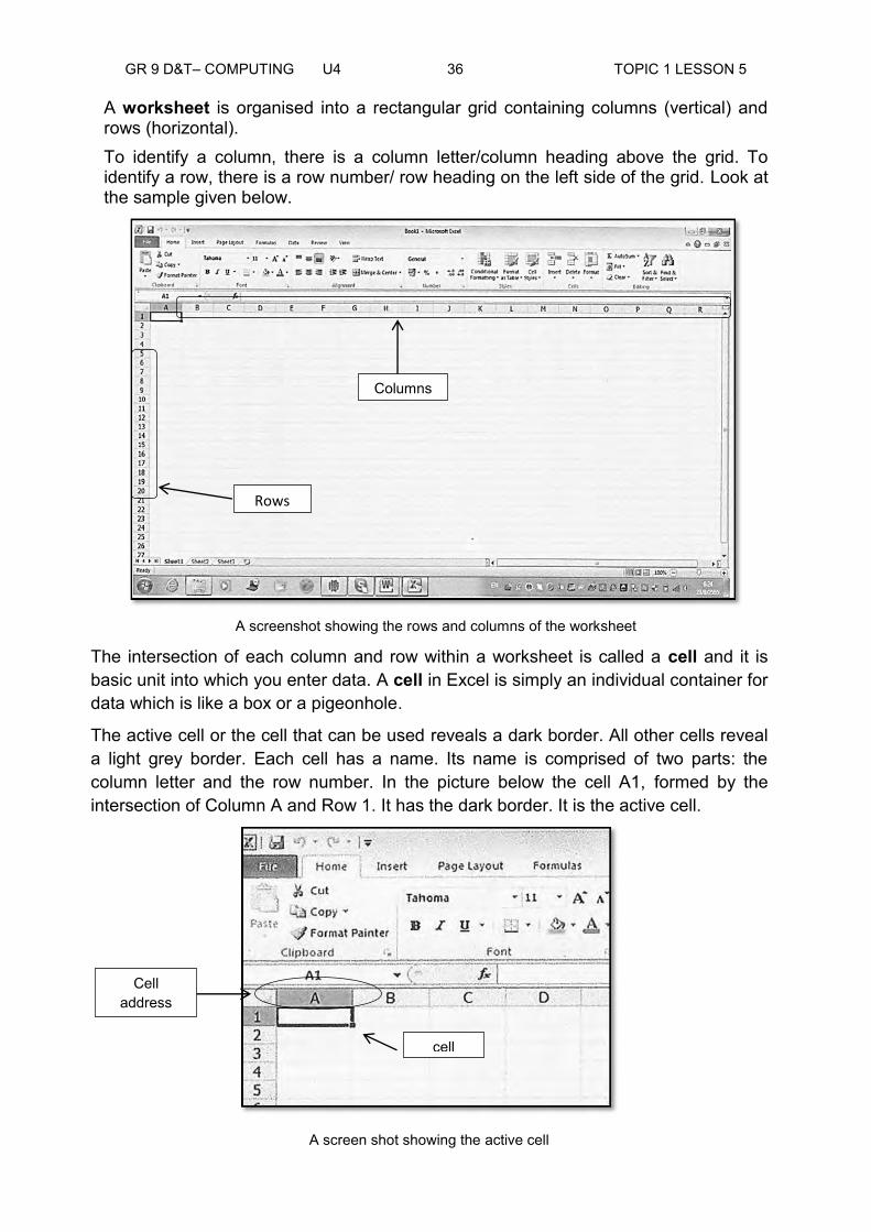
A worksheet is organised into a rectangular grid containing columns (vertical) and rows (horizontal). To identify a column, there is a column letter/column heading above the grid. To identify a row, there is a row number/ row heading on the left side of the grid. Look at the sample given below.
A screenshot showing the rows and columns of the worksheet
The intersection of each column and row within a worksheet is called a cell and it is basic unit into which you enter data. A cell in Excel is simply an individual container for data which is like a box or a pigeonhole.
The active cell or the cell that can be used reveals a dark border. All other cells reveal a light grey border. Each cell has a name. Its name is comprised of two parts: the column letter and the row number. In the picture below the cell A1, formed by the intersection of Column A and Row 1. It has the dark border. It is the active cell.
A screen shot showing the active cell
cell
Cell address
Rows
Columns

GR 9 D&T– COMPUTING U4 36 TOPIC 1 LESSON 5
Moving Around the Worksheet You can move around the Spreadsheet in several ways. 1. By Moving the Cell Pointer
To activate any cell, point to a cell with the mouse and click.
To move the pointer one cell to the left, right, up, or down, use the keyboard arrow keys.
2. By Scrolling Through the worksheet The vertical scroll bar located along the right edge of the screen is used to move up or down the Spreadsheet. The horizontal scroll bar located at the bottom of the screen is used to move left or right across the Spreadsheet.
A screenshot showing the scroll bars
The PageUp and PageDown keys on the keyboard are used to move the cursor up or down one screen at a time. Other keys that move the active cell are Home, which moves to the first column on the current row, and Ctrl+Home, which moves the cursor to the top left corner of the Spreadsheet or cell A1. 3. Moving between worksheets
As mentioned, each Workbook has three worksheets by default. These worksheets are represented by tabs - named Sheet1, Sheet2 and Sheet3 - that appear at the bottom of the Excel window.
Horizontal scroll bar
Vertical Scroll Bar
GR 9 D&T– COMPUTING U4 37 TOPIC 1 LESSON 5
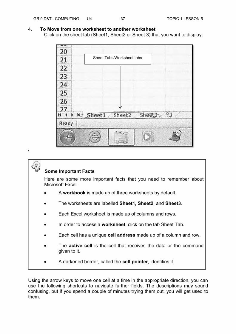
4. To Move from one worksheet to another worksheet Click on the sheet tab (Sheet1, Sheet2 or Sheet 3) that you want to display.
\
Some Important Facts Here are some more important facts that you need to remember about Microsoft Excel.
A workbook is made up of three worksheets by default.
The worksheets are labelled Sheet1, Sheet2, and Sheet3.
Each Excel worksheet is made up of columns and rows.
In order to access a worksheet, click on the tab Sheet Tab.
Each cell has a unique cell address made up of a column and row.
The active cell is the cell that receives the data or the command given to it.
A darkened border, called the cell pointer, identifies it.
Using the arrow keys to move one cell at a time in the appropriate direction, you can use the following shortcuts to navigate further fields. The descriptions may sound confusing, but if you spend a couple of minutes trying them out, you will get used to them.
Sheet Tabs/Worksheet tabs

GR 9 D&T– COMPUTING U4 38 TOPIC 1 LESSON 5
This next section will provide you some basic knowledge on short cut keys that you can use as you explore the Microsoft Excel Program.
Shortcut Actions Study the different ways on how to apply short cuts to different command in using the MS Excel. Think about the column the cursor is currently in. If the active cell
is in a range of cells holding data, the cursor jumps to the bottom most cell in that range. When the active cell is empty, the cursor jumps to the next cell down that contains the data.
If the active cell is in a range of cells holding data, the cursor
jumps to the cell topmost cell in that range. When the active cell is empty, the cursor jumps to the next cell that contains the data.
If the active cell is in a range of cells holding data, the cursor
jumps to the left most cell or right most cell in the range. When the active cell is empty, the cursor jumps to the next cell that contains data.
Displays the previous and next page in the worksheet Jumps to the very beginning of worksheet, i.e. cell A1 Jumps to the next/previous worksheet in the workbook Jumps to the end of the section of the worksheet that contains
data
Activity 1: Follow the instructions below to complete the activity.
A. Follow the steps below on how to move around in the workbook. 1. Click on each of the three (3) worksheets tabs-Sheet 1, Sheet 2 and Sheet 3 to practice moving from sheet to sheet in the workbook.
Ctrl-down arrow
Ctrl-up arrow
Ctrl-left arrow/Ctrl-right
arrow
Page-up/Page down
Ctrl-home
Ctrl-page down/ctrl-page up
Ctrl-end

GR 9 D&T– COMPUTING U4 39 TOPIC 1 LESSON 5
2. Scroll up and down the worksheet by using the Page Up (Pg Up) and Page Down (Pg Dn) key. Use the horizontal and vertical scrollbars to practice scrolling up, down, left and right in the worksheet.
3. Use the Shortcut keys to move your active cell to different locations according to the commands given in numbers 1 and 2. B. Make B3 your active cell and follow the instructions. 1. Ctrl-down arrow What will happen when you press this short cut keys in Excel?
Worksheet Tabs
Scroll Bars

GR 9 D&T– COMPUTING U4 40 TOPIC 1 LESSON 5
_____________________________________________________________
______________________________________________________________
______________________________________________________________
2. Ctrl-up arrow What happens when you press this short cut key in Excel? ______________________________________________________________
______________________________________________________________
______________________________________________________________
3. Ctrl-home What happens when you press this short cut key in Excel? ______________________________________________________________
______________________________________________________________
______________________________________________________________
Thank you for completing this activity. Make sure you do the necessary corrections to practice more the skills before moving on to the next part of this lesson.
___________________________________________________________________ Summary You have come to the end of Lesson 5. In this lesson, you have learnt how to move around the workbook. You explored and followed the steps on how to move around in Excel workbook. You also navigated certain short cut keys to move quickly through our workbook.
___________________________________________________________________
NOW DO PRACTICE EXERCISE 5 ON THE NEXT PAGE.
GR 9 D&T– COMPUTING U4 41 TOPIC 1 LESSON 5
Practice Exercise: 5 ___________________________________________________________________ A. Write T if the statement is True and F if it is false. 1. A workbook looks like a notebook and contains sheets, called worksheets. ________
2. A worksheet is organised into a rectangular grid containing columns (vertical) and rows (horizontal). _________
3. The intersection of each column and row within a worksheet is called a cell and it is the basic unit into which you enter data. ________
4. The worksheets are labelled Sheet1, Sheet2, and Sheet3.________
5. The horizontal scroll bar located along the right edge of the screen is used to move up or down the Spreadsheet. _________
___________________________________________________________________
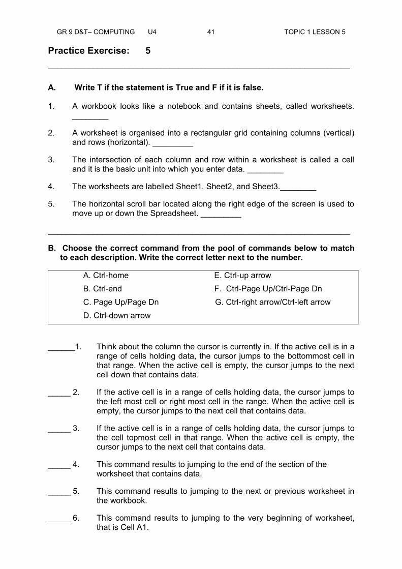
B. Choose the correct command from the pool of commands below to match to each description. Write the correct letter next to the number.
A. Ctrl-home E. Ctrl-up arrow B. Ctrl-end F. Ctrl-Page Up/Ctrl-Page Dn C. Page Up/Page Dn G. Ctrl-right arrow/Ctrl-left arrow D. Ctrl-down arrow
______1. Think about the column the cursor is currently in. If the active cell is in a range of cells holding data, the cursor jumps to the bottommost cell in that range. When the active cell is empty, the cursor jumps to the next cell down that contains data.
_____ 2. If the active cell is in a range of cells holding data, the cursor jumps to the left most cell or right most cell in the range. When the active cell is empty, the cursor jumps to the next cell that contains data.
_____ 3. If the active cell is in a range of cells holding data, the cursor jumps to the cell topmost cell in that range. When the active cell is empty, the cursor jumps to the next cell that contains data.
_____ 4. This command results to jumping to the end of the section of the worksheet that contains data.
_____ 5. This command results to jumping to the next or previous worksheet in the workbook.
_____ 6. This command results to jumping to the very beginning of worksheet, that is Cell A1.

GR 9 D&T– COMPUTING U4 42 TOPIC 1 LESSON 5
_____ 7. This command displays the previous and next page in the worksheet.
___________________________________________________________________
Answers to Activity
1. Ctrl-down arrow Think about the column the cursor is currently in. When the active cell is in a range of cells holding data, the cursor jumps to the bottommost cell in that range. When the active cell is empty, the cursor jumps to the next cell down that contains data.
2. Ctrl-up arrow If the active cell is in a range of cells holding data, the cursor jumps to the topmost cell in that range. When the active cell is empty, the cursor jumps to the next cell that contains data.
3. Ctrl-home Jumps to the very beginning of worksheet.
CHECK YOUR WORK. ANSWERS ARE AT THE END OF TOPIC 1.

GR 9 D&T– COMPUTING U4 43 TOPIC 1 LESSON 6
Lesson 6: Saving and Exiting Excel ___________________________________________________________________
____________________________________________________________________ Understanding File Terms
The File menu contains all the operations that we will discuss in this lesson. The following terms New, Open, Close, Save and Save As will assist you in understanding the lesson. Study them carefully.
New - a command that is used to create a new Workbook.
Open - a command that is used to open an existing file from a flash drive or hard drive of your computer.
Close - a command that is used to close a Spreadsheet.
Save As- a command that is used to save a new file for the first time or save an existing file with a different name.
Save- a command that is used to save a file that has had changes made to it. If you close the workbook without saving then any changes made will be lost.
Creating a Workbook A blank workbook is displayed when Microsoft Excel is first opened. You can type information or design a layout directly in this blank workbook. How to Create an Excel Workbook Creating an Excel Workbook is the next step in using the Microsoft Excel after learning how to open the program. The following steps and illustrations below will guide you on how to create a workbook.
1. Choose File from the menu bar.
2. Click New.
As you can see after clicking New, the Blank workbook from the Available Templates is highlighted with a yellow colour.
Your Aims:
define saving
save a workbook in different locations
exit Excel workbook
Welcome to Lesson 6 of Unit 1. In Lesson 5, you learned how to move around the workbook.
In this lesson you will define what Saving means in Excel, identify the differences between the commands: New, Open, Save and Save As and learn how to exit Excel.

GR 9 D&T– COMPUTING U4 44 TOPIC 1 LESSON 6
3. From the right hand side of the screen you can see the Create icon of the workbook, click create for a Blank Workbook.
Saving a Workbook Every workbook created in Excel must be saved and assigned a name to distinguish it from other workbooks.
The first time you save a workbook, Excel will prompt you to assign a name through the Save As operation. Once the file is assigned with a name, any additional changes made to the Spreadsheet will be saved using the Save command.
3
2
1

GR 9 D&T– COMPUTING U4 45 TOPIC 1 LESSON 6
How to Save a New Workbook Now that you know how to use the Save command, let us look at how you can use the Save As command. The Save As command enables you to save a new Excel Workbook or save an existing Excel workbook file with a new file name. The following steps below will assist you learn how to save a new Excel Workbook.
The Save As Command Follow the steps below on how to use the Save As command.
1. Choose File from the menu bar.
2. Click Save As with your mouse. Choose the Save As command when saving an Excel for the first time.
3. The following dialogue window will appear in your screen after pressing the Save as command.
1
2
4
3

GR 9 D&T– COMPUTING U4 46 TOPIC 1 LESSON 6
4. Type a filename into your File Name box, (Book 1 was highlighted). Since you do not have your data in your workbook, then you will just leave it as Book 1
as your filename.
If you are saving the file for the first time and you do not choose a file name, Microsoft Excel will assign a file name for you.
5. Try to decide where the file should be saved either in your flash drive or in My Documents/ Documents.
My Documents/Documents folders are on top of the File name box, you will just click which particular folder you want to save your workbook.
6. You can also create a new folder from your documents by clicking the right button of your mouse and choose New.
7. After clicking New it will show you the next icons from the new command. Drag your mouse to the topmost which is the Folder.
8. Click the right button of your mouse after choosing a Folder.
6
7
5

GR 9 D&T– COMPUTING U4 47 TOPIC 1 LESSON 6
Activity 1: Follow the instructions below to create a New File.
1. Open Ms Excel and create a new file by clicking the File menu.
2. You will see that the Blank workbook from all Available Templates is highlighted with a yellow colour.
And this will appear in your screen.

GR 9 D&T– COMPUTING U4 48 TOPIC 1 LESSON 6
3. From the right hand side of the screen you can see the create icon of the workbook, click create a new workbook.
Activity 2: Follow the instructions below to practice the skill of saving a New Workbook.
Using the Save As Command
1. Choose File from the menu bar and click Save As with your mouse.
2. Choose My Documents/Documents on top of the Filename box and create a new folder by clicking the right mouse button and choose New.
3. Choose Folder to create a new folder.
4. Type Excel Practise as your folder name.

GR 9 D&T– COMPUTING U4 49 TOPIC 1 LESSON 6
Thank you for completing this activity. Make sure you do the necessary corrections to practice more the skills before moving on to the next part of this lesson.
___________________________________________________________________
Summary You have come to the end of Lesson 6. In this lesson you have learnt how to save a workbook in different locations and how to exit Excel workbook.
NOW DO PRACTICE EXERCISE 6 ON THE NEXT PAGE.

GR 9 D&T– COMPUTING U4 50 TOPIC 1 LESSON 6
Practice Exercise 6 A. State what the following commands will do.
1. New ______________________________________________________________
______________________________________________________________
2. Open ______________________________________________________________
______________________________________________________________
3. Close ______________________________________________________________
______________________________________________________________
4. Save As ______________________________________________________________
______________________________________________________________
5. Save ______________________________________________________________
______________________________________________________________
___________________________________________________________________
B. List down six steps on how to use the Save As in Excel in your own words.
1. ______________________________________________________________
2. ______________________________________________________________
3. ______________________________________________________________
4. ______________________________________________________________
5. ______________________________________________________________
6. ______________________________________________________________
CHECK YOUR WORK. ANSWERS ARE AT THE END OF TOPIC 1.
GR 9 D&T– COMPUTING U4 51 TOPIC 1 ANSWERS
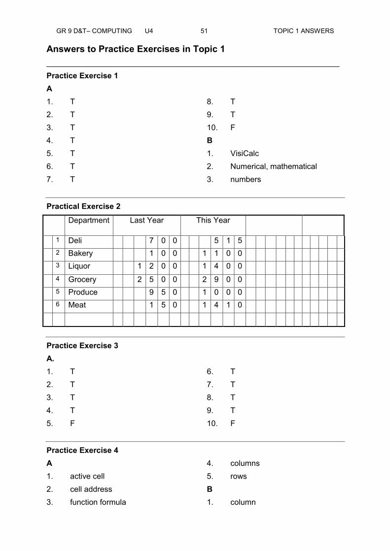
Answers to Practice Exercises in Topic 1 ___________________________________________________________________ Practice Exercise 1 A 1. T 2. T 3. T 4. T 5. T 6. T 7. T
8. T 9. T 10. F B 1. VisiCalc 2. Numerical, mathematical 3. numbers
Practical Exercise 2
Department Last Year This Year
1 Deli 7 0 0 5 1 5
2 Bakery 1 0 0 1 1 0 0
3 Liquor 1 2 0 0 1 4 0 0
4 Grocery 2 5 0 0 2 9 0 0
5 Produce 9 5 0 1 0 0 0
6 Meat 1 5 0 1 4 1 0
Practice Exercise 3 A. 1. T 2. T 3. T 4. T 5. F
6. T 7. T 8. T 9. T 10. F
Practice Exercise 4 A 1. active cell 2. cell address 3. function formula
4. columns 5. rows B 1. column

GR 9 D&T– COMPUTING U4 52 TOPIC 1 ANSWERS
2. ribbons 3. cell address
4. rows 5. up or down
Practice Exercise 5 A 1. T 2. T 3. T 4. T 5. F
B 1. f 2. d 3. g 4. a 5. b 6. e 7. c
Practice Exercise 6 A
1. New - used to create a new Workbook.
2. Open- used to open an existing file from a flash drive or hard drive of your computer.
3. Close- used to close a Spreadsheet.
4. Save As- used when to save a new file for the first time or save an existing file with a different name. 5. Save- used to save a file that has had changes made to it. If you close the workbook without saving then any changes made will be lost. B 1. Choose File from the menu bar.
2. Click Save as with your mouse.
3. Choose My Documents on top of the Filename box.
4. Create a new folder by clicking the right mouse button and choose New.
5. Choose Folder to create a new folder.
6. Type Excel Practise as your folder name.
End of Topic 1.
Now Do Exercise 1 in Assignment Book 1 Then Go to Topic 2.

GR 9 D&T– COMPUTING U4 53 TOPIC TITLE
TOPIC 2
CREATING A SAMPLE WORKSHEET
Lesson 7 : Setting Up Rows and Columns in a Spreadsheet
Lesson 8 : Entering Data and Formula in a Spreadsheet
Lesson 9 : Adding and Deleting Rows and/or Columns in a Spreadsheet
Lesson 10: Editing Data in a Spreadsheet Lesson 11: Setting Cell Attributes in a
Spreadsheet Lesson 12: Sorting Data in a Spreadsheet

GR 9 D&T– COMPUTING U4 54 TOPIC INTRODUCTION
TOPIC 2: CREATING A SAMPLE WORKSHEET ___________________________________________________________________ In this topic you will learn about setting up rows and columns and entering data and formula. This topic is designed for you to understand how to enter data in a cell and to set up columns and rows. The aim is for you to gain an understanding of the basics of entering and sorting data in a Spreadsheet.
Data entry is one of the things for which Excel is widely used. Making a data entry form that prohibits inaccurate data entry from users is straightforward in Excel.
Spreadsheet (such as Microsoft Excel) can help you track budgets, inventories or misuse of funds on your personal computer. If you need to store formulas and enter in different numbers on a regular basis, you could use a pencil and a calculator. But the problem of entering in the wrong data is that to recalculate every formula over again.
Because Microsoft Office comes with Excel, you may as well get your money’s worth and use a Spreadsheet to help you calculate numbers instead. To use a Spreadsheet, just type in numbers, create formulas and then add labels to help you understand what specific numbers represent. After you do that, you may want to format your numbers and labels to make them look more presentable.
In this topic you will study the following:
Lesson 7 focuses on setting up rows and columns. You will learn how to define and identify rows and columns and set them in a Spreadsheet.
Lesson 8 presents the definition of cell, data and formula. You will learn how to distinguish among cell, data and formula especially how to type the data in a cell and explain the meaning of formula in Spreadsheet.
Lesson 9 discusses on adding and deleting rows and columns. You will learn the steps in adding and deleting rows and columns in a Spreadsheet. You will further learn the benefits of adding and deleting rows and columns.
Lesson 10 explains editing data. You will learn the importance of editing data in a Spreadsheet.
Lesson 11 concentrates on setting up cell attributes. You will learn the definition and importance of setting up cell attributes. You will also learn how to identify the different cell attributes and apply them appropriately.
Lesson 12 discusses on sorting data. You will learn the meaning and importance of sorting data.
By the end of Topic 2, you should be able to correctly use design and create a Spreadsheet for a particular purpose and create your own simple work.

GR 9 D&T– COMPUTING U4 55 TOPIC 2 LESSON 7
Lesson 7: Setting Up Rows and Columns in a Spreadsheet ___________________________________________________________________
___________________________________________________________________ Microsoft Excel Versions Before we can begin to discuss how to set up rows and columns, let us first distinguish the different versions of Microsoft Excel. These will enable you to understand their differences and thereby learn the required skills.
1. Microsoft Excel version 2003 The standard amount of columns has been 256. They are labelled by letters of the alphabet. After Z you get AA, AB, AC etc. until you get to AZ. Then BA, BB, BC and so on. The 256th column is IV. All together there are 65,536 numbered rows that make 16,777,216 cells.
Note: There should be no space when using comma in writing numbers.
2. Microsoft Excel version 2007
In Excel 2007 the maximum number of rows per worksheet increased to 1,048,576 and the number of columns increased to 16,384 which is column XFD. That makes 17,179,869,184 cells.
Excel 2010 has the same number of rows and columns.
3. Microsoft Excel 2010 In Excel 2010 the maximum number of rows per worksheet is up to 1,048,576 and the number of columns is up to 16,384 which is column XFD. That makes 17,179,869,184 cells.
From the above you can see that Microsoft Excel versions 2007 and 2010 have the same number of rows and columns.
Your Aims:
define rows and columns
define cell address
select a cell or cells
set up rows and columns
Welcome to Lesson 7 of Unit 4. In Lesson 6, you learned how to save a workbook in different locations and exit an Excel workbook.
In this lesson you will define rows, columns, cell and be able to categorise the different versions of Microsoft Excel.
GR 9 D&T– COMPUTING U4 56 TOPIC 2 LESSON 7
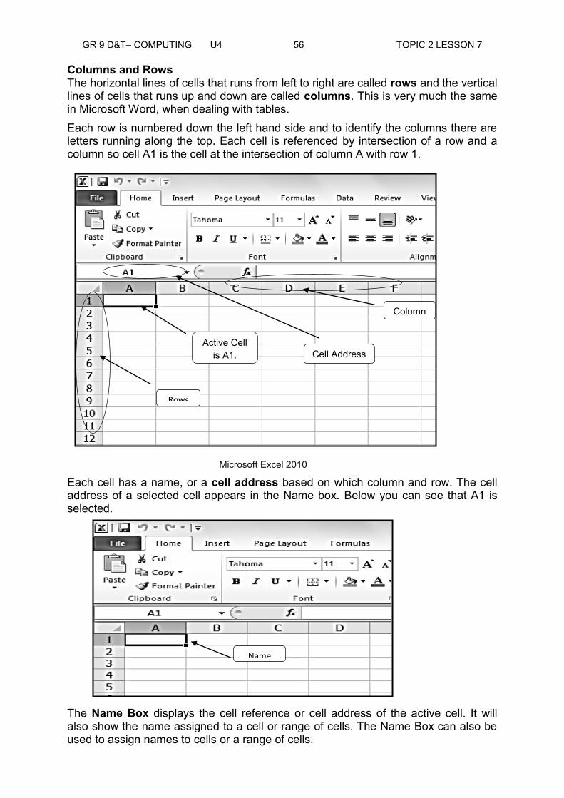
Columns and Rows The horizontal lines of cells that runs from left to right are called rows and the vertical lines of cells that runs up and down are called columns. This is very much the same in Microsoft Word, when dealing with tables. Each row is numbered down the left hand side and to identify the columns there are letters running along the top. Each cell is referenced by intersection of a row and a column so cell A1 is the cell at the intersection of column A with row 1.
Each cell has a name, or a cell address based on which column and row. The cell address of a selected cell appears in the Name box. Below you can see that A1 is selected.
The Name Box displays the cell reference or cell address of the active cell. It will also show the name assigned to a cell or range of cells. The Name Box can also be used to assign names to cells or a range of cells.
Rows
Cell Address
Columns
Active Cell is A1.
Microsoft Excel 2010
Name
Box

GR 9 D&T– COMPUTING U4 57 TOPIC 2 LESSON 7
Selecting a Cell The following are steps on how to select a cell.
1. Click on a cell to select it. When a cell is selected you will notice that the borders of the cell appear bold and the column heading and the row heading of the cell are highlighted. 2. Release your mouse. The cell will stay selected until you click on another cell in the worksheet You can also navigate through your worksheet and select a cell by using the arrow keys on your keyboard. Selecting Multiple Cells The following are steps on how to select multiple cells.
1. Click and drag your mouse until all of the adjoining cells you want are highlighted. Release your mouse. The cells will stay selected until you click on another cell in the worksheet.
Selecting Multiple Cells
Modifying Column Width 1. Position your mouse over the column line in the column heading. You will notice that your mouse will change from white cross to double arrow. Start dragging your mouse to your left if you want to reduce. Drag your mouse to your right if you want to widen your column. Look at the picture below which further illustrates this.

GR 9 D&T– COMPUTING U4 58 TOPIC 2 LESSON 7
Adjusting Row height 1. Position your mouse on the row line in the row heading. You will notice that your mouse will change from white cross to double arrow. You can start dragging your mouse from up or down to reduce or to widen the row height. Look at the picture below which further illustrates this.
Activity 1. Provide the information in the table for the three versions of Microsoft Excel.
Version MS – Excel 2003 MS – Excel 2007 MS – Excel 2010
Rows
Columns
Total Number of Cells
Activity 2: Practice moving the mouse into different cells and adjusting column width and row height.
Sample Keyboard
The Double Arrow

GR 9 D&T– COMPUTING U4 59 TOPIC 2 LESSON 7
1. Using your mouse, start to click from column A in row 1, and proceed along clicking each cell until you reach the cell in column F row 1.
As you will notice, the cell address from the Name box changed from A1 to F1 and the active cell moved to cell address F1. If your screen looks like the one in the picture above then you did the right thing.
2. Next, from cell F1 press the down arrow key seven times then three times to your left using the left arrow key.
So, from F1 we moved the cell address to C8.
3. Next, is to practice adjusting the column width by placing your mouse double arrow to the end of column C and move your mouse to your right towards column D.
Cell address Active cell

GR 9 D&T– COMPUTING U4 60 TOPIC 2 LESSON 7
4. To practice adjusting the row height by placing your double arrow to row heading 3 and move your mouse downward to widen the row height.
Thank you for completing this activity. Make sure you did the right thing by looking at the pictures. ___________________________________________________________________
Activity 3: Practice selecting multiple cells.
1. Open a new Excel workbook.
2. Click on A1, hold down your mouse and drag your mouse pointer to cell D5.
You will notice that cells B1 to D5 are selected. If your screen looks like the one in the picture above then you did the right thing. Thank you for completing this activity. Make sure you did the right thing by looking back at the picture on page 69. ___________________________________________________________________
Summary You have come to the end of Lesson 7. In this lesson, you have learnt the definitions of rows, columns and cell. You have also learnt about selecting cells or multiple cells in Excel.
NOW DO PRACTICE EXERCISE 7 ON THE NEXT PAGE.

GR 9 D&T– COMPUTING U4 61 TOPIC 2 LESSON 7
Practice Exercise: 7
Part A: Circle the letter of the correct answer.
1. What Microsoft Excel version has 256 columns?
A. MS Excel version 2003 B. MS Excel version 2007
C. MS Excel version 2010 D. None of the above
2. What is the total number of cells in MS Excel version 2003?
A. 16,777,612 cells B. 16,777,216 cells
C. 16,776,216 cells D. 16,767,216 cells
3. What is the maximum number of rows per worksheet in MS Excel 2007?
A. 1,048,576 rows B. 1,048,675 rows
C. 1,084,576 rows D. 1,048,555 rows
4. Which MS Excel version has 16,384 columns?
A. MS Excel version 2003
B. MS Excel version 2007
C. MS Excel version 2010
D. MS Excel versions 2007 and 2010
5. For MS Excel version 2003, what is the 256th column?
A. IX B. IV
C. XX D. ZZ
6. For MS Excel version 2007, what is the 16,384th column?
A. XYZ B. XGD
C. XFD D. XDF
7. Choose the correct order form in MS Excel columns.
A. AA, AB, AD, AE B. AA, AC, AE, AG
C. AA, AB, AC, AD D. AA, AB, AC, AE
8. The total number of cells for MS Excel version 2010 is ___________.
A. 17,179,869,184 B. 17,000,000,184
GR 9 D&T– COMPUTING U4 62 TOPIC 2 LESSON 7
C. 17,179,869,148 D. None of the above
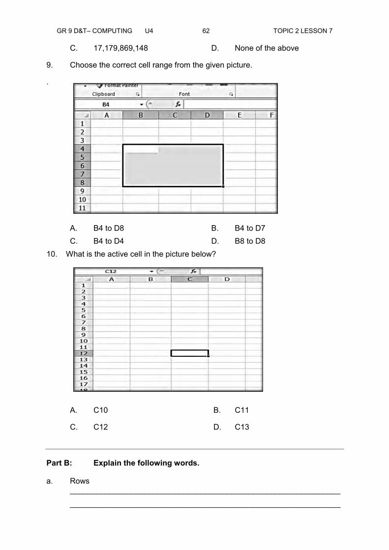
9. Choose the correct cell range from the given picture.
.
A. B4 to D8 B. B4 to D7 C. B4 to D4 D. B8 to D8 10. What is the active cell in the picture below?
A. C10 B. C11
C. C12 D. C13
Part B: Explain the following words. a. Rows ______________________________________________________________
______________________________________________________________

GR 9 D&T– COMPUTING U4 63 TOPIC 2 LESSON 7
b. Columns ______________________________________________________________
______________________________________________________________
c. Cell Address ______________________________________________________________
______________________________________________________________
d. Active Cell ______________________________________________________________
______________________________________________________________
e. Name Box ______________________________________________________________
______________________________________________________________
CHECK YOUR WORK. ANSWERS ARE AT THE END OF TOPIC 2.
GR 9 D&T– COMPUTING U4 64 TOPIC 2 LESSON 8
Lesson 8: Entering Data and Formula in a Spreadsheet ___________________________________________________________________
Welcome to lesson 8 of Unit 2, In Lesson 7, you learnt about the definitions of rows, columns and cell. You have also learnt about selecting cells or multiple cells in Excel. In this lesson you will define cell, data, and formula and enter data and formula in a cell.
____________________________________________________________ The Cell Content Each cell can contain its own text, formatting, comments, formulas and functions.
Text - Cells can contain letters, numbers, and dates
Formatting Attributes – Cells can contain formatting attributes that change the way letters, numbers, and dates are displayed. For example, dates can be formatted as MM/DD/YYYY or Month/D/YYYY
Comments – Cells can contain comments from multiple reviewers.
Formula and Functions – Cells can contain formulas and functions that calculate cell values. For example, SUM (cell 1, cell 2…) is a formula that can add the values in multiple cells.
Now let us go back and try to type the given data from Lesson 2 Unit 4 of our lesson.
The given data:
Department Last Year This Year
Deli 700 515 Bakery 1000 1100 Liquor 1200 1400 Grocery 2500 2900 Produce 950 1000 Meat 1500 1410 1. Let us begin by typing the data in cell address A1 which is Department. Enter content into the selected cell using your keyboard (A1). The content appears in the cell and in the formula bar. You can also enter or edit cell content from the formula bar.
Your Aims: type data
define formula
enter formula in a cell

GR 9 D&T– COMPUTING U4 65 TOPIC 2 LESSON 8
2. Since Department is longer than the cell, you need to adjust cell A1 to fit in the cell content.
3. Continue to type Last Year in cell B1 and This Year in cell C1.
This is how it will look like after typing the three data into the first row.
Formula
Bar
Cell

GR 9 D&T– COMPUTING U4 66 TOPIC 2 LESSON 8
4. Continue to type the content starting from row 3 onwards as follows.
This is how it will look like after typing the content. Modifying the Row Height Modifying the row height enables you to have the cell contents fit in the cell. Follow
the steps below on how to modify the row height.
1. Position the cursor over the bottom of the row line so that the white cross becomes a double arrow .
2. Click hold down and drag the row downward to increase the row height or upward decrease the row height. 3. Release the mouse. The height of each selected row will change in your worksheet.

GR 9 D&T– COMPUTING U4 67 TOPIC 2 LESSON 8
Creating Simple Formulas Excel can be used to calculate numerical information. In this section you will learn how to create simple formulas in Excel to add, subtract, multiply and divide values in a workbook.
Also, you will learn about many ways you can use cell references to make working with formulas easier and more efficient.
Definition of Formula A formula is a mathematical expression that performs a calculation. Like a calculator, Excel can execute formulas that add, subtract, multiply and divide.
One of the most useful features of Excel is its ability to calculate using the cell address to represent the value in a cell. This is call cell reference.
In order to make full use of the capabilities of Excel, it is important to know how to create simple formulas using cell references.
Creating Simple Formulas Now that you know the definition of formula, you can now learn the steps on how to create formula using Excel.
Excel uses standard operators for equations, such as a plus sign for addition (+), a minus sign for subtraction (-), an asterisk for multiplication (*), a forward slash for division (/) and a carat (^) for exponents.
The key thing to remember when writing formulas for Excel is that all formulas must begin with an equal sign (=). This is because the cell contains or is equal to the formula and its value. Study the table below.
Mathematical Operations Symbols Sample Equations
Addition + =5+5
Subtraction - =5-5
Multiplication * =5*5
Division / =5/5
Exponents ^ =5^5
The formula you need to type should be a combination of numbers and letters representing the columns and rows that we will use either to add, subtract, multiply, divide or depending to our needs.

GR 9 D&T– COMPUTING U4 68 TOPIC 2 LESSON 8
Creating a Simple Formula in Excel The following steps will enable you to create simple formula using Excel. 1. Select the cell where the answer will appear.
Example in D3.
2. Type the equal sign (=). 3. Type in the formula you want to calculate. Suppose you will compute for the total for Deli on cell D3, type either on the Formula Bar or within cell D3 (=700+515).
Whatever we will type in our active cell will also appear in our Formula Bar. We can do editing of our text or formula using the Formula Bar.
Formula Bar
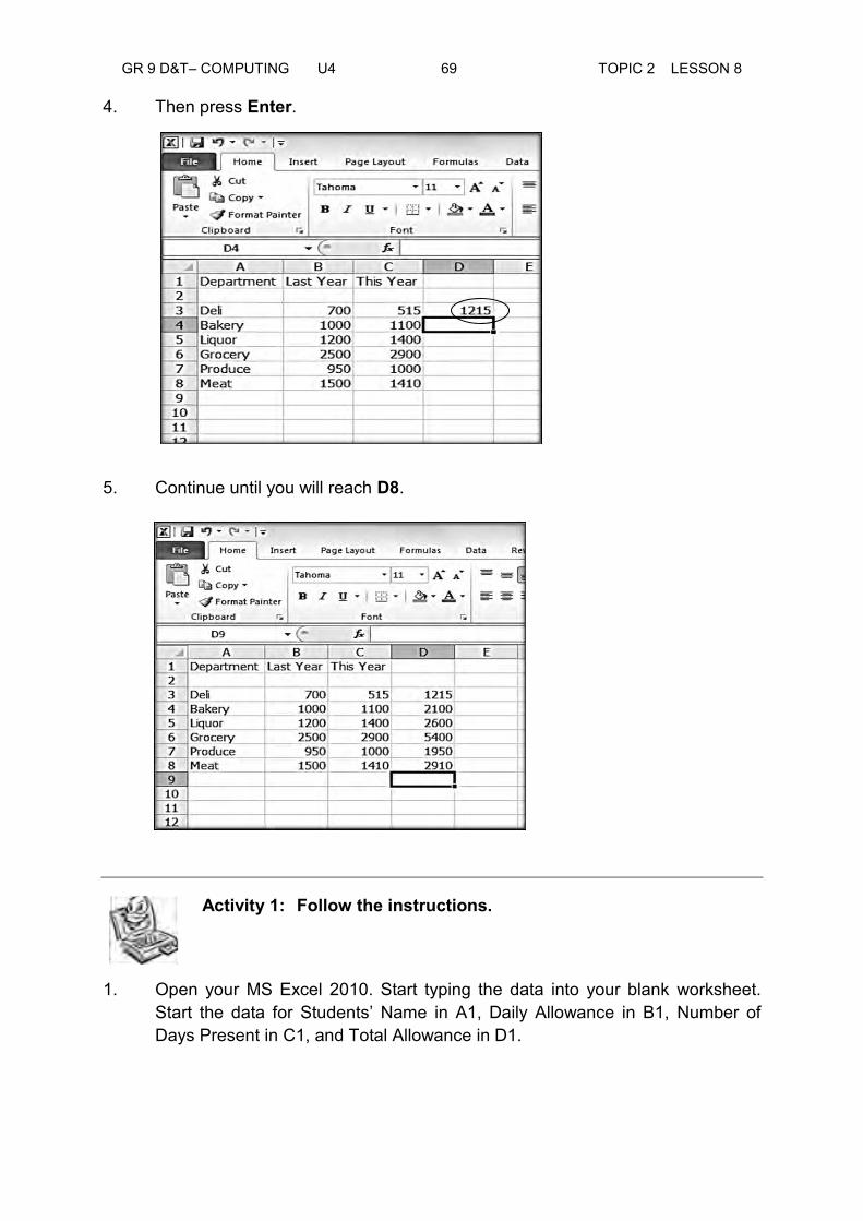
GR 9 D&T– COMPUTING U4 69 TOPIC 2 LESSON 8
4. Then press Enter.
5. Continue until you will reach D8.
Activity 1: Follow the instructions.
1. Open your MS Excel 2010. Start typing the data into your blank worksheet. Start the data for Students’ Name in A1, Daily Allowance in B1, Number of Days Present in C1, and Total Allowance in D1.
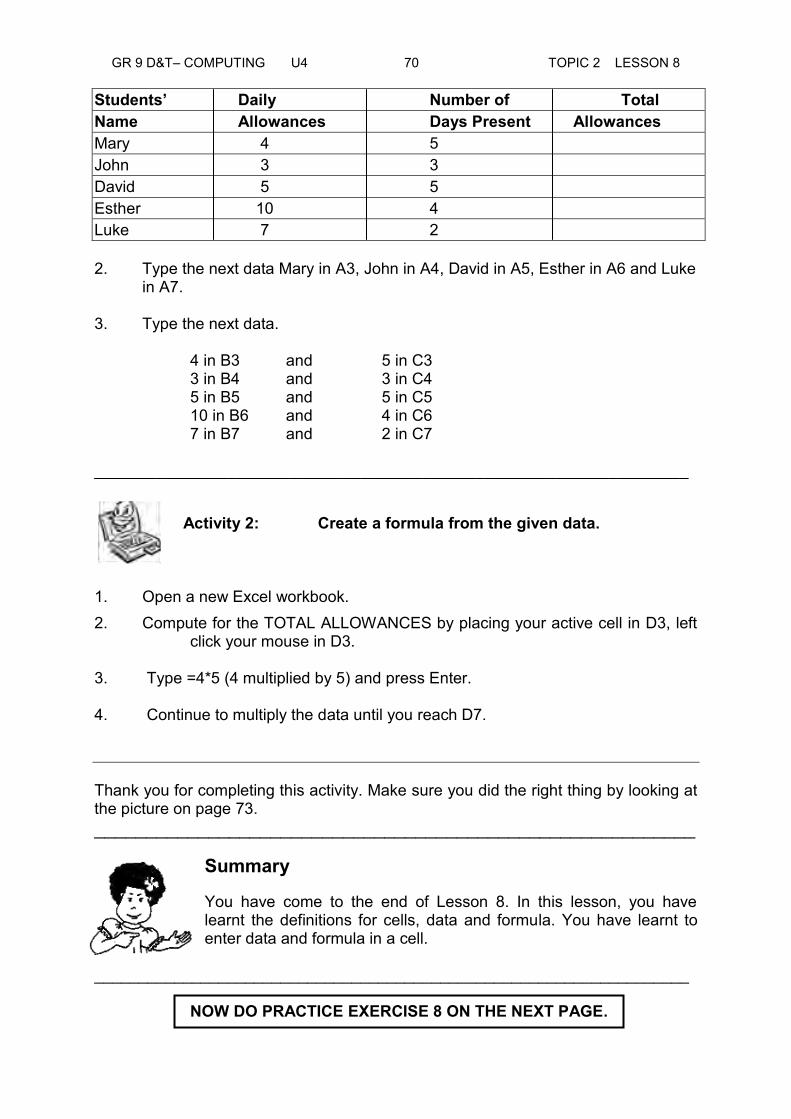
GR 9 D&T– COMPUTING U4 70 TOPIC 2 LESSON 8
Students’ Daily Number of Total Name Allowances Days Present Allowances Mary 4 5 John 3 3 David 5 5 Esther 10 4 Luke 7 2 2. Type the next data Mary in A3, John in A4, David in A5, Esther in A6 and Luke in A7. 3. Type the next data. 4 in B3 and 5 in C3 3 in B4 and 3 in C4 5 in B5 and 5 in C5 10 in B6 and 4 in C6 7 in B7 and 2 in C7 ___________________________________________________________________
Activity 2: Create a formula from the given data.
1. Open a new Excel workbook. 2. Compute for the TOTAL ALLOWANCES by placing your active cell in D3, left
click your mouse in D3. 3. Type =4*5 (4 multiplied by 5) and press Enter. 4. Continue to multiply the data until you reach D7. Thank you for completing this activity. Make sure you did the right thing by looking at the picture on page 73. __________________________________________________________
Summary
You have come to the end of Lesson 8. In this lesson, you have learnt the definitions for cells, data and formula. You have learnt to enter data and formula in a cell.
___________________________________________________________________ NOW DO PRACTICE EXERCISE 8 ON THE NEXT PAGE.

GR 9 D&T– COMPUTING U4 71 TOPIC 2 LESSON 8
Practice Exercise: 8
A Match the symbols in Column A with their meaning in Column B. write the correct answer on the blank space beside each symbol.
A B 1. + _______ a. Carat 2. – _______ b. Forward Dash 3. * _______ c. Asterisk 4. / _______ d. Minus 5. ^ _______ e. Plus 6. or _______ f. White cross 7. _______ g. Double arrow
B Define the following.
a. Formula Bar ______________________________________________________________
______________________________________________________________
______________________________________________________________
b. Cell Reference ______________________________________________________________
______________________________________________________________
______________________________________________________________
c. Text ______________________________________________________________
______________________________________________________________
______________________________________________________________
d. Formula ______________________________________________________________
______________________________________________________________
______________________________________________________________
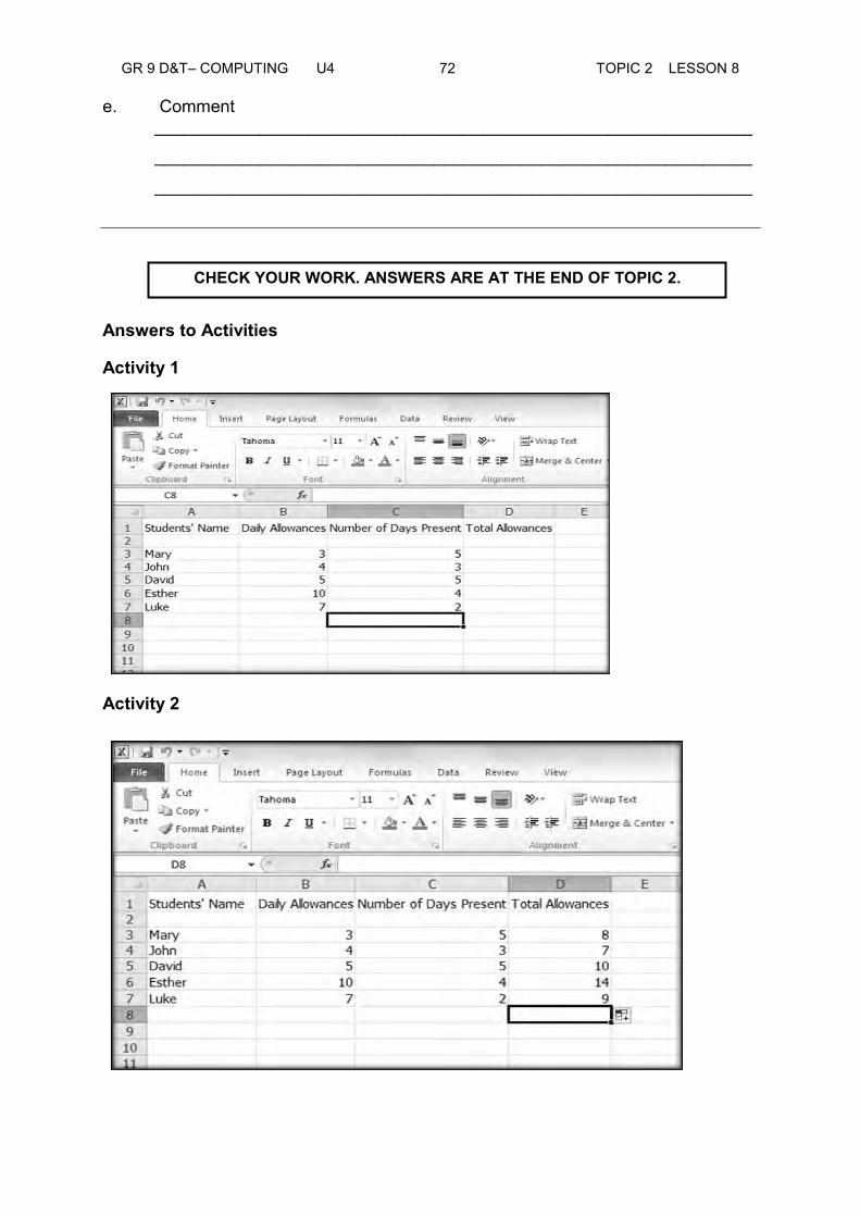
GR 9 D&T– COMPUTING U4 72 TOPIC 2 LESSON 8
e. Comment ______________________________________________________________
______________________________________________________________
______________________________________________________________
Answers to Activities
Activity 1
Activity 2
CHECK YOUR WORK. ANSWERS ARE AT THE END OF TOPIC 2.

GR 9 D&T– COMPUTING U4 73 TOPIC 2 LESSON 9
Lesson 9: Adding and Deleting Rows and/or Columns ___________________________________________________________________
Welcome to Lesson 9 of Unit 2. In Lesson 8, you learnt about the definitions of cells, data and formula. You have also learnt to enter data and formula in a cell. In this lesson you will insert rows and columns, delete rows and columns and identify the importance of adding and deleting rows and/or columns.
Your Aims:
The Importance of Adding and Deleting Rows and/or Columns The following are important in adding and deleting rows and columns.
Adding or deleting a row is important to reflect the change in a worksheet.
Adding or deleting columns can help keep your worksheet organised.
There are times when you need to alter the appearance of a worksheet by inserting or deleting rows or columns of data.
Inserting Rows 1. Select the row below where you want the new row to appear.
Selecting the Row
insert rows and columns delete rows and columns identify the importance of adding and deleting
rows and columns

GR 9 D&T– COMPUTING U4 74 TOPIC 2 LESSON 9
2. Click the Insert command on the Home tab. 1 2
Selecting the Insert Cells Command. After clicking your left mouse button. 3
Choosing Insert Cells with your mouse.
3. Click Enter, and the new row appears in your worksheet.
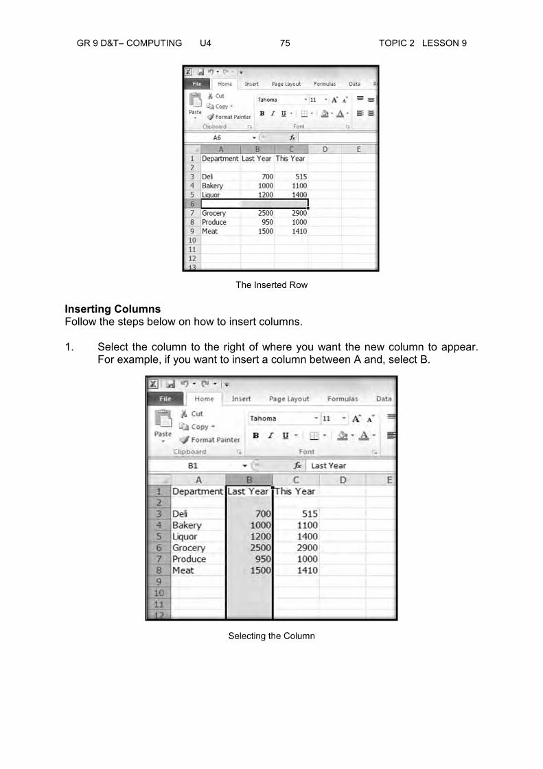
GR 9 D&T– COMPUTING U4 75 TOPIC 2 LESSON 9
The Inserted Row
Inserting Columns Follow the steps below on how to insert columns. 1. Select the column to the right of where you want the new column to appear. For example, if you want to insert a column between A and, select B.
Selecting the Column

GR 9 D&T– COMPUTING U4 76 TOPIC 2 LESSON 9
2. Select the Insert command on the Home tab. 1 2
Selecting the Insert Cells Command. After clicking your left mouse button. 3
By choosing Insert Sheet Columns with your mouse.
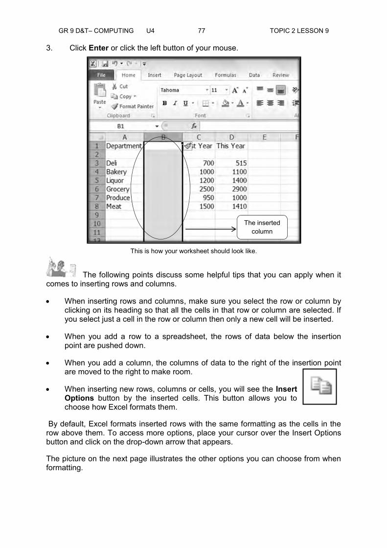
GR 9 D&T– COMPUTING U4 77 TOPIC 2 LESSON 9
3. Click Enter or click the left button of your mouse.
This is how your worksheet should look like.
The following points discuss some helpful tips that you can apply when it comes to inserting rows and columns.
When inserting rows and columns, make sure you select the row or column by clicking on its heading so that all the cells in that row or column are selected. If you select just a cell in the row or column then only a new cell will be inserted.
When you add a row to a spreadsheet, the rows of data below the insertion point are pushed down.
When you add a column, the columns of data to the right of the insertion point are moved to the right to make room.
When inserting new rows, columns or cells, you will see the Insert Options button by the inserted cells. This button allows you to choose how Excel formats them.
By default, Excel formats inserted rows with the same formatting as the cells in the row above them. To access more options, place your cursor over the Insert Options button and click on the drop-down arrow that appears.
The picture on the next page illustrates the other options you can choose from when formatting.
The inserted column

GR 9 D&T– COMPUTING U4 78 TOPIC 2 LESSON 9
Deleting Rows Follow the steps on how to delete rows. 1. Select the rows you want to delete.
Selecting the row

GR 9 D&T– COMPUTING U4 79 TOPIC 2 LESSON 9
2. Click the Delete command on the Home tab. 1 2
Selecting the Delete command. After clicking your left mouse button. 3
By choosing Delete Sheet Rows with your mouse.
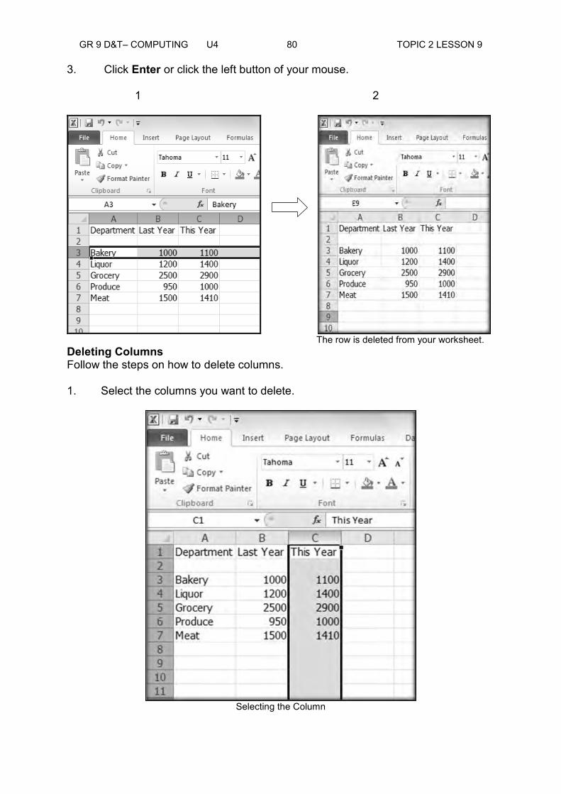
GR 9 D&T– COMPUTING U4 80 TOPIC 2 LESSON 9
3. Click Enter or click the left button of your mouse. 1 2
The row is deleted from your worksheet.
Deleting Columns Follow the steps on how to delete columns. 1. Select the columns you want to delete.
Selecting the Column

GR 9 D&T– COMPUTING U4 81 TOPIC 2 LESSON 9
2. Click the Delete command on the Home tab. 1 2
Selecting the Delete command. After clicking your left mouse button. 3. Click Enter or click the left button of your mouse.
After the column was deleted from your worksheet.

GR 9 D&T– COMPUTING U4 82 TOPIC 2 LESSON 9
Activity 1: Follow the instructions to complete this activity.
Inserting Rows 1. Enter the following data into your MS Excel: The first data which is ITEMS in cell reference A1. Proceed to the next data No. of Items in B1, Price in C1, and Total in D1. Followed with the other contents from the ITEMS, No. of Items, and Price T-shirts in A2 25 in B2 22 in C2 Short Pants in A3 30 in B3 26 in C3 Socks in A4 25 in B4 12 in C4 Caps in A5 33 in B5 15 in C5 2. Insert rows for every line by clicking your mouse in your row heading 2.
3. Select the Insert command on the Home tab.
4. Select the Insert Sheet Rows, and click your left mouse button.
5. Continue to insert rows which are in row 4, and follow steps 3 and 4.
6. Continue to insert rows which are in row 6, and follow steps 3 and 4.
7. Continue to insert rows which are in row 8, and follow steps 3 and 4.
Inserting Columns 1. Insert columns before TOTAL by clicking your left button mouse in your Column Heading D.
2. Select the Insert command on the Home tab. Click the Insert Sheet Columns.
___________________________________________________________________
Thank you for completing this activity. Go to the end of the lesson to check your answers.
Activity 2: Follow the instructions to complete this activity.
1. Let us go back to our Activity 1 by deleting the spaces in a worksheet.

GR 9 D&T– COMPUTING U4 83 TOPIC 2 LESSON 9
2. Place your mouse in Row Heading 2. Click the Delete command on the Home tab. 3. Click Delete Sheet Rows by the Left button of your mouse.
4. Continue placing your mouse to the next row to be deleted until you will reach the last row. Deleting Columns 1. Select the columns you want to delete, the Column Heading D.

GR 9 D&T– COMPUTING U4 84 TOPIC 2 LESSON 9
2. Click the Delete command on the Home tab. Click the Delete Sheet Columns.
Thank you for completing this activity. Go to the end of the lesson to check your answers.
Summary
You have come to the end of Lesson 9. In this lesson, you have learnt how to insert rows and columns and delete rows and
columns. You have also learnt about and the importance of adding and deleting rows and columns in Excel.
___________________________________________________________________
NOW DO PRACTICE EXERCISE 9 ON THE NEXT PAGE.
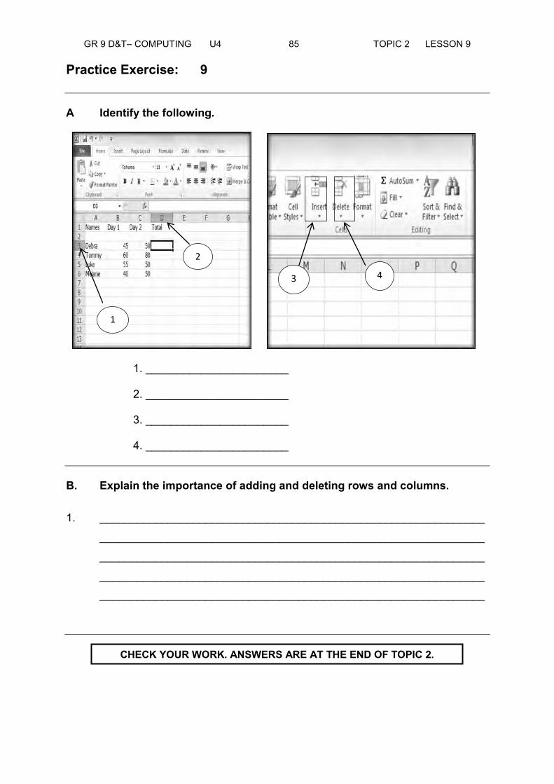
GR 9 D&T– COMPUTING U4 85 TOPIC 2 LESSON 9
Practice Exercise: 9 A Identify the following.
1. _______________________ 2. _______________________ 3. _______________________ 4. _______________________ B. Explain the importance of adding and deleting rows and columns.
1. ______________________________________________________________
______________________________________________________________
______________________________________________________________
______________________________________________________________
______________________________________________________________
1
2
3 4
CHECK YOUR WORK. ANSWERS ARE AT THE END OF TOPIC 2.

GR 9 D&T– COMPUTING U4 86 TOPIC 2 LESSON 9
Answers to Activity:
Activity 1 1.
After typing the data
4.
After clicking the Insert Sheet Rows After inserting the rows
Inserting Columns
1.
2.
7.
The Column Heading Cell D

GR 9 D&T– COMPUTING U4 87 TOPIC 2 LESSON 9
2.
The Inserted Columns
Activity 2
3.
Deleting Rows The Deleted Rows
Deleting Columns
2.
4.
After deleting the column

GR 9 D&T– COMPUTING U4 88 TOPIC 2 LESSON 10
Lesson 10: Editing Data
___________________________________________________________________
Welcome to lesson 10 of Unit 2. In Lesson 9, you learnt about how to insert and delete rows and columns. You have also learnt about the importance of adding and deleting rows and columns in Excel. In this lesson you will identify the importance of editing data. You will also learn how to edit and change data in a Spreadsheet.
Your Aims:
Editing and Changing Data For correcting a mistake or updating data, you can edit the data in your worksheet. Meaning of Editing Editing is changing the data; there is another way of changing the data by changing its appearance. You can change the font and fill colour of the data. Steps to remember:
1. Double click on the cell containing the data you want to edit. A flashing insertion point appears in the cell.
edit data
change data

GR 9 D&T– COMPUTING U4 89 TOPIC 2 LESSON 10
2. Press the arrow keys on the keyboard to move the insertion point to where you want to remove or add characters.
3. To remove the character to the left of the flashing insertion point, press the Backspace key.
To remove the character to the right of the of the flashing insertion point, press the Delete key.
4. To add data where the insertion point flashes on your screen, type the data.
5. When you finish making changes to the data, press the Enter key.
Deleting Data You can remove unnecessary data from the cells of your worksheet. You can delete data from a single cell or from several cells at once.
1. Select the cell or cells containing the data you want to delete.
2. Press the Delete key.
The data disappears from the cells you had selected.
Changing the Font Many of the commands you will use can be found in the Font, Alignment and the Number groups on the ribbon. Font commands let you change the style, size and colour of text. You can also use them to add borders and fill colours to cells. Number commands let you change selected cells that display numbers and dates.
Let us use our data from the filename ITEM. Open your filename ITEM.
1. Select the cells you want to edit by placing your mouse onto the first row and click the left button of the mouse.

GR 9 D&T– COMPUTING U4 90 TOPIC 2 LESSON 10
2. Click the drop-down arrow next to the font command on the Home tab. The font drop-down menu appears.
Changing the Font
3. Move your mouse over the various fonts. A live preview of the font will appear in the worksheet. 4. Select the font you want to use. Select Algerian as your new font for Row 1 of your worksheet.
Font drop down menu
Algerian Font

GR 9 D&T– COMPUTING U4 91 TOPIC 2 LESSON 10
5. Highlight Column A2 to A5 to change for the new font.
6. Click the Font drop-down menu again.
7. Select the font you want to use.
Select Bradley Hand ITC as your new font for Column 1 of your worksheet.

GR 9 D&T– COMPUTING U4 92 TOPIC 2 LESSON 10
After selecting the new font.
8. Highlight the numbers from B2 to C5 to change the font and Bold the data.
9. Click the Font drop-down menu again.
10. Select Times New Roman as your new font.
Bradley Hand ITC

GR 9 D&T– COMPUTING U4 93 TOPIC 2 LESSON 10
11. Next, click Bold to highlight the numbers.
After selecting the new font click Bold.
12. Compute for the Total.
13. Place the active cell to D2 and from the Formula Bar type, =B2+C2 and press Enter.
14. Do the same to D3, D4 and D5 to get the Total.
The result after typing the formula.

GR 9 D&T– COMPUTING U4 94 TOPIC 2 LESSON 10
15. Since our Total is not bolded, let us highlight the Total with yellow by clicking the Fill Colour.
16. Highlight D2 to D5.
17. Click Fill Colour and choose Yellow for our Total.
Yellow
While choosing your colour, a live preview will appear in your worksheet.

GR 9 D&T– COMPUTING U4 95 TOPIC 2 LESSON 10
After clicking the Fill Colour
18. Save our work by naming this as ITEM2.
19. From our File Menu, click Save As.
20. As you may have noticed, Book1 was highlighted as a suggested filename for your work. Press Backspace from the keyboard to change it with your filename ITEM2.

GR 9 D&T– COMPUTING U4 96 TOPIC 2 LESSON 10
21. Press Save.
Activity 1: Follow the instructions to complete the activity.
1. Open a new Excel workbook and type the given data.
List of Groceries Quantity Price Total
Tomato 2 kg. 8.50/kg Banana 1 kg. 7/kg Cereals 1 Box 6.70/box Orange Juice 1 Litre 10.50/litre Bread 2 Loaves 3.50/loaf Sugar 3 kg. 5.10/kg
2. Edit column 1 (A1 to D1) by changing our font to Broadway. Highlight column 1 and click the Font drop down menu to Broadway.
3. Adjust the title List of Groceries by positioning your mouse in between columns A and B and use to adjust your columns to the right. Do the same to Quantity. 4. Change the font A3 to A8 by highlighting A3 to A8 and click again the Font Drop down menu and select Tahoma.

GR 9 D&T– COMPUTING U4 97 TOPIC 2 LESSON 10
5. Bold the List of Groceries.
6. Change the font for B3 to C8. Highlight B3 to C8 and click the Font Drop down menu to select the font. This time let us use Forte as our font style for this data.
7. Compute the Total using the Formula Bar.
8. Place the active cell in D3 and type from the Formula Bar =2*3.5, we cannot make the formula addressing the cell because the given data had a combination of numbers and letters.
9. Continue multiplying the quantity and price until you will reach D8.
10. It is time for us to highlight the total and use the Text Highlight Colour. Click the Text Highlight Drop Down menu and select Orange for the Total.
11. Save our work under the filename ITEM3. Click the File Menu and Select Save As. Type ITEM3.
Thank you for completing this activity. Go to the end of this lesson to check your answers.
Summary You have come to the end of Lesson 10. In this lesson, you have learnt how to identify the importance of editing data and change data in a Spreadsheet.
___________________________________________________________________
NOW DO PRACTICE EXERCISE 10 ON THE NEXT PAGE.

GR 9 D&T– COMPUTING U4 98 TOPIC 2 LESSON 10
Practice Exercise: 10
A Identify the following.
1. ______________________________________ 2. ______________________________________ 3. ______________________________________ 4. ______________________________________ 5. ______________________________________
B Name the steps on how to change the font of a data in Excel.
1. ______________________________________________________________
______________________________________________________________
1
2
3 4
5
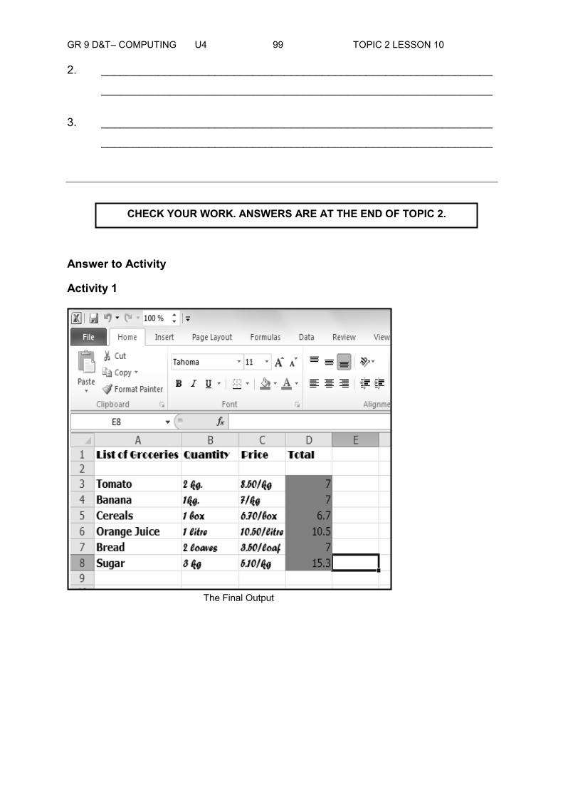
GR 9 D&T– COMPUTING U4 99 TOPIC 2 LESSON 10
2. ______________________________________________________________
______________________________________________________________
3. ______________________________________________________________
______________________________________________________________
Answer to Activity
Activity 1
The Final Output
CHECK YOUR WORK. ANSWERS ARE AT THE END OF TOPIC 2.

GR 9 D&T– COMPUTING U4 100 TOPIC 2 LESSON 11
Lesson 11: Setting up Cells Attributes
___________________________________________________________________
Welcome to Lesson 11 of Unit 2. In Lesson 10, you learnt the importance of editing data. You have also learnt to compare data in cells and compare the changes with the original. In this lesson you will define cell attributes, identify the different cell attributes and apply the appropriate cell attributes.
Your Aims:
Cell Attributes Spreadsheet does not include a variety of text formatting options contained in word processing software. However, there still exists a need for variety for the easy comparison of different types of data. For example, the headings on a Spreadsheet should be distinct from the actual figures. Cell attributes allows a user to define the appearance of Spreadsheet. We can apply text attributes and cell borders in Excel. We can also change the text attribute of a heading which is one way to add contrast. Thus, it is now easy to differentiate between the types of data. In addition, cell borders can be used to visually separate data.
The cell reference is the particular cell (or a range) for which the attribute value need to be returned. If a range is used, the attribute value for the top-left cell is returned.
The text attribute refers to how a particular font is presented. For instance, we might use the bold attribute to emphasize our text, or italics might be used to indicate a term being defined. In Excel it refers to as the font styles. The most common attributes can be applied with a few of the tools available on the Formatting toolbar. And there are three text attribute tools provided Bold, Italic and Underline.
The attribute type that you are trying to find can be colour, column/row position, width, format or a number of other attributes. Only one attribute can be specified in a single formula.
Editing Cell Contents Using long labels might cut off some part of the data. When you enter a label wider than the cell it occupies, the excess text appears to spill into the next cell to the right-unless there is data in the adjacent cell. If the adjacent cell contains data, the label will be cut off and see only the portion of the label that fits in the cell’s current width.
define cell attributes
identify different cell attributes apply appropriate cell attributes
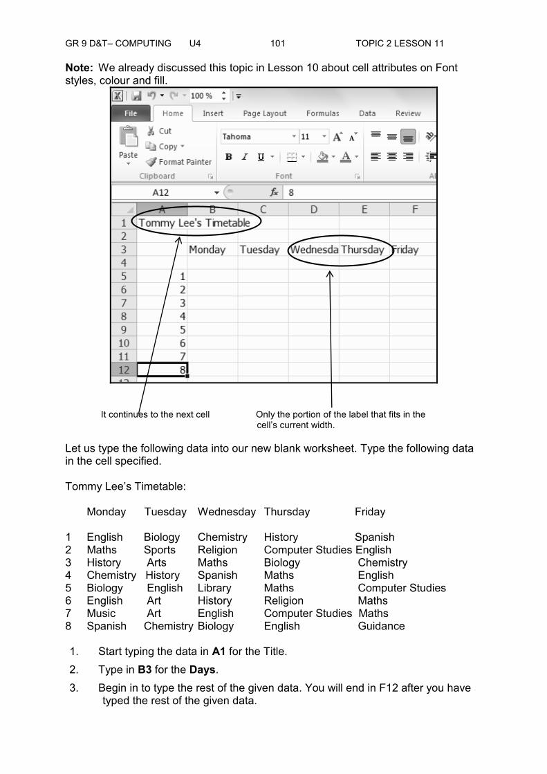
GR 9 D&T– COMPUTING U4 101 TOPIC 2 LESSON 11
Note: We already discussed this topic in Lesson 10 about cell attributes on Font styles, colour and fill.
It continues to the next cell Only the portion of the label that fits in the cell’s current width. Let us type the following data into our new blank worksheet. Type the following data in the cell specified. Tommy Lee’s Timetable: Monday Tuesday Wednesday Thursday Friday 1 English Biology Chemistry History Spanish 2 Maths Sports Religion Computer Studies English 3 History Arts Maths Biology Chemistry 4 Chemistry History Spanish Maths English 5 Biology English Library Maths Computer Studies 6 English Art History Religion Maths 7 Music Art English Computer Studies Maths 8 Spanish Chemistry Biology English Guidance 1. Start typing the data in A1 for the Title. 2. Type in B3 for the Days. 3. Begin in to type the rest of the given data. You will end in F12 after you have
typed the rest of the given data.
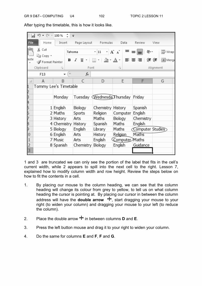
GR 9 D&T– COMPUTING U4 102 TOPIC 2 LESSON 11
After typing the timetable, this is how it looks like.
1 and 3 are truncated we can only see the portion of the label that fits in the cell’s current width, while 2 appears to spill into the next cell to the right. Lesson 7, explained how to modify column width and row height. Review the steps below on how to fit the contents in a cell.
1. By placing our mouse to the column heading, we can see that the column heading will change its colour from grey to yellow, to tell us on what column heading the cursor is pointing at. By placing our cursor in between the column address will have the double arrow , start dragging your mouse to your right (to widen your column) and dragging your mouse to your left (to reduce the column).
2. Place the double arrow in between columns D and E.
3. Press the left button mouse and drag it to your right to widen your column.
4. Do the same for columns E and F, F and G.

GR 9 D&T– COMPUTING U4 103 TOPIC 2 LESSON 11
After adjusting the columns
1
2
3

GR 9 D&T– COMPUTING U4 104 TOPIC 2 LESSON 11
5. Save your worksheet with the filename Timetable1.
To Set Column Width with a Specific Measurement Follow the steps on how to set the column width with a specific measurement. 1. Select the columns you want to modify.
2. Click the Format command on the Home tab. The format drop-down menu appears.
3. Select Column Width.

GR 9 D&T– COMPUTING U4 105 TOPIC 2 LESSON 11
4. The Column Width dialog box appears. Enter a specific measurement.
5. Change the column width (10.25) to 15.
6. Click OK. The width of each selected column will be changed in your worksheet. Select AutoFit Column Width from the format drop-down menu and Excel will automatically adjust each selected column so that all the text will fit.
7. Adjust columns C, D, E and F. Follow step 1 again and adjust the columns.
After adjusting the columns.

GR 9 D&T– COMPUTING U4 106 TOPIC 2 LESSON 11
To Set Row Height with a Specific Measurement: There are two ways of setting row height with specific measurements. The first way consists of 5 steps and the second one is selecting Auto Fit Row Height. Follow the steps on how to set the row with the specific measurement.
1. Select the rows you want to modify.
2. Click the Format command on the Home tab. The format drop-down menu appears.
3. Select Row Height.
4. The Row Height dialog box appears. Enter a specific measurement. Change it to 30.
5. Click OK. The selected row heights will be changed in your Spreadsheet.
Do the same for the rest of the rows by changing B3 to F3 to 25.
Change A5 to F12 to 20.
After adjusting all the rows
1 2
3

GR 9 D&T– COMPUTING U4 107 TOPIC 2 LESSON 11
Select AutoFit Row Height from the format drop-down menu and Excel will automatically adjust each selected row so that all the text will fit.
Activity 1. Fill-in the blanks to answer the items below.
1. Changing the text attribute of a heading is one way to add contrast. Thus, you can easily differentiate the types of data. In addition, ______________ can be used to visually separate data.
2. The _________________ is the particular cell (or a range) for which the attribute value need to be returned. If a range is used, the ________________ value for the top-left cell is returned.
3. The _________________ refers to how a particular font is presented. For instance, we might use the bold attribute to emphasize our ______________, or ____________ might be used to indicate a term being defined. In Excel it is referred to as the _________________.
4. The most common attributes can be applied with a few of the tools available on the Formatting toolbar. And there are three text attribute tools provided __________________, _____________ and ________________;
GR 9 D&T– COMPUTING U4 108 TOPIC 2 LESSON 11
5. The ________________ attribute that you are trying to find. It can be ____________, ______________ position, width, format or a number of other attributes. Only one attribute can be specified in a single formula.
___________________________________________________________________
Thank you for completing this activity. Now, you may go to the end of this lesson to check your answers. Make sure you do the necessary corrections before moving on to the next part of this lesson.
Summary
You have come to the end of Lesson 11. In this lesson you defined cell attributes, identified different cell attributes and applied appropriate cell attributes.
NOW DO PRACTICE EXERCISE 11 ON THE NEXT PAGE.
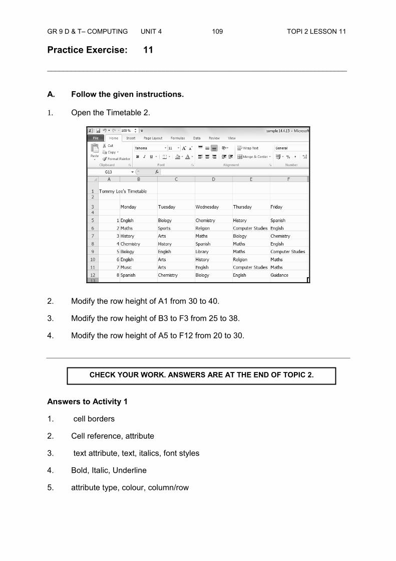
GR 9 D & T– COMPUTING UNIT 4 109 TOPI 2 LESSON 11
Practice Exercise: 11
___________________________________________________________________________
A. Follow the given instructions. 1. Open the Timetable 2.
2. Modify the row height of A1 from 30 to 40.
3. Modify the row height of B3 to F3 from 25 to 38.
4. Modify the row height of A5 to F12 from 20 to 30.
Answers to Activity 1
1. cell borders
2. Cell reference, attribute
3. text attribute, text, italics, font styles
4. Bold, Italic, Underline
5. attribute type, colour, column/row
CHECK YOUR WORK. ANSWERS ARE AT THE END OF TOPIC 2.

GR 9 D&T– COMPUTING U4 110 TOPIC 2 LESSON 12
Lesson 12: Sorting Data
__________________________________________________________________________
Welcome to Lesson 12 of Unit 4. In Lesson 11, you defined cell attributes, identified applied different attributes.
In this lesson you will learn the definition of sorting, identify how it is done and apply it properly using the given rubrics or guidelines.
Your Aims:
Sorting Sorting is reordering of data. It is a common task in Spreadsheet. The most common type of sorting is alphabetical ordering, which you can do in ascending or descending order. To Sort in Alphabetical Order Follow the steps in sorting in alphabetical order.
1. Select a cell in the column you want to sort (In this example, we choose a cell in column B).
identify and define what sorting is
apply skills in sorting data

GR 9 D&T– COMPUTING U4 111 TOPIC 2 LESSON 12
2. Click the Sort & Filter command in the Editing group on the Home tab.
3. Select Sort A to Z. Now the information in the Category column is organised
in alphabetical order.
4. After selecting Sort A to Z this dialogue box will appear. Click Sort.

GR 9 D&T– COMPUTING U4 112 TOPIC 2 LESSON 12
After clicking Sort A to Z.
5. You can Sort in reverse alphabetical order by choosing Sort Z to A in the list.
After clicking Sort Z to A.
7. Save your work with the filename Sort1.

GR 9 D&T– COMPUTING U4 113 TOPIC 2 LESSON 12
To Sort from Smallest to Largest Follow the steps on how to sort from smallest to largest.
1. Select a cell in the column you want to sort (a column with numbers).
Let us consider our sample worksheet Sort1.
2. Click the Sort & Filter command in the Editing group on the Home tab.
3. Select From Smallest to Largest. Now the information is organised from the
smallest to largest amount.
4. Click Sort.

GR 9 D&T– COMPUTING U4 114 TOPIC 2 LESSON 12
After clicking From Smallest to Largest.
5. You can sort in reverse numerical order by choosing From Largest to Smallest in the list.
6. Click Sort.

GR 9 D&T– COMPUTING U4 115 TOPIC 2 LESSON 12
7. Save your work with the filename Sort2.
Activity 1 Answer the given questions.
1. Discuss the steps on how to sort text from A to Z using sort
command. ______________________________________________________________
______________________________________________________________
______________________________________________________________
______________________________________________________________
______________________________________________________________
______________________________________________________________
2. Discuss the steps on how to sort numbers from Largest to Smallest.
______________________________________________________________
______________________________________________________________
______________________________________________________________
______________________________________________________________
______________________________________________________________
______________________________________________________________
Thank you for completing this activity. Now, you may go to the end of this lesson to check your answers. Make sure you do the necessary corrections before moving on to the next part of this lesson.
Summary
You have come to the end of Lesson 12. In this lesson you learnt the definition of sorting and how to sort data from A to Z and Z to A and from smallest to largest and from largest to smallest.
NOW DO PRACTICE EXERCISE 12 ON THE NEXT PAGE.

GR 9 D&T– COMPUTING U4 116 TOPIC 2 LESSON 12
Practice Exercise: 12
______________________________________________________________
A. Sort the given data in Excel.
No. Employee’s Name Annual Salary (Kina) 1. Rodillas, Raymart 45250 2. Pua, John Jeremy 55630 3. Pei, Elmerson David 88230 4. Randol, Robert 71019 5. Amari, Albert Mark 35050 6. Bonbon, Neil Johnny 56450
1. Sort the Employee’s Name from A to Z. Sort the numbers from largest to smallest.
2. Sort the Annual Salary from Largest to Smallest.
Answers to Activity 1 Sort from A to Z a. Select a cell in the column you want to sort.
b. Click the Sort & Filter command in the Editing group on the Home tab.
c. Select Sort A to Z. Now the information in the Category column is organised in alphabetical order.
d. Click Sort.
e. Save your work.
2. Sort from Largest to Smallest
a. Select a cell in the column you want to sort (a column with numbers).
b. Click the Sort & Filter command in the Editing group on the Home tab.
c. Select From Largest to Smallest. Now the information is organised from the largest to smallest amount.
d. Click Sort.
e. Save your work.
CHECK YOUR WORK. ANSWERS ARE AT THE END OF TOPIC 2.
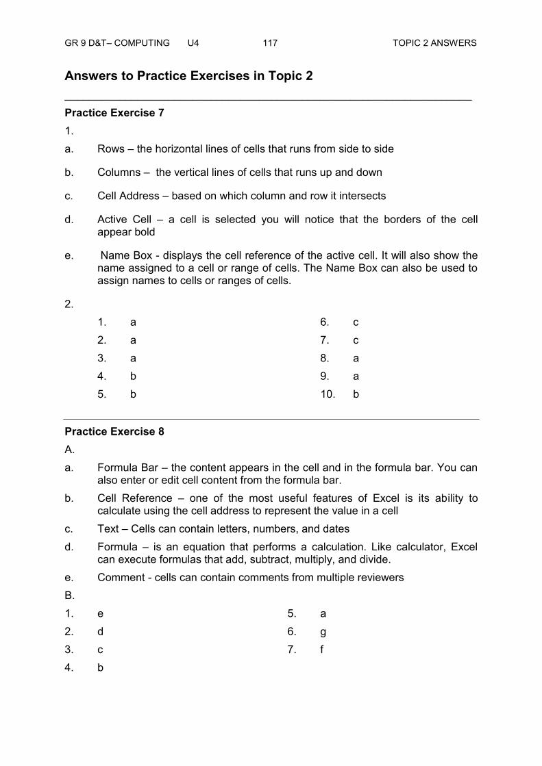
GR 9 D&T– COMPUTING U4 117 TOPIC 2 ANSWERS
Answers to Practice Exercises in Topic 2 ___________________________________________________________________ Practice Exercise 7 1. a. Rows – the horizontal lines of cells that runs from side to side
b. Columns – the vertical lines of cells that runs up and down
c. Cell Address – based on which column and row it intersects
d. Active Cell – a cell is selected you will notice that the borders of the cell appear bold
e. Name Box - displays the cell reference of the active cell. It will also show the name assigned to a cell or range of cells. The Name Box can also be used to assign names to cells or ranges of cells.
2. 1. a 2. a 3. a 4. b 5. b
6. c 7. c 8. a 9. a 10. b
Practice Exercise 8 A. a. Formula Bar – the content appears in the cell and in the formula bar. You can
also enter or edit cell content from the formula bar. b. Cell Reference – one of the most useful features of Excel is its ability to
calculate using the cell address to represent the value in a cell c. Text – Cells can contain letters, numbers, and dates d. Formula – is an equation that performs a calculation. Like calculator, Excel
can execute formulas that add, subtract, multiply, and divide. e. Comment - cells can contain comments from multiple reviewers B. 1. e 2. d 3. c 4. b
5. a 6. g 7. f

GR 9 D&T– COMPUTING U4 118 TOPIC 2 ANSWERS
Practice Exercise 9 A. a. row
b. column c. Insert command d. Delete command
B. Any of the following answers will do. a. Adding or deleting a row is important to reflect the change in a
worksheet. b. Adding or deleting columns can help keep your worksheet organised. c. There are times when you need to alter the appearance of a worksheet
by inserting additional rows or columns of data.
Practice Exercise 10
A. 1. Drop down arrow menu for font style 2. Font Style 3. Fill Colours 4. Drop down arrow for Fill colour 5. Formula Bar B.
1. Select the cells you want to edit by placing your cursor onto the first row and click the left button of the mouse.
2. Click the drop down arrow next to the font command on the Home tab. The font drop down menu appears.
3. A little preview of the font will appear, select the font you want to use.
Practice Exercise 11

GR 9 D&T– COMPUTING U4 119 TOPIC 2 ANSWERS
Practice Exercise 12
A.
B.
End of Topic 2
Now Do Exercise 2 in Assignment Book 2 Then Go to Topic 3.

GR 9 D&T– COMPUTING U4 120 TOPIC TITLE
TOPIC 3
MAKING SIMPLE CALCULATIONS
Lesson 13 : Adding Numbers in Various Cells Lesson 14 : Subtracting Numbers in Various
Cells Lesson 15 : Multiplying Numbers in Various
Cells Lesson 16 : Dividing Two Numbers Lesson 17 : Using Auto Sum Lesson 18 : Copying Data or Formula

GR 9 D&T– COMPUTING U4 121 TOPIC INTRODUCTION
TOPIC 3: MAKING SIMPLE CALCULATIONS
___________________________________________________________________
In this topic you will learn about adding, subtracting, multiplying and dividing numbers in various cells.
Excel includes powerful mathematical formulas to display trends using specified equation from large data sets. These formulas can become extremely complex and by default an Excel formula is not easy to read.
The reader of a spreadsheet generally trusts the author to complete spreadsheet calculations accurately. An unethical Excel practice is to allow calculation errors to go unfixed if their displayed results are more favourable, or to deliberately hide such errors in calculations deep within formulas to make them difficult to find.
Ethical practices require fixing all mathematical errors as they are discovered and naming cell ranges in Excel so that formulas are as easy to read as possible by all people using the spreadsheet.
Lesson 13 focuses on adding numbers in various cells. You will learn how to add and calculate the sum of given numbers in various cells.
Lesson 14 discusses on subtracting numbers in various cells. You will learn how to subtract and calculate the difference of given numbers in various cells.
Lesson 15 elaborates on multiplying numbers in various cells. You will learn how to multiply and identify the benefits gained in multiplying numbers using MS Excel.
Lesson 16 gives explanations about dividing two numbers from the formula in Excel. You will learn how to divide numbers in various cells and identify the benefits gained in dividing numbers using MS Excel.
Lesson 17 explains the use of Auto sum. You will learn what is Auto Sum and its purpose, enumerate the steps for using Auto Sum, use Auto Sum to add numbers in various cells and identify the benefits gained in using Auto Sum in a Spreadsheet.
Lesson 18 emphasises on copying data or formula. You will learn how to copy data or formula, perform Copying Data or Formula from various cells and identify the benefits gained in using Copying Data or Formula operation in a Spreadsheet.
By the end of Topic 3, you should be able to compute and use various formulas for the given data.
GR 9 D&T– COMPUTING U4 122 TOPIC 3 LESSON 13
Lesson 13: Adding Numbers in Various Cells
_________________________________________________________________________
Welcome to lesson 13 of Unit 4. In Lesson 12, you identified the steps of sorting data and sorted data using the given rubrics or guidelines.
In this lesson you will be able to describe the steps of adding numbers to calculate the sum in numbers in various cells.
Your Aims:
identify the process of adding numbers in various cells
add numbers in various cells
Calculations in Excel
A formula is an equation that performs a calculation. Like a calculator, Excel can execute formulas that add, subtract, multiply and divide.
One of the most useful features of Excel is its ability to calculate using a cell address to represent the value in a cell. This is called using a cell reference.
In order to maximize the capabilities of Excel, it is important to understand how to create simple formulas and use cell reference.
Excel uses standard operators for equations, such as a plus sign for addition (+), a minus sign for subtraction (-), an asterisk for multiplication (*), a forward slash for division (/), and a carat (^) for exponents.
The key thing to remember when writing formulas for Excel is that all formulas must begin with an equal sign (=). This is because the cell contains, or is equal to, the formula and its value.
Addition of Numbers in various cells Follow the instructions below on how to add numbers in various cells.
1. Enter the information in a Spreadsheet. Be sure that the information is entered in the same cells as the given sample next page, or the formulas will not work. Make sure to adjust the column width to fit the text in each cell.
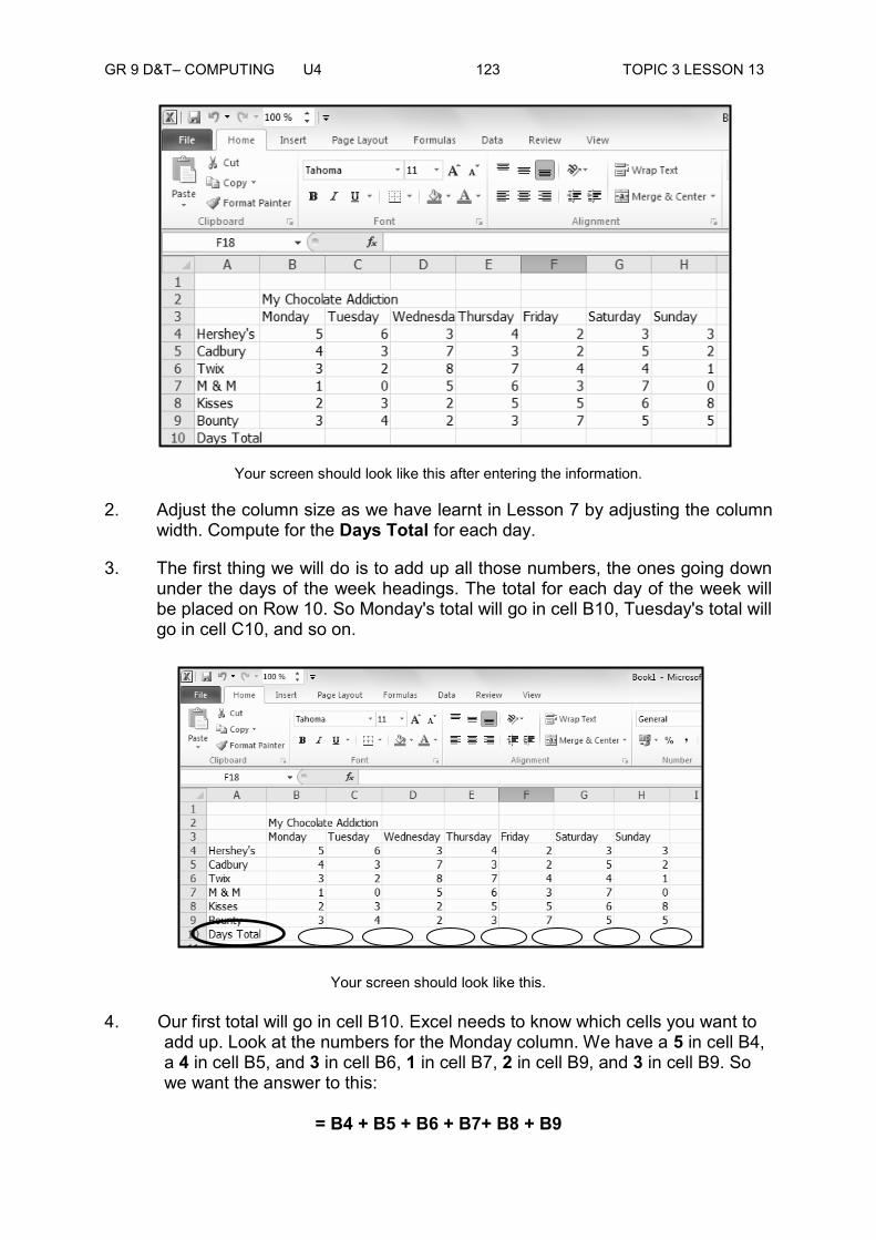
GR 9 D&T– COMPUTING U4 123 TOPIC 3 LESSON 13
Your screen should look like this after entering the information.
2. Adjust the column size as we have learnt in Lesson 7 by adjusting the column width. Compute for the Days Total for each day.
3. The first thing we will do is to add up all those numbers, the ones going down under the days of the week headings. The total for each day of the week will be placed on Row 10. So Monday's total will go in cell B10, Tuesday's total will go in cell C10, and so on.
Your screen should look like this.
4. Our first total will go in cell B10. Excel needs to know which cells you want to add up. Look at the numbers for the Monday column. We have a 5 in cell B4, a 4 in cell B5, and 3 in cell B6, 1 in cell B7, 2 in cell B9, and 3 in cell B9. So we want the answer to this:
= B4 + B5 + B6 + B7+ B8 + B9
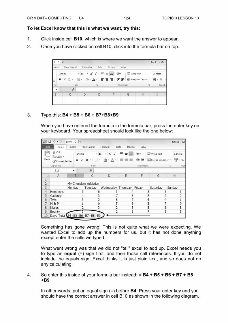
GR 9 D&T– COMPUTING U4 124 TOPIC 3 LESSON 13
To let Excel know that this is what we want, try this:
1. Click inside cell B10, which is where we want the answer to appear. 2. Once you have clicked on cell B10, click into the formula bar on top.
3. Type this: B4 + B5 + B6 + B7+B8+B9
When you have entered the formula in the formula bar, press the enter key on your keyboard. Your spreadsheet should look like the one below:
Something has gone wrong! This is not quite what we were expecting. We wanted Excel to add up the numbers for us, but it has not done anything except enter the cells we typed.
What went wrong was that we did not "tell" excel to add up. Excel needs you to type an equal (=) sign first, and then those cell references. If you do not include the equals sign, Excel thinks it is just plain text, and so does not do any calculating.
4. So enter this inside of your formula bar instead: = B4 + B5 + B6 + B7 + B8 +B9
In other words, put an equal sign (=) before B4. Press your enter key and you should have the correct answer in cell B10 as shown in the following diagram.

GR 9 D&T– COMPUTING U4 125 TOPIC 3 LESSON 13
5. Move your mouse to the next cell which is C10, do the same steps for step 4 but change column B to C, and so on until you will reach column H.
Your screen should look like this after clicking Enter for cell B10.
6. Save your worksheet with the filename Addition1.
7. Let us also add one column to the right to get the TOTAL for the whole week for every brand of chocolates.

GR 9 D&T– COMPUTING U4 126 TOPIC 3 LESSON 13
8. Place our active cell to I4 and type =B4 + C4 + D4 + E4 + F4 + G4 + H4 + I4
9. Click Enter.
Your screen should look like this after clicking Enter.
10. Continue to add the TOTAL for cells I5 to I9 by following step 8.
11. Save your worksheet with the filename Addition2.

GR 9 D&T– COMPUTING U4 127 TOPIC 3 LESSON 13
Activity 1. Refer to the following information then answer question that follow.
1. A cell in a Spreadsheet has a cell reference B2. What is the column and what is the row in the reference?
______________________________________________________________
______________________________________________________________
______________________________________________________________
2. Write down what is contained in the following cells of the sample Spreadsheet.
a. A4 ________________
b. A6 ________________
c. B7 ________________
d. C6 ________________
e. A9 ________________
3. Write down the cell reference for:
a. Saturday _________________
b. Pop Corn _________________
c. 45 _________________
d. 15 _________________
e. 10 _________________
4. Write the formula for the Total for Saturday. ________________

GR 9 D&T– COMPUTING U4 128 TOPIC 3 LESSON 13
5. Write the formula for the Total for Monday. _________________
6. Solve for the Total by typing the data into your Excel and apply the formula you wrote for 4 and 5. ________________
Thank you for completing this activity. Now, you may go to the end of this lesson to check your answer. Make sure you do the necessary corrections before moving on to the next part of this lesson.
Summary
You have come to the end of Lesson 13. In this lesson you learnt how to add numbers in various cells using the formula bar.
NOW DO PRACTICE EXERCISE 13 ON THE NEXT PAGE.

GR 9 D&T– COMPUTING U4 129 TOPIC 3 LESSON 13
Practice Exercise: 13
___________________________________________________________________
A. Follow the given instructions below to complete the exercise.
1. Open an Excel workbook and type the given data.
B2 Grade 10 Class A, Term2 Marks
A4 Name
B4 Science B5 20
C4 Maths C5 20
D4 English D5 20
E4 IT E5 20
F4 Buss. Studies F5 20
G4 TOTAL G5 100
A6 1 B6 Abby, Bobby
A7 2 B7 Bobo, John
A8 3 B8 Cad, David
A9 4 B9 Dove, Mark
A10 5 B10 Fumi, Michaelyn
A11 6 B11 Farrah, Debra
A12 7 B12 Gomez, Natalie
A13 8 B13 Heinz, Lucy
A14 9 B14 Jazz, Mary
A15 10 B15 Komah, Beth
2. Compute for the TOTAL by adding all the subjects.
3. Save your work with the filename Students’ Marks.
CHECK YOUR WORK. ANSWERS ARE AT THE END OF TOPIC 3.

GR 9 D&T– COMPUTING U4 130 TOPIC 3 LESSON 13
Answers to Activity 1
1.
2. a. Tickets
b. Drinks
c. 3
d. 5
e. Total
3. a. B3
b. A5
c. B4
d. B5
e. C5
4. =B4+B5+B6+B7
5. =C4+C5+C6+C7
6.
Column
Row
GR 9 D&T– COMPUTING U4 131 TOPIC 3 LESSON 14
Lesson 14: Subtracting Numbers in Various Cells _________________________________________________________________________
Welcome to lesson 14 of Unit 4. In Lesson 13 you learnt how to add numbers in various cell references using the formula bar.
In this lesson you will be able to subtract numbers in various cell references.
Your Aims:
identify the process of subtracting numbers in various cells
subtract numbers in various cells _________________________________________________________________________
Writing the Formula The key thing to remember when writing formulas for Excel is that all formulas must begin with an equal sign (=). This is because the cell contains, or is equal to, the formula and its value. Remember to always place your cursor in the cell where you want to place your answer.
Remember this rule as we take the next step in using Excel in calculating.
Subtraction of Numbers in Various Cells Follow the instructions on how to subtract number in various cells.
First let us type the given data into our Excel.
A Headmaster of a school asked one of the teachers to count the number of the students who are present today at school, and deduct it from the number of students who are absent.
1. Type this data into your Excel.
Cell References Data A2 Attendance for Today
C4 No. of Students
D4 Absent for Today
E4 No. Of Present
A5 Grade 9 Class A
A6 Grade 9 Class B
A7 Grade 9 Class C
A8 Grade 10 Class A
A9 Grade 10 Class B

GR 9 D&T– COMPUTING U4 132 TOPIC 3 LESSON 14
A10 Grade 10 Class C
C5 50
C6 51
C7 52
C8 50
C9 50
C10 45
D5 7
D6 8
D7 5
D8 4
D9 3
D10 6
2. Modify the title to font type Algerian.
3. Adjust the column width to fit into your data into the cell.

GR 9 D&T– COMPUTING U4 133 TOPIC 3 LESSON 14
4. Compute for the number of present students by deducting the number of students to the absent for today. From the formula function, type, = C5 – D5
5. Click Enter.
6. Do the same to E6, E7, E8, E9 and E10.
After subtracting the No. of Students to Absent for Today.
7. Save your work with the filename Subtraction1.
Activity 1. Using the given data, solve for the following.
The Manager of Hideaway Hotel asked for a report for the number of confirmed guests for the next week’s big holiday. This is in order to know the number of rooms available for that week.
1. Type the data into your Excel.
A1 Hideaway Port Moresby
B3 No. of Rooms
C3 Confirmed Guests
D3 No. of Available Rooms
A4 Twin Share Room
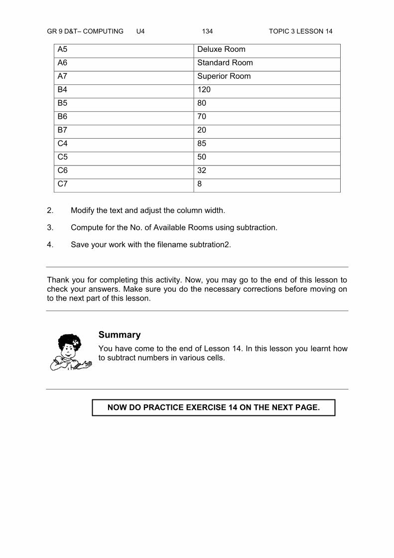
GR 9 D&T– COMPUTING U4 134 TOPIC 3 LESSON 14
A5 Deluxe Room
A6 Standard Room
A7 Superior Room
B4 120
B5 80
B6 70
B7 20
C4 85
C5 50
C6 32
C7 8
2. Modify the text and adjust the column width.
3. Compute for the No. of Available Rooms using subtraction.
4. Save your work with the filename subtration2.
Thank you for completing this activity. Now, you may go to the end of this lesson to check your answers. Make sure you do the necessary corrections before moving on to the next part of this lesson.
Summary You have come to the end of Lesson 14. In this lesson you learnt how to subtract numbers in various cells.
NOW DO PRACTICE EXERCISE 14 ON THE NEXT PAGE.

GR 9 D&T– COMPUTING U4 135 TOPIC 3 LESSON 14
Practice Exercise: 14
___________________________________________________________________
A. Make a table using Excel to compute for the following given data:
1. Cell reference C2, Title: Subtraction
B3, Data1
C3, Data2
D3, Answer
2. Cell references A5 to A11 type a to g
B5, 185 C5, 89
B6 10788 C6, 9854
B7 1256 C7, 995
B8, 89562 C8, 75210
B9, 45221 C9, 36000
B10, 2354 C10, 1896
B11, 895 C11, 788
Answers to Activity
CHECK YOUR WORK. ANSWERS ARE AT THE END OF TOPIC 3.

GR 9 D&T– COMPUTING U4 136 TOPIC 3 LESSON 15
Lesson 15: Multiplying Numbers in Various Cells
_________________________________________________________________________
Welcome to lesson 15 of Unit 4. In Lesson 14 you learnt how to subtract numbers in various cell references.
In this lesson you will be able to multiply numbers in various cell references.
Your Aims: identify the process of multiplying numbers in
various cells
multiply numbers in various cells
_________________________________________________________________________
Multiplication of Numbers in Various Cells Formulas are the heart of Excel. With huge list of built-in formula and functions, Excel stands out from other datasheet handling applications. Formulas are used for calculating and analysing data based on values in designated cells. It supports trigonometric, statistical and other functions. You can also create a new rule, or constraint to apply over your datasheet. This post covers writing formulas and applying conditional formatting on a basic level.
You learnt from Lesson 13 that the symbol for our multiplication is an asterisk ( * ). You can find it on top of number keys on your keyboard by pressing the Shift key and at the same time the number 8 key.
As we already learnt the addition and the subtraction we will also follow the same approach for multiplication. Remember to always put your cursor in the cell where you want to put your answer.
1. Type the following given data into your Excel.
Mrs Jones asked her housemaid to buy some groceries for dinner tonight. Here is the list of groceries for Mrs Jones.
Grocery Lists
ITEMS Pieces Price per Item (Kina) Total
1. Whole Chicken 3 12
2. Loaves of Bread 4 6
3. Soft drinks 4 10
4. Ice Cream 2 20
5. Butter 2 8 6. Thick Cream 3 6

GR 9 D&T– COMPUTING U4 137 TOPIC 3 LESSON 15
2. Modify the text, and adjust the column width.
3. Compute for the Total using multiplication process.
This is how your screen should look like after multiplying columns C and D.
4. Save your work with the filename Multiplication1.
Activity 1. Refer to the information below to complete this activity.
The BIG BOSS Company computed for the number of hours for the following student trainees in order for them to issue their training allowances complying for the number of hours for their on-the-job training.
The BIG BOSS Company
Name of Trainees Rate per hour Number of Hours Total
1. Den More 3 20
2. Alvin Mamaki 2 18
3. Mary Bob 3 25

GR 9 D&T– COMPUTING U4 138 TOPIC 3 LESSON 15
4. Elizabeth Dondon 2 30
5. Elisa Ninimo 2 22
1. Open an Excel workbook and type the given data.
2. Modify the text and adjust the column width.
3. Solve for the Total by multiplying the number of hours by the rate per hour per trainee.
= C3 * D3
4. Press Enter.
5. Do the same computations for C4 to C7 by multiplying to column D.
6. Save your work with the filename Multiply1.
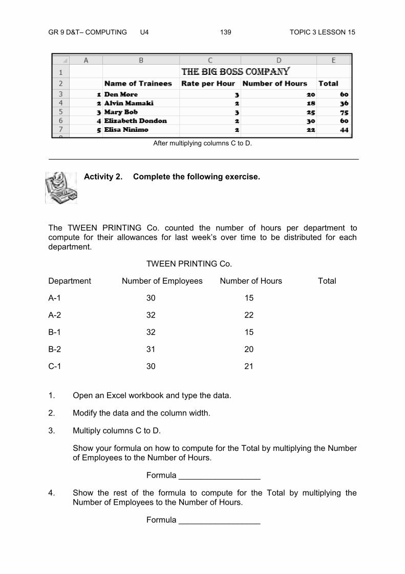
GR 9 D&T– COMPUTING U4 139 TOPIC 3 LESSON 15
After multiplying columns C to D.
Activity 2. Complete the following exercise.
The TWEEN PRINTING Co. counted the number of hours per department to compute for their allowances for last week’s over time to be distributed for each department.
TWEEN PRINTING Co.
Department Number of Employees Number of Hours Total
A-1 30 15
A-2 32 22
B-1 32 15
B-2 31 20
C-1 30 21
1. Open an Excel workbook and type the data.
2. Modify the data and the column width.
3. Multiply columns C to D.
Show your formula on how to compute for the Total by multiplying the Number of Employees to the Number of Hours.
Formula __________________
4. Show the rest of the formula to compute for the Total by multiplying the Number of Employees to the Number of Hours.
Formula __________________

GR 9 D&T– COMPUTING U4 140 TOPIC 3 LESSON 15
Formula __________________ Formula __________________
Formula __________________
5. Write your formula for the Total.
Total _____________________
Total _____________________
Total _____________________
Total _____________________
Total _____________________
6. Save your work with the filename Multiply2.
Thank you for completing this activity. Now, you may go to the end of this lesson to check your answer. Make sure you do the necessary corrections before moving on to the next part of this lesson.
Summary
You have come to the end of Lesson 15. In this lesson you learnt how to multiply numbers in various cells.
NOW DO PRACTICE EXERCISE 15 ON THE NEXT PAGE.

GR 9 D&T– COMPUTING U4 141 TOPIC 3 LESSON 15
Practice Exercise: 15
__________________________________________________________________________________
A. Follow the instructions below.
1. Open an Excel workbook and type the given data.
Make a Multiplication Table Using Excel for the given numbers.
1 * 6
2 * 6
3 * 6
4 * 6
5 * 6
6 * 6
7 * 6
8 * 6
9 * 6
10* 6
2. Create your own Title for the given problem.
3. Use ROCKWELL EXTRA BOLD for the text and with the font size of 13.
4. Save your work with the filename Multiplication3.
Answers to the Activity:
3. Formula =C3*D3
4. Formula =C4*D4
=C5*D5
=C6*D6
=C7*D*
5. Answers to the Total 450
704
480
620
630
CHECK YOUR WORK. ANSWERS ARE AT THE END OF TOPIC 3.

GR 9 D&T– COMPUTING U4 142 TOPIC 3 LESSON 16
Lesson 16: Dividing Numbers in Various Cells
_________________________________________________________________________
Welcome to lesson 16 of Unit 4. In Lesson 15, you learnt how to multiply numbers in various cell references.
In this lesson you will be able to divide two numbers in various cell references.
Your Aims: identify the process of dividing two numbers in
various cells
divide two numbers in various cells _________________________________________________________________________
Division of two Numbers in Various Cells
Microsoft Office Excel is a very popular application for spreadsheet management. One of its strength lies in Formulas and Functions. They let you perform basic calculations within Excel spreadsheets.
Remember that the symbol for our division in Excel is a forward slash ( / ) symbol.
First let us recall our division terms.
In the expression a / b = c, a is called the dividend or numerator, b the divisor or denominator and the result c is called the quotient.
Division describes two distinct but related settings. Partitioning involves taking a set of size a and forming b groups that are equal in size. The size of each group formed, c, is the quotient of a and b.
Quantitative division involves taking a set of size a and forming groups of size c. The number of groups of this size that can be formed, b, is the quotient of a and c.
Even though you can use numbers directly in your division formula, it is much better to use the references or addresses of the cells containing your data. If you use the cell references rather than the actual data later or if you need to change the data in either cell, the results of the formula will update automatically without you having to rewrite the formula.
Let us divide the two numbers:
C = 25 / 5 1. Let us use our Excel to type these two numbers.
A1 Dividend
B1 Divisor
C1 Quotient

GR 9 D&T– COMPUTING U4 143 TOPIC 3 LESSON 16
A2 25
B2 5
2. Place our active cell in C2 to write our answer (quotient).
3. Write your formula for dividing two numbers in division.
= A2 / B2
4. Type our formula in our formula bar.
5. Press Enter.
Your screen should look like this after typing the formula for division.
6. Save your work with the filename Division1.
Activity 1. Follow the given instructions below.
A. Melissa made 324 cupcakes. She packed 4 cupcakes into each box. How many boxes of cupcakes did she pack?
______________________________________________________________
______________________________________________________________

GR 9 D&T– COMPUTING U4 144 TOPIC 3 LESSON 16
1. Make a table in Excel on how to get the quotient to this problem.
2. Modify the text and the column.
3. Save your work with the filename Division 2.
B. In July, a construction company built a 360 mile road. In February the same company laid down 60 miles of road. How many times more roads did the company complete in July?
1. Make a table in Excel on how to get the quotient to this problem.
2. Modify the text and the column.
3. Save your work with the filename Division 3.
Thank you for completing this activity. Now, you may go to the end of this lesson to check your answer. Make sure you do the necessary corrections before moving on to the next part of this lesson.
Summary
You have come to the end of Lesson 16. In this lesson you learnt to divide two numbers in various cells.
NOW DO PRACTICE EXERCISE 16 ON THE NEXT PAGE.

GR 9 D&T– COMPUTING U4 145 TOPIC 3 LESSON 16
Practice Exercise: 16
___________________________________________________________________
A. Follow the given instructions to complete the exercise.
1. The National Capital District Commission (NCDC) decided to give new rubbish bins to every school in NCD. The Director of the District Commission requested every school to write a request letter for this.
The National Capital District Commission will give out 50 rubbish bins to distribute equally to schools.
Here is the list of school that replied to the NCDC’s request.
1. Gordon Secondary School
2. Kila Kila Secondary School
3. Gerehu Secondary School
4. Coronation Primary School
5. Koroboro School
6. Port Moresby Grammar School
7. St. Joseph School
8. Wardstrip School
9. Paradise School
Compute for the number of rubbish bins each school will receive.
2. A private sector group decided to help the country that was affected by the natural disasters last month. They decided to give sacks of rice to the six areas that were affected by the floods.
Areas Affected Sacks of Rice per Area Villages in a District
1 84 2
2 90 5
3 60 10
4 36 6
5 100 5
6 49 7
Compute for the number of sacks of rice to be distributed per village.
CHECK YOUR WORK. ANSWERS ARE AT THE END OF TOPIC 3.
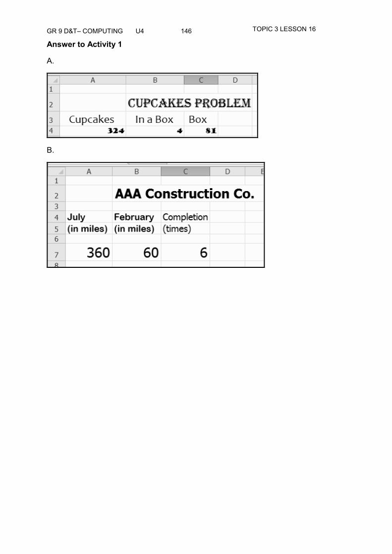
GR 9 D&T– COMPUTING U4 146 TOPIC 3 LESSON 17
TOPIC 3 LESSON 16
Answer to Activity 1
A.
B.

GR 9 D&T– COMPUTING U4 147 TOPIC 3 LESSON 17
Lesson 17: Using Auto Sum
_________________________________________________________________________
Welcome to lesson 17 of Unit 4. In Lesson 16, you learnt how to divide two numbers in various cell references.
In this lesson you will be able to define Auto Sum, identify its purpose, identify the steps for using Auto Sum, use Auto Sum to add numbers in various cells and state the benefits gained in using Auto Sum in a Spreadsheet.
Your Aims: define Auto Sum
identify how to use Auto Sum
add consecutive list of numbers __________________________________________________________________________
AutoSum
First, let us define Auto Sum. AutoSum is a shortcut for the SUM Function.
A function in a Spreadsheet program which inserts a formula in the selected cell that adds the numbers in the column above it. It sets the range of cells by looking for numeric data above the selected cell.
The Auto Sum button, located on the Standard Toolbar in Excel 2010, is a shortcut provided for using the SUM function. When you click on the Auto Sum button, the SUM function is entered into the active cell.
Let us consider our sample worksheet in Lesson 13 with the filename Addition2.
Auto Sum

GR 9 D&T– COMPUTING U4 148 TOPIC 3 LESSON 17
Let us delete the answers for the TOTAL (I4 to I10) and Days Total (B10 to B9).
1. Highlight the cell references that we wanted to delete.
2. Click the Delete button located at the Standard Toolbar and click the down arrow to show you more of the delete commands.
3. Choose Delete Sheet Columns to delete the highlighted columns.

GR 9 D&T– COMPUTING U4 149 TOPIC 3 LESSON 17
4. Do the same for cell references B10 to H10 (go back to step 1). As you notice when we deleted the columns the titles for Column I were deleted as well (Total), the same with the row (Days Total).
5. Create another title for A11 which is Daily Total and for cell reference J3 type Weekly Total.
To use the Auto Sum Button Follow the instructions below on how to use the Auto Sum button.
1. Click on the cell where you want the answer to appear.
2. Click on the Auto Sum button .
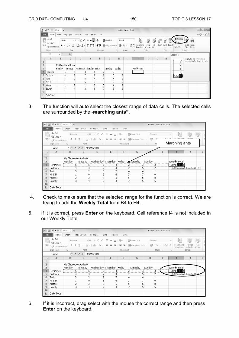
GR 9 D&T– COMPUTING U4 150 TOPIC 3 LESSON 17
3. The function will auto select the closest range of data cells. The selected cells are surrounded by the ―marching ants”.
4. Check to make sure that the selected range for the function is correct. We are trying to add the Weekly Total from B4 to H4.
5. If it is correct, press Enter on the keyboard. Cell reference I4 is not included in our Weekly Total.
6. If it is incorrect, drag select with the mouse the correct range and then press Enter on the keyboard.
Marching ants

GR 9 D&T– COMPUTING U4 151 TOPIC 3 LESSON 17
7. Press Enter.
8. Do the same for columns J5, J6, J7, J8 and J9.
9. Compute for the Daily Total using the Auto Sum (Refer to Step 1). This is how your screen should look like after using the Auto Sum.
Drag your mouse to your right.
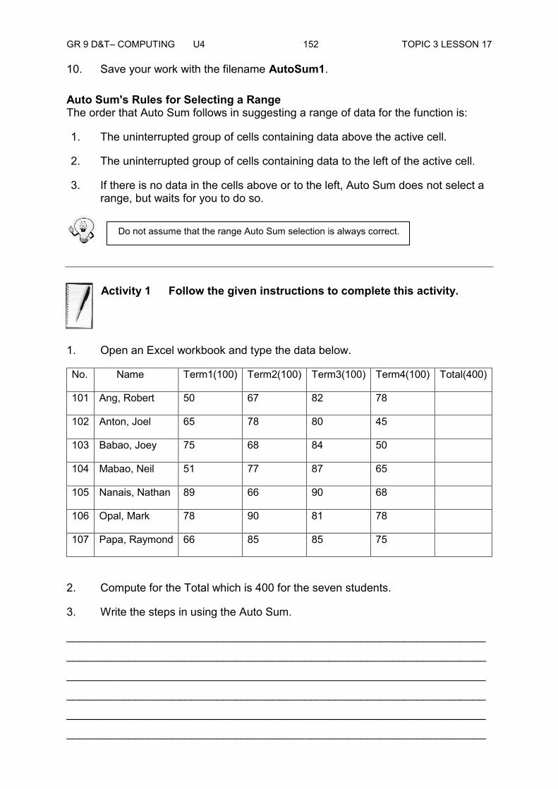
GR 9 D&T– COMPUTING U4 152 TOPIC 3 LESSON 17
Do not assume that the range Auto Sum selection is always correct.
10. Save your work with the filename AutoSum1.
Auto Sum's Rules for Selecting a Range The order that Auto Sum follows in suggesting a range of data for the function is:
1. The uninterrupted group of cells containing data above the active cell.
2. The uninterrupted group of cells containing data to the left of the active cell.
3. If there is no data in the cells above or to the left, Auto Sum does not select a range, but waits for you to do so.
Activity 1 Follow the given instructions to complete this activity.
1. Open an Excel workbook and type the data below.
No. Name Term1(100) Term2(100) Term3(100) Term4(100) Total(400)
101 Ang, Robert 50 67 82 78
102 Anton, Joel 65 78 80 45
103 Babao, Joey 75 68 84 50
104 Mabao, Neil 51 77 87 65
105 Nanais, Nathan 89 66 90 68
106 Opal, Mark 78 90 81 78
107 Papa, Raymond 66 85 85 75
2. Compute for the Total which is 400 for the seven students.
3. Write the steps in using the Auto Sum.
___________________________________________________________________
___________________________________________________________________
___________________________________________________________________
___________________________________________________________________
___________________________________________________________________
___________________________________________________________________

GR 9 D&T– COMPUTING U4 153 TOPIC 3 LESSON 17
4. Save your work with the filename AutoSum2.
Thank you for completing this activity. Now, you may go to the end of this lesson to check your answer. Make sure you do the necessary corrections before moving on to the next part of this lesson.
Summary
You have come to the end of Lesson 17. In this lesson you learnt how to use the Auto Sum and to add consecutive list of numbers using the Auto Sum.
NOW DO PRACTICAL EXERCISE 17 ON THE NEXT PAGE.
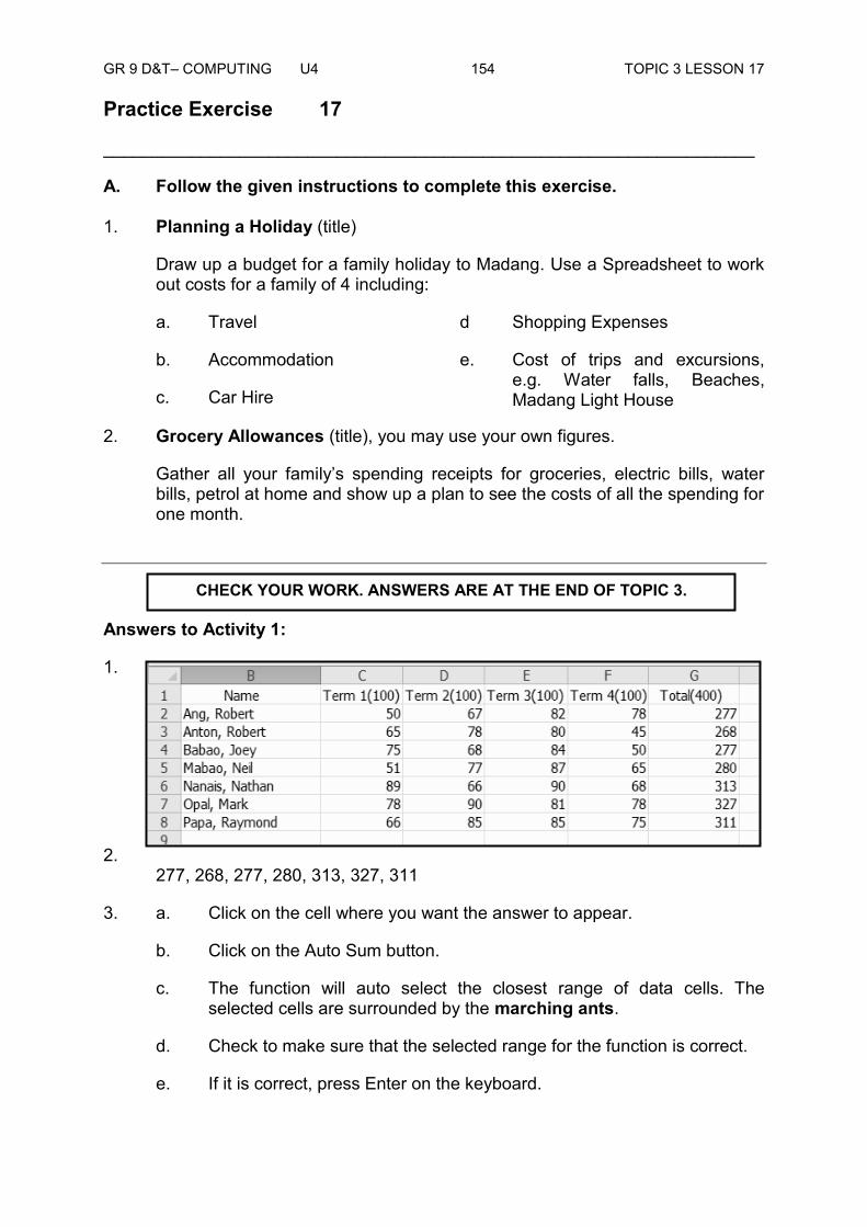
GR 9 D&T– COMPUTING U4 154 TOPIC 3 LESSON 17
Practice Exercise 17
___________________________________________________________________
A. Follow the given instructions to complete this exercise.
1. Planning a Holiday (title)
Draw up a budget for a family holiday to Madang. Use a Spreadsheet to work out costs for a family of 4 including:
a. Travel
b. Accommodation
c. Car Hire
d Shopping Expenses
e. Cost of trips and excursions, e.g. Water falls, Beaches, Madang Light House
2. Grocery Allowances (title), you may use your own figures.
Gather all your family’s spending receipts for groceries, electric bills, water bills, petrol at home and show up a plan to see the costs of all the spending for one month.
Answers to Activity 1:
1.
2. 277, 268, 277, 280, 313, 327, 311
3. a. Click on the cell where you want the answer to appear.
b. Click on the Auto Sum button.
c. The function will auto select the closest range of data cells. The selected cells are surrounded by the marching ants.
d. Check to make sure that the selected range for the function is correct.
e. If it is correct, press Enter on the keyboard.
CHECK YOUR WORK. ANSWERS ARE AT THE END OF TOPIC 3.

GR 9 D&T– COMPUTING U4 155 TOPIC 3 LESSON 17
f. If it is incorrect, drag select with the mouse the correct range and then
press Enter on the keyboard. g. Press Enter. h. Do the same for the rest of the columns.
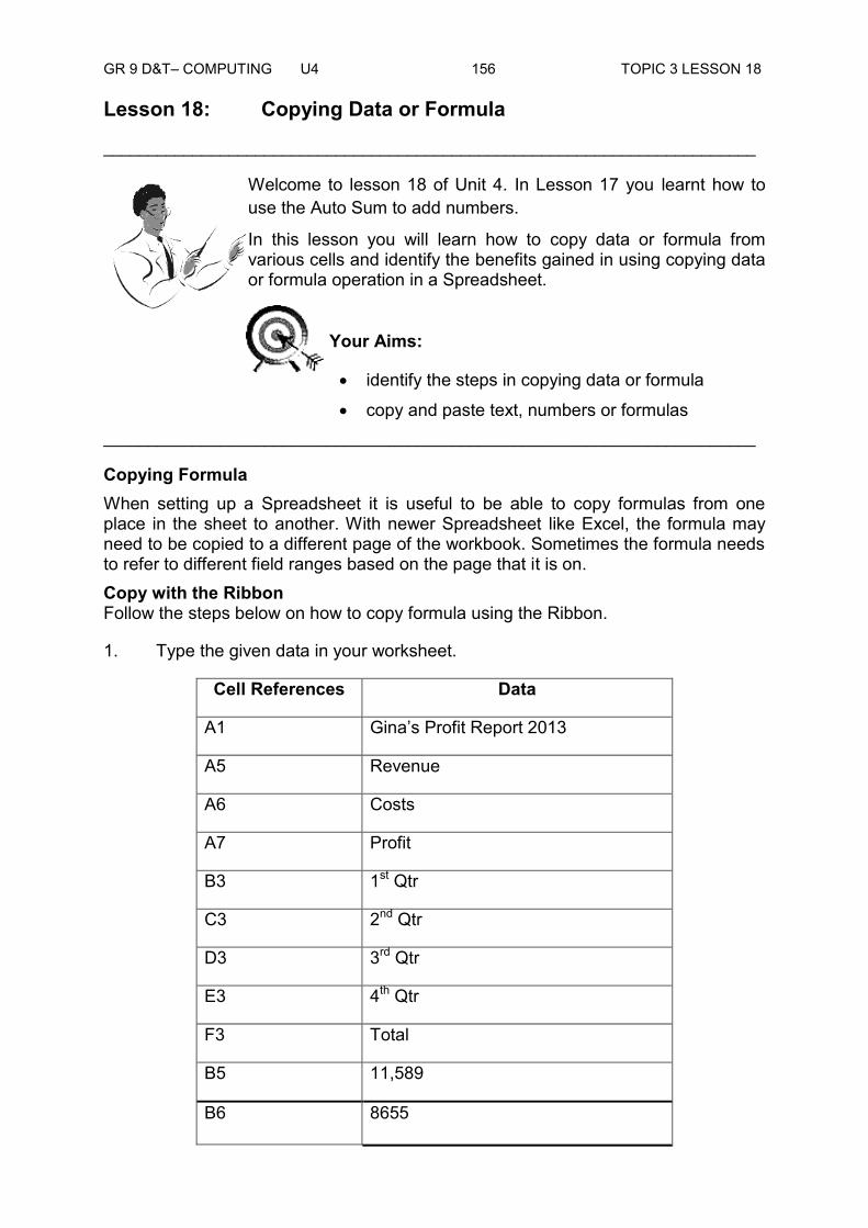
GR 9 D&T– COMPUTING U4 156 TOPIC 3 LESSON 18
Lesson 18: Copying Data or Formula
_________________________________________________________________________
Welcome to lesson 18 of Unit 4. In Lesson 17 you learnt how to use the Auto Sum to add numbers.
In this lesson you will learn how to copy data or formula from various cells and identify the benefits gained in using copying data or formula operation in a Spreadsheet.
Your Aims:
identify the steps in copying data or formula
copy and paste text, numbers or formulas _________________________________________________________________________
Copying Formula When setting up a Spreadsheet it is useful to be able to copy formulas from one place in the sheet to another. With newer Spreadsheet like Excel, the formula may need to be copied to a different page of the workbook. Sometimes the formula needs to refer to different field ranges based on the page that it is on. Copy with the Ribbon Follow the steps below on how to copy formula using the Ribbon.
1. Type the given data in your worksheet.
Cell References Data
A1 Gina’s Profit Report 2013
A5 Revenue
A6 Costs
A7 Profit
B3 1st Qtr
C3 2nd Qtr
D3 3rd Qtr
E3 4th Qtr
F3 Total
B5 11,589
B6 8655

GR 9 D&T– COMPUTING U4 157 TOPIC 3 LESSON 18
B7 3501
C5 14500
C6 9620
C7 3562
D5 11600
D6 9621
D7 3057
E5 13333
E6 10555
E7 2336
This is how your data will look like in Excel.
2. Compute for the Total using the Auto Sum (Refer to Lesson 17).
After computing the Total

GR 9 D&T– COMPUTING U4 158 TOPIC 3 LESSON 18
3. Place your active cell to F5 (the cell reference or formula) that we want to
copy. 4. Choose Home Tab. 5. Click the Copy button in the Clipboard group, the Excel copies the
formula in cell F5.
6. As soon you click the Copy button for the cell reference F5, the cell will have marching ants’ border.
7. Press the right arrow key of your mouse once to move to cell G5 (where we will copy the formula).

GR 9 D&T– COMPUTING U4 159 TOPIC 3 LESSON 18
8. Click the left button of your mouse to remove the Context Menu and the Mini
toolbar. 9. As you will notice the marching ants are in F5 and the active cell is in G5. 10. Click the Paste button. Excel pastes the formula in cell F5 into cell
G5.
Compare the formula in cell F5 with the formula in cell G5 (while in the respective cell, look at the Formula bar). The formulas are the same except that the formula in cell F5 sums the entries in Column F and the formula in cell G5 sums the entries in column G. The formula was copied in a relative fashion.
Before proceeding with the next part of the exercise, you must copy the information in cells F6 to G6 to cells F7 to G7.
This is how your sheet should look like after copying the formula. Copy with the Mini Toolbar This time you will copy using the Mini toolbar. Follow the steps below on how to copy formula using the Mini Toolbar.
1. Select cells B5 to G5.
2. Move to cell B5.
3. Press the Shift Key. While holding down the Shift Key, press the arrow right key five times (from columns C, D, E, F,G).
4. Press the right arrow key once. Excel highlights B5 to G5.

GR 9 D&T– COMPUTING U4 160 TOPIC 3 LESSON 18
5. Right click your mouse. A Context Menu and a Mini toolbar will appear.
6. Click Copy, which is located on the context menu. Excel copies the information in cells G5 to H5.
7. After clicking the Copy button, cell references B5 to G5 aside from being
highlighted it will have marching ants, place your active cell to B9 to copy.
8. Right click your mouse to appear the context menu. Select Paste button to copy the selected cell refences to B9

GR 9 D&T– COMPUTING U4 161 TOPIC 3 LESSON 18
9. Click Paste. Excel copies the contents of cells B5 to G5 to cells B9 to G9.
10. Press Esc to exit Copy mode.
11. Do the same to Costs to cell references B10 to G10 and Profit to cell references to B11 to G11. This is how your worksheet should look like after after copying using the Mini toolbar.
GR 9 D&T– COMPUTING U4 162 TOPIC 3 LESSON 18
12. Save yourwork with the filename Minitoolbar1.
___________________________________________________________________
Activity 1. Answer the following.
A. Discuss the steps on how to copy formula using the Ribbon.
___________________________________________________________________
___________________________________________________________________
___________________________________________________________________
___________________________________________________________________
___________________________________________________________________
___________________________________________________________________
___________________________________________________________________
B. Discuss the steps on how to copy/paste using the Mini tool bar menu.
___________________________________________________________________
___________________________________________________________________
___________________________________________________________________
___________________________________________________________________
___________________________________________________________________
___________________________________________________________________
___________________________________________________________________
Thank you for completing this activity. Now, you may go to the end of this lesson to check your answer. Make sure you do the necessary corrections before moving on to the next part of this lesson.
Summary
You have come to the end of Lesson 18. In this lesson you learnt how to use the Ribbon and the Mini toolbar to Copy and Paste certain formulas and contents.
NOW DO PRACTICE EXERCISE 18 ON THE NEXT PAGE.
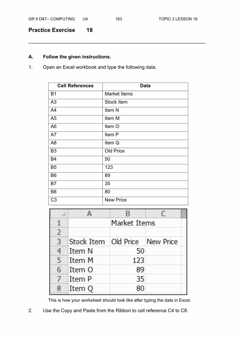
GR 9 D&T– COMPUTING U4 163 TOPIC 3 LESSON 18
Practice Exercise 18
__________________________________________________________________
A. Follow the given instructions.
1. Open an Excel workbook and type the following data.
Cell References Data B1 Market Items
A3 Stock Item
A4 Item N
A5 Item M
A6 Item O
A7 Item P
A8 Item Q
B3 Old Price
B4 50
B5 123
B6 89
B7 35
B8 80
C3 New Price
This is how your worksheet should look like after typing the data in Excel.
2. Use the Copy and Paste from the Ribbon to cell reference C4 to C8.

GR 9 D&T– COMPUTING U4 164 TOPIC 3 LESSON 18
B. From Practice Exercise 18.1. 1. Add another cell which is in D3 and type Price 2013.
2. Use addition method to add Old Price and the New Price to cell references D4 to D8 (Price 2013).
3. Type Price 2014 to E3.
4. Use Mini toolbar to compute for Price 2014 by adding cell references C3 and D3.
Answers to the Activity:
1. Steps on how to copy formula using the Ribbon. a. Place your active cell to a cell (the cell reference or formula) that we
want to copy.
b. Choose Home Tab.
c. Click the Copy button in the Clipboard group, the Excel copies the formula in the cell.
d. As soon you click the Copy button for the cell reference, the cell will have marching ants’ border.
e. Press the right arrow key of your mouse once to move to cell (where we will copy the formula).
f. Click the left button of your mouse to remove the Context Menu and the Mini toolbar.
g. As you will notice the marching ants are in old cell and the active cell is in the target cell to copy.
h. Click the Paste button in the Clipboard group.
CHECK YOUR WORK. ANSWERS ARE AT THE END OF TOPIC 3.

GR 9 D&T– COMPUTING U4 165 TOPIC 3 LESSON 18
2. Steps on how to copy/paste using the Mini tool bar menu a. Select cells to copy.
b. Press the Shift Key. While holding down the Shift Key, press the arrow right key depending on how many cells you will copy.
c. Right click your mouse. A Context Menu and a Mini toolbar will appear.
d. Click Copy, which is located on the context menu. Excel copies the information in the cells.
e. After clicking the Copy button, cell references will be highlighted and it will have marching ants. Place your active cell to the cell you want to copy the content.
f. Right click your mouse to appear the context menu. Select Paste button to copy the selected cell refences.
g. Press Esc to exit Copy mode.
h. Do the same to other cell references that need to be copied.
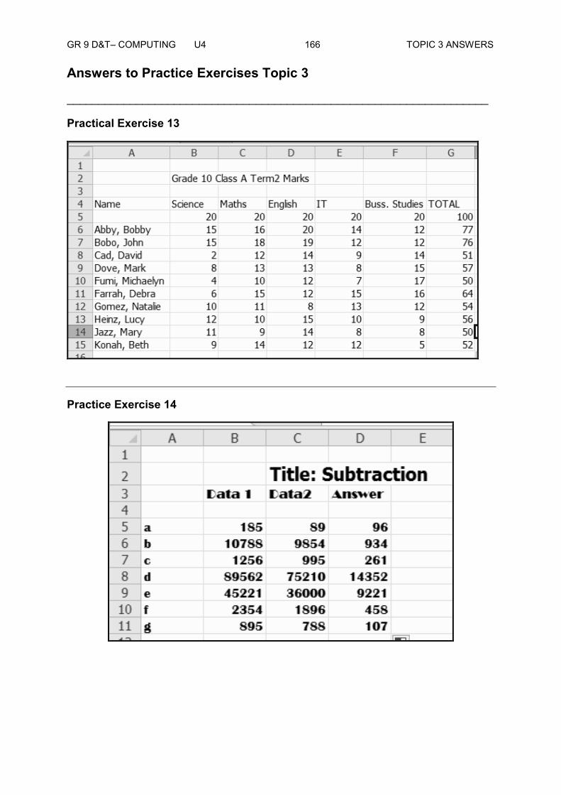
GR 9 D&T– COMPUTING U4 166 TOPIC 3 ANSWERS
Answers to Practice Exercises Topic 3
___________________________________________________________________
Practical Exercise 13
Practice Exercise 14

GR 9 D&T– COMPUTING U4 167 TOPIC 3 ANSWERS
Practice Exercise 15
Practice Exercise 16
a.
b.
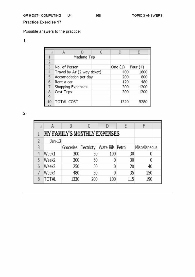
GR 9 D&T– COMPUTING U4 168 TOPIC 3 ANSWERS
Practice Exercise 17
Possible answers to the practice:
1.
2.

GR 9 D&T– COMPUTING U4 169 TOPIC 3 ANSWERS
Practice Exercise 18 1.
2.
End of Topic 3
Now Do Exercise 3 in Assignment Book 3 Then Go to Topic 4.

GR 9 D&T– COMPUTING U4 170 TOPIC 3 ANSWERS
TOPIC TITLE
TOPIC 4
DOING MORE WITH SPREADSHEET
Lesson 19 : Creating a More Complex or Unusual Formula
Lesson 20 : Formatting a Worksheet Lesson 21 : Using Print Preview Lesson 22 : Printing A Worksheet Lesson 23 : Creating A Graph with Chart Wizard Lesson 24 : Incorporating Graphs in Word
Processing

GR 9 D&T– COMPUTING U4 171 TOPIC INTRODUCTION
TOPIC 4: DOING MORE WITH SPREADSHEET
___________________________________________________________________
In this topic you will learn about creating a more complex or unusual formula, formatting a worksheet, using print preview, printing a worksheet, creating a graph with chart wizard and incorporating graphs in word processing.
With Excel you can analyse, manage and share information quickly and easily to make more informed decisions. With the new user interface, rich data visualization, and PivotTable views, professional-looking charts are easier to create and use than ever before.
In this topic you will study the following:
Lesson 19 discusses on creating a more complex or unusual formula. You will learn how to create it and the benefits of creating a more complex or unusual formula.
Lesson 20 explains how to format a worksheet. You will learn the meaning of worksheets, how to format a worksheet and the benefits of using a worksheet.
Lesson 21 focuses on the uses of print preview. You will learn about print preview, how to use print preview before printing.
Lesson 22 discusses on printing a worksheet. You will learn the things to consider before printing a worksheet; explain the benefits of printing a worksheet and how to print a worksheet.
Lesson 23 explains creating a graph with chart wizard. You will learn about the chart wizard and its purpose, locate chart wizard from the computer menu, enumerate and explain its features, decide the appropriate graph for a given data and how to create a graph using the chart wizard.
Lesson 24 focuses on incorporating graphs in word processing. You will learn how to transfer, add, combine or incorporate Excel graphs in word document and enumerate specific items to consider in incorporating Excel graphs in word document.
By the end of Topic 4, you should be able to use the complex formula, format a worksheet, use the print preview, print a worksheet, create graphs using a chart wizard and incorporate graphs into word processing.

GR 9 D&T– COMPUTING U4 172 TOPIC 4 LESSON 19
Lesson 19: Creating a More Complex or Unusual Formula
_______________________________________________________________________
Welcome to Lesson 19 of Unit 4. In Lesson 18, you learnt how to copy data or formula. In this lesson you will learn about complex or unusual formula, how to create it and its benefits.
Your Aims:
_________________________________________________________________________
Complex Formula First let us define complex formula: Simple formulas have one mathematical operation. Complex formulas involve more than one mathematical operation. Simple Formula: =2+2 Complex Formula: =2+2*8
To calculate complex formulas correctly, you must perform certain operations before others. This is defined in the order of operations.
Complex formula allows the Excel user to manipulate more numbers for data interpretation. It provides the user flexibility to manipulate operations as needed in any data evaluation done in Excel.
The Order of Operations The order of mathematical operations is very important. If you enter a formula that contains several operations, Excel knows how to work those operations in a specific order. The order of operations is:
Operations enclosed in parenthesis ( )
Exponential calculations (to the power of)
Multiplication and division, whichever comes first
Addition and subtraction, whichever comes first
A mnemonic that can help you remember this is Please Excuse My Dear Aunt Sally (P.E.M.D.A.S).
P for parenthesis
E for exponential
M for multiplication
D for division
define complex or unusual formula identify the steps on how to create complex or
unusual formula create a formula that contains a function
GR 9 D&T– COMPUTING U4 173 TOPIC 4 LESSON 19
A for addition
S for subtraction
Example 1
4+4*3=?
Is the answer 16 or 24? Well, if you calculated in the order in which the numbers appear, 4+4*3, you'd get the wrong answer, 24. You must follow the order of operations to get the correct answer. To Calculate the Correct Answer Calculate 4*3 first because multiplication comes before addition in the order of operations. The answer is 16.
Add the answer obtained in step #1, which is 12, to the number 4 that opened the equation. In other words, add 4 + 12.
The answer is 16.
Example 2
30 / ( 6 – 3 ) * 6 - 3
Using this order, let us see how the formula 30/(6-3)*6-3 is calculated in the following breakdown:
30 / ( 6 – 3 ) * 6 - 3 Perform the operations in parenthesis first
( 6 – 3 ) = 3
30 / 3 * 6 – 3 Because the division comes first before the multiplication, divide 30 / 3 = 10
10 * 6 – 3 Next is, multiplication takes place before the subtraction 10 * 6 = 60
10 – 3 Formula becomes, 60 – 3, and the final answer is 57
Other Complex Formulas Excel automatically follows a standard order of operations in a complex formula. If you want a certain portion of the formula to be calculated first, put it in parentheses. Let us have more sample formulas to make sure you understand the order of operations by which Excel calculates the answer.
4*2/4 (4*2)/4
Multiply 4*2 before performing the division operation because the multiplication sign comes before the division sign. The answer is 2.
4/2*4 (4/2)*4

GR 9 D&T– COMPUTING U4 174 TOPIC 4 LESSON 19
Divide 4 by 2 before performing the multiplication operation because the division sign comes before the multiplication sign. The answer is 8.
4-2*4 4-(2*4)
Multiply 2*4 before performing the subtraction operation because the multiplication sign is of a higher order than the subtraction sign. The answer is -4.
4/(2*4)
But if the given complex formula is with the parenthesis, perform the operation in parentheses (2*4) first and divide 4 by this result. The answer is 0.5.
___________________________________________________________________ Activity 1: Follow the given instructions.
A. Compute using the order of Mathematical Operations
1. 81 / 9 – 7 * 3 + 20
2. 100 – 5 * 20 / 2 + 6
3. 70 – 2 * 6 / 2 + 4
4. 92 + 2 * 5 / 10
5. 6 * 3 / 2 + 2 – 6
B. What is the importance of using complex formula?
___________________________________________________________________
___________________________________________________________________
___________________________________________________________________
Thank you for completing this activity. Now, you may go to the end of this lesson to check your answer. Make sure you do the necessary corrections before moving on to the next part of this lesson.
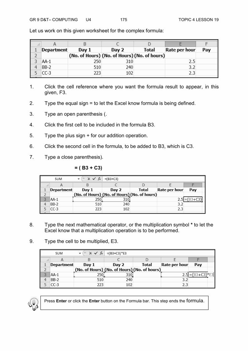
GR 9 D&T– COMPUTING U4 175 TOPIC 4 LESSON 19
Let us work on this given worksheet for the complex formula:
1. Click the cell reference where you want the formula result to appear, in this
given, F3.
2. Type the equal sign = to let the Excel know formula is being defined.
3. Type an open parenthesis (.
4. Click the first cell to be included in the formula B3.
5. Type the plus sign + for our addition operation.
6. Click the second cell in the formula, to be added to B3, which is C3.
7. Type a close parenthesis).
= ( B3 + C3)
8. Type the next mathematical operator, or the multiplication symbol * to let the Excel know that a multiplication operation is to be performed.
9. Type the cell to be multiplied, E3.
Press Enter or click the Enter button on the Formula bar. This step ends the formula.

GR 9 D&T– COMPUTING U4 176 TOPIC 4 LESSON 19
10. Now continue for F4 and F5 by going back to our step 1.
After following the steps 1 to 9.
Activity 2. Follow the given instructions.
1. Give the order of operations in complex or unusual formula.
a. ______________
b. _______________
c. _______________
d. _______________
e. _______________
f. _______________
2. List the mnemonic to help you remember the order of operations.
a. ______________
b. ______________
c. ______________
d. ______________
e. ______________
f. ______________
3. Write the order of operations from the given complex formula.
100 – 6 * 3 / 9 * 2 – 10
______________________________________________________________
______________________________________________________________
______________________________________________________________
Write your final answer here ___________________________

GR 9 D&T– COMPUTING U4 177 TOPIC 4 LESSON 19
Thank you for completing this activity. Now, you may go to the end of this lesson to check your answer. Make sure you do the necessary corrections before moving on to the next part of this lesson.
Summary
You have come to the end of Lesson 19. In this lesson you learnt how to compute using the complex or unusual formula
NOW DO PRACTICE EXERCISE 19 ON THE NEXT PAGE.

GR 9 D&T– COMPUTING U4 178 TOPIC 4 LESSON 19
Practice Exercise: 19
__________________________________________________________________
A. Follow the given instructions. 1. Type and solve for the answers using complex or unusual formula.
When you create your formula, write the cell references for each number. (e. g. = A1 + B1)
Given: A1 – 3 B1 – 5 C1 – 12 D1 – 2 E1 – 4
a. 3 + 5 + 12 / 2 * 4 your answer in cell A3
b. ( 3 + 5 + 12 ) / 2 * 4 your answer in cell A5
c. 3 + ( 5 + ( 12 / 2 )) * 4 your answer in cell A7
d. 3 + 5 + ( 12 / 2 * 4 ) your answer in cell A9
e. 3 + ( 5 + ( 12 / 2 * 4 )) your answer in cell A11
Answers to Activities A. 1. 81 / 9 – 7 * 3 + 20 (81 / 9) – (7 * 3) + 20 (81 / 9) – 21 + 20 9 – (21 + 20) 9 – 1 8 2. 100 – 5 * 20 / 2 + 6 100 – (5 * 20) / 2 + 6 100 – (100 / 2) + 6 100 – (50 + 6) 100 – 56 44 3. 70 – 2 * 6 / 2 + 4 70 – (2 * 6) / 2 + 4
70 – (12 / 2) + 4 70 – (6 + 4) 60 4. 92 + 2 * 5 / 10 92 + (2 * 5) / 10 92 + (10 / 10) 93 5. 6 * 3 / 2 + 2 – 6 (6 * 3) / 2 + 2 – 6 (18 / 2) + 2 – 6 (9 +2) – 6 11 – 6 5
CHECK YOUR WORK. ANSWERS ARE AT THE END OF TOPIC 4.

GR 9 D&T– COMPUTING U4 179 TOPIC 4 LESSON 19
B. Complex formula allows the Excel user to manipulate more numbers for data interpretation. It provides the user flexibility to manipulate operations as needed in any data evaluation done in Excel.
Activity 2 1. The Order of Operations
a. Operations enclosed in parenthesis ( )
b. Exponential calculations (to the power of)
c. Multiplication
d. Division
e. Addition
f. Subtraction
2. That mnemonic that can help you remember the complex operation Please Excuse My Dear Aunt Sally (P.E.M.D.A.S).
a. P for parenthesis
b. E for exponential
c. M for multiplication
d. D for division
e. A for addition
f. S for subtraction
3. 100 – 6 * 3 / 9 * 2 – 10
100 - ( 6 * 3 ) / 9 * 2 – 10………100 - 18 / 9 * 2 – 10
100 - (18 / 9) * 2 – 10 ………….100 - 2 * 2 – 10
100 - ( 2 * 2 ) – 10………………100 - 4 – 10
96 – 10
Final answer is 86.
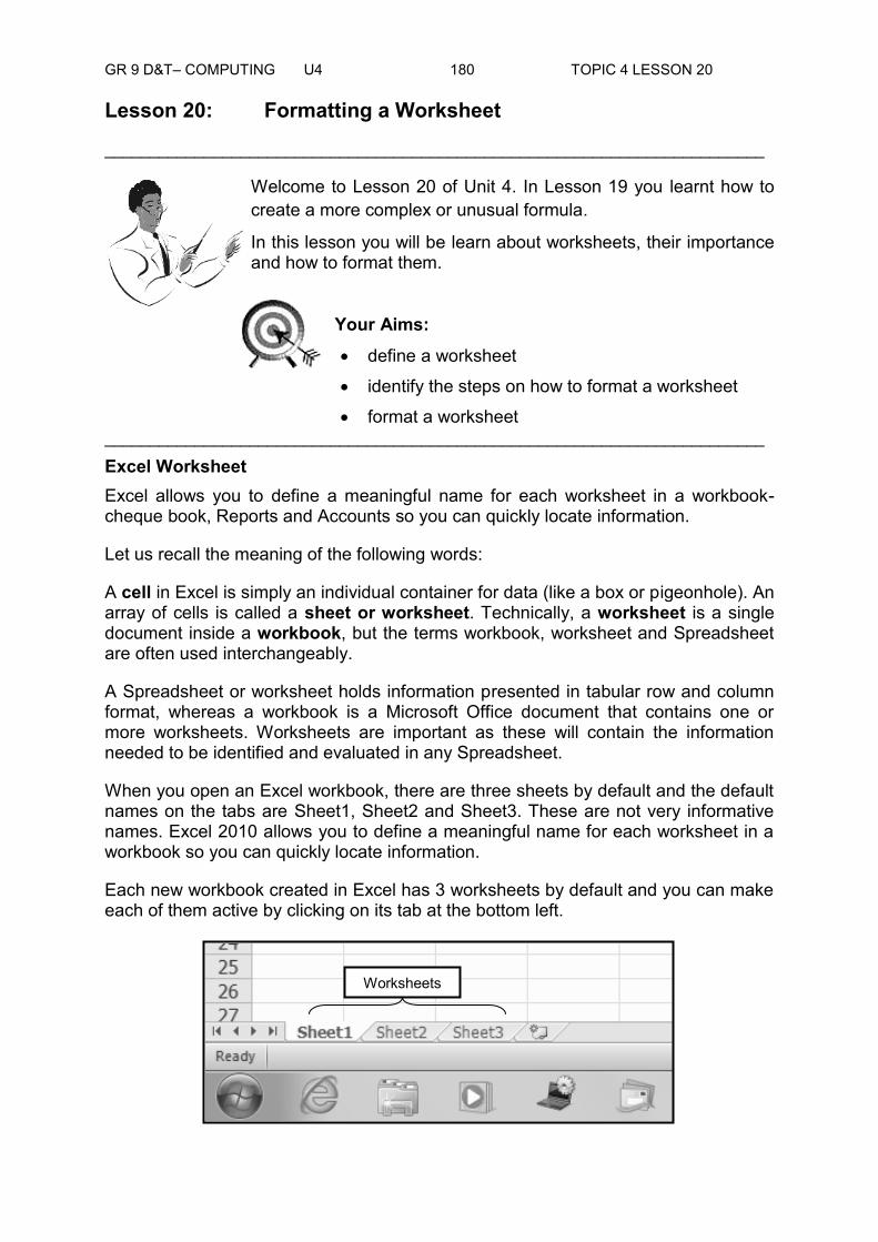
GR 9 D&T– COMPUTING U4 180 TOPIC 4 LESSON 20
Lesson 20: Formatting a Worksheet
_________________________________________________________________________
Welcome to Lesson 20 of Unit 4. In Lesson 19 you learnt how to create a more complex or unusual formula.
In this lesson you will be learn about worksheets, their importance and how to format them.
Your Aims:
_________________________________________________________________________ Excel Worksheet Excel allows you to define a meaningful name for each worksheet in a workbook-cheque book, Reports and Accounts so you can quickly locate information.
Let us recall the meaning of the following words:
A cell in Excel is simply an individual container for data (like a box or pigeonhole). An array of cells is called a sheet or worksheet. Technically, a worksheet is a single document inside a workbook, but the terms workbook, worksheet and Spreadsheet are often used interchangeably.
A Spreadsheet or worksheet holds information presented in tabular row and column format, whereas a workbook is a Microsoft Office document that contains one or more worksheets. Worksheets are important as these will contain the information needed to be identified and evaluated in any Spreadsheet.
When you open an Excel workbook, there are three sheets by default and the default names on the tabs are Sheet1, Sheet2 and Sheet3. These are not very informative names. Excel 2010 allows you to define a meaningful name for each worksheet in a workbook so you can quickly locate information.
Each new workbook created in Excel has 3 worksheets by default and you can make each of them active by clicking on its tab at the bottom left.
define a worksheet
identify the steps on how to format a worksheet
format a worksheet
Worksheets
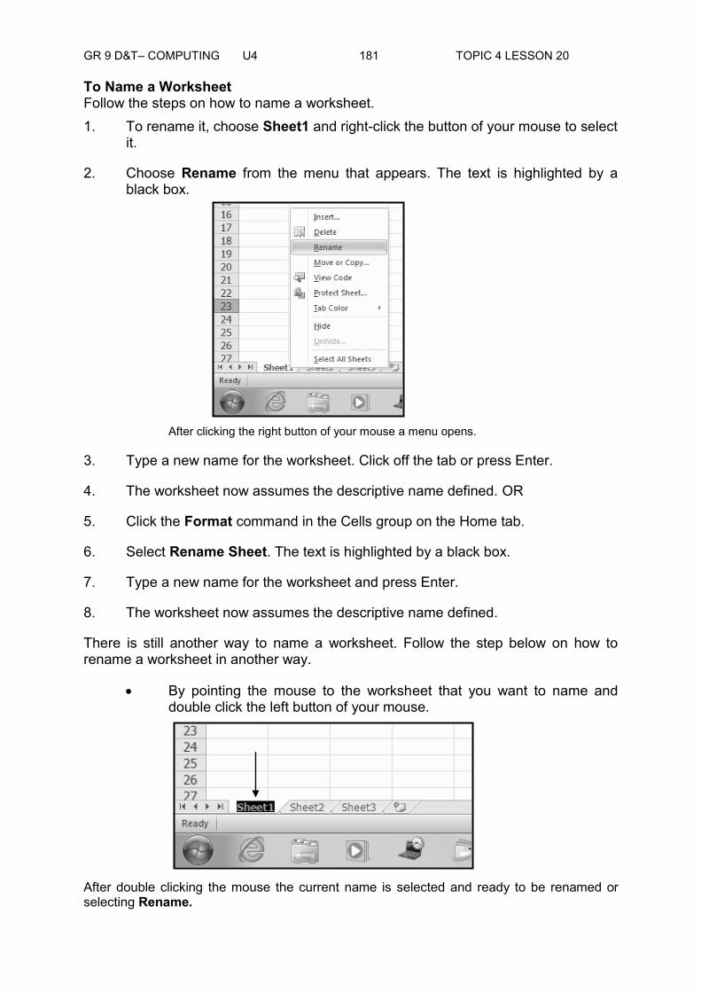
GR 9 D&T– COMPUTING U4 181 TOPIC 4 LESSON 20
To Name a Worksheet Follow the steps on how to name a worksheet. 1. To rename it, choose Sheet1 and right-click the button of your mouse to select
it.
2. Choose Rename from the menu that appears. The text is highlighted by a black box.
After clicking the right button of your mouse a menu opens.
3. Type a new name for the worksheet. Click off the tab or press Enter.
4. The worksheet now assumes the descriptive name defined. OR
5. Click the Format command in the Cells group on the Home tab.
6. Select Rename Sheet. The text is highlighted by a black box.
7. Type a new name for the worksheet and press Enter.
8. The worksheet now assumes the descriptive name defined.
There is still another way to name a worksheet. Follow the step below on how to rename a worksheet in another way.
By pointing the mouse to the worksheet that you want to name and double click the left button of your mouse.
After double clicking the mouse the current name is selected and ready to be renamed or selecting Rename.

GR 9 D&T– COMPUTING U4 182 TOPIC 4 LESSON 20
9. Suppose our first worksheet will be named Sample 1.
After naming worksheet as Sample1.
10. Continue to name the other two worksheets as Sample2 and Sample3.
After naming the three worksheets.
__________________________________________________________________________ Activity 1. Change the 6 worksheet names.
a. From Sheet1 to Activity1
b. From Sheet2 to Activity2
c. From Sheet3 to Activity3
d. From Sheet4 to Sample1
e. From Sheet5 to Sample2
f. From Sheet6 to Sample3
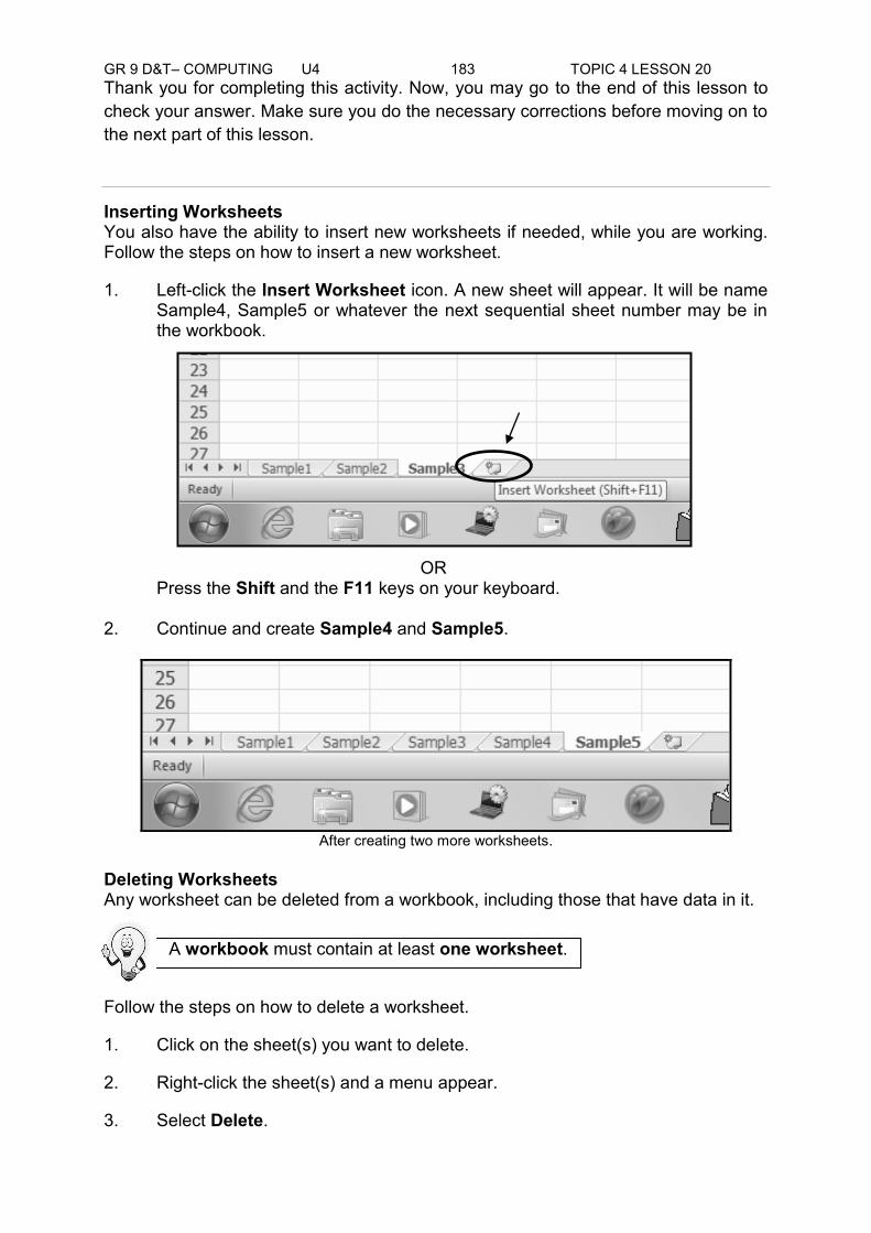
GR 9 D&T– COMPUTING U4 183 TOPIC 4 LESSON 20
Thank you for completing this activity. Now, you may go to the end of this lesson to check your answer. Make sure you do the necessary corrections before moving on to the next part of this lesson.
Inserting Worksheets You also have the ability to insert new worksheets if needed, while you are working. Follow the steps on how to insert a new worksheet.
1. Left-click the Insert Worksheet icon. A new sheet will appear. It will be name Sample4, Sample5 or whatever the next sequential sheet number may be in the workbook.
OR Press the Shift and the F11 keys on your keyboard.
2. Continue and create Sample4 and Sample5.
After creating two more worksheets.
Deleting Worksheets Any worksheet can be deleted from a workbook, including those that have data in it.
A workbook must contain at least one worksheet.
Follow the steps on how to delete a worksheet.
1. Click on the sheet(s) you want to delete.
2. Right-click the sheet(s) and a menu appear.
3. Select Delete.
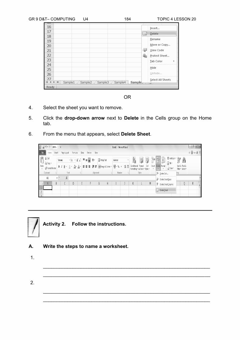
GR 9 D&T– COMPUTING U4 184 TOPIC 4 LESSON 20
OR
4. Select the sheet you want to remove.
5. Click the drop-down arrow next to Delete in the Cells group on the Home tab.
6. From the menu that appears, select Delete Sheet.
Activity 2. Follow the instructions.
A. Write the steps to name a worksheet. 1.
______________________________________________________________
______________________________________________________________
2.
______________________________________________________________
______________________________________________________________

GR 9 D&T– COMPUTING U4 185 TOPIC 4 LESSON 20
3.
______________________________________________________________
______________________________________________________________
4.
______________________________________________________________
______________________________________________________________
5.
______________________________________________________________
______________________________________________________________
6.
______________________________________________________________
______________________________________________________________
7.
______________________________________________________________
______________________________________________________________
8.
______________________________________________________________
______________________________________________________________
B. Write three steps to delete a worksheet 1.
______________________________________________________________
______________________________________________________________
2.
______________________________________________________________
______________________________________________________________
3.
______________________________________________________________
______________________________________________________________
C. Give the importance of worksheets in a Spreadsheet.
______________________________________________________________
______________________________________________________________

GR 9 D&T– COMPUTING U4 186 TOPIC 4 LESSON 20
Thank you for completing this activity. Now, you may go to the end of this lesson to check your answers. Make sure you do the necessary corrections before moving on to the next part of this lesson.
Summary
You have come to the end of Lesson 20. In this lesson you learnt the meaning and importance of a worksheet and steps on how to format it.
NOW DO PRACTICAL EXERCISE 20 ON THE NEXT PAGE.

GR 9 D&T– COMPUTING U4 187 TOPIC 4 LESSON 20
Practice Exercise: 20
A. Follow the instructions. The Initial Steps: 1. Format worksheet/worksheets to the following worksheet names;
From Sheet1 to Practice1
From Sheet2 to Practice2
From Sheet3 to Practice3
2. Add two more worksheets.
3. Change Sheet4 to Worksheet1.
Change Sheet5 to Yearly.
Answers to Activity 1. Change the 6 worksheet names.
2. A. To Name a Worksheet
1. Right-click the sheet tab to select it.
2. Choose Rename from the menu that appears. The text is highlighted by a black box.
3. Click off the tab.
4. The worksheet now assumes the descriptive name defined.
OR
5. Click the Format command in the Cells group on the Home tab.
CHECK YOUR WORK. ANSWERS ARE AT THE END OF TOPIC 4.
GR 9 D&T– COMPUTING U4 188 TOPIC 4 LESSON 20
6. Select Rename Sheet. The text is highlighted by a black box.
7. Type a new name for the worksheet.
8. Click off the tab. The worksheet now assumes the descriptive name defined.
B. To Delete One or More Worksheets
1. Click on the sheet(s) you want to delete.
2. Right-click the sheet(s) and a menu appears.
3. Select Delete.
OR
1. Select the sheet you want to remove.
2. Click the drop-down arrow next to Delete in the Cells group on the Home tab.
3. From the menu that appears, select Delete Sheet.
C. Importance of worksheet in a Spreadsheet.
Worksheets contain all the information needed to be identified and evaluated in any Spreadsheet program.

GR 9 D&T– COMPUTING U4 189 TOPIC 4 LESSON 21
Lesson 21: Using Print Preview
Welcome to Lesson 21 of Unit 4. In Lesson 20, you learnt about worksheets, the steps on how to format it and its importance. In this lesson you will learn about Print Preview, how to do it and its importance.
Your Aims:
_______________________________________________________________________
Exploring Print Preview The Print Preview feature in Excel is used to view a worksheet before printing it, to check that is looks alright. Page setup and margin settings can be altered in this view if required.
Before printing a worksheet, you can preview it to see how each page will look when printed. This allows you to do further editing if necessary which in turn avoid misprints. Print Preview automatically displays on the Print tab in the Backstage View. Whenever you make a change to a print-related setting, the Preview is automatically updated.
Once you are in Print Preview, you can access many of the same features that you can from the Ribbon; however, in Print Preview you can see how the Spreadsheet will appear in printed format.
1. Let us try to get out file Addition1 from Lesson 13 and follow the given steps on how to use Print Preview. Click File from the Ribbon, and choose Open to open our Addition1.
2. Click the File Menu again and choose Print to preview the file the worksheet.
define Print Preview
use the Print Preview to set up the worksheet to be printed

GR 9 D&T– COMPUTING U4 190 TOPIC 4 LESSON 21
3. Click Print tab.
4. But as you noticed from our worksheet Addition1, the gridlines will not be
printed. We need to set the gridlines so that when we print our worksheet the lines will also be printed in our worksheet.

GR 9 D&T– COMPUTING U4 191 TOPIC 4 LESSON 21
Printing Gridlines Gridlines are the light grey lines appear around cells. They make worksheets easier to read. By default, gridlines do not print. But you can always print them following the steps below. 1. Choose Page Layout from the Ribbon.
2. Tick () Print from the Gridlines from the Sheet Options tab.
3. Now click File Menu and choose Print.
4. To view each page, click the Next Page or Previous Page arrow at the
bottom part of the Print Preview Pane.
1 2
Next Page
Previous Page
GR 9 D&T– COMPUTING U4 192 TOPIC 4 LESSON 21
Activity 1: Follow the given instructions.
1. Write the Steps on how to have gridlines and to open the Print Preview.
a. ____________________________________________________________________________________________________________________________
b. ____________________________________________________________________________________________________________________________c. ____________________________________________________________________________________________________________________________d. ____________________________________________________________________________________________________________________________
2. Explain what Print Preview is and its importance.
____________________________________________________________________________________________________________________________
____________________________________________________________________________________________________________________________
Thank you for completing this activity. Now, you may go to the end of this lesson to check your answers. Make sure you do the necessary corrections before moving on to the next part of this lesson.
Summary
You have come to the end of Lesson 21. In this lesson you have learnt to use the Print Preview and to set up the worksheet to be printed in a worksheet and use the Print Preview.
NOW DO PRACTICAL EXERCISE 21 ON THE NEXT PAGE.

GR 9 D&T– COMPUTING U4 193 TOPIC 4 LESSON 21
Practice Exercise: 21
___________________________________________________________________
A. Follow the instructions.
1. From our document files, let us use the filename Subtraction1 from Lesson 18. If you lost the file, type the data below in a blank Spreadsheet.
2. Apply gridlines to this worksheet and open it using the Print Preview.
3. Encircle the command that will apply the gridlines from the Page Layout.
Answer to Activity
1.
a. Choose Page Layout from the Ribbon.
b. Tick () Print from the Gridlines from the Sheet Options tab
c. Click File Menu and choose Print.
d . To view each page, click the Next Page or Previous Page arrow at the bottom part of the Print Preview Pane.
2. Once you are in Print Preview, you can access many of the same features that you can from the Ribbon; however, in Print Preview you can see how the Spreadsheet will appear in printed format. Print view enables you to look once more at your document for any further editing necessary to avoid misprints.
CHECK YOUR WORK. ANSWERS ARE AT THE END OF TOPIC 4.
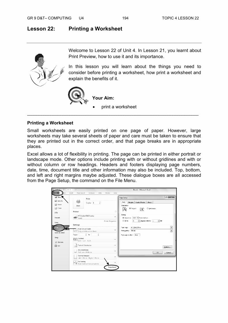
GR 9 D&T– COMPUTING U4 194 TOPIC 4 LESSON 22
Lesson 22: Printing a Worksheet
Welcome to Lesson 22 of Unit 4. In Lesson 21, you learnt about Print Preview, how to use it and its importance.
In this lesson you will learn about the things you need to consider before printing a worksheet, how print a worksheet and explain the benefits of it.
Your Aim:
_________________________________________________________________________
Printing a Worksheet Small worksheets are easily printed on one page of paper. However, large worksheets may take several sheets of paper and care must be taken to ensure that they are printed out in the correct order, and that page breaks are in appropriate places. Excel allows a lot of flexibility in printing. The page can be printed in either portrait or landscape mode. Other options include printing with or without gridlines and with or without column or row headings. Headers and footers displaying page numbers, date, time, document title and other information may also be included. Top, bottom, and left and right margins maybe adjusted. These dialogue boxes are all accessed from the Page Setup, the command on the File Menu.
print a worksheet
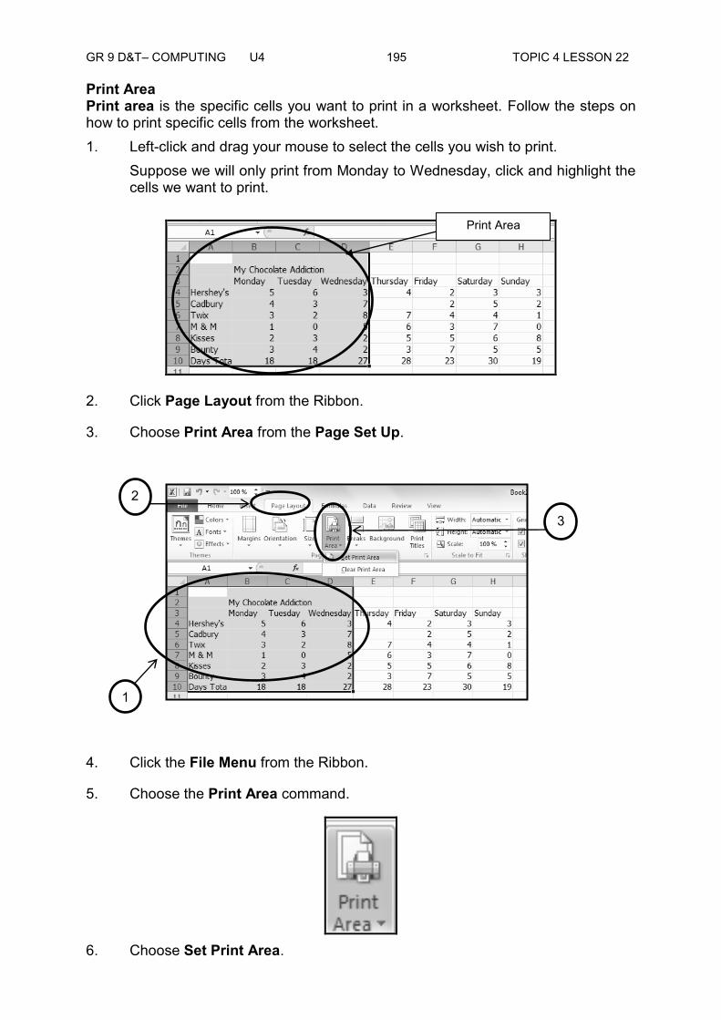
GR 9 D&T– COMPUTING U4 195 TOPIC 4 LESSON 22
Print Area Print area is the specific cells you want to print in a worksheet. Follow the steps on how to print specific cells from the worksheet. 1. Left-click and drag your mouse to select the cells you wish to print.
Suppose we will only print from Monday to Wednesday, click and highlight the cells we want to print.
2. Click Page Layout from the Ribbon.
3. Choose Print Area from the Page Set Up.
4. Click the File Menu from the Ribbon.
5. Choose the Print Area command.
6. Choose Set Print Area.
2
1
3
Print Area
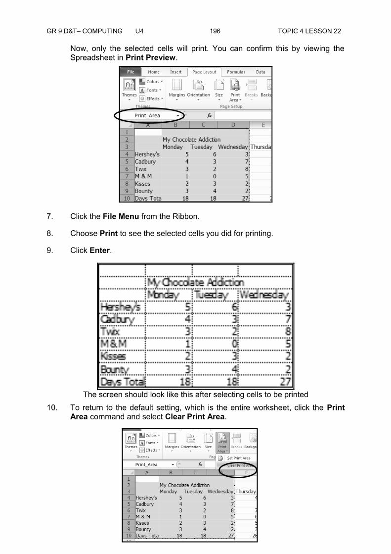
GR 9 D&T– COMPUTING U4 196 TOPIC 4 LESSON 22
Now, only the selected cells will print. You can confirm this by viewing the Spreadsheet in Print Preview.
7. Click the File Menu from the Ribbon.
8. Choose Print to see the selected cells you did for printing.
9. Click Enter.
The screen should look like this after selecting cells to be printed
10. To return to the default setting, which is the entire worksheet, click the Print Area command and select Clear Print Area.

GR 9 D&T– COMPUTING U4 197 TOPIC 4 LESSON 22
To Insert a Break This is to specify where a new page will begin in the printed copy. Page breaks are inserted above and to the left of the selection. Follow the steps on how to insert a break. 1. Click Page Layout from the Ribbon.
2. Select the Breaks command.
3. Click the drop down arrow to select.
4. Click Insert Page Break.
The screen should look like this after selecting Insert Page Break
This is to show where to begin your printing for the first page of your worksheet. And since we only have one page, adjust the horizontal and vertical lines according to the size of our given data.
5. Click the Page Break Preview, you can find it at the bottom right corner of
your screen.

GR 9 D&T– COMPUTING U4 198 TOPIC 4 LESSON 22
After clicking the Page break preview.
6. Click OK to confirm.
The screen will look like this after clicking OK from the Page break preview.
7. As you notice it was divided into two pages. It means that when we print it, it will be printed into two pages. Adjust the page break into one, by positioning the mouse to the horizontal line, the Up-down arrow will appear click it downward.

GR 9 D&T– COMPUTING U4 199 TOPIC 4 LESSON 22
The screen will look like this after has been changed into one page. The Print Titles Command This is an important command to be familiar with if you intend to print your worksheets. It allows you to select specific rows and/or columns to appear on each printed sheet. Imagine how difficult it would be to read Page 48 of a printed Spreadsheet if the column and row headings only appeared on the first page. Follow the steps on how to use the Print Titles command. Follow the steps below on how to print titles.
1. Select the Page Layout tab.
2. Click the Print Titles command. The Page Setup dialog box appears.

GR 9 D&T– COMPUTING U4 200 TOPIC 4 LESSON 22
3. Click the icon at the end of the field.
4. Select rows 2 and 3 in the Spreadsheet that you want to appear on each
printed page.
5. By left clicking rows 2 and 3 to select, you indicate that you want these rows to appear at the top of each page. Repeat for the column, if necessary.
6. Click Enter and OK.
Page Setup Dialogue Box
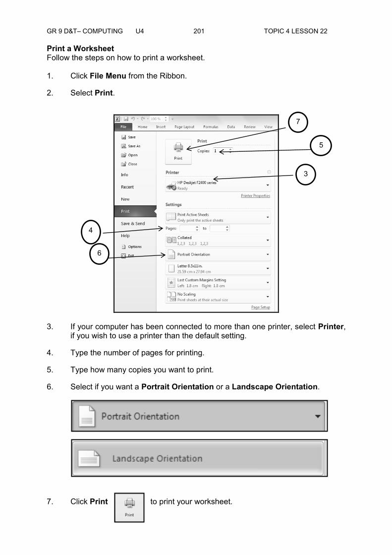
GR 9 D&T– COMPUTING U4 201 TOPIC 4 LESSON 22
Print a Worksheet Follow the steps on how to print a worksheet. 1. Click File Menu from the Ribbon.
2. Select Print.
3. If your computer has been connected to more than one printer, select Printer,
if you wish to use a printer than the default setting.
4. Type the number of pages for printing.
5. Type how many copies you want to print.
6. Select if you want a Portrait Orientation or a Landscape Orientation.
7. Click Print to print your worksheet.
7
3
4
6
5
GR 9 D&T– COMPUTING U4 202 TOPIC 4 LESSON 22
Activity 1: Answer the following.
A. Write the seven steps on how to print a worksheet.
1.
______________________________________________________________
______________________________________________________________
2.
______________________________________________________________
______________________________________________________________
3.
______________________________________________________________
______________________________________________________________
4.
______________________________________________________________
______________________________________________________________
5.
______________________________________________________________
______________________________________________________________
6.
______________________________________________________________
______________________________________________________________
7.
______________________________________________________________
______________________________________________________________
B. Explain the following words. a. Print area
______________________________________________________________
______________________________________________________________
b. Insert break ______________________________________________________________
______________________________________________________________

GR 9 D&T– COMPUTING U4 203 TOPIC 4 LESSON 22
c. Print titles
______________________________________________________________
______________________________________________________________
Thank you for completing this activity. Now, you may go to the end of this lesson to check your answers. Make sure you do the necessary corrections before moving on to the next part of this lesson.
Summary
You have come to the end of Lesson 22. In this lesson you learnt on how to use the print area, to insert a break, to use print titles and to print a worksheet.
NOW DO PRACTICAL EXERCISE 22 ON THE NEXT PAGE

GR 9 D & T– COMPUTING UNIT 4 204 TOPIC 4 LESSON 22
Practice Exercise: 22
___________________________________________________________________
A. Follow the instructions. 1. Let us use the filename Subtraction1 for Printing. Open the file with the
filename Subtraction1. If you lost the file, type the data below in a blank Spreadsheet.
2. Make sure your worksheet has gridlines before printing. 3. Print only cell references A2 to D10. 4. Print only cell references A2 to E7. 5. Print cell references A2 to E7 and A8 to E10. Use the Print Titles command.
Answers to Activity A.
1. Click File Menu from the Ribbon.
2. Select Print.
3. If your computer has been connected to more than one printer, select Printer, if you wish to use a printer than the default setting.
4. Type the number of pages for printing.
5. Type how many copies you want to print.
6. Select if you want a Portrait Orientation or a Landscape Orientation.
7. Click Print to print your worksheet.
B. a. Print Area
Print Area is the specific cells you want to print in a worksheet. b. Insert a Break.
CHECK YOUR WORK. ANSWERS ARE AT THE END OF TOPIC 4.

GR 9 D&T– COMPUTING U4 205 TOPIC 4 LESSON 22
This is to specify where a new page will begin in the printed copy. Page breaks are inserted above and to the left of the selection.
c. Print Titles
This is an important command to be familiar with if you intend to print your worksheets. It allows you to select specific rows and/or columns to appear on each printed sheet.

GR 9 D&T– COMPUTING U4 206 TOPIC 4 LESSON 23
Lesson 23: Creating a Graph with Chart Wizard
Welcome to Lesson 23 of Unit 4. In Lesson 22 you learnt how to open an excel worksheet from a given location and print a worksheet.
In this lesson you will learn the meaning, purpose and importance of creating graph with the Chart Wizard. You will also learn to identify and select appropriate chart for a given data and create graph using Chart Wizard.
Your Aims:
_________________________________________________________________________
Chart Wizard The Chart Wizard feature allows you to build a chart from cells selected within your worksheet.
Charts can be embedded into your current worksheet or added as new worksheets to your workbook file. Chart worksheets are displayed full screen and when printed do not include any worksheet data.
Creating Charts Once a table has been set up, the information in the table can easily be turned into one of several different chart types. These include column and bar graphs, line graphs and pie charts. We can find these charts in Insert tab of the Ribbon
The Charts
define chart wizard and identify its functions and input
identify the location of the Chart Wizard
explore the Chart Wizard
identify the steps on how to use the Chart Wizard
use the Chart Wizard
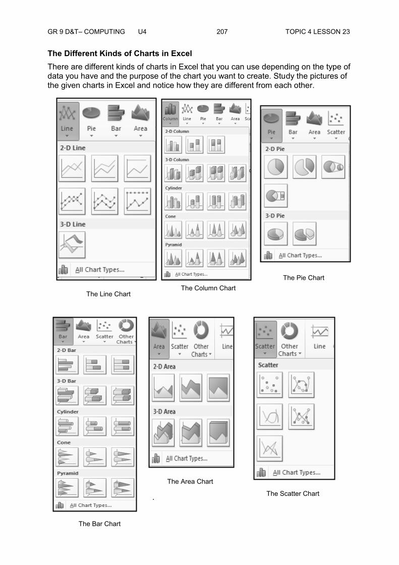
GR 9 D&T– COMPUTING U4 207 TOPIC 4 LESSON 23
The Different Kinds of Charts in Excel There are different kinds of charts in Excel that you can use depending on the type of data you have and the purpose of the chart you want to create. Study the pictures of the given charts in Excel and notice how they are different from each other.
.
The Column Chart
The Line Chart
The Pie Chart
The Bar Chart
The Area Chart
The Scatter Chart

GR 9 D&T– COMPUTING U4 208 TOPIC 4 LESSON 23
Creating a Chart in Excel Follow the steps on how to create a chart in Excel.
1. Select the data to be included in the chart.
2. The selection should include table headings. Excel can use headings as labels on the chart.
3. The selection generally should not include totals.
4. Begin the chart wizard which will prompt you for details about the chart.
5. Customize the completed chart.
Create a Column Chart Let us recall again our data from Lesson 13 which is the Addition1. Follow the steps on how to create a column chart. 1. Select cells A3 to H9. You must select all the cells containing the data you
want in your chart. You should also include the data labels. 2. Choose the Insert tab. 3. Click the Column button in the Charts group. A list of column chart sub-types
types appears.
And Other Charts

GR 9 D&T– COMPUTING U4 209 TOPIC 4 LESSON 23
4. Click the Clustered Column chart sub-type. Excel creates a Clustered Column chart and the Chart Tools context tabs appear.
The screen will look like this after clicking the Clustered Column chart sub-type.
Apply a Chart Layout The Chart Layout changes the overall layout of the chart. Follow the steps on how to apply a chart layout.
1
2
3

GR 9 D&T– COMPUTING U4 210 TOPIC 4 LESSON 23
1. Click your chart. The Chart Tools become available.
2. Choose the Design tab.
3. Click the Quick Layout drop down arrow in the Chart Layouts group. A list of chart layouts appears.
4. Click Layout 5. Excel applies the layout to your chart.

GR 9 D&T– COMPUTING U4 211 TOPIC 4 LESSON 23
The screen will look like this after the Chart Layout was changed to Layout 5.
Add labels Adding labels determine the specific information about the data in your chart. Follow the steps below on how to add labels to your chart.
1. Select Chart Title. Click on Chart Title and then place your cursor before the C in Chart and hold down the Shift key while you use the right arrow key to highlight the words Chart Title.
1

GR 9 D&T– COMPUTING U4 212 TOPIC 4 LESSON 23
2. Type My Chocolate Addiction. Excel adds your title.
3. Select Axis Title and click it. Place your cursor before the A in Axis. Hold down the Shift key while you use the right arrow key to highlight the words Axis Title.
4. Type Days. Excel labels the axis.
After changing the Axis Title.
5. Click anywhere on the chart to end your entry.
Change the Style of a Chart This command changes the overall style of the chart. Follow the steps on how to change the style of a chart.
1. Click your chart. The Chart Tools become available.
2. Choose the Design tab.
3. Click the drop down arrow for more designs in the Chart Styles group. The chart styles appear.
2
3
4

GR 9 D&T– COMPUTING U4 213 TOPIC 4 LESSON 23
4. Click Style 41. Excel applies the style to your chart. Repeat the process to master it.
After selecting Style 41.
1
2
3

GR 9 D&T– COMPUTING U4 214 TOPIC 4 LESSON 23
Change the Size and Position of a Chart The following steps will guide you on how to change the size and position of a chart.
1. Use the handles to adjust the size of your chart. Handles are located in different sides of the chart. Refer to the illustration below for the location of the handles.
2. Click an unused portion of the chart and drag to position the chart beside the data.
1 1
1
1
1
1
1
1
2
GR 9 D&T– COMPUTING U4 215 TOPIC 4 LESSON 23
Activity 1: Answer the following.
1. Give the six different types of a chart.
1. __________________
2. __________________
3. __________________
4. __________________
5. __________________
6. ___________________
B. State the five steps on how to create a chart. 1.
______________________________________________________________
______________________________________________________________
2.
______________________________________________________________
______________________________________________________________
3.
______________________________________________________________
______________________________________________________________
4.
______________________________________________________________
______________________________________________________________
5.
______________________________________________________________
______________________________________________________________
Thank you for completing this activity. Now, you may go to the end of this lesson to check your answer. Make sure you do the necessary corrections before moving on to the next part of this lesson.

GR 9 D&T– COMPUTING U4 216 TOPIC 4 LESSON 23
Summary
You have come to the end of Lesson 23. In this lesson you learnt how to create different graph using the Chart Wizard.
NOW DO PRACTICE EXERCISE 23 ON THE NEXT PAGE.

GR 9 D&T– COMPUTING U4 217 TOPIC 4 LESSON 23
Practice Exercise: 23
A. Perform the following.
1. Open the file with the filename Subtraction1.Let us now apply Graph for our filename Subtraction1.
2. Use the Bar Chart.
3. Select 100% Stacked Bar.
4. Select No. 2 from the Chart Layouts
5. Apply the Chart Title by typing Attendance Tally for Today.
Answers to Activity
A.
1. The Column Chart
2. The Line Chart
3. The Pie Chart
4. The Bar Chart
5. The Area Chart
6. The Scatter Chart
B.
1. Select the data to be included in the chart.
2. The selection should include table headings. Excel can use headings as labels on the chart.
3. The selection generally should not include totals.
4. Begin the chart wizard which will prompt you for details about the chart.
5. Customize the completed chart.
CHECK YOUR WORK. ANSWERS ARE AT THE END OF TOPIC 4.

GR 9 D&T– COMPUTING U4 218 TOPIC 4 LESSON 24
Lesson 24: Incorporating Excel Graphs in Word Processing
Welcome to Lesson 24 of Unit 4. In Lesson 23, you learnt about the meaning and the function of chart wizard. You identified and explored its location and learnt how to use it.
In this lesson, you will identify the process of incorporating Excel graphs in Word document.
Your Aims:
Copy Excel charts to Word Processing Sometimes, it is a lot easier to create your initial tables and charts in Microsoft Excel, and then insert the results into your Microsoft Word document. We will walk through on how to perform such a data import in this step-by-step guide.
Even though Microsoft Word 2010 has a number of outstanding features for table creation, it will never be a match for Excel when it comes to handling data. As such, it’s often a good idea to input your data and create your table or chart in Excel, and then import that information into your Word document.
Steps on how to Insert Excel Data into Word Follow the steps below on how to insert Excel data into Word.
1. Open the Excel Spreadsheet that contains your data, or create a new Spreadsheet and enter your information. In this example, we will use the same filename Subtration1.
Identify the process of incorporating Excel graphs in Word Processing
Add graphs in a word document

GR 9 D&T– COMPUTING U4 219 TOPIC 4 LESSON 24
2. Select all of the cells in your Excel Spreadsheet that you want to insert into
your Word document, and press Ctrl + C on your keyboard to copy the entire selection or click Copy from the Clipboard .
3. Open a blank MS Word document.
4. Place the cursor at the point in the document where you want to insert the data.
5. Open the Home tab on the Word ribbon, and click on the drop down arrow underneath Paste. Select the Paste Special option.
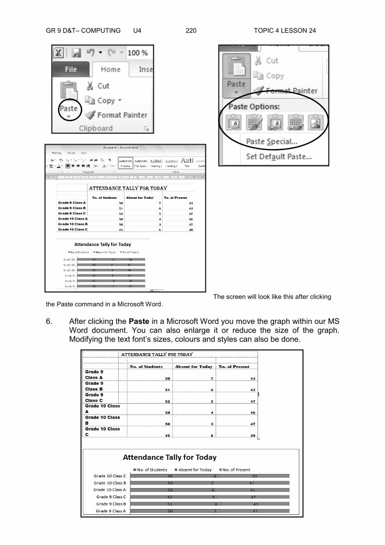
GR 9 D&T– COMPUTING U4 220 TOPIC 4 LESSON 24
The screen will look like this after clicking the Paste command in a Microsoft Word. 6. After clicking the Paste in a Microsoft Word you move the graph within our MS
Word document. You can also enlarge it or reduce the size of the graph. Modifying the text font’s sizes, colours and styles can also be done.

GR 9 D&T– COMPUTING U4 221 TOPIC 4 LESSON 24
Activity 1: Follow the instructions.
A. Give the short cut keys of the keyboard for the following commands.
1. Paste ___________________
2. Cut _____________________
3. Copy _____________________
B. Give three steps on how to Copy / Paste a graph from an Excel to Word Processing.
1.
______________________________________________________________
______________________________________________________________
2.
______________________________________________________________
______________________________________________________________
3.
______________________________________________________________
______________________________________________________________
______________________________________________________________
Thank you for completing this activity. Now, you may go to the end of this lesson to check your answer. Make sure you do the necessary corrections before moving on to the next part of this lesson.
Summary
You have come to the end of Lesson 24. In this lesson you learnt on how to incorporate the Excel graph in Word processing.
NOW DO PRACTICE EXERCISE 24 ON THE NEXT PAGE.
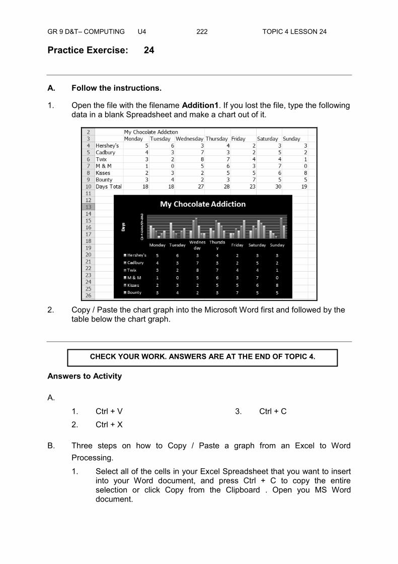
GR 9 D&T– COMPUTING U4 222 TOPIC 4 LESSON 24
Practice Exercise: 24
A. Follow the instructions.
1. Open the file with the filename Addition1. If you lost the file, type the following data in a blank Spreadsheet and make a chart out of it.
2. Copy / Paste the chart graph into the Microsoft Word first and followed by the
table below the chart graph.
Answers to Activity
A. 1. Ctrl + V 2. Ctrl + X
3. Ctrl + C
B. Three steps on how to Copy / Paste a graph from an Excel to Word Processing.
1. Select all of the cells in your Excel Spreadsheet that you want to insert into your Word document, and press Ctrl + C to copy the entire selection or click Copy from the Clipboard . Open you MS Word document.
CHECK YOUR WORK. ANSWERS ARE AT THE END OF TOPIC 4.

GR 9 D&T– COMPUTING U4 223 TOPIC 4 LESSON 24
2. Place the cursor at the point in the document where you want to insert
the data. 3. Open the Home tab on the Word ribbon, and click on the drop down
arrow underneath Paste.

GR 9 D&T– COMPUTING U4 224 TOPIC 4 ANSWERS
Answers to Practice Exercises Topic 4
___________________________________________________________________
Practice Exercise 19 a.
b.

GR 9 D&T– COMPUTING U4 225 TOPIC 4 ANSWERS
c.
d.

GR 9 D&T– COMPUTING U4 226 TOPIC 4 ANSWERS
e.

GR 9 D&T– COMPUTING U4 227 TOPIC 4 ANSWERS
Practice Exercise 20
Practice Exercise 21
1.
2.
With gridlines
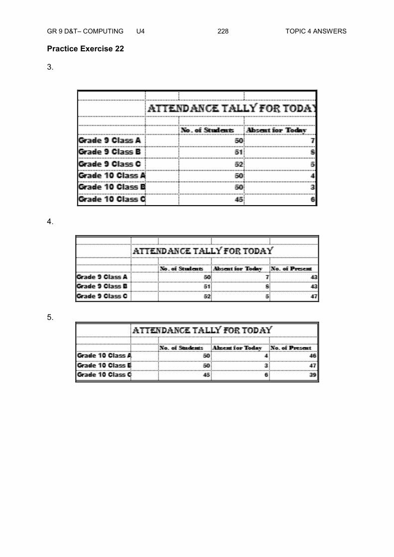
GR 9 D&T– COMPUTING U4 228 TOPIC 4 ANSWERS
Practice Exercise 22 3.
4.
5.

GR 9 D&T– COMPUTING U4 229 TOPIC 4 ANSWERS
Practice Exercise 23
Practice Exercise 24
___________________________________________________________________
End of Topic 4
Now Do Exercise 4 in Assignment Book 4.

GR 9 D&T– COMPUTING U4 230 GLOSSARY
3-D reference A reference to a range that spans two or more worksheets in a workbook. 3-D walls and floor The areas surrounding many 3-D chart types that give dimension and boundaries to the chart. Two walls and one floor are displayed within the plot area. Activate To make a chart sheet or worksheet the active, or selected, sheet. The sheet that you activate determines which tabs are displayed. To activate a sheet, click the tab for the sheet in the workbook. Active Cell. Is an intersection of a column and row. It receives the data or the command given to it. Active Sheet The sheet that you're working on in a workbook. The name on the tab of the active sheet is bold. Address The path to an object, document, file, page, or other destination. An address can be a URL (Web address) or a UNC path (network address), and can include a specific location within a file, such as a Word bookmark or an Excel cell range. Argument The values that a function uses to perform operations or calculations. The type of argument a function uses is specific to the function. Common arguments that are used within functions include numbers, text, cell references, and names. Array Used to build single formulas that produce multiple results or that operate on a group of arguments that are arranged in rows and columns. An array range shares a common formula; an array constant is a group of constants used as an argument. Attribute. See also field.
Axis A line bordering the chart plot area used as a frame of reference for measurement. The y axis is usually the vertical axis and contains data. The x-axis is usually the horizontal axis and contains categories. Base Address The relative path that Excel uses for the destination address when you insert a hyperlink. This can be an Internet address (URL), a path to a folder on your hard drive, or a path to a folder on a network. Border A decorative line that can be applied to worksheet cells or objects, such as charts, pictures, or text boxes. Borders distinguish, emphasize, or group items. Chart. Is a graphic representation of data. It allows the user to see what the results of data to better understand and predict current and future data. Cell. Is the intersection between a row and a column on a spreadsheet that starts with cell A1. Cell Address. See also Active Cell.

GR 9 D&T– COMPUTING U4 231 GLOSSARY
Cell Attributes. Allows a user to define the appearance of spreadsheet. Cell Reference. Is the particular cell (or range) for which the attribute value need to be returned. Close. A command that is used to close a Spreadsheet. Columns. Referred by alphabetic characters in the grey boxes that run across the Excel screen. Column Field A field that's assigned a column orientation in a PivotTable report. Items associated with a column field are displayed as column labels. Column Heading The shaded area at the top of each Data pane column that contains the field name. Comments. Hidden text that enables users to make comments about cells and their values. Complex Formulas. Involve more than one mathematical operation. It allows the user to manipulate more numbers for data interpretation. It provides the user flexibility to manipulate operations as needed in any data evaluation. Constant A value that is not calculated. For example, the number 210 and the text "Quarterly Earnings" are constants. An expression, or a value resulting from an expression, is not a constant. Constraints The limitations placed on a Solver problem. You can apply constraints to adjustable cells, the target cell, or other cells that are directly or indirectly related to the target cell. Copy Area The cells that you copy when you want to paste data into another location. After you copy cells, a moving border appears around them to indicate that they've been copied. Data Form A dialog box that displays one complete record at a time. You can use data forms to add, change, locate, and delete records. Data Label A label that provides additional information about a data marker, which represents a single data point or value that originates from a datasheet cell. Data Marker A bar, area, dot, slice, or other symbol in a chart that represents a single data point or value that originates from a datasheet cell. Related data markers in a chart constitute a data series. Data Pane The area of the window that displays the result set of your query.

GR 9 D&T– COMPUTING U4 232 GLOSSARY
Data Points Individual values that are plotted in a chart. Related data points make up a data series. Data points are represented by bars, columns, lines, slices, dots, and other shapes. These shapes are called data markers. Data Region A range of cells that contains data and that is bounded by empty cells or datasheet borders. Data Series Related data points that are plotted in a chart and originate from datasheet rows or columns. Each data series in a chart has a unique colour or pattern. You can plot one or more data series in a chart. Pie charts have only one data series. Data Source A stored set of "source" information used to connect to a database. A data source can include the name and location of the database server, the name of the database driver, and information that the database needs when you log on. Data Source Driver A program file used to connect to a specific database. Each database program or management system requires a different driver. Data Table A range of cells that shows the results of substituting different values in one or more formulas. There are two types of data tables: one-input tables and two-input tables. Database A collection of data related to a particular subject or purpose. Within a database, information about a particular entity, such as an employee or order, is categorized into tables, records, and fields. Default Workbook Template The Book.xlt template that you create to change the default format of new workbooks. Excel uses the template to create a blank workbook when you start Excel or create a new workbook without specifying a template. Default Worksheet Template The Sheet.xlt template that you create to change the default format of new worksheets. Excel uses the template to create a blank worksheet when you add a new worksheet to a workbook. Dependents Cells that contain formulas that refer to other cells. For example, if cell D10 contains the formula =B5, cell D10 is a dependent of cell B5. Destination Area The range of cells that you select to hold the summarized data in a consolidation. The destination area can be on the same worksheet as the source data or on a different worksheet. A worksheet can contain only one consolidation. Detail Data For automatic subtotals and worksheet outlines, the subtotal rows or columns that are totaled by summary data. Detail data is typically adjacent to and either above or to the left of the summary data.

GR 9 D&T– COMPUTING U4 233 GLOSSARY
Drop Lines In line and area charts, lines that extend from a data point to the category (x) axis. Useful in area charts to clarify where one data marker ends and the next begins. Drop-Down List Box A control on a menu, toolbar, or dialog box that displays a list of options when you click the small arrow next to the list box. Embedded Chart A chart that is placed on a worksheet rather than on a separate chart sheet. Embedded charts are beneficial when you want to view or print a chart or a PivotChart report with its source data or other information in a worksheet. Error Bars Usually used in statistical or scientific data, error bars show potential error or degree of uncertainty relative to each data marker in a series. Excel add-in Components that can be installed on your computer to add commands and functions to Excel. These add-in programs are specific to Excel. Other add-in programs that are available for Excel or Office are Component Object Model (COM) add-ins. Excel table Formerly known as an Excel list, you can create, format, and expand an Excel table to organise the data on your worksheet. Expression A combination of operators, field names, functions, literals, and constants that evaluates to a single value. Expressions can specify criteria (such as Order Amount>10000) or perform calculations on field values (such as Price*Quantity). External Data Data that is stored in a database, such as Access, dBASE, or SQL Server, that is separate from Query and the program from which you started Query. Field. Is a single item of data within a database or software program. Font. Commands let you change the style, size, and colour of text. Formatting Attributes. Cells can contain formatting attributes that change the way letters, numbers, and dates are displayed. Formula. Is an expression telling the computer what mathematical operation to perform upon a specific value. It allows quick calculations and get totals of multiple cells, rows, or columns in spreadsheet. Formula Bar. Displays information entered or being entered as you type-in the current or active cell. The contents of a cell can also be edited in the Formula Bar. Functions. Are designed to provide one word access to a series of operations. Grid A set of intersecting lines used to align objects. Gridlines in Charts Lines you can add to a chart that make it easier to view and evaluate data. Gridlines extend from the tick marks on an axis across the plot area. Group In an outline or PivotTable report, one or more detail rows or columns that are adjacent and subordinate to a summary row or column.

GR 9 D&T– COMPUTING U4 234 GLOSSARY
High-Low Lines In 2-D line charts, lines that extend from the highest to the lowest value in each category. High-low lines are often used in stock charts. History worksheet A separate worksheet that lists changes being tracked in a shared workbook, including the name of the person who made the change, when and where it was made, what data was deleted or replaced, and how conflicts were resolved. Horizontal Scroll Bar. Located at the bottom of the screen is used to move left or right across the spreadsheet. Identifier A field name used in an expression. For example, Order Amount is the identifier (field name) for a field that contains order amounts. You can use an expression (such as Price*Quantity) in place of an identifier. Index A database component that speeds up searching for data. When a table has an index, data in the table can be found by looking it up in the index. Input Cell The cell in which each input value from a data table is substituted. Any cell on a worksheet can be the input cell. Although the input cell does not need to be part of the data table, the formulas in data tables must refer to the input cell. Insert Row In an Excel table, a special row that facilitates data entry. The Insert row is indicated by an asterisk. Landscape. Is the orientation of the page that prints the image horizontally across the page instead of vertically. Mapped Range A range in an XML list that has been linked to an element in an XML map. Matrix A rectangular array of values or a range of cells that is combined with other arrays or ranges to produce multiple sums or products. Excel has predefined matrix functions that can produce the sums or products. Merged Cell A single cell that is created by combining two or more selected cells. The cell reference for a merged cell is the upper-left cell in the original selected range. Microsoft Excel control A native Excel control other than an ActiveX control. Name A word or string of characters that represents a cell, range of cells, formula, or constant value. Use easy-to-understand names, such as Products, to refer to hard to understand ranges, such as Sales!C20:C30. Name Box. Displays the cell reference of the active cell. It will also show the name assigned to a cell or range of cells. The Name Box can also be used to assign names to cells or range of cells. New. Command tat is used to create a new Workbook.

GR 9 D&T– COMPUTING U4 235 GLOSSARY
Open. A command that is used to open n existing file from a flash drive or hard drive of your computer. Operand Items on either side of an operator in a formula. In Excel, operands can be values, cell references, names, labels, and functions. Operator A sign or symbol that specifies the type of calculation to perform within an expression. There are mathematical, comparison, logical, and reference operators. Outline Worksheet data in which rows or columns of detail data are grouped so that you can create summary reports. The outline can summarize either an entire worksheet or a selected portion of it. Outline Data The data that is contained within a worksheet outline. Outline data includes both the summary and detail rows or columns of an outline. Outline Symbols Symbols that you use to change the view of an outlined worksheet. You can show or hide detailed data by pressing the plus sign, minus sign, and the numbers 1, 2, 3, or 4, indicating the outline level. Page Break Divider that breaks a worksheet into separate pages for printing. Excel inserts automatic page breaks based on the paper size, margin settings, scaling options, and the positions of any manual page breaks that you insert. Page Break Preview Worksheet view that displays the areas to be printed and the locations of page breaks. The area to be printed is displayed in white, automatic page breaks appear as dashed lines, and manual page breaks appear as solid lines. Parameter In Excel, you can add, change, or remove parameters to specify cells that are editable in the viewable worksheet data of Excel Services. When you save the workbook, the changes are automatically reflected on the server. Password A way to protect your worksheet or workbook. When you protect worksheet or workbook elements with a password, it is very important that you remember that password. Without it, there is no way to unprotect the workbook or worksheet. You should always use strong passwords that combine uppercase and lowercase letters, numbers, and symbols. Weak passwords don't mix these elements. Strong password: Y6dh!et5. Weak password: House27. Use a strong password that you can remember so that you don't have to write it down. Paste Area The target destination for data that's been cut or copied by using the Office Clipboard. Primary Key One or more fields that uniquely identify each record in a table. In the same way that a license plate number identifies a car, the primary key uniquely identifies a record.
GR 9 D&T– COMPUTING U4 236 GLOSSARY
Print Area One or more ranges of cells that you designate to print when you don't want to print the entire worksheet. If a worksheet includes a print area, only the print area is printed. Portrait Orientation. Is the orientation of the page that prints the image vertically across the page instead of horizontally. Quantitative Data. Data that can be represented in the form of a number. This data can be used for statistical analysis and gives greater accuracy in the final result. Qualitative Data. Data that cannot be represented in the form of a number but rather expressed as other variables like meanings of ambiguous words, gender classification, religious preferences. Quick Access Toolbar. Is located above the Ribbon, and it lets you access common commands no matter which tabs you are on. It shows, the Save, Undo, and Repeat commands by default. Range Two or more cells on a sheet. The cells in a range can be adjacent or nonadjacent. Read-only A setting that allows a file to be read or copied but not changed or saved. Record A collection of information about a particular person, place, event, or thing. When Query displays a result set in the Data pane, a record is represented as a row. Ribbon. Contain multiple tabs each with several groups of commands. You can add your own tabs that contain your favourite commands. Rows. Are referred by numbers that appear on the left and then run down the Excel screen. Row Heading The numbered gray area to the left of each row. Click the row heading to select an entire row. To increase or decrease the height of a row, drag the line below the row heading. Row Label A field that's assigned a row orientation in a PivotTable report. Save. A command that is used to save a file that has had changes made to it. Save As. A command that is used to save a new file for the first time or save an existing file with a different name. Sheet Tabs. Separated workbook into specific worksheets. Sorting. Is process of organising data in a particular order allowing for information to be found easier. Spreadsheet. Is the application that launched the personal computer into the business world. A spreadsheet provides way to set up relationships between numbers. Table Pane The area of the Query window that displays the tables in a query. Each table displays the fields from which you can retrieve data.

GR 9 D&T– COMPUTING U4 237 GLOSSARY
Template A workbook that you create and use as the basis for other similar workbooks. You can create templates for workbooks and worksheets. The default template for workbooks is called Book.xlt. The default template for worksheets is called Sheet.xlt. Text. Cells can contain letters, numbers, and dates. Text Box A rectangular object on a worksheet or chart, in which you can type text. Text Attribute. Refers to how a particular font is presented. Total Row A special row in an Excel table that provides a selection of aggregate functions useful for working with numerical data. Totals One of the five calculation types Query defines for you: Sum, Avg, Count, Min, and Max. Vertical Scroll Bar. Located along the right edge of the screen. It is used to move up or down the spreadsheet View A set of display and print settings that you can name and apply to a workbook. You can create more than one view of the same workbook without saving separate copies of the workbook. VisiCalc. Short for Visible Calculator. The first Spreadsheet programme and the first fully functional computer application to run on personal computers. Worksheet. Is organised into a rectangular grid containing columns (vertical) and rows (horizontal).