GPU Techniques: Novel Approaches to Deformation and Fracture within Videogames Morris, D. Submitted version deposited in CURVE January 2014 Original citation: Morris, D. (2010). GPU techniques: novel approaches to deformation and fracture within videogames. Unpublished MResThesis. Coventry: Coventry University. Copyright © and Moral Rights are retained by the author(s) and/ or other copyright owners. A copy can be downloaded for personal non-commercial research or study, without prior permission or charge. This item cannot be reproduced or quoted extensively from without first obtaining permission in writing from the copyright holder(s). The content must not be changed in any way or sold commercially in any format or medium without the formal permission of the copyright holders.

CURVE is the Institutional Repository for Coventry University

http://curve.coventry.ac.uk/open

GPU Techniques: Novel Approaches to

Deformation and Fracture within

Videogames

Derek John Morris

Interactive Worlds Applied Research Group

A thesis submitted in partial fulfilment of the requirements of

Coventry University for the degree of

Master of Science by Research

Submitted: December 2010

This copy of the thesis has been supplied on condition that anyone who consults

it is understood to recognise that its copyright rests with its author and due ac-

knowledgement must always be made of the use of any material contained in, or

derived from, this thesis.

i

GPU Techniques: Novel Approaches to

Deformation and Fracture within Videogames

Derek John Morris

Abstract

An investigation is introduced into methods of utilising current Graphics Pro-

cessing Unit (GPU) features to migrate algorithms that are traditionally imple-

mented on the Central Processing Unit (CPU).

The deformation, fracture and procedural edges sections of a destructible

material simulation are implemented whilst developing novel solutions in order

to improve performance and reduce content creation time.

The implementation takes the form of a simulation prototype and is spe-

cific to DirectX and HLSL, chosen because this target environment has enjoyed

widespread use in the videogame demographic and is readily available on the PC

platform although the implications of the work should be generalisable to systems

running on other platforms or environments. The implementation also does not

make use of General Purpose Graphics Processing Unit (GPGPU) Application

Programming Interfaces (API’s) such as OpenCL [Khronos 2010a] and Direct-

Compute [NVIDIA 2010b], or specialist configurations such as Nvidias PhysX

[NVIDIA 2010c] or CUDA [NVIDIA 2011] that are targeted at hardware from a

specific vendor as this research aims to encompass all compliant graphics hardware

and allow the easiest possible adoption of any developed techniques, leveraging

the large amount of knowledge within the videogame industry of the standard

rendering pipeline and associated API’s.

The outcome demonstrates a destructible material simulation with a CPU and

GPU implementation running on two different PC hardware configurations with

both wood and rubber material types. The Frames Per Second (FPS) are recorded

for comparison and the instability of the explicit Euler numerical integrator used

is highlighted along with suggestions for improvement with future work.

ii

A chapter is also provided covering some of the GPU best practices and tips

for implementation of the GPU algorithms detailed, drawn from the experience

gained whilst performing the required research to build the simulation prototype

(see Chapter 5).

iii

This thesis is dedicated to my brother, David Morris, who always

believes in me, no matter what.

iv

Acknowledgements

A big thanks to my Director of Studies, Dr Eike F Anderson for guiding and

teaching me along the way and to my second supervisor, Dr Chris Peters for his

valuable feedback.

I am grateful to my viva voce examining panel, Dr Kurt Debattista, Professor

Anne James and Dr Rob James for their comments and suggestions that have

allowed me to improve the quality of this final version of the thesis.

Also, many thanks to David, Kerry and Riley for keeping me sane throughout

this whole process.

v

Contents

List of Figures ix

1 Introduction 1

1.1 Aims . . . . . . . . . . . . . . . . . . . . . . . . . . . . . . . . . . 2

1.2 Contribution . . . . . . . . . . . . . . . . . . . . . . . . . . . . . . 4

1.3 Thesis Overview . . . . . . . . . . . . . . . . . . . . . . . . . . . . 5

I Research 7

2 Background 8

2.1 GPU History . . . . . . . . . . . . . . . . . . . . . . . . . . . . . 9

2.2 Deformation . . . . . . . . . . . . . . . . . . . . . . . . . . . . . . 11

2.3 Fracture . . . . . . . . . . . . . . . . . . . . . . . . . . . . . . . . 14

2.4 Numerical Integration . . . . . . . . . . . . . . . . . . . . . . . . 15

II Simulation 17

3 Overview 18

4 Framework 20

5 GPU Techniques Used 22

5.1 Rendering Pipeline . . . . . . . . . . . . . . . . . . . . . . . . . . 22

5.2 Optimisations . . . . . . . . . . . . . . . . . . . . . . . . . . . . . 24

vi

CONTENTS

6 Deformation 27

6.1 Method . . . . . . . . . . . . . . . . . . . . . . . . . . . . . . . . 27

6.2 Implementation . . . . . . . . . . . . . . . . . . . . . . . . . . . . 29

7 Fracture 35

7.1 Method . . . . . . . . . . . . . . . . . . . . . . . . . . . . . . . . 35

7.2 Implementation . . . . . . . . . . . . . . . . . . . . . . . . . . . . 36

8 Procedural Edges 40

8.1 Method . . . . . . . . . . . . . . . . . . . . . . . . . . . . . . . . 40

8.2 Implementation . . . . . . . . . . . . . . . . . . . . . . . . . . . . 41

III Conclusions 44

9 Results and Discussion 45

10 Summary of Contributions 54

11 Future Work 55

Appendices 57

A HLSL Code Listing 58

A.1 eig3.fxh . . . . . . . . . . . . . . . . . . . . . . . . . . . . . . . . 58

A.2 wall.fx . . . . . . . . . . . . . . . . . . . . . . . . . . . . . . . . . 64

References 74

vii

List of Figures

2.1 Graphics rendering pipeline. . . . . . . . . . . . . . . . . . . . . . 9

5.1 DirectX 10 rendering pipeline. . . . . . . . . . . . . . . . . . . . . 23

6.1 Tetrahedron and its nodes. . . . . . . . . . . . . . . . . . . . . . . 27

6.2 Cube composed of five tetrahedra. . . . . . . . . . . . . . . . . . . 28

6.3 Wall composed of tetrahedron cubes. . . . . . . . . . . . . . . . . 28

6.4 Finite element update method (initial version). . . . . . . . . . . . 32

6.5 Node update method. . . . . . . . . . . . . . . . . . . . . . . . . . 33

6.6 Simulation draw method. . . . . . . . . . . . . . . . . . . . . . . . 34

7.1 New finite element connectivity. . . . . . . . . . . . . . . . . . . . 36

7.2 Finite element update method (extended version). . . . . . . . . . 37

7.3 Fracture update method. . . . . . . . . . . . . . . . . . . . . . . . 38

7.4 Connectivity update method. . . . . . . . . . . . . . . . . . . . . 39

8.1 Display draw method. . . . . . . . . . . . . . . . . . . . . . . . . 43

9.1 Deformation on rubber material. . . . . . . . . . . . . . . . . . . . 49

9.2 Deformation wireframe. . . . . . . . . . . . . . . . . . . . . . . . . 49

9.3 Fracture on wood material (i). . . . . . . . . . . . . . . . . . . . . 50

9.4 Fracture on wood material (ii). . . . . . . . . . . . . . . . . . . . 50

9.5 Fracture wireframe. . . . . . . . . . . . . . . . . . . . . . . . . . . 51

9.6 Procedural edges on wood material (i). . . . . . . . . . . . . . . . 51

9.7 Procedural edges on wood material (ii). . . . . . . . . . . . . . . . 52

9.8 Procedural edges wireframe. . . . . . . . . . . . . . . . . . . . . . 52

viii

LIST OF FIGURES

9.9 Simulation stress test. . . . . . . . . . . . . . . . . . . . . . . . . 53

ix

Chapter 1

Introduction

In recent years, videogames have become increasingly complex, aiming to immerse

the player in virtual game worlds that employ 3D animated graphics to provide

players with the illusion of realism. A major contributing factor to this end

has been a steep rise in the quality of real-time computer graphics, fuelled by

dramatic advances in computer graphics hardware combined with the evolution

of algorithms and methods that more realistically model the real world.

One particular area that contributes significantly to the perception of a realis-

tic virtual environment is the behaviour of materials when they are broken apart

or destroyed. Examples of these deformable and destructible materials within

the setting of a videogame could be the shattering of a glass window pane as it

is riddled with gunfire or the crumbling of a brick wall as it is smashed with a

wrecking ball.

There have been many advances gained from the research into this field over

the last two decades that together with the ever increasing computational power

available, has allowed this area of computer graphics to move from the offline into

the real-time domain and therefore become a prevalent feature within videogames.

Traditionally, this research has been based around CPU implementations. This

is partially due to the lack of dedicated graphics hardware in the early days

and also the fact that the required physics based algorithms require memory

scatter and gather techniques [Gummaraju and Rosenblum 2005] that are much

more straight-forward to implement on a CPU due to the nature of the hardware

design.

1

1.1 Aims

As GPU technology has evolved over the years, traditionally fixed aspects of

the hardware accelerated graphics pipeline have become programmable allowing

more flexibility with the types of algorithms that can be implemented. With

the advent of technologies such as vertex shaders, pixel shaders, multiple render

targets (MRT’s) and more recently, geometry shaders and a stream out mecha-

nism [MSDN 2010d], it has become possible to treat the GPU more as a general

purpose data stream processor, therefore allowing for the possibility of migrating

previously CPU based algorithms onto the GPU. Significant research has been

carried out developing high level languages and constructs that serve to aid with

this transition [Buck et al. 2004].

In the arena of videogames, it can be very beneficial to have algorithms imple-

mented on the GPU for two key reasons: for those that require the same process

to be carried out on many different data elements and the data elements are not

dependant on each other, then the parallel architecture of the GPU can process

the data asynchronously and greatly increase performance [Buck et al. 2004]. The

other key reason is that an algorithm can be implemented on both the CPU and

GPU allowing for effective load balancing of the overall system by distributing

the work load across the two processors.

Drawing on over a decade of personal experience within the videogame in-

dustry and discussing with colleagues the issue of improving algorithm and code

performance, it was felt that it would be advantageous to this area of research

to develop some GPU based techniques that take previously CPU based algo-

rithms and migrate them across to run on the GPU utilising the latest hardware

features. As a case study, sections of a deformation and fracture simulation will

be implemented on the GPU whilst also developing novel solutions to improve

performance and reduce content creation time. Also, it would be of maximum

benefit if the algorithms were to run on a wide range of graphics hardware so as

to be applicable to the largest number of potential users.

1.1 Aims

The work aims to investigate the methods and techniques of utilising current GPU

features to migrate algorithms that are traditionally implemented on the CPU.

2

1.1 Aims

The deformation, fracture and procedural edges sections of a destructible material

simulation are implemented whilst developing novel solutions in order to improve

performance and reduce content creation time. The outcome is applicable for use

within a videogame or similar real-time graphics application.

A complete simulation of destructible and deformable materials covers many

different areas including deformation, fracture, collisions, advanced numerical in-

tegration methods and a content creation toolchain. For the purposes of keeping

this research scope manageable and focusing on novel GPU techniques, the sim-

ulation areas covered will be deformation and fracture. In each of these areas,

the desired outcome is to produce a design that has the majority of processing

(i.e. the work that takes the most processor cycles to complete) implemented on

the GPU in order to make the most efficient use of system resources. To main-

tain focus on the migration of previous methods from CPU to GPU processing,

the design produces an acceptable perceived visual representation based on the

author’s experience within the videogame industry, that has the possibility for

future refinement rather than attempting to provide the best possible accuracy

and stability.

In addition to the migration of previous methods to the GPU for deformation

and fracture, investigation is made into novel techniques of producing the edges

of destroyed materials. If these edges can be created procedurally and remain

visually pleasing then this would reduce the time required to create the artistic

content necessary to portray a material.

The investigation and design of the system is demonstrated by producing a

prototype simulator that shows the realistic destruction of a sample range of

materials by visually depicting the deformation and fracture when a wall made

up of the simulated material is broken apart.

A basic CPU implementation that consists of a direct implementation of the

used algorithms without optimisations is used for comparison as this provides a

reliable indicator of CPU algorithm capabilities and a baseline to compare the

GPU implementation against. Optimisations are possible to the CPU implemen-

tation, for example running across multiple threads or processors but this can

take a long time to implement, and as the main focus is to move CPU algorithms

onto the GPU, this would detract from the purpose of the research.

3

1.2 Contribution

The implementation takes the form of a simulation prototype and is spe-

cific to DirectX and HLSL, chosen because this target environment has enjoyed

widespread use in the videogame demographic and is readily available on the PC

platform although the implications of the work should be generalisable to systems

running on other platforms or environments. The implementation also does not

make use of GPGPU API’s such as OpenCL[Khronos 2010a] and DirectCompute

[NVIDIA 2010b], or specialist configurations such as Nvidias PhysX [NVIDIA

2010c] or CUDA [NVIDIA 2011] that are targeted at hardware from a specific

vendor as this research aims to encompass all compliant graphics hardware and

allow the easiest possible adoption of any developed techniques.

1.2 Contribution

The specific areas of contribution from this thesis to the field of computer graphics

are:

• Design and implementation details showing an efficient method of migrating

previously CPU implemented algorithms onto the GPU.

• Develop generic GPU best practices with the aim of increasing the perfor-

mance of a videogame or similar real-time graphics application.

• Procedural geometry creation techniques to define the edges of destroyed

materials that allow fractured materials to look visually realistic, and due to

their automated construction, produce a saving in valuable content creation

time.

• Description covering all of the algorithms and techniques required to im-

plement the deformation and fracture sections used within a simulation of

destructible materials with the majority of processing being carried out on

the GPU.

4

1.3 Thesis Overview

1.3 Thesis Overview

This thesis is divided into three parts. Part I gives an overview of the evolution

of GPU technology and reviews the work done to date on destructible material

simulations in the field of computer graphics. Part II describes the design and

implementation of the deformation and fracture sections of a destructible material

simulation implemented on the GPU. Part III discusses the conclusions drawn

from this research project and suggestions for future work.

The aim of the discussion is to highlight the simulation sections of deformation

and fracture and supply detailed information on how to construct such a simu-

lation. Along with the specifics of the GPU implementation, any algorithm or

coding differences between the CPU and GPU implementations are highlighted.

Comparisons are made between the processor time usage of the two alternate

implementations and finally suggestions for future improvements or expansions

are made.

An overview of each chapter is as follows:

Chapter 2 provides information on the evolution of GPU graphics hardware

and the ever increasing feature set available for supporting hardware accelerated

algorithm implementations. The history into the research that has been carried

out over the last two decades with relation to deformable and destructible ma-

terials is also presented. These span from the initial offline elasticity methods

of deformation published in 1987, various fracture methods implemented both

offline and in real-time, through to a fully functioning CPU based middleware

solution that has been integrated into several top selling videogames.

Chapter 3 gives an overview of the simulation created in order to present

this work. The implementation environment is outlined in addition to the design

decisions taken that are specific to the simulation.

Chapter 4 describes the framework and environment used to develop the

simulation prototype.

Chapter 5 details the GPU features used along with best practices for the

best performance usage within a videogame or real-time graphics environment.

Chapter 6 describes the GPU implementation of the physics based de-

formable material methods used within the simulation. Data structures and flow

5

1.3 Thesis Overview

diagrams of the design are provided detailing each stage of the implementation.

The changes required to migrate processing from the CPU to the GPU are high-

lighted along with any idiosyncrasies encountered.

Chapter 7 explains the methods used to form cracks and break apart a ma-

terial (i.e. fracture) when areas in the material exceed a certain stress threshold.

The data structures and flow diagrams from the preceding chapter are expanded

upon and the simulation is extended to both deform and fracture in a physically

realistic manner.

Chapter 8 introduces the procedural generation for the material edges that

have been broken apart. An attempt is made to simulate the visual representa-

tion of these splinters in a manner that is not necessarily physically correct but

provides acceptable visual results with low computational overhead and minimal

developer content creation time.

Chapter 9 evaluates the simulation results by comparing the output depict-

ing the deformation and destruction across a sample range of materials. The

results of the simulation are discussed in relation to the research as a whole.

Also, any concerns or issues raised with the implementation methods used for the

entire simulation are outlined.

Chapter 10 provides a summary of the contributions made to the area of

research and novel techniques described with this thesis.

Chapter 11 discusses possible improvements that could be made to the sim-

ulation along with expansion ideas. Also suggestions are made for areas that

could benefit from future research and development.

6

Part I

Research

7

Chapter 2

Background

The computer graphics rendering pipeline was originally performed on CPU pro-

cessors and over the last two decades dedicated graphics acceleration hardware

has been introduced into the marketplace that not only increases computational

performance, but provides much more flexibility with the processing performed.

The most recent GPU’s are so flexible and capable of performing advanced cal-

culations that it is becoming possible to implement a wide range of algorithms

on the hardware that were previously confined to the CPU only.

Deformation and fracture of materials in the field of computer graphics takes a

heavy influence from the physical models used in engineering disciplines. For real-

time simulations, these physical models are then simplified as much as possible to

maintain a favourable balance between performance and accuracy. In the area of

real-time computer graphics, it is usually acceptable to reduce physical accuracy

as long as the perceived visual representation remains plausible.

The leading research on deformable models derives from a branch of contin-

uum mechanics called elasticity theory which models the deformation of solid

objects by calculating the internal stresses and strains generated from applied

loads. The simplification of elasticity theory most commonly used in real-time

computer graphics is linear elasticity theory which maintains a linear relationship

between the stresses and strains and is therefore less computationally expensive

than its nonlinear counterpart.

When stresses exceed a certain threshold, materials in the physical world

either stretch out of shape before cracking and breaking apart or immediately

8

2.1 GPU History

crack and break apart based on the properties of the material. Previous research

on fracture concerns itself with the modelling of this stretching effect using the

model of plasticity and also the generation and propagation of the cracks, which

in turn lead to the separation of the material into discrete entities. Fracture in the

area of real-time computer graphics is based on these physical models with the

emphasis being on the visual representation of the effect rather than the physical

accuracy.

In order to apply these physical models to a computer simulation they are nu-

merically integrated across discrete timesteps to build up a convincing represen-

tation of motion over time. The integration schemes used are broadly categorised

into implicit and explicit methods. Implicit meaning that all points in the mate-

rial are solved together as a complete system and explicit meaning the points are

treated individually. Explicit integration schemes achieve a higher performance

at the cost of accuracy and stability.

2.1 GPU History

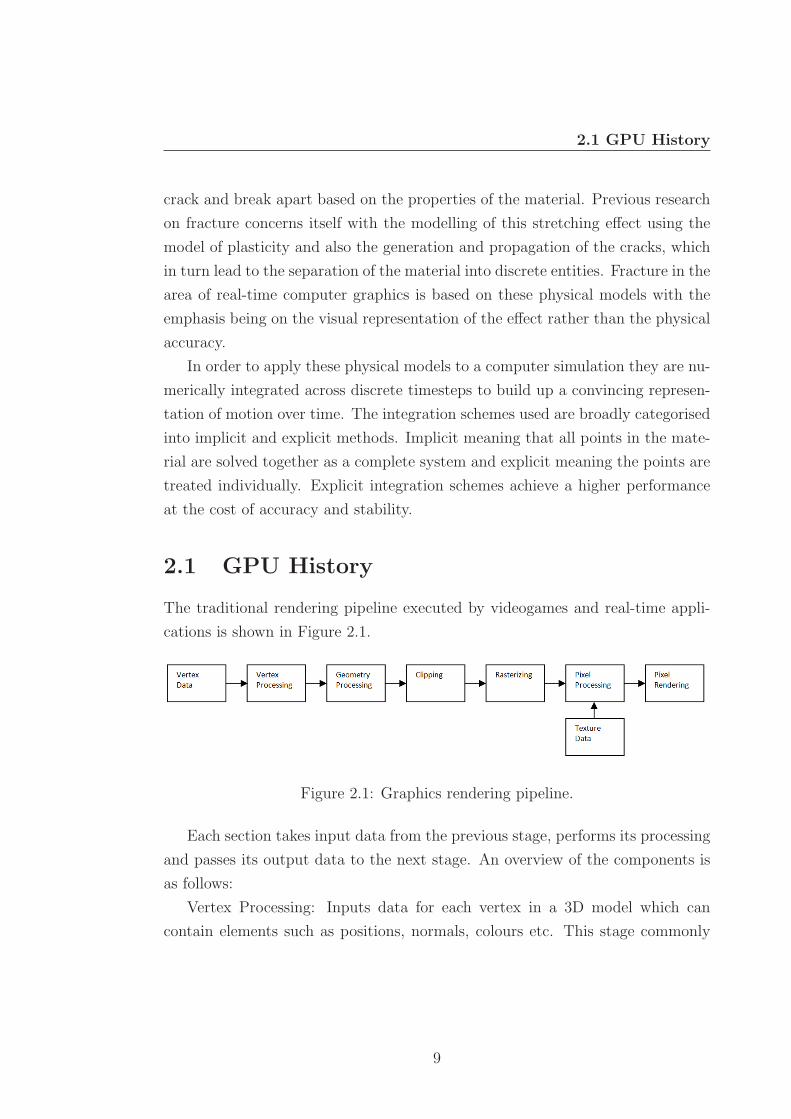
The traditional rendering pipeline executed by videogames and real-time appli-

cations is shown in Figure 2.1.

Figure 2.1: Graphics rendering pipeline.

Each section takes input data from the previous stage, performs its processing

and passes its output data to the next stage. An overview of the components is

as follows:

Vertex Processing: Inputs data for each vertex in a 3D model which can

contain elements such as positions, normals, colours etc. This stage commonly

9

2.1 GPU History

performs a 3D transformation from model to clip space and performs per vertex

lighting calculations.

Geometry Processing: Inputs a number of vertices from the previous stage to

make up a geometrical primitive (e.g. 3 vertices for a triangle). This stage can

then perform per primitive operations such as calculating face normals or adding

or removing primitives. It then outputs primitives with positions in clip space.

Clipping: Inputs clip space primitives and clips them to the specified clip

coordinates and outputs clipped primitives that are in the range of the current

visible clipping area.

Rasterizing: A number of stages occur here that take the clipped primitives

as input and produce a set of pixels that cover the triangle to be rendered in

screen space.

Pixel Processing: The pixels to be rendered are input and colouring, texturing

and lighting processing happens before outputting the final pixel colour to be

rendered to the screen.

Pixel Rendering: The pixel colours to be rendered are input and based on

the current states required are combined with the colours already at that pixel

location in the buffer that is being drawn to.

The initial drive to develop dedicated graphics acceleration hardware was to

improve the performance of the rendering pipeline. This was achieved by per-

forming common tasks in hardware circuitry. In the mid 1990s, the backend

of the rendering pipeline began to be implemented in hardware essentially from

the Rasterizing stage to the Pixel Rendering stage. This was fairly rigid in im-

plementation with a limited number of control parameters available to modify

outputs.

In 1999, the first graphics card to support hardware vertex processing was

shipped by NVIDIA: the GeForce256 [Akenine-Moller et al. 2008]. Although the

majority of the rendering pipeline was now implemented in hardware, it was very

rigid when it came to the modification of the processing and was therefore dubbed

the ’fixed function’ pipeline.

As the hardware evolved during the early part of this century, key stages of the

graphics pipeline were replaced with fully programmable units. The first of these

to appear were the vertex and pixel shader units allowing much more flexibility

10

2.2 Deformation

with the processing of vertex and pixel data. Although a step forward, these

units were quite limited and only allowed a minimal number of assembly language

instructions to be run at any one time and operating on a small number of memory

registers. Over time the number of instructions and memory registers increased

to a point where much more processing could be done within the vertex and pixel

shader units but the assembly language programs were becoming unmanageable

due to their size and complexity.

A number of shading languages were developed to encapsulate some of the

underlying hardware complexity in the form of languages similar to the ’C’ pro-

gramming language such as HLSL [MSDN 2010b], Cg [NVIDIA 2010a] and GLSL

[Khronos 2010b]. These languages provided much more flexibility over the graph-

ics pipeline processing whilst allowing easier management and re-usability of the

code that drives it.

The most recent graphics hardware has moved on another step to implement

a number of new additions to the hardware capabilities. A programmable geom-

etry shader unit has been added that allows more control over the processing of

geometrical primitives. Stream out functionality [MSDN 2010g] allows the out-

put data from either the vertex shader or geometry shader stages to be re-routed

to an external buffer rather than progressing through the graphics pipeline. This

allows the ability to feed processed data back into the start of the pipeline to

setup a processing feedback loop. Finally, it is also now possible to output pixel

data from the pixel shader stage to a number of buffers simultaneously using

multiple render targets (MRT’s) [MSDN 2010c] allowing the ability to process

and output separate sets of pixel data in a single rendering pass.

2.2 Deformation

Much of the early research into applying elasticity theory to model deformable

objects in the field of computer graphics was described in [Terzopoulos et al.

1987]. The authors describe the analysis of deformation as the calculation of the

relative distances between all points within a solid volume. For this, a Partial

Differential Equation (PDE) is devised that represents the entire material in a

11

2.2 Deformation

continuous fashion. The PDE is made up of the internal forces due to the de-

formable body on one side balancing out the externally applied forces. The PDE

is then discretised by transforming this equation of motion into linked Ordinary

Differential Equations (ODE’s) that can be numerically evaluated at various ma-

terial locations to be ultimately mapped to individual positions on an object.

The discretisation method used in this instance is the Finite Difference Method

(FDM) that describes the material as a regular grid of nodes and evaluates the

ODE’s between these nodes. The numerical integration of this solution governs

the entire shape and movement of the material to be modelled.

[O’Brien and Hodgins 1999] and [O’Brien et al. 2002] go on to use an im-

provement to the method of discretisation in order to allow representation of

irregular shaped materials. The Finite Element Method (FEM) is used and the

material is split into tetrahedral shapes across its volume leading to the ODEs

being evaluated across the tetrahedral faces.

The FEM in relation to modelling deformation in real-time computer graphics

is explained thoroughly in [Muller et al. 2008] where a pseudocode implementation

for a simulation algorithm is supplied.

When comparing the previous research, it is possible to extract commonalities

in the mathematical methods used to form the basis of a deformation simulation.

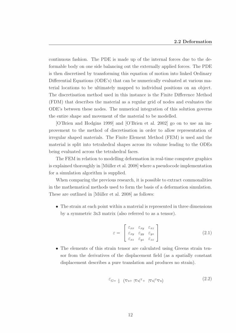
These are outlined in [Muller et al. 2008] as follows:

• The strain at each point within a material is represented in three dimensions

by a symmetric 3x3 matrix (also referred to as a tensor).

ε =

εxx εxy εxzεxy εyy εyzεxz εyz εzz

(2.1)

• The elements of this strain tensor are calculated using Greens strain ten-

sor from the derivatives of the displacement field (as a spatially constant

displacement describes a pure translation and produces no strain).

εG= 1

2 (∇u+ [∇u]T+ [∇u]T∇u) (2.2)

12

2.2 Deformation

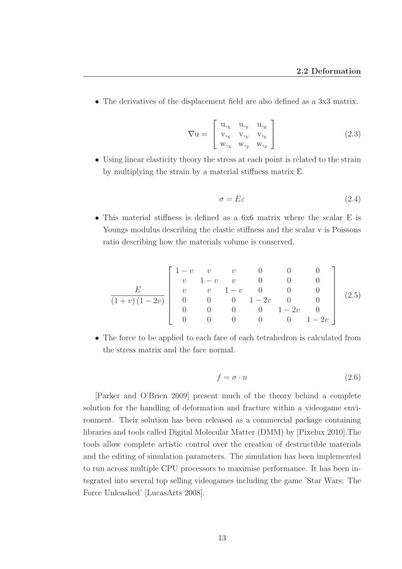
• The derivatives of the displacement field are also defined as a 3x3 matrix.

∇u =

u,x u,y u,zv,x v,y v,zw,x w,y w,z

(2.3)

• Using linear elasticity theory the stress at each point is related to the strain

by multiplying the strain by a material stiffness matrix E.

σ = Eε (2.4)

• This material stiffness is defined as a 6x6 matrix where the scalar E is

Youngs modulus describing the elastic stiffness and the scalar v is Poissons

ratio describing how the materials volume is conserved.

E

(1 + v) (1− 2v)

1− v v v 0 0 0v 1− v v 0 0 0v v 1− v 0 0 00 0 0 1− 2v 0 00 0 0 0 1− 2v 00 0 0 0 0 1− 2v

(2.5)

• The force to be applied to each face of each tetrahedron is calculated from

the stress matrix and the face normal.

f = σ · n (2.6)

[Parker and O’Brien 2009] present much of the theory behind a complete

solution for the handling of deformation and fracture within a videogame envi-

ronment. Their solution has been released as a commercial package containing

libraries and tools called Digital Molecular Matter (DMM) by [Pixelux 2010].The

tools allow complete artistic control over the creation of destructible materials

and the editing of simulation parameters. The simulation has been implemented

to run across multiple CPU processors to maximise performance. It has been in-

tegrated into several top selling videogames including the game ’Star Wars: The

Force Unleashed’ [LucasArts 2008].

13

2.3 Fracture

A particular implementation issue with deformation simulations that has been

raised by [Muller et al. 2008] and [Parker and O’Brien 2009] relates to an artefact

that occurs with the linear FEM under large rotational deformations. The prob-

lem is known as stiffness warping and occurs because current methods rely on

constant stiffness matrices that depend singularly on the rest configuration of the

simulated material in order to improve performance. The issue is addressed by

explicitly extracting the rotational part of the deformation and thus calculating

translations and rotations separately.

2.3 Fracture

[O’Brien and Hodgins 1999] introduce a method of analysing the stresses calcu-

lated in the deformation process by determining where cracks should begin and

how they should propagate throughout a simulated material. The model used is

based upon the theory of linear elastic fracture mechanics. At each point in the

material, a tensor is constructed describing the direction and size of the forces

acting to break apart the material at that location. When the forces exceed a

certain threshold, a fracture plane is computed perpendicular to the largest force

direction and the material is separated along this plane. The material is then re-

tessellated to fit along the crack edges. Over time, this has the effect of breaking

the material apart and propagating the crack throughout the material. In this

model the effects of plasticity before cracks appear are ignored and therefore it

is deemed as a model to simulate ’brittle’ materials whereby cracks have a ten-

dency to immediately appear after the stress threshold is reached and continue

to propagate thereafter.

In [O’Brien et al. 2002], the fracture model is refined to include the effects

of plasticity for materials that require it, and is dubbed ductile fracture. The

strain element of the deformation model is decomposed into two elements: the

strain due to plastic deformation and the strain due to elastic deformation. The

behaviour of the plasticity element is described by a yield value and a description

of plastic flow. Consequently, materials that exhibit ’ductile’ properties follow

elasticity principles up to the yield value, then stretch out of shape according

14

2.4 Numerical Integration

to the plasticity properties and finally crack and break apart upon reaching a

certain force threshold.

[Muller et al. 2001] describe the process of analysing the stresses from the

stress tensors calculated in the deformation process to supply the forces and

force directions at each material point. As a stress tensor is a 3x3 symmetric

matrix, it has three real eigenvalues. The eigenvalues correspond to the size of the

principal stresses and their eigenvectors to the principal stress directions. Positive

eigenvalues relate to tensile forces and negative eigenvalues to compressive forces.

The largest tensile eigenvalue is found for all tetrahedra in the material and

these are compared against the stress threshold. If the threshold is exceeded, all

tetrahedra within a set radius are divided either side of a fracture plane that is

perpendicular to the eigenvalues respective eigenvector.

2.4 Numerical Integration

In order to build a simulation representing the visual depiction of a deformable

and destructible material, each material point should obey Newton’s laws of mo-

tion. These laws of motion are numerically integrated at discrete timesteps which

leads to the update of the material points’ positions over time.

There are a number of numerical integration schemes available differing in

computational performance and accuracy of results. The two main categories are

implicit and explicit schemes with implicit meaning that all points in the material

are solved together as a complete system and explicit meaning the points are

treated individually. Within these categories there are various methods of varying

complexity and accuracy. The explicit schemes require much smaller timesteps

in order that the simulation does not become too unstable whereas the implicit

schemes are unconditionally stable but come with a higher computational cost.

The merits of various implicit and explicit numerical integration schemes for

the solution of a point based system are described in [Muller et al. 2008]. A

summary of these schemes are as follows:

15

2.4 Numerical Integration

• Explicit Integration Schemes

– Explicit Euler: the quantities for the next timestep are calculated

directly from the quantities at the current timestep using explicit for-

mulas.

– Runge Kutta: the forces are sampled multiple times within a timestep

in order to improve accuracy.

– Verlet: the quantities from the previous timestep and current timestep

are used to more accurately predict the quantities at the next timestep.

• Implicit Integration Schemes

– Implicit Euler: all positions and forces are combined into a single

system to be solved together.

– Newton Raphson: a solver used to solve the combined implicit Euler

scheme that works by iteratively guessing and refining future quanti-

ties.

16

Part II

Simulation

17

Chapter 3

Overview

A DirectX 10 and HLSL based material simulation prototype is described in

order to present this work. The areas of functionality developed are deformation

and fracture along with a method of defining the edges of destroyed materials

procedurally. These areas of functionality are broken down into the design of the

methods used along with their reasoning, and then the implementation details

specific to the chosen platform environment.

A number of decisions were made when approaching the overall design of

the simulation prototype in order to produce a clear and concise description of

the construction techniques used and also to maintain focus on the migration of

processing from the CPU to the GPU. A tetrahedral based FEM incorporating

the linear elasticity model is used that integrates motion using the explicit Euler

method, as these were found to be the most straight forward to implement and

most widely used throughout the research carried out. The effects of plasticity

and the issues of warping under large rotational deformations are ignored for the

purposes of this implementation as the solutions can become complex, therefore

plastic materials are not simulated and deformations are kept relatively small to

avoid these issues.

A framework is built that creates a wall made up of the simulated material

and displays this wall within a simple 3D scenario that allows the user to move

the camera around in order to view the simulation from different angles. A

graphical user interface (GUI) is provided with various options including the

ability to change the type of simulated material, switch between CPU or GPU

18

processing, and switch between the type of mesh to be displayed (simulation,

display, wireframe, solid).

A chapter is also provided covering some of the GPU best practices and tips

for implementation of the GPU algorithms detailed, drawn from the experience

gained whilst performing the required research to build the simulation prototype

(see Chapter 5).

19

Chapter 4

Framework

The simulation prototype was developed using Microsoft Visual Studio 2008 in-

tegrated development environment (IDE) and the C++ programming language.

The Microsoft DirectX software development kit (SDK) June 2010 was used as the

rendering application programming interface (API). The high level shading lan-

guage (HLSL) version 4.0 was used to create the shader code. These environment

and language choices were made as they are the most common throughout the

game development industry. The algorithms and methods developed throughout

this research could easily be adapted to other platforms and development envi-

ronments that have the appropriate API support to drive the graphics hardware.

In order to concentrate on the simulation prototype development and not

on areas such as creating display buffers, handling display setup and processing

mouse and keyboard input, the DirectX utility library (DXUT) [MSDN 2010a]

was used as a base for the application. The DXUT library also supplies useful

functionality such as allowing the device, multisample settings, and vsync options

to be changed at runtime. Also included is a graphical user interface (GUI)

framework that allows easy integration of custom GUI options. This was used

to good effect to supply user options to change material types, display options,

CPU / GPU processing and to reset the simulation whilst running.

The high level code framework for the wall to be displayed is broken down

into three sections called Wall, WallCPU and WallGPU. The Wall code contains

all of the initialisation, update and drawing code that is common amongst the

CPU and GPU implementations such as setting up node positions, finite element

20

structures and material parameters. The WallCPU and WallGPU code inherits

from the Wall code and extends the functionality to set up the specific parameters

and buffers required for either the CPU or GPU implementations. This layout

easily allows for configuring many walls and setting them to be either CPU or

GPU driven allowing for efficient system load balancing.

The runtime processing is set up with scene update and scene draw sections

that each run once per application update loop. The scene update section checks

for the appropriate key presses and mouse movement, updates the camera view

and applies forces to the wall at preset positions. It then runs the correct wall

update functionality based on whether it is configured for CPU or GPU process-

ing. The scene draw section clears the display buffer then draws the sky, ground

and wall to the same buffer.

21

Chapter 5

GPU Techniques Used

Whilst researching the current hardware GPU techniques available with DirectX

10 class graphics hardware for use in implementing the material simulation pro-

totype, a number of new GPU features were used as well as efficient methods of

utilising them. The following Section outlines these in more detail and provides

useful information for use within a variety of applications that wish to use GPU

hardware either as a generic stream processor or in the most efficient way possible

for graphics rendering purposes. Further best practices can be found in [NVIDIA

2008] and [Akenine-Moller et al. 2008].

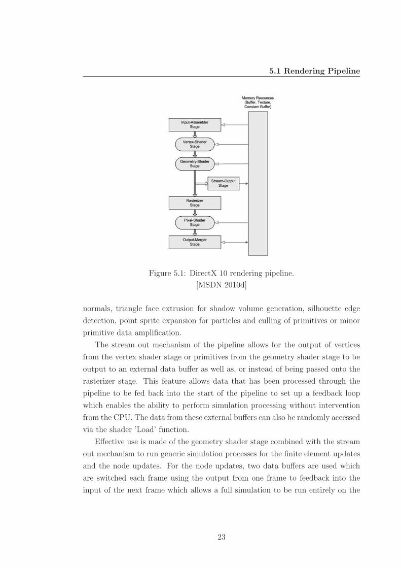
5.1 Rendering Pipeline

Referring to the DirectX 10 rendering pipeline shown in Figure 5.1, the geometry

shader is a programmable stage that sits between the vertex shader stage and the

rasterizer stage. Its purpose is to take a set of vertices from the vertex shader

as input, perform processing on a per primitive basis, whether that be points,

lines or triangles, and then output the results to the rasterizer. As well as the

primitive currently being operated on, it is possible to have information about the

adjacent primitives fed into the geometry shader in order to perform processing

such as edge detection algorithms. It is also possible to delete and add primitives

to the pipeline although the hardware is not designed for mass data amplification

so it is advised for this to be used sparingly to maintain reasonable performance.

Some common usages for the geometry shader include computing triangle face

22

5.1 Rendering Pipeline

Figure 5.1: DirectX 10 rendering pipeline.

[MSDN 2010d]

normals, triangle face extrusion for shadow volume generation, silhouette edge

detection, point sprite expansion for particles and culling of primitives or minor

primitive data amplification.

The stream out mechanism of the pipeline allows for the output of vertices

from the vertex shader stage or primitives from the geometry shader stage to be

output to an external data buffer as well as, or instead of being passed onto the

rasterizer stage. This feature allows data that has been processed through the

pipeline to be fed back into the start of the pipeline to set up a feedback loop

which enables the ability to perform simulation processing without intervention

from the CPU. The data from these external buffers can also be randomly accessed

via the shader ’Load’ function.

Effective use is made of the geometry shader stage combined with the stream

out mechanism to run generic simulation processes for the finite element updates

and the node updates. For the node updates, two data buffers are used which

are switched each frame using the output from one frame to feedback into the

input of the next frame which allows a full simulation to be run entirely on the

23

5.2 Optimisations

GPU. The details for each node are encapsulated into a single data structure and

rendered using a single point primitive per node. Harnessing this power allows

for many types of simulations to be run on the GPU in this manner effectively

utilising it as a generic stream processor. Some points worth mentioning here are

that streamout only supports the output of 32 bit data elements, therefore any

16 bit indices will need to be converted and using the ’SKIP’ semantic [MSDN

2010f] to omit data elements causes the PIX debugger tool, that is part of the

DirectX 10 SDK, to crash currently.

Multiple render targets (MRT’s) is another fairly recent technology that allows

the output of the pixel shader stage to be routed to more than one data buffer at

the same time. This feature enables the possibility of calculating separate areas

of a simulation simultaneously and storing their results in different data buffers

for later use. This is used to good effect in the fracture stage of the simulation

prototype to calculate the forces and eigenvalues in the same render pass. By

utilising the geometry shader output in clever ways, it is possible to output data

to different data locations and at varying frequencies into the separate output

data buffers.

5.2 Optimisations

Whilst taking advantage of some of these newer technologies, it is imperative to

perform optimisations with the usage of the API in order to maintain acceptable

performance levels to allow an application to perform well within a real-time

environment. At a high level, the overall goal in order to improve performance is

to pass less data through the graphics pipeline, i.e. to reduce the data bandwidth

requirements and to have less data that needs to be processed. Important aspects

to keep in mind when moving towards this goal are as follows:

• Describe vertex input data structures that are to be passed into the graph-

ics pipeline with the fewest number of bytes possible and also pack into

the native 32 bit x 4 data element widths. This will have the benefit of

reducing the memory bandwidth required to feed the input data into the

vertex shader. An example of this is the vertex structure used for the nodes

24

5.2 Optimisations

whereby the position takes up the xyz components of the first data element

and the x texture coordinate takes up the w component. Then similarly, the

velocity takes up the xyz components of the second data element and the

y texture coordinate takes up the w component. These data elements can

be easily unpacked in the vertex shader and reconstructed for their correct

usage.

• As with the vertex input data structures, it is desirable to pack data ele-

ments into as few components as possible into the vertex shader stage and

geometry shader stage output structures. This has the effect of reducing

the amount of work that the interpolator hardware has to perform when

interpolating data from primitives into pixels for the pixel shader stage to

consume.

• Always perform processing calculations at the earliest stage possible within

the graphics pipeline. In order to run calculations as few times as possi-

ble, processing them in the vertex or geometry shader stages will result in

them being run fewer times than in the pixel shader stage (assuming the

elements being processed are larger in size than a pixels dimensions). In

a graphics rendering setup, an example of this could be performing some

of the lighting calculations per vertex rather than per pixel. In a generic

stream processing setup, this could take the form of using point primitives

as the basic rendering element and performing all operations just once per

element in either the vertex or geometry shader stage as is done with the

finite element and node processing in the simulation prototype.

• If a texture is being read by one of the shader stages and then being written

to in a subsequent stage in a feedback loop, then any unused components

within the texture data elements can be used for additional storage rather

than passing them in via vertex data elements. The blend mode can then

be setup in such as way so that this extra data is preserved when writing

back out to the texture. An example of this can be seen in the node forces

used in the simulation prototype where the force per node is read from and

written to the RGB components of each texel in a 1D texture and the alpha

25

5.2 Optimisations

channel is used to store the inverse mass of each node. With alpha writes

turned off the inverse mass value is preserved and this saves storing the

value within the node structure itself.

• Minimise vertex shader, geometry shader and pixel shader processing. One

way this can be achieved is by storing the results of complex calculations in

textures as arrays of precomputed results and then looking up the required

result via a texture read rather than performing the calculation at run-time.

Other methods include using half precision 16 bit data element formats

where the full range of a 32 bit element is not required for the calculation

and hiding texture fetch latency by performing non dependent operations

after the texture reads.

• Reduce pixel fill rate requirements by switching on back face culling where

possible and using the lowest filtering and mipmap settings that produce

an acceptable visual result.

• Miscellaneous best practices are reducing the amount of pipeline state

changes as much as possible and not generating a large amount of primitives

from the geometry shader stage.

26

Chapter 6

Deformation

6.1 Method

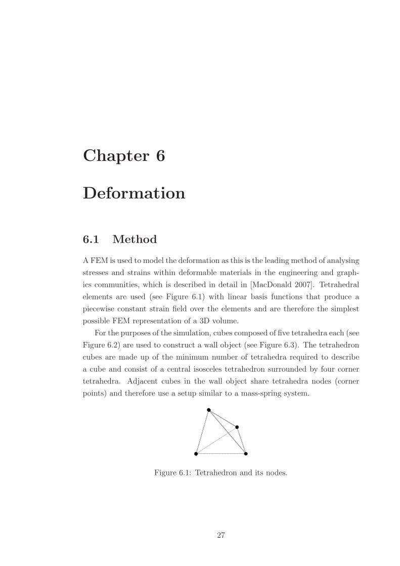
A FEM is used to model the deformation as this is the leading method of analysing

stresses and strains within deformable materials in the engineering and graph-

ics communities, which is described in detail in [MacDonald 2007]. Tetrahedral

elements are used (see Figure 6.1) with linear basis functions that produce a

piecewise constant strain field over the elements and are therefore the simplest

possible FEM representation of a 3D volume.

For the purposes of the simulation, cubes composed of five tetrahedra each (see

Figure 6.2) are used to construct a wall object (see Figure 6.3). The tetrahedron

cubes are made up of the minimum number of tetrahedra required to describe

a cube and consist of a central isosceles tetrahedron surrounded by four corner

tetrahedra. Adjacent cubes in the wall object share tetrahedra nodes (corner

points) and therefore use a setup similar to a mass-spring system.

Figure 6.1: Tetrahedron and its nodes.

27

6.1 Method

Figure 6.2: Cube composed of five tetrahedra.

Figure 6.3: Wall composed of tetrahedron cubes.

For maximum performance, the deformation simulation is split into two up-

date stages: updating the finite elements and updating the nodes. Using this

method ensures that each finite element and each node are processed only once.

The alternative would be to update each finite element in turn along with its as-

sociated four nodes in a single stage, but using such a configuration would mean

that shared nodes would be updated multiple times (although this would save

the storage space of the texture that accumulates the forces, so this is a speed

versus storage trade-off).

After any external forces are applied to the nodes, the finite element update

stage calculates the internal stresses and strains across the tetrahedron’s faces

and produces the internal forces to be applied to each node. The node update

stage then applies the internal forces to update the node velocities and positions

and integrates them over time to simulate the correct motion for the deformable

material.

The finite element update stage incorporates the FEM simulation formula and

processes each finite element tetrahedra as follows:

• Get the four node positions of the tetrahedra.

28

6.2 Implementation

• Calculate the derivatives of the displacement field from the node positions.

• Calculate Green’s strain tensor.

• Stress equals the material stiffness matrix times the strain.

• For each tetrahedron face, force equals stress times the face normal.

• Distribute tetrahedra face forces across tetrahedra nodes.

The node update stage processes each node as follows:

• Acceleration equals the force divided by the mass.

• Add gravity to the acceleration.

• Update the velocity by the time step times the acceleration.

• Update the position by the time step times the velocity.

• Add damping to the velocity.

The updated finite elements and nodes are then used in a draw stage to output

the simulation results to the display buffer.

6.2 Implementation

The finite elements and nodes are represented in as compact form as possible in

order to minimise memory bandwidth usage. Where appropriate, variables are

packed into float4 types to improve performance as suggested in [NVIDIA 2008].

Finite Element Structure:

short sIndex[4]; // indices into node list for the 4 nodes of this tetrahedron.

float3 matX[3]; // the 3x3 rest configuration matrix.

Node Structure:

29

6.2 Implementation

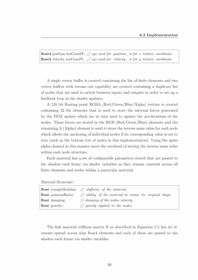
float4 position texCoordX; // xyz used for position , w for x texture coordinate.

float4 velocity texCoordY; // xyz used for velocity , w for y texture coordinate.

A single vertex buffer is created containing the list of finite elements and two

vertex buffers with stream out capability are created containing a duplicate list

of nodes that are used to switch between inputs and outputs in order to set up a

feedback loop in the shader updates.

A 128 bit floating point RGBA (Red/Green/Blue/Alpha) texture is created

containing 32 bit elements that is used to store the internal forces generated

by the FEM update which are in turn used to update the accelerations of the

nodes. These forces are stored in the RGB (Red/Green/Blue) elements and the

remaining A (Alpha) element is used to store the inverse mass value for each node

which allows the anchoring of individual nodes if its corresponding value is set to

zero (such as the bottom row of nodes in this implementation). Using the spare

alpha channel in this manner saves the overhead of storing the inverse mass value

within each node structure.

Each material has a set of configurable parameters stored that are passed to

the shaders each frame via shader variables as they remain constant across all

finite elements and nodes within a particular material.

Material Structure:

float youngsModulus; // stiffness of the material.

float poissonsRatio; // ability of the material to retain its original shape.

float damping; // damping of the nodes velocity .

float gravity ; // gravity applied to the nodes.

The 6x6 material stiffness matrix E as described in Equation 2.5 has its el-

ements spread across nine float4 elements and each of these are passed to the

shaders each frame via shader variables.

30

6.2 Implementation

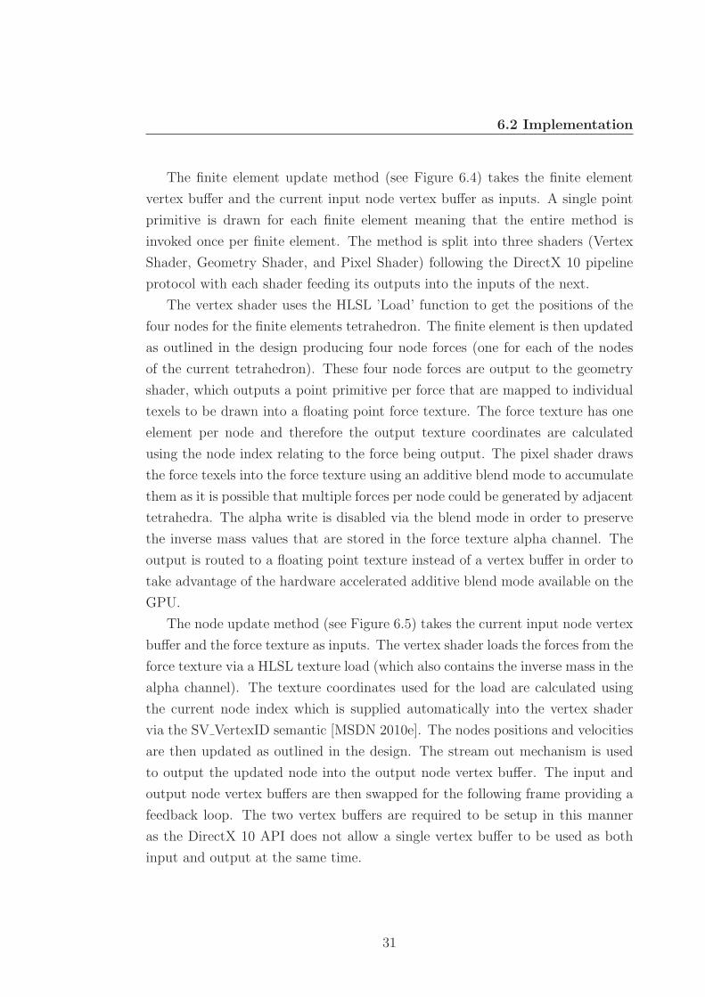
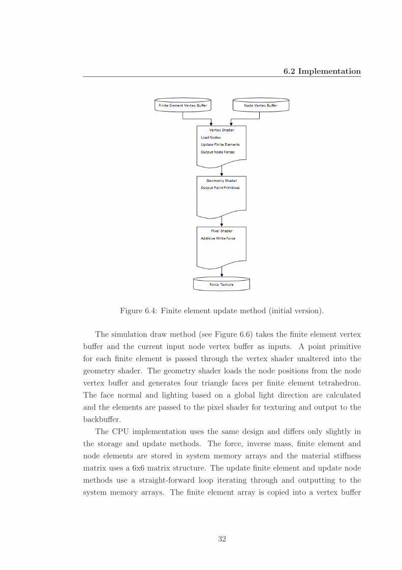
The finite element update method (see Figure 6.4) takes the finite element

vertex buffer and the current input node vertex buffer as inputs. A single point

primitive is drawn for each finite element meaning that the entire method is

invoked once per finite element. The method is split into three shaders (Vertex

Shader, Geometry Shader, and Pixel Shader) following the DirectX 10 pipeline

protocol with each shader feeding its outputs into the inputs of the next.

The vertex shader uses the HLSL ’Load’ function to get the positions of the

four nodes for the finite elements tetrahedron. The finite element is then updated

as outlined in the design producing four node forces (one for each of the nodes

of the current tetrahedron). These four node forces are output to the geometry

shader, which outputs a point primitive per force that are mapped to individual

texels to be drawn into a floating point force texture. The force texture has one

element per node and therefore the output texture coordinates are calculated

using the node index relating to the force being output. The pixel shader draws

the force texels into the force texture using an additive blend mode to accumulate

them as it is possible that multiple forces per node could be generated by adjacent

tetrahedra. The alpha write is disabled via the blend mode in order to preserve

the inverse mass values that are stored in the force texture alpha channel. The

output is routed to a floating point texture instead of a vertex buffer in order to

take advantage of the hardware accelerated additive blend mode available on the

GPU.

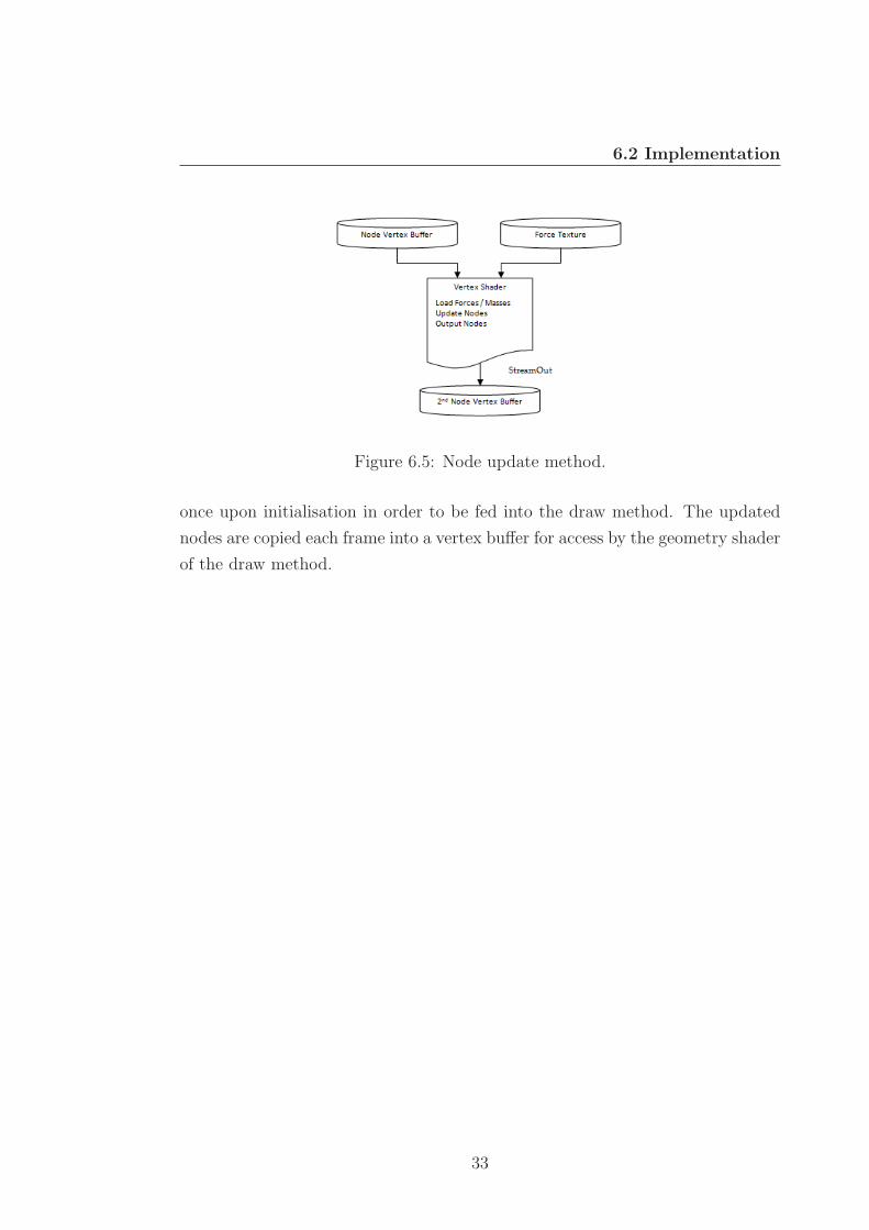
The node update method (see Figure 6.5) takes the current input node vertex

buffer and the force texture as inputs. The vertex shader loads the forces from the

force texture via a HLSL texture load (which also contains the inverse mass in the

alpha channel). The texture coordinates used for the load are calculated using

the current node index which is supplied automatically into the vertex shader

via the SV VertexID semantic [MSDN 2010e]. The nodes positions and velocities

are then updated as outlined in the design. The stream out mechanism is used

to output the updated node into the output node vertex buffer. The input and

output node vertex buffers are then swapped for the following frame providing a

feedback loop. The two vertex buffers are required to be setup in this manner

as the DirectX 10 API does not allow a single vertex buffer to be used as both

input and output at the same time.

31

6.2 Implementation

Figure 6.4: Finite element update method (initial version).

The simulation draw method (see Figure 6.6) takes the finite element vertex

buffer and the current input node vertex buffer as inputs. A point primitive

for each finite element is passed through the vertex shader unaltered into the

geometry shader. The geometry shader loads the node positions from the node

vertex buffer and generates four triangle faces per finite element tetrahedron.

The face normal and lighting based on a global light direction are calculated

and the elements are passed to the pixel shader for texturing and output to the

backbuffer.

The CPU implementation uses the same design and differs only slightly in

the storage and update methods. The force, inverse mass, finite element and

node elements are stored in system memory arrays and the material stiffness

matrix uses a 6x6 matrix structure. The update finite element and update node

methods use a straight-forward loop iterating through and outputting to the

system memory arrays. The finite element array is copied into a vertex buffer

32

6.2 Implementation

Figure 6.5: Node update method.

once upon initialisation in order to be fed into the draw method. The updated

nodes are copied each frame into a vertex buffer for access by the geometry shader

of the draw method.

33

6.2 Implementation

Figure 6.6: Simulation draw method.

34

Chapter 7

Fracture

7.1 Method

A process similar to that described in [Muller et al. 2001] is used to compute the

maximum eigenvalue for each finite element in the simulation. The eigenvalues

are compared against the maximum stress threshold set for the current material

to determine where cracks should occur. Each tetrahedron based cube is broken

away from the rest of the wall structure in its entirety rather than splitting and

retesselating at run-time in order to maximise performance and to allow a GPU

implementation.

Whilst designing the GPU method for fracture, it became apparent that du-

plicating shared nodes where the tetrahedron based cubes meet each other under

a GPU stream processing architecture would be impossible to implement. This

is due to the fact that the finite elements and nodes are processed individually

using streams of data as their input, rather than having the access to random

elements available within a CPU implementation. The possibility of using the

geometry shader’s ability to output varying numbers of primitives to its output

buffer was investigated but if the number of nodes in the vertex buffer were to

be altered then the node indices stored within each finite element would need to

be adjusted. A workable solution that maintains a high level of performance (in

terms of execution speed) was not found.

In order to solve this problem, a novel solution of changing the underlying

structure for the connectivity of the nodes fed into the deformation system is

35

7.2 Implementation

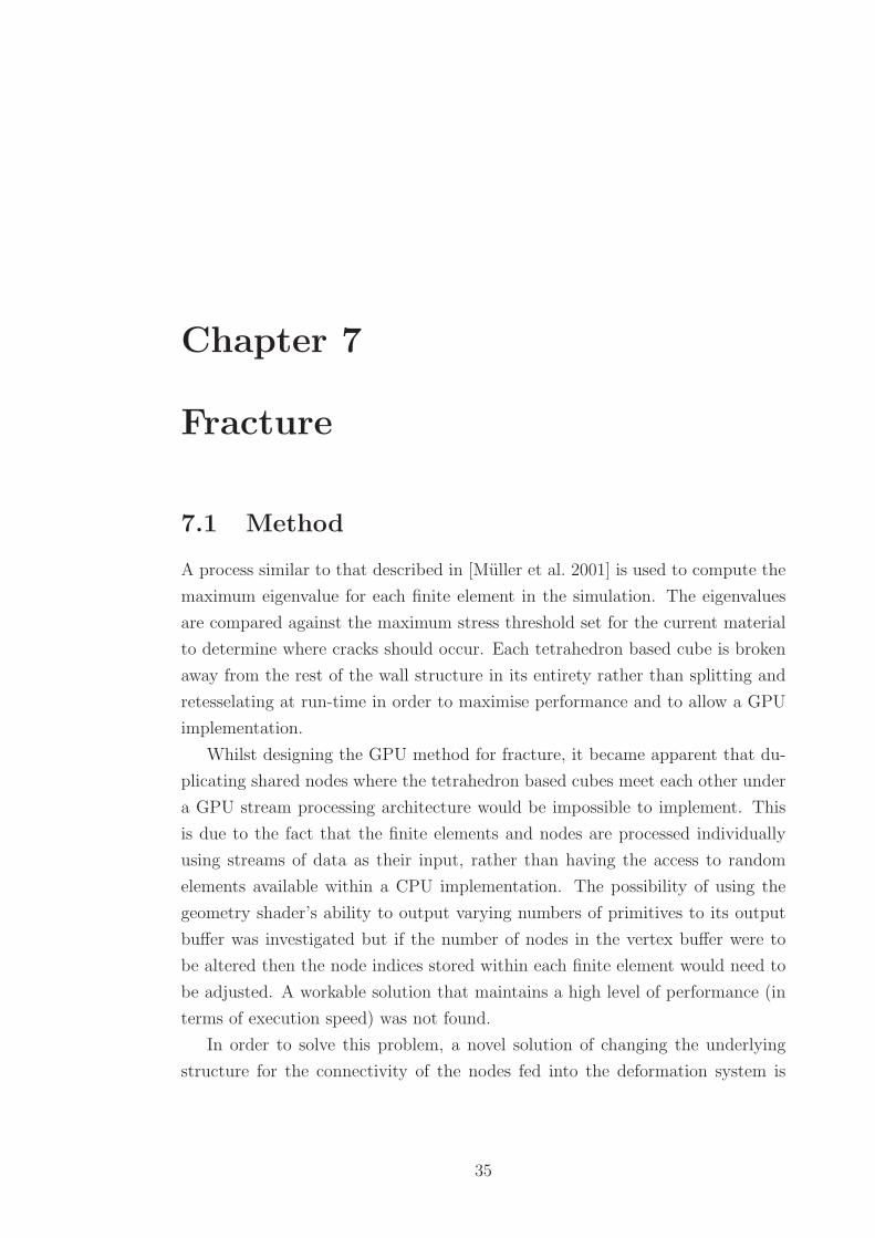
presented. Instead of the finite element based cubes being connected to the nodes

in a sharing fashion similar to a mass-spring system, each tetrahedron based cube

has its own unique eight corner nodes (see Figure 7.1).

Figure 7.1: New finite element connectivity.

To maintain a consistent state when updating the deformation simulation, a

separate list of connections are stored for the eight corner nodes detailing the

other corner nodes that each corner is currently connected to. After the forces

are calculated in the deformation pass, another pass is run that accumulates each

force based on its current connections.

With the simulation set up in this manner, it is possible to flag a finite ele-

ment as being disconnected whilst processing the individual finite element in the

GPU vertex shader without having to duplicate any nodes at run-time. When

a finite element’s corner node is flagged as disconnected, its forces are no longer

accumulated with its neighbours and therefore it begins to separate itself from

the adjacent elements.

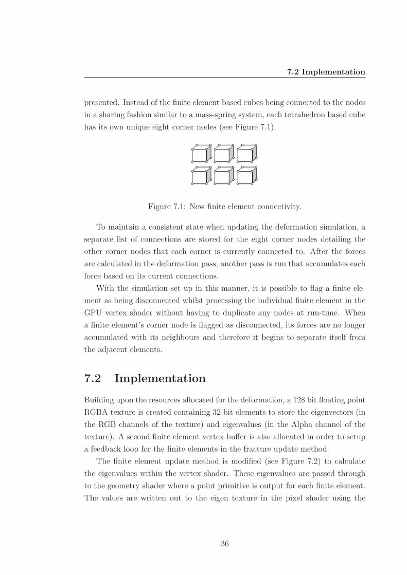
7.2 Implementation

Building upon the resources allocated for the deformation, a 128 bit floating point

RGBA texture is created containing 32 bit elements to store the eigenvectors (in

the RGB channels of the texture) and eigenvalues (in the Alpha channel of the

texture). A second finite element vertex buffer is also allocated in order to setup

a feedback loop for the finite elements in the fracture update method.

The finite element update method is modified (see Figure 7.2) to calculate

the eigenvalues within the vertex shader. These eigenvalues are passed through

to the geometry shader where a point primitive is output for each finite element.

The values are written out to the eigen texture in the pixel shader using the

36

7.2 Implementation

multiple render target (MRT) technology. The output texture coordinates are

calculated using the automatically supplied SV VertexID semantic [MSDN 2010e]

and therefore output to different locations than the output force values within

the same geometry shader.

Figure 7.2: Finite element update method (extended version).

The material structure is modified to add a maximum stress value for the

current material being simulated:

Material Structure:

...

float maxStress; // compared with the eigenvalue to determine fracture.

...

37

7.2 Implementation

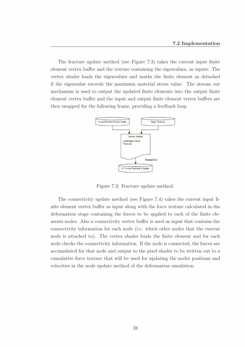
The fracture update method (see Figure 7.3) takes the current input finite

element vertex buffer and the texture containing the eigenvalues, as inputs. The

vertex shader loads the eigenvalues and marks the finite element as detached

if the eigenvalue exceeds the maximum material stress value. The stream out

mechanism is used to output the updated finite elements into the output finite

element vertex buffer and the input and output finite element vertex buffers are

then swapped for the following frame, providing a feedback loop.

Figure 7.3: Fracture update method.

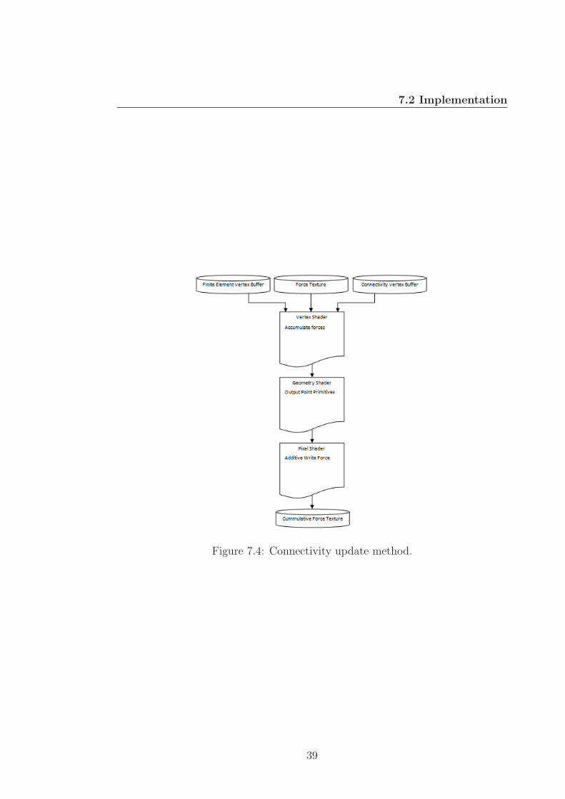
The connectivity update method (see Figure 7.4) takes the current input fi-

nite element vertex buffer as input along with the force texture calculated in the

deformation stage containing the forces to be applied to each of the finite ele-

ments nodes. Also a connectivity vertex buffer is used as input that contains the

connectivity information for each node (i.e. which other nodes that the current

node is attached to). The vertex shader loads the finite element and for each

node checks the connectivity information. If the node is connected, the forces are

accumulated for that node and output to the pixel shader to be written out to a

cumulative force texture that will be used for updating the nodes positions and

velocities in the node update method of the deformation simulation.

38

7.2 Implementation

Figure 7.4: Connectivity update method.

39

Chapter 8

Procedural Edges

8.1 Method

For providing interesting detail to the edges of fractured materials, some influence

is taken from the work done by [Scheepers and Whittock 2006] where sections

of geometry are precomputed to contain broken edge detail and fitted together

perfectly so as to look undamaged in its initial state.

A separate display mesh is created, each section of which relates to one tetra-

hedral cube within the simulation mesh. The vertex positions of the display

mesh are linked to the finite elements in the simulation mesh using barycentric

coordinates, allowing the display mesh movement to mirror the simulation mesh

movement in real time.

To create the look and feel of a destroyed material when the sections are

fractured, two novel solutions are provided. The width and height of the sections

are adjusted by a random factor and also linked to a material parameter to

allow for user control. Also, a number of vertices are randomly placed along

each section edge and joined up with polygons to the edge. These two elements

combined provide the possibility of simulating a wide range of material types by

adjusting the material parameters.

As there are some random number factors involved with the generation of

the display mesh, each time a mesh is initialised, it will be constructed slightly

differently, despite the fact that they are obeying the material parameters of the

40

8.2 Implementation

selected material type. This means that each time a material is broken apart, it

looks and acts differently even though the display mesh was precomputed.

As all of the calculations for generating the display mesh are performed in the

initialisation stage, it was felt that it was sufficient to perform this task on the

CPU, which would not justify the effort to attempt to construct the mesh using

GPU methods.

8.2 Implementation

The material structure is expanded to include parameters to control the look of

the precomputed display mesh as follows:

Material Structure:

...

float avgDisplaySectionWidth; // width of sections before random factor.

float avgDisplaySectionHeight; // height of sections before random factor.

float randDisplaySectionWidth; // random width factor to be added to sections .

float randDisplaySectionHeight; // random height factor to be added to sections .

float horizEdgeFrequency; // number of edge points to be added horizontally .

float horizEdgeAmplitude; // size of added horizontal edge polygons.

float vertEdgeFrequency; // number of edge points to be added vertically .

float vertEdgeAmplitude; // size of added vertical edge polygons.

...

The display mesh is initially created with section sizes based on the materials

avgDisplaySectionWidth and avgDisplaySectionHeight parameters divided into

the requested width and height of the entire wall. These parameters are called

averages because they are first divided into the walls dimensions then adjusted

to have evenly spaced sections.

For each section, all edges apart from those on the perimeter of the wall are

adjusted based on the randDisplaySectionWidth and randDisplaySectionHeight

41

8.2 Implementation

material parameters. This has the effect of breaking up the uniform layout of the

walls geometry and also creating a different layout each time the wall is initialised.

For each of the horizontal and vertical edges of each section excluding those

around the walls perimeter, a number of vertices are inserted based on the

horizEdgeFrequency and vertEdgeFrequency material parameters. These are used

to create polygon edges that stitched into the existing sections with their size

based on the horizEdgeAmplitude and vertEdgeAmplitude material parameters.

Using different variations of material parameters along with a suitable display

texture, the wall in the simulation prototype can be made to resemble the in-

tended material quite closely. For example, using roughly square shaped sections

with few edge vertices can give the impression of a glass window when broken

apart. Using long thin sections without vertical edge vertices but with many

horizontal edge vertices at a high amplitude gives the effect of planks of wood

being broken with sharp splinter type edges.

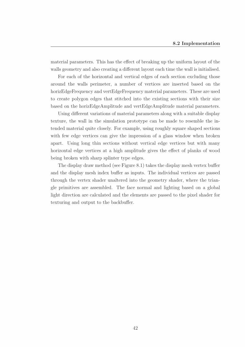
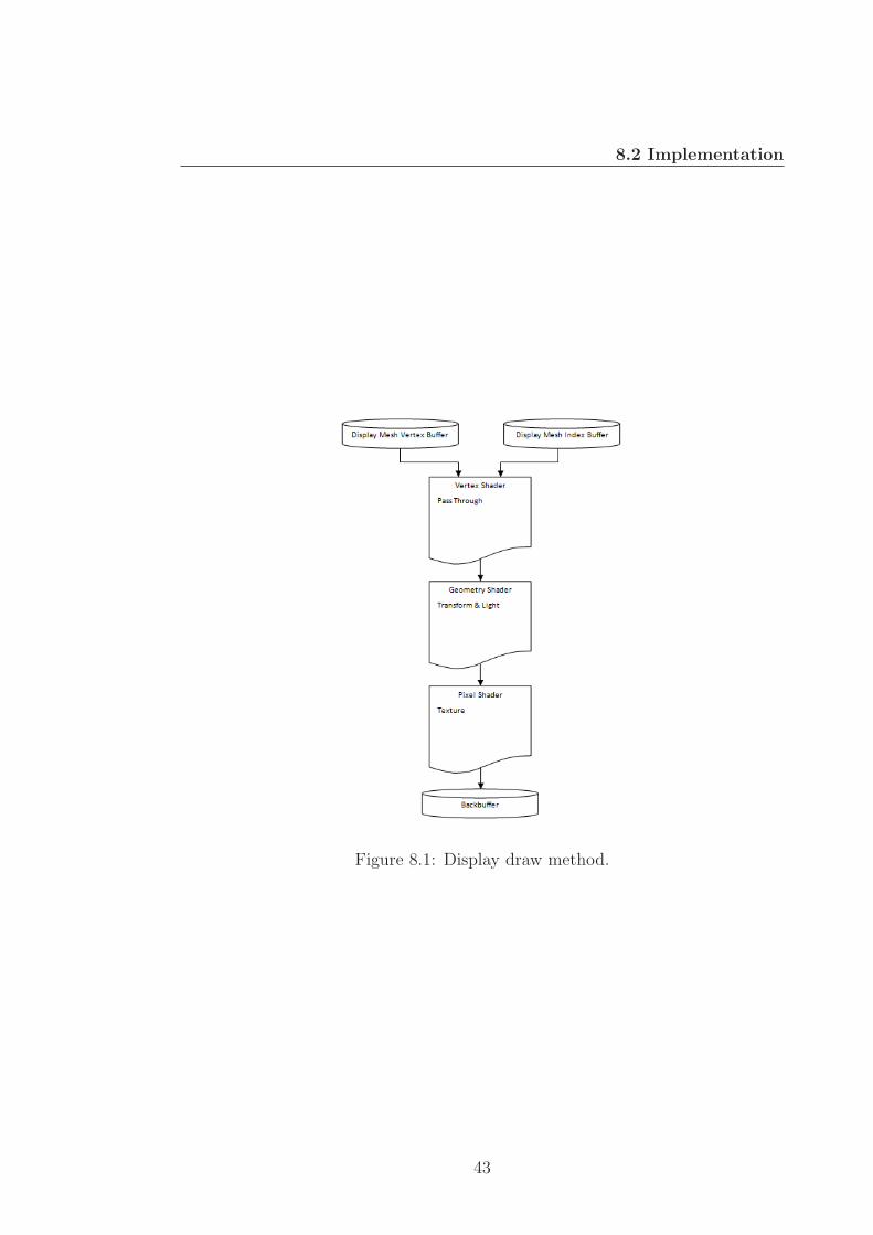
The display draw method (see Figure 8.1) takes the display mesh vertex buffer

and the display mesh index buffer as inputs. The individual vertices are passed

through the vertex shader unaltered into the geometry shader, where the trian-

gle primitives are assembled. The face normal and lighting based on a global

light direction are calculated and the elements are passed to the pixel shader for

texturing and output to the backbuffer.

42

8.2 Implementation

Figure 8.1: Display draw method.

43

Part III

Conclusions

44

Chapter 9

Results and Discussion

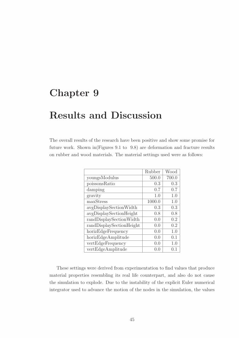
The overall results of the research have been positive and show some promise for

future work. Shown in(Figures 9.1 to 9.8) are deformation and fracture results

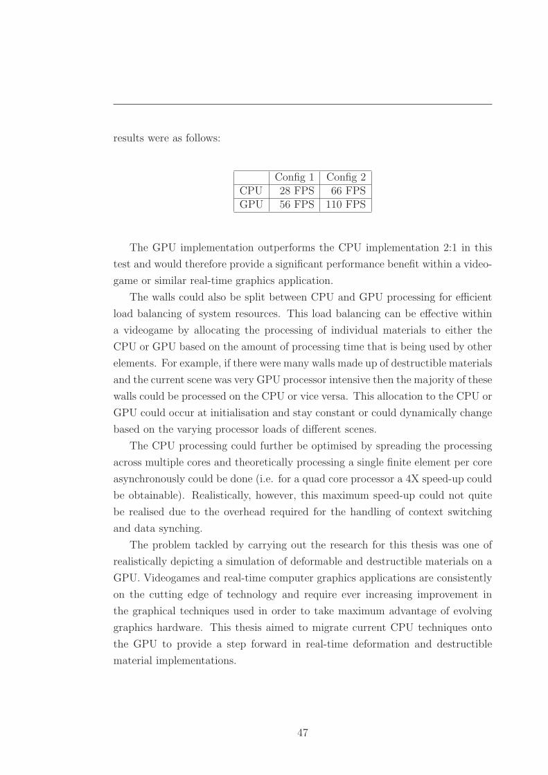
on rubber and wood materials. The material settings used were as follows:

Rubber WoodyoungsModulus 500.0 700.0poissonsRatio 0.3 0.3damping 0.7 0.7gravity 1.0 1.0maxStress 1000.0 1.0avgDisplaySectionWidth 0.3 0.3avgDisplaySectionHeight 0.8 0.8randDisplaySectionWidth 0.0 0.2randDisplaySectionHeight 0.0 0.2horizEdgeFrequency 0.0 1.0horizEdgeAmplitude 0.0 0.1vertEdgeFrequency 0.0 1.0vertEdgeAmplitude 0.0 0.1

These settings were derived from experimentation to find values that produce

material properties resembling its real life counterpart, and also do not cause

the simulation to explode. Due to the instability of the explicit Euler numerical

integrator used to advance the motion of the nodes in the simulation, the values

45

shown above can only be varied approximately ±50% before the simulation ex-

plodes, i.e. becomes unstable, and therefore only a small range of material types

can be simulated without integrator improvements. The rubber material has a

high stress threshold set so that it deforms out of shape and does not break apart.

The wood material has a low stress threshold and higher youngsModulus which

causes the fracture to occur quickly without deforming out of shape much. The

wood material also has settings for the horizontal and vertical edges that control

the look of the edges when broken apart.

As a performance test, a test scene was set up containing fifty walls (see Fig-

ure 9.9) and the simulation was run on two separate PC configurations (a low

end laptop and a high end desktop). As the processing carried out is the same

regardless of material type and the amount of processing scales linearly with the

number of walls in the scene, it was felt that supplying FPS results for different

materials and/or size of walls would be redundant.

Configuration 1:

Operating system: Windows 7 Home Premium

Microsoft Windows rating: 5.7

Processor: Intel(R) Core(TM)2 Duo CPU P7450 @ 2.13GHz

Installed memory (RAM): 4.00 GB

System type: 64-bit Operating System

Graphics: NVIDIA GeForce GT 230M

Configuration 2:

Operating system: Windows 7 Enterprise

Microsoft Windows rating: 6.2

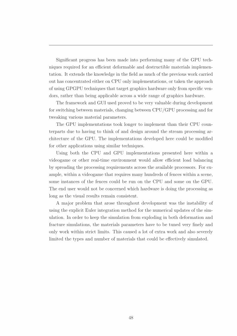
Processor: Intel(R) Core(TM) i7 CPU 920 @ 2.66GHz

Installed memory (RAM): 8.00 GB

System type: 64-bit Operating System

Graphics: ATI Radeon HD 4870 X2

Each wall contains 270 finite elements and 152 nodes giving a total of 13500

finite elements and 7600 nodes for the 50 walls. The frames per second (FPS)

46

results were as follows:

Config 1 Config 2CPU 28 FPS 66 FPSGPU 56 FPS 110 FPS

The GPU implementation outperforms the CPU implementation 2:1 in this

test and would therefore provide a significant performance benefit within a video-

game or similar real-time graphics application.

The walls could also be split between CPU and GPU processing for efficient

load balancing of system resources. This load balancing can be effective within

a videogame by allocating the processing of individual materials to either the

CPU or GPU based on the amount of processing time that is being used by other

elements. For example, if there were many walls made up of destructible materials

and the current scene was very GPU processor intensive then the majority of these

walls could be processed on the CPU or vice versa. This allocation to the CPU or

GPU could occur at initialisation and stay constant or could dynamically change

based on the varying processor loads of different scenes.

The CPU processing could further be optimised by spreading the processing

across multiple cores and theoretically processing a single finite element per core

asynchronously could be done (i.e. for a quad core processor a 4X speed-up could

be obtainable). Realistically, however, this maximum speed-up could not quite

be realised due to the overhead required for the handling of context switching

and data synching.

The problem tackled by carrying out the research for this thesis was one of

realistically depicting a simulation of deformable and destructible materials on a

GPU. Videogames and real-time computer graphics applications are consistently

on the cutting edge of technology and require ever increasing improvement in

the graphical techniques used in order to take maximum advantage of evolving

graphics hardware. This thesis aimed to migrate current CPU techniques onto

the GPU to provide a step forward in real-time deformation and destructible

material implementations.

47

Significant progress has been made into performing many of the GPU tech-

niques required for an efficient deformable and destructible materials implemen-

tation. It extends the knowledge in the field as much of the previous work carried

out has concentrated either on CPU only implementations, or taken the approach

of using GPGPU techniques that target graphics hardware only from specific ven-

dors, rather than being applicable across a wide range of graphics hardware.

The framework and GUI used proved to be very valuable during development

for switching between materials, changing between CPU/GPU processing and for

tweaking various material parameters.

The GPU implementations took longer to implement than their CPU coun-

terparts due to having to think of and design around the stream processing ar-

chitecture of the GPU. The implementations developed here could be modified

for other applications using similar techniques.

Using both the CPU and GPU implementations presented here within a

videogame or other real-time environment would allow efficient load balancing

by spreading the processing requirements across the available processors. For ex-

ample, within a videogame that requires many hundreds of fences within a scene,

some instances of the fences could be run on the CPU and some on the GPU.

The end user would not be concerned which hardware is doing the processing as

long as the visual results remain consistent.

A major problem that arose throughout development was the instability of

using the explicit Euler integration method for the numerical updates of the sim-

ulation. In order to keep the simulation from exploding in both deformation and

fracture simulations, the materials parameters have to be tuned very finely and

only work within strict limits. This caused a lot of extra work and also severely

limited the types and number of materials that could be effectively simulated.

48

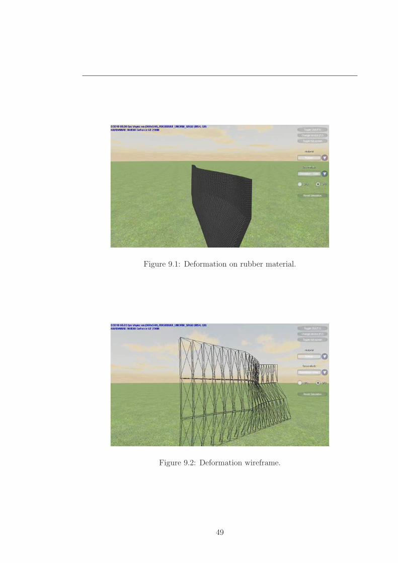
Figure 9.1: Deformation on rubber material.

Figure 9.2: Deformation wireframe.

49

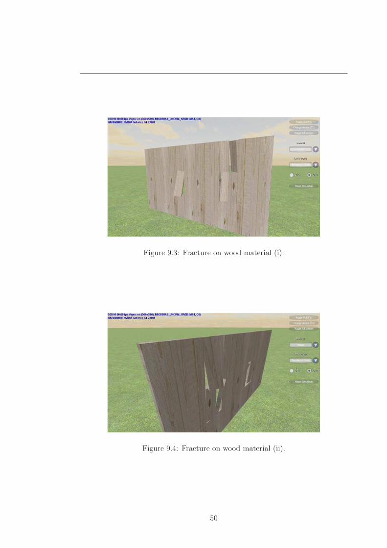
Figure 9.3: Fracture on wood material (i).

Figure 9.4: Fracture on wood material (ii).

50

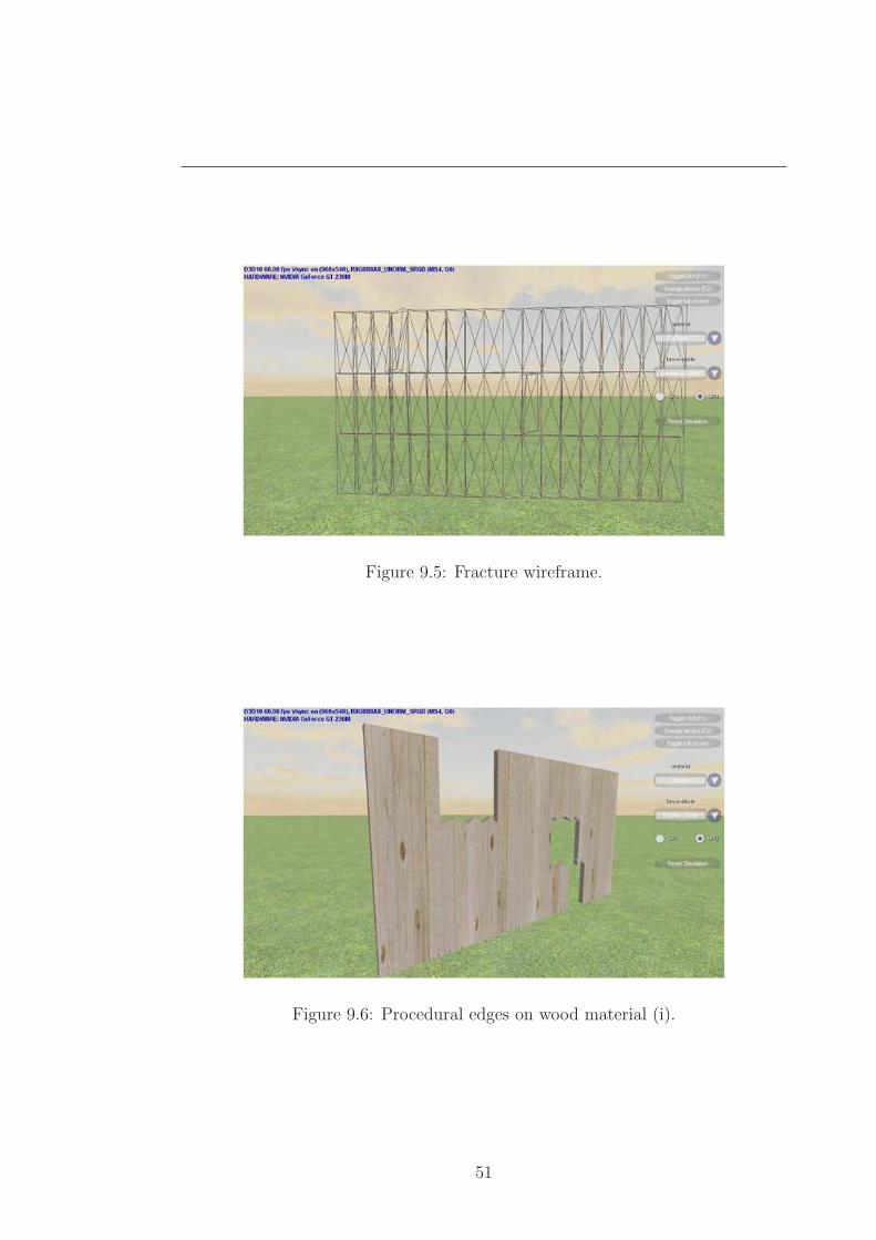
Figure 9.5: Fracture wireframe.

Figure 9.6: Procedural edges on wood material (i).

51

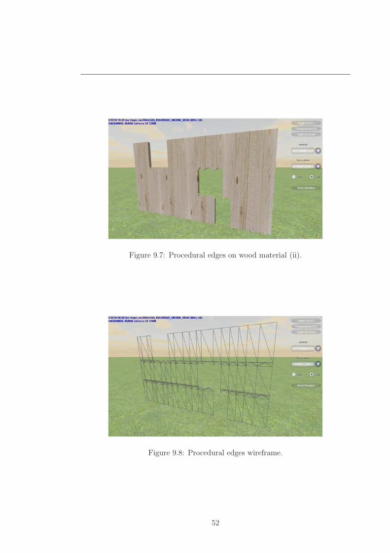
Figure 9.7: Procedural edges on wood material (ii).

Figure 9.8: Procedural edges wireframe.

52

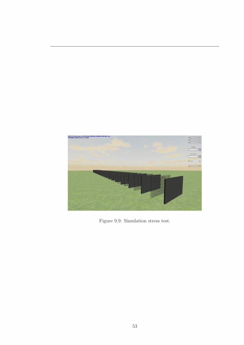
Figure 9.9: Simulation stress test.

53

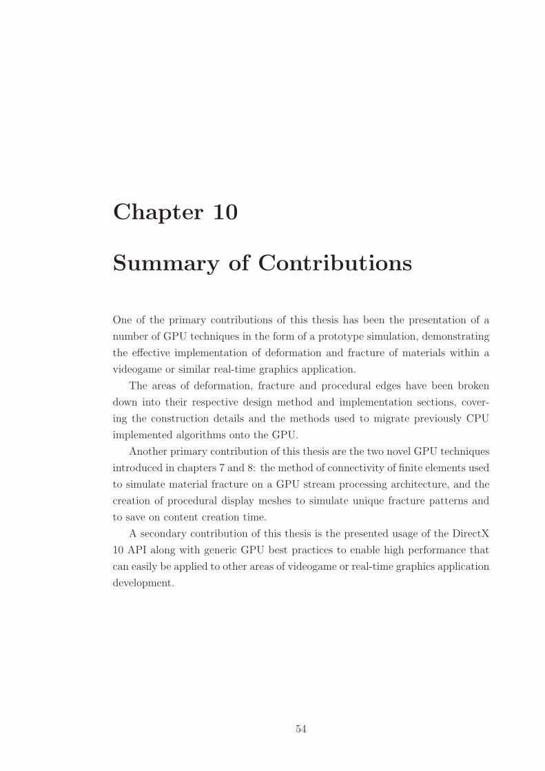
Chapter 10

Summary of Contributions

One of the primary contributions of this thesis has been the presentation of a

number of GPU techniques in the form of a prototype simulation, demonstrating

the effective implementation of deformation and fracture of materials within a

videogame or similar real-time graphics application.

The areas of deformation, fracture and procedural edges have been broken

down into their respective design method and implementation sections, cover-

ing the construction details and the methods used to migrate previously CPU

implemented algorithms onto the GPU.

Another primary contribution of this thesis are the two novel GPU techniques

introduced in chapters 7 and 8: the method of connectivity of finite elements used

to simulate material fracture on a GPU stream processing architecture, and the

creation of procedural display meshes to simulate unique fracture patterns and

to save on content creation time.

A secondary contribution of this thesis is the presented usage of the DirectX

10 API along with generic GPU best practices to enable high performance that

can easily be applied to other areas of videogame or real-time graphics application

development.

54

Chapter 11

Future Work

The biggest improvement that could be made to the prototype simulation de-

veloped within this research would be to implement a more advanced numerical

integration method such as the implicit Euler method. Although implementing

and integrating this into the GPU methods presented would be a considerable

task, it is felt that without this the methods presented here do not have enough

stability for use within a commercial environment.

The procedural edges methods presented here are a good start to providing an

automated system for producing the required edge geometry for fracture simula-

tion. These could be improved by introducing more complex parameter controls.

One such improvement could be having a step to the edges for materials such as

brick and matching these stepped edges with the material’s texture to provide a

convincing brick edge.

For a full deformation and fracture simulation, two methods of collisions would

need to be developed and integrated into the simulation: object to wall collisions

for external objects hitting the wall, and self collisions for broken wall sections

hitting other sections of the wall and the ground.

In order to implement these techniques into a commercial environment, it

would be desirable to produce an editor that loads geometry created by artists

and generates the appropriate finite element simulation geometry and display

meshes. Material parameters could be tweaked and simulated in real-time for a

fast turnaround time for setting up materials.

55

Throughout this thesis, the quality of the simulation presented has been mea-

sured by judging whether the output provides the perception of a realistic virtual

environment. This has been a judgement call based on the author’s experience

within the videogame industry. However, a more thorough investigation could be

carried out into this, similar to that presented in [O’Sullivan et al. 2003].

With future advances in GPU technology on the horizon, it should not only

be possible to simulate different material types that deform and fracture in a

visually plausible manner under real-time conditions with minimal intervention

by the CPU, but many of the used techniques could be implemented using GPU

methods and expressed in a more generic form with the intention of moving

towards having a fully GPU-based physical simulation of all aspects of the game

world.

56

Appendices

57

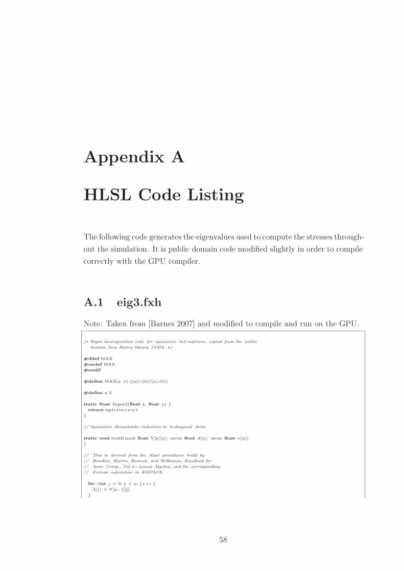
Appendix A

HLSL Code Listing

The following code generates the eigenvalues used to compute the stresses through-

out the simulation. It is public domain code modified slightly in order to compile

correctly with the GPU compiler.

A.1 eig3.fxh

Note: Taken from [Barnes 2007] and modified to compile and run on the GPU.

/∗ Eigen decomposition code for symmetric 3x3 matrices, copied from the public

domain Java Matrix library JAMA. ∗/

#ifdef MAX

#undef MAX

#endif

#define MAX(a, b) ((a)>(b)?(a):(b))

#define n 3

static float hypot2(float x, float y) {

return sqrt(x∗x+y∗y);

}

// Symmetric Householder reduction to tridiagonal form.

static void tred2(inout float V[n][n ], inout float d[n], inout float e[n])

{

// This is derived from the Algol procedures tred2 by

// Bowdler, Martin, Reinsch, and Wilkinson, Handbook for

// Auto. Comp., Vol.ii−Linear Algebra, and the corresponding

// Fortran subroutine in EISPACK.

for (int j = 0; j < n; j++) {

d[j ] = V[n−1][j];

}

58

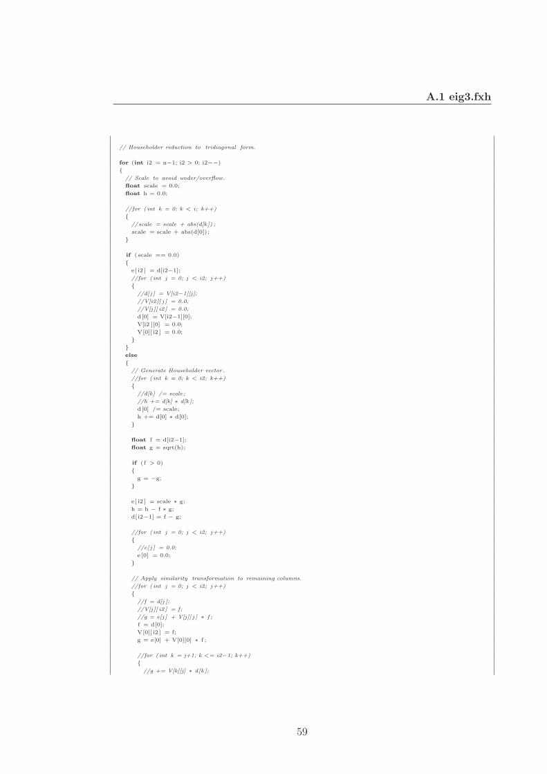
A.1 eig3.fxh

// Householder reduction to tridiagonal form.

for (int i2 = n−1; i2 > 0; i2−−)

{

// Scale to avoid under/overflow.

float scale = 0.0;

float h = 0.0;

//for ( int k = 0; k < i; k++)

{

//scale = scale + abs(d[k]) ;

scale = scale + abs(d[0]);

}

if (scale == 0.0)

{

e[ i2 ] = d[i2−1];

//for ( int j = 0; j < i2; j++)

{

//d[j ] = V[i2−1][j];

//V[i2][ j ] = 0.0;

//V[j ][ i2 ] = 0.0;

d[0] = V[i2−1][0];

V[i2 ][0] = 0.0;

V[0][ i2 ] = 0.0;

}

}

else

{

// Generate Householder vector.

//for ( int k = 0; k < i2; k++)

{

//d[k] /= scale;

//h += d[k] ∗ d[k ];

d[0] /= scale;

h += d[0] ∗ d[0];

}

float f = d[i2−1];

float g = sqrt(h);

if (f > 0)

{

g = −g;

}

e[ i2 ] = scale ∗ g;

h = h − f ∗ g;

d[i2−1] = f − g;

//for ( int j = 0; j < i2; j++)

{

//e[ j ] = 0.0;

e [0] = 0.0;

}

// Apply similarity transformation to remaining columns.

//for ( int j = 0; j < i2; j++)

{

//f = d[j ];

//V[j ][ i2 ] = f;

//g = e[j ] + V[j][ j ] ∗ f ;

f = d[0];

V[0][ i2 ] = f;

g = e[0] + V[0][0] ∗ f ;

//for ( int k = j+1; k <= i2−1; k++)

{

//g += V[k][j] ∗ d[k ];

59

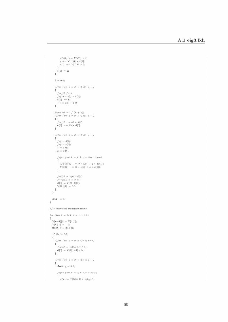
A.1 eig3.fxh

//e[k] += V[k][j] ∗ f ;

g += V[1][0] ∗ d[1];

e [1] += V[1][0] ∗ f ;

}

e [0] = g;

}

f = 0.0;

//for ( int j = 0; j < i2; j++)

{

//e[ j ] /= h;

//f += e[j] ∗ d[ j ];

e [0] /= h;

f += e[0] ∗ d[0];

}

float hh = f / (h + h);

//for ( int j = 0; j < i2; j++)

{

//e[ j ] −= hh ∗ d[j];

e [0] −= hh ∗ d[0];

}

//for ( int j = 0; j < i2; j++)

{

//f = d[j ];

//g = e[j ];

f = d[0];

g = e[0];

//for ( int k = j; k <= i2−1; k++)

{

//V[k][ j ] −= (f ∗ e[k] + g ∗ d[k]) ;

V[0][0] −= (f ∗ e[0] + g ∗ d[0]) ;

}

//d[j ] = V[i2−1][j];

//V[i2][ j ] = 0.0;

d[0] = V[i2−1][0];

V[i2 ][0] = 0.0;

}

}

d[i2 ] = h;

}

// Accumulate transformations.

for (int i = 0; i < n−1; i++)

{

V[n−1][i] = V[i][ i ];

V[i ][ i ] = 1.0;

float h = d[i+1];

if (h != 0.0)

{

//for ( int k = 0; k <= i; k++)

{

//d[k] = V[0][i+1] / h;

d[0] = V[0][i+1] / h;

}

//for ( int j = 0; j <= i; j++)

{

float g = 0.0;

//for ( int k = 0; k <= i; k++)

{

//g += V[k][i+1] ∗ V[k][j ];

60

A.1 eig3.fxh

g += V[0][i+1] ∗ V[0][0];

}

//for ( int k = 0; k <= i; k++)

{

//V[k][ j ] −= g ∗ d[k];

V[0][0] −= g ∗ d[0];

}

}

}

//for ( int k = 0; k <= i; k++)

{

//V[k][ i+1] = 0.0;

V[0][ i+1] = 0.0;

}

}

for (int j2 = 0; j2 < n; j2++)

{

d[j2 ] = V[n−1][j2];

V[n−1][j2] = 0.0;

}

V[n−1][n−1] = 1.0;

e [0] = 0.0;

}

// Symmetric tridiagonal QL algorithm.

static void tql2(float V[n][n ], float d[n], float e[n]) {

// This is derived from the Algol procedures tql2 , by

// Bowdler, Martin, Reinsch, and Wilkinson, Handbook for

// Auto. Comp., Vol.ii−Linear Algebra, and the corresponding

// Fortran subroutine in EISPACK.

for (int i = 1; i < n; i++)

{

e[ i−1] = e[i ];

}

e[n−1] = 0.0;

float f = 0.0;

float tst1 = 0.0;

float eps = pow(2.0,−52.0);

for (int l = 0; l < n; l++)

{

// Find small subdiagonal element

tst1 = MAX(tst1,abs(d[l]) + abs(e[l]));

int m = l;

//while (m < n)

//{

// if (abs(e[m]) <= eps∗tst1)

// {

// break ;

// }

// m++;

//}

// If m == l, d[l ] is an eigenvalue ,

// otherwise , iterate .

if (m > l)

{

int iter = 0;

61

A.1 eig3.fxh

//do

{

iter = iter + 1; // (Could check iteration count here .)

// Compute implicit shift

float g = d[l ];

//float p = (d[l+1] − g) / (2.0f ∗ e[ l ]) ;

float p = 0.0f;

//if ((2.0 f ∗ e[ l ]) > 0.0f)

//{

// p = (d[l+1] − g) / (2.0f ∗ e[ l ]) ;

//}

float r = hypot2(p,1.0);

if (p < 0)

{

r = −r;

}

d[ l ] = e[l ] / (p + r);

d[ l+1] = e[l ] ∗ (p + r);

float dl1 = d[l+1];

float h = g − d[l];

for (int i = l+2; i < n; i++)

{

d[ i ] −= h;

}

f = f + h;

// Implicit QL transformation.

p = d[m];

float c = 1.0;

float c2 = c;

float c3 = c;

float el1 = e[l+1];

float s = 0.0;

float s2 = 0.0;

for (int i2 = m−1; i2 >= l; i2−−)

{

c3 = c2;

c2 = c;

s2 = s;

g = c ∗ e[ i2 ];

h = c ∗ p;

r = hypot2(p,e[i2]) ;

e[ i2+1] = s ∗ r;

s = e[i2 ] / r ;

c = p / r;

p = c ∗ d[i2 ] − s ∗ g;

d[i2+1] = h + s ∗ (c ∗ g + s ∗ d[i2 ]) ;

// Accumulate transformation.

for (int k = 0; k < n; k++)

{

h = V[k][i2+1];

V[k][ i2+1] = s ∗ V[k][i2 ] + c ∗ h;

V[k][ i2 ] = c ∗ V[k][i2 ] − s ∗ h;

}

}

p = 0.0f;//−s ∗ s2 ∗ c3 ∗ el1 ∗ e[ l ] / dl1;

e[ l ] = s ∗ p;

62

A.1 eig3.fxh

d[ l ] = c ∗ p;

// Check for convergence.

//} while (abs(e[ l ]) > eps∗tst1);

};

}

d[ l ] = d[l] + f;

e[ l ] = 0.0;

}

// Sort eigenvalues and corresponding vectors .

for (int i3 = 0; i3 < n−1; i3++)

{

int k = i3;

float p = d[i3 ];

//for ( int j = i3+1; j < n; j++)

{

//if (d[ j ] < p)

//{

// k = j;

// p = d[j ];

//}

if (d[1] < p)

{

k = 1;

p = d[1];

}

}

if (k != i3)

{

d[k] = d[i3 ];

d[i3 ] = p;

for (int j = 0; j < n; j++)

{

p = V[j][ i3 ];

V[j ][ i3 ] = V[j][k ];

V[j ][ k] = p;

}

}

}

}

void eigen decomposition(in float A[n][n], out float V[n][n ], out float d[n])

{

float e[n];

for (int i1 = 0; i1 < n; i1++) {

for (int j = 0; j < n; j++) {

V[i1 ][ j ] = A[i1][ j ];

}

}

tred2(V, d, e) ;

tql2(V, d, e) ;

}

63

A.2 wall.fx

The following HLSL code implements the GPU algorithms developed through-

out this research.

A.2 wall.fx

// #includes

//==========

#include ”eig3.fxh”

// Variables

//==========

cbuffer cbChangesEveryFrame

{

matrix worldViewProjection;

float deltaTime;

};

cbuffer cbStatic

{

float textureIncrement;

float2 damping gravity;

float3 lightDirection = {−0.2f, −0.4f, 0.4f};

};

cbuffer cbEMatrix

{

float4 E0, E1, E2, E3, E4, E5, E6, E7, E8;

}

Buffer<float4> nodeBuffer;

static const float3x3 matI = { 1.0f, 0.0f, 0.0f ,

0.0f , 1.0f , 0.0f ,

0.0f , 0.0f , 1.0f};

// Textures

//=========

Texture1D forceTexture;

Texture1D eigenTexture;

Texture2D wallTexture;

// Samplers

//=========

SamplerState sampler0

{

Filter = Anisotropic;

MaxAnisotropy = 16;

AddressU = Wrap;

AddressV = Wrap;

};

// State

//======

BlendState StandardBlending

{

BlendEnable[0] = TRUE;

SrcBlend = SRC ALPHA;

64

A.2 wall.fx

DestBlend = INV SRC ALPHA;

RenderTargetWriteMask[0] = 0x0F;

};

BlendState RGBWriteAdditiveBlending

{

BlendEnable[0] = TRUE;

BlendEnable[1] = TRUE;

SrcBlend = ONE;

DestBlend = ONE;

RenderTargetWriteMask[0] = 0x07; // 0111 ARGB disable alpha write

RenderTargetWriteMask[1] = 0x0F;

};

RasterizerState SolidFill

{

FillMode = Solid;

CullMode = NONE;

};

RasterizerState WireframeFill

{

FillMode = Wireframe;

};

// Structures

//===========

struct FiniteElement Input

{

int4 NodeIndices : NODEINDICES;

float3 matX0 : MATX0 ;

float3 matX1 : MATX1 ;

float3 matX2 : MATX2 ;

uint index : SV VERTEXID;

};

struct FiniteElement Output

{

int4 NodeIndices : NODEINDICES;

float3 matX0 : MATX0 ;

float3 matX1 : MATX1 ;

float3 matX2 : MATX2 ;

};

struct Node Input

{

float4 position texCoordX : POSITION TEXCOORDX;

float4 velocity texCoordY : VELOCITY TEXCOORDY;

uint index : SV VERTEXID;

};

struct Node Output

{

float4 position texCoordX : POSITION TEXCOORDX;

float4 velocity texCoordY : VELOCITY TEXCOORDY;

};

struct VS UpdateFE Output

{

uint4 NodeIndices : NODEINDICES;

float3 Force0 : TEXCOORD0;

float3 Force1 : TEXCOORD1;

float3 Force2 : TEXCOORD2;

float3 Force3 : TEXCOORD3;

float4 Eigen : TEXCOORD4;

uint index : TEXCOORD5;

};

struct GS UpdateFE Output

65

A.2 wall.fx

{

float4 Position : SV POSITION;

float3 CombinedForce : TEXCOORD0;

float4 Eigen : TEXCOORD1;

};

struct PS UpdateFE Output

{

float4 CombinedForce : SV TARGET0;

float4 Eigen : SV TARGET1;

};

struct VS DrawSim Output

{

float4 Position : SV POSITION;

float2 TexCoord : TEXCOORD0;

};

struct GS DrawSim Output

{

float4 Position : SV POSITION;

float3 Color : COLOR;

float2 TexCoord : TEXCOORD;

};

struct VS DrawDisplay Input

{

float4 Position : POSITION;

float2 TexCoord : TEXCOORD;

};

struct VS DrawDisplay Output

{

float4 Position : SV POSITION;

float2 TexCoord : TEXCOORD0;

};

struct GS DrawDisplay Output

{

float4 Position : SV POSITION;

float3 Color : COLOR;

float2 TexCoord : TEXCOORD;

};

struct Vector6

{

float xx, yy, zz, xy, yz, zx;

};

struct Matrix6x6

{

float 11, 12, 13, 14, 15, 16;

float 21, 22, 23, 24, 25, 26;

float 31, 32, 33, 34, 35, 36;

float 41, 42, 43, 44, 45, 46;

float 51, 52, 53, 54, 55, 56;

float 61, 62, 63, 64, 65, 66;

};

// Vertex Shaders

//===============

Vector6 Multiply Matrix6x6 Vector6(Matrix6x6 m, Vector6 v)

{

Vector6 temp;

temp.xx = (v.xx ∗ m. 11) + (v.yy ∗ m. 21) + (v.zz ∗ m. 31) +

(v.xy ∗ m. 41) + (v.yz ∗ m. 51) + (v.zx ∗ m. 61);

temp.yy = (v.xx ∗ m. 12) + (v.yy ∗ m. 22) + (v.zz ∗ m. 32) +

66

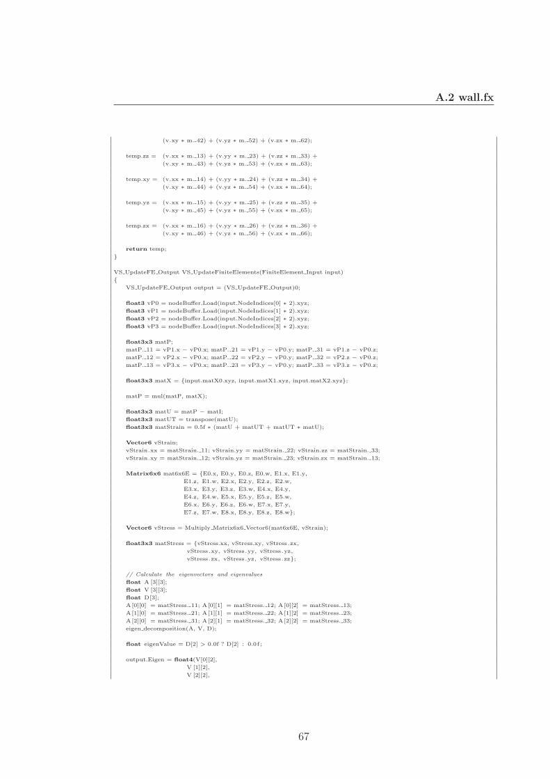
A.2 wall.fx

(v.xy ∗ m. 42) + (v.yz ∗ m. 52) + (v.zx ∗ m. 62);

temp.zz = (v.xx ∗ m. 13) + (v.yy ∗ m. 23) + (v.zz ∗ m. 33) +

(v.xy ∗ m. 43) + (v.yz ∗ m. 53) + (v.zx ∗ m. 63);

temp.xy = (v.xx ∗ m. 14) + (v.yy ∗ m. 24) + (v.zz ∗ m. 34) +

(v.xy ∗ m. 44) + (v.yz ∗ m. 54) + (v.zx ∗ m. 64);

temp.yz = (v.xx ∗ m. 15) + (v.yy ∗ m. 25) + (v.zz ∗ m. 35) +

(v.xy ∗ m. 45) + (v.yz ∗ m. 55) + (v.zx ∗ m. 65);

temp.zx = (v.xx ∗ m. 16) + (v.yy ∗ m. 26) + (v.zz ∗ m. 36) +

(v.xy ∗ m. 46) + (v.yz ∗ m. 56) + (v.zx ∗ m. 66);

return temp;

}

VS UpdateFE Output VS UpdateFiniteElements(FiniteElement Input input)

{

VS UpdateFE Output output = (VS UpdateFE Output)0;

float3 vP0 = nodeBuffer.Load(input.NodeIndices[0] ∗ 2).xyz;

float3 vP1 = nodeBuffer.Load(input.NodeIndices[1] ∗ 2).xyz;

float3 vP2 = nodeBuffer.Load(input.NodeIndices[2] ∗ 2).xyz;

float3 vP3 = nodeBuffer.Load(input.NodeIndices[3] ∗ 2).xyz;

float3x3 matP;

matP. 11 = vP1.x − vP0.x; matP. 21 = vP1.y − vP0.y; matP. 31 = vP1.z − vP0.z;

matP. 12 = vP2.x − vP0.x; matP. 22 = vP2.y − vP0.y; matP. 32 = vP2.z − vP0.z;

matP. 13 = vP3.x − vP0.x; matP. 23 = vP3.y − vP0.y; matP. 33 = vP3.z − vP0.z;

float3x3 matX = {input.matX0.xyz, input.matX1.xyz, input.matX2.xyz};

matP = mul(matP, matX);

float3x3 matU = matP − matI;

float3x3 matUT = transpose(matU);

float3x3 matStrain = 0.5f ∗ (matU + matUT + matUT ∗ matU);

Vector6 vStrain;

vStrain.xx = matStrain. 11; vStrain.yy = matStrain. 22; vStrain.zz = matStrain. 33;

vStrain.xy = matStrain. 12; vStrain.yz = matStrain. 23; vStrain.zx = matStrain. 13;

Matrix6x6 mat6x6E = {E0.x, E0.y, E0.z, E0.w, E1.x, E1.y,

E1.z, E1.w, E2.x, E2.y, E2.z, E2.w,

E3.x, E3.y, E3.z, E3.w, E4.x, E4.y,

E4.z, E4.w, E5.x, E5.y, E5.z, E5.w,

E6.x, E6.y, E6.z, E6.w, E7.x, E7.y,

E7.z, E7.w, E8.x, E8.y, E8.z, E8.w};

Vector6 vStress = Multiply Matrix6x6 Vector6(mat6x6E, vStrain);

float3x3 matStress = {vStress.xx, vStress.xy, vStress.zx,

vStress.xy, vStress.yy, vStress.yz,

vStress.zx, vStress.yz, vStress.zz};

// Calculate the eigenvectors and eigenvalues

float A [3][3];

float V [3][3];

float D[3];

A [0][0] = matStress. 11; A[0][1] = matStress. 12; A[0][2] = matStress. 13;

A [1][0] = matStress. 21; A[1][1] = matStress. 22; A[1][2] = matStress. 23;

A [2][0] = matStress. 31; A[2][1] = matStress. 32; A[2][2] = matStress. 33;

eigen decomposition(A, V, D);

float eigenValue = D[2] > 0.0f ? D[2] : 0.0f ;

output.Eigen = float4(V[0][2],

V [1][2],

V [2][2],

67

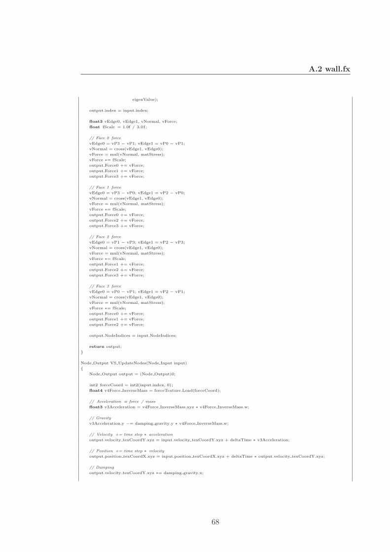
A.2 wall.fx

eigenValue);

output.index = input.index;

float3 vEdge0, vEdge1, vNormal, vForce;

float fScale = 1.0f / 3.0f ;

// Face 0 force

vEdge0 = vP3 − vP1; vEdge1 = vP0 − vP1;

vNormal = cross(vEdge1, vEdge0);

vForce = mul(vNormal, matStress);

vForce ∗= fScale;

output.Force0 += vForce;

output.Force1 += vForce;

output.Force3 += vForce;

// Face 1 force

vEdge0 = vP3 − vP0; vEdge1 = vP2 − vP0;

vNormal = cross(vEdge1, vEdge0);

vForce = mul(vNormal, matStress);

vForce ∗= fScale;

output.Force0 += vForce;

output.Force2 += vForce;

output.Force3 += vForce;

// Face 2 force

vEdge0 = vP1 − vP3; vEdge1 = vP2 − vP3;

vNormal = cross(vEdge1, vEdge0);

vForce = mul(vNormal, matStress);

vForce ∗= fScale;

output.Force1 += vForce;

output.Force2 += vForce;

output.Force3 += vForce;

// Face 3 force

vEdge0 = vP0 − vP1; vEdge1 = vP2 − vP1;

vNormal = cross(vEdge1, vEdge0);

vForce = mul(vNormal, matStress);

vForce ∗= fScale;

output.Force0 += vForce;

output.Force1 += vForce;

output.Force2 += vForce;

output.NodeIndices = input.NodeIndices;

return output;

}

Node Output VS UpdateNodes(Node Input input)

{

Node Output output = (Node Output)0;

int2 forceCoord = int2(input.index, 0);

float4 v4Force InverseMass = forceTexture.Load(forceCoord);

// Acceleration = force / mass

float3 v3Acceleration = v4Force InverseMass.xyz ∗ v4Force InverseMass.w;

// Gravity

v3Acceleration.y −= damping gravity.y ∗ v4Force InverseMass.w;

// Velocity += time step ∗ acceleration

output.velocity texCoordY.xyz = input.velocity texCoordY.xyz + deltaTime ∗ v3Acceleration;

// Position += time step ∗ velocity

output.position texCoordX.xyz = input.position texCoordX.xyz + deltaTime ∗ output.velocity texCoordY.xyz;

// Damping

output.velocity texCoordY.xyz ∗= damping gravity.x;

68

A.2 wall.fx

// Copy over tex coords − only need to do this if not skipping data fields with the GS Output

output.position texCoordX.w = input.position texCoordX.w;

output.velocity texCoordY.w = input.velocity texCoordY.w;

return output;

}

FiniteElement Output VS UpdateFracture(FiniteElement Input input)

{

FiniteElement Output output = (FiniteElement Output)0;

int2 eigenCoord = int2(input.index, 0);

float4 v4Eigen = eigenTexture.Load(eigenCoord);

output.NodeIndices = input.NodeIndices;

output.matX0 = input.matX0;

output.matX1 = input.matX1;

output.matX2 = input.matX2;

return output;

}

FiniteElement Output VS DrawSim(FiniteElement Input input)

{

FiniteElement Output output = (FiniteElement Output)0;

output.NodeIndices = input.NodeIndices;

output.matX0 = input.matX0;

output.matX1 = input.matX1;

output.matX2 = input.matX2;

return output;

}

VS DrawDisplay Output VS DrawDisplay(VS DrawDisplay Input input)

{

VS DrawDisplay Output output = (VS DrawDisplay Output)0;

output.Position = input.Position;

output.TexCoord = input.TexCoord;

return output;

}

// Geometry Shaders

//=================

[maxvertexcount(5)]

void GS UpdateFiniteElements(point VS UpdateFE Output input[1], inout PointStream<GS UpdateFE Output> pointStream

)

{

GS UpdateFE Output output = (GS UpdateFE Output)0;

// won’t compile with an array of 4 elements for some reason !!!!!

//float3 forces [4] = {input [0].Force0, input [0]. Force1, input [0]. Force2, input [0]. Force3};

float3 forces [5];

forces [0] = input[0].Force0;

forces [1] = input[0].Force1;

forces [2] = input[0].Force2;

forces [3] = input[0].Force3;

uint index;

output.Position.yz = 0.0f;

output.Position.w = 1.0f;

// Output the 4 forces for the 1st render target

for(int i = 0; i < 4; i++)

{

69

A.2 wall.fx

index = input[0].NodeIndices[i ];

output.Position.x = −1.0f + textureIncrement + (index ∗ textureIncrement);

output.CombinedForce = forces[i];

output.Eigen.xyzw = 0.0f;

pointStream.Append(output);

}

// Output the eigen vector and value for the 2nd render target

output.Position.x = −1.0f + textureIncrement + (input[0].index ∗ textureIncrement);

output.CombinedForce.xyz = 0.0f;

output.Eigen = input[0].Eigen;

pointStream.Append(output);

}

[maxvertexcount(12)]

void GS DrawSim(point FiniteElement Output input[1], inout TriangleStream<GS DrawSim Output> TriStream)

{

GS DrawSim Output output = (GS DrawSim Output)0;

float4 vPWorld[4] = {{0,0,0,0},{0,0,0,0},{0,0,0,0},{0,0,0,0}};

float4 vP[4] = {{0,0,0,0},{0,0,0,0},{0,0,0,0},{0,0,0,0}};

float2 vT[4] = {{0,0},{0,0},{0,0},{0,0}};

for (int i = 0; i < 4; i++)

{

float4 position texCoordX = nodeBuffer.Load(input[0].NodeIndices[i] ∗ 2);

float4 velocity texCoordY = nodeBuffer.Load(input[0].NodeIndices[i] ∗ 2 + 1);

vPWorld[i] = float4(position texCoordX.xyz, 1.0f);

vP[i] = mul(vPWorld[i], worldViewProjection);

vT[i ]. x = position texCoordX.w;

vT[i ]. y = velocity texCoordY.w;

}

int3 faceIndices [4] = {int3(1,3,0) , int3 (0,3,2) , int3 (3,1,2) , int3 (1,0,2) };

float3 faceEdgeA = float3(0,0,0);

float3 faceEdgeB = float3(0,0,0);

float3 faceNormal = float3(0,0,0);

float dirlight = 0.0f;

float light = 0.0f;

for (int j = 0; j < 4; j++) // for each face

{

faceEdgeA = vPWorld[faceIndices[j][1]].xyz − vPWorld[faceIndices[j ][0]]. xyz;

faceEdgeB = vPWorld[faceIndices[j][2]].xyz − vPWorld[faceIndices[j ][0]]. xyz;

faceNormal = normalize(cross(faceEdgeA, faceEdgeB));

dirlight = 0.75f ∗ saturate(dot (faceNormal, −normalize(lightDirection)));

light = 0.25f + dirlight ;

output.Color = float3(light, light , light ) ;

output.Position = vP[faceIndices[j ][0]];

output.TexCoord = vT[faceIndices[j ][0]];

TriStream.Append( output );

output.Position = vP[faceIndices[j ][1]];

output.TexCoord = vT[faceIndices[j ][1]];

TriStream.Append( output );

output.Position = vP[faceIndices[j ][2]];

output.TexCoord = vT[faceIndices[j ][2]];

TriStream.Append( output );

TriStream.RestartStrip();

}

}

[maxvertexcount(3)]

void GS DrawDisplay(triangle VS DrawDisplay Output input[3], inout TriangleStream<GS DrawDisplay Output> TriStream)

{

GS DrawDisplay Output output = (GS DrawDisplay Output)0;

70

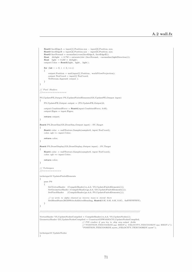
A.2 wall.fx

float3 faceEdgeA = input[1].Position.xyz − input[0].Position.xyz;

float3 faceEdgeB = input[2].Position.xyz − input[0].Position.xyz;

float3 faceNormal = normalize(cross(faceEdgeA, faceEdgeB));

float dirlight = 0.75f ∗ saturate(dot (faceNormal, −normalize(lightDirection)));

float light = 0.25f + dirlight ;

output.Color = float3(light, light , light ) ;

for (int i = 0; i < 3; i++)

{

output.Position = mul(input[i].Position, worldViewProjection);

output.TexCoord = input[i].TexCoord;

TriStream.Append( output );

}

}

// Pixel Shaders

//==============

PS UpdateFE Output PS UpdateFiniteElements(GS UpdateFE Output input)

{

PS UpdateFE Output output = (PS UpdateFE Output)0;

output.CombinedForce = float4(input.CombinedForce, 0.0f);

output.Eigen = input.Eigen;

return output;

}

float4 PS DrawSim(GS DrawSim Output input) : SV Target

{

float4 color = wallTexture.Sample(sampler0, input.TexCoord);

color .rgb ∗= input.Color;

return color;

}

float4 PS DrawDisplay(GS DrawDisplay Output input) : SV Target

{

float4 color = wallTexture.Sample(sampler0, input.TexCoord);

color .rgb ∗= input.Color;

return color;

}

// Techniques

//===========

technique10 UpdateFiniteElements

{

pass P0

{

SetVertexShader (CompileShader(vs 4 0, VS UpdateFiniteElements()));

SetGeometryShader (CompileShader(gs 4 0, GS UpdateFiniteElements()));

SetPixelShader (CompileShader(ps 4 0, PS UpdateFiniteElements()));

// no write to alpha channel as inverse mass is stored there

SetBlendState(RGBWriteAdditiveBlending, float4(0.0f, 0.0f, 0.0f, 0.0f) , 0xFFFFFFFF);

}

}

//////////////////////////////////////////////////////////////////////////////////////

VertexShader VS UpdateNodesCompiled = CompileShader(vs 4 0, VS UpdateNodes());

GeometryShader GS UpdateNodesCompiled = ConstructGSWithSO(VS UpdateNodesCompiled,

// PIX crashes if you try to skip any output fields

//”POSITION TEXCOORDX.xyz; $SKIP.x; VELOCITY TEXCOORDY.xyz; $SKIP.x”);

”POSITION TEXCOORDX.xyzw; VELOCITY TEXCOORDY.xyzw”);

technique10 UpdateNodes

{

71

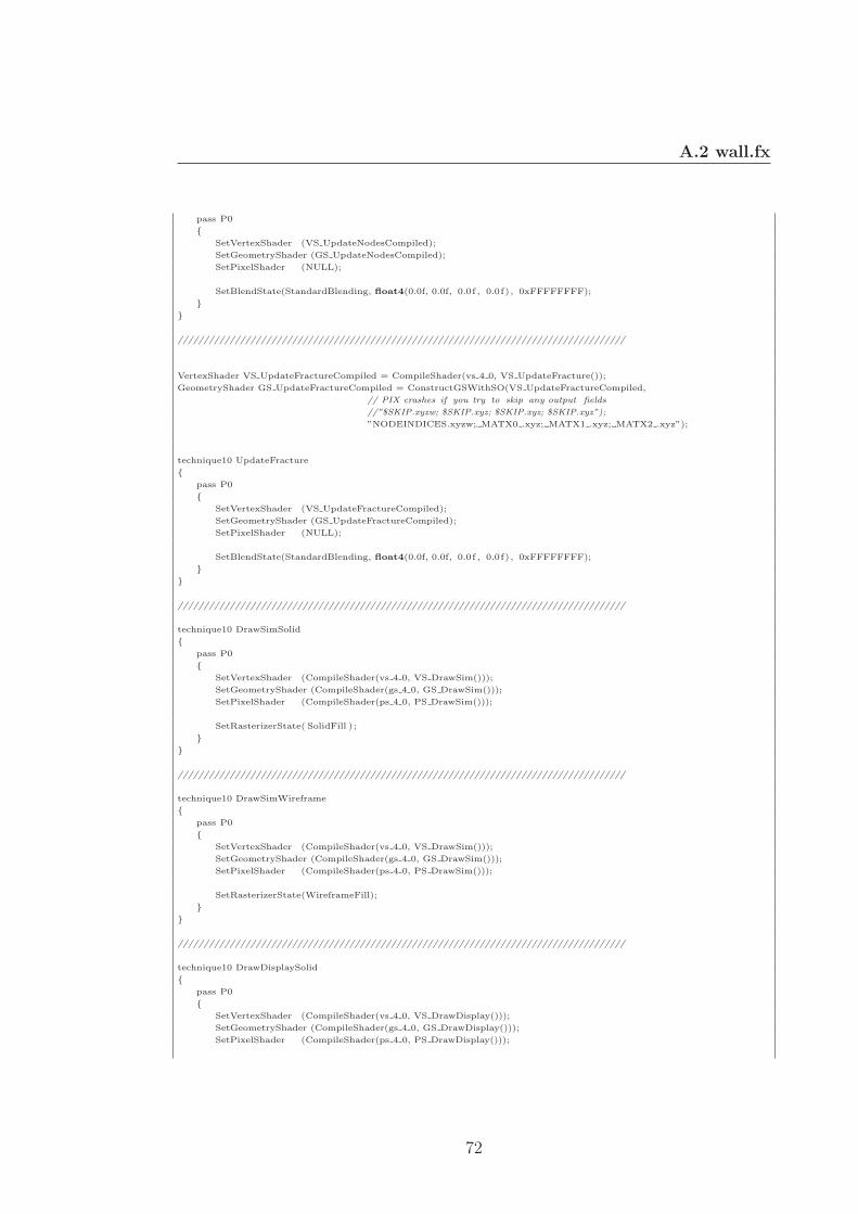
A.2 wall.fx

pass P0

{

SetVertexShader (VS UpdateNodesCompiled);

SetGeometryShader (GS UpdateNodesCompiled);

SetPixelShader (NULL);

SetBlendState(StandardBlending, float4(0.0f, 0.0f, 0.0f , 0.0f) , 0xFFFFFFFF);

}

}

//////////////////////////////////////////////////////////////////////////////////////

VertexShader VS UpdateFractureCompiled = CompileShader(vs 4 0, VS UpdateFracture());

GeometryShader GS UpdateFractureCompiled = ConstructGSWithSO(VS UpdateFractureCompiled,

// PIX crashes if you try to skip any output fields

//”$SKIP.xyzw; $SKIP.xyz; $SKIP.xyz; $SKIP.xyz”);

”NODEINDICES.xyzw; MATX0 .xyz; MATX1 .xyz; MATX2 .xyz”);

technique10 UpdateFracture

{

pass P0

{

SetVertexShader (VS UpdateFractureCompiled);

SetGeometryShader (GS UpdateFractureCompiled);

SetPixelShader (NULL);

SetBlendState(StandardBlending, float4(0.0f, 0.0f, 0.0f , 0.0f) , 0xFFFFFFFF);

}

}

//////////////////////////////////////////////////////////////////////////////////////

technique10 DrawSimSolid

{

pass P0

{

SetVertexShader (CompileShader(vs 4 0, VS DrawSim()));

SetGeometryShader (CompileShader(gs 4 0, GS DrawSim()));

SetPixelShader (CompileShader(ps 4 0, PS DrawSim()));

SetRasterizerState( SolidFill ) ;

}

}

//////////////////////////////////////////////////////////////////////////////////////

technique10 DrawSimWireframe

{

pass P0

{

SetVertexShader (CompileShader(vs 4 0, VS DrawSim()));

SetGeometryShader (CompileShader(gs 4 0, GS DrawSim()));

SetPixelShader (CompileShader(ps 4 0, PS DrawSim()));

SetRasterizerState(WireframeFill);

}

}

//////////////////////////////////////////////////////////////////////////////////////

technique10 DrawDisplaySolid

{

pass P0

{

SetVertexShader (CompileShader(vs 4 0, VS DrawDisplay()));

SetGeometryShader (CompileShader(gs 4 0, GS DrawDisplay()));

SetPixelShader (CompileShader(ps 4 0, PS DrawDisplay()));

72

A.2 wall.fx

SetRasterizerState( SolidFill ) ;

}

}

//////////////////////////////////////////////////////////////////////////////////////

technique10 DrawDisplayWireframe

{

pass P0

{

SetVertexShader (CompileShader(vs 4 0, VS DrawDisplay()));

SetGeometryShader (CompileShader(gs 4 0, GS DrawDisplay()));

SetPixelShader (CompileShader(ps 4 0, PS DrawDisplay()));

SetRasterizerState(WireframeFill);

}

}

73

REFERENCES

References

Akenine-Moller, T., Haines, E. and Hoffman, N. 2008. Real-Time

Rendering 3rd Edition. A. K. Peters, Ltd, Natick, MA, USA.

Barnes, C. 2007. Eigenvectors of 3x3 symmetric matrix.

http://barnesc.blogspot.com/2007/02/eigenvectors-of-3x3-symmetric-

matrix.html.

Buck, I., Foley, T., Horn, D., Sugerman, J., Fatahalian, K., Hous-

ton, M. and Hanrahan, P. 2004. Brook for gpus: Stream computing on

graphics hardware. ACM TRANSACTIONS ON GRAPHICS 23 , pp. 777–786.

Gummaraju, J. and Rosenblum, M. 2005. Stream programming on general-

purpose processors. In MICRO 38: Proceedings of the 38th annual IEEE/ACM

International Symposium on Microarchitecture, IEEE Computer Society, Wash-

ington, DC, USA, pp. 343–354.

Khronos. 2010a. Opencl. Available on-line at http://www.khronos.org/opencl/.

Khronos. 2010b. Opengl shading language. Available on-line at

http://www.opengl.org/documentation/glsl/.

LucasArts. 2008. Star wars : the force unleashed. Available on-line at

http://www.lucasarts.com/games/theforceunleashed.

MacDonald, B. J. 2007. Practical Stress Analysis with Finite Elements. Glas-

nevin Publishing, Ireland.

MSDN. 2010a. Dxut programming guide. Available on-line at

http://msdn.microsoft.com/en-us/library/ee417532(v=VS.85).aspx.

MSDN. 2010b. Hlsl (windows). Available on-line at

http://msdn.microsoft.com/en-us/library/bb509561(v=vs.85).aspx.

MSDN. 2010c. Multiple render targets (direct3d

10). Available on-line at http://msdn.microsoft.com/en-

us/library/bb205131(VS.85).aspx#Multiple Rendertargets.

74

REFERENCES

MSDN. 2010d. Pipeline stages (direct3d 10). Available on-line at

http://msdn.microsoft.com/en-us/library/bb205123(VS.85).aspx.

MSDN. 2010e. Semantics (directx hlsl). Available on-line at

http://msdn.microsoft.com/en-us/library/bb509647(VS.85).aspx.

MSDN. 2010f. Stream out syntax. Available on-line at

http://msdn.microsoft.com/en-us/library/ff476168(VS.85).aspx.

MSDN. 2010g. Stream-output stage (direct3d 10) (windows). Available on-line

at http://msdn.microsoft.com/en-us/library/bb205121(VS.85).aspx.

Muller, M., McMillan, L., Dorsey, J. and Jagnow, R. 2001. Real-time

simulation of deformation and fracture of stiff materials. In Proceedings of the

Eurographic workshop on Computer animation and simulation, Springer-Verlag

New York, Inc, New York, NY, USA, pp. 113–124.

Muller, M., Stam, J., James, D. and Thurey, N. 2008. Real time physics:

class notes. In SIGGRAPH ’08: ACM SIGGRAPH 2008 classes, ACM, New

York, NY, USA, pp. 1–90.

NVIDIA. 2008. Gpu programming guide geforce 8 and 9 series. Available on-line

at http://developer.nvidia.com/object/gpu programming guide.html.

NVIDIA. 2010a. Cg - the language for high-performance realtime graphics.

Available on-line at http://developer.nvidia.com/page/cg main.html.

NVIDIA. 2010b. Directcompute. Available on-line at

http://www.nvidia.com/object/cuda directcompute.html.

NVIDIA. 2010c. Physx. Available on-line at

http://www.nvidia.com/object/physx new.html.

NVIDIA. 2011. Cuda. Available on-line at

http://developer.nvidia.com/category/zone/cuda-zone.

75

REFERENCES

O’Brien, J. F. and Hodgins, J. K. 1999. Graphical modeling and animation

of brittle fracture. In SIGGRAPH ’99: Proceedings of the 26th annual confer-

ence on Computer graphics and interactive techniques, ACM Press/Addison-

Wesley Publishing Co, New York, NY, USA, pp. 137–146.

O’Brien, J. F., Bargteil, A. W. and Hodgins, J. K. 2002. Graphical

modeling and animation of ductile fracture. In SIGGRAPH ’02: Proceedings of

the 29th annual conference on Computer graphics and interactive techniques,

ACM, New York, NY, USA, pp. 291–294.

O’Sullivan, C., Dingliana, J., Giang, T. and Kaiser, M. K. 2003. Eval-

uating the visual fidelity of physically based animations. In ACM SIGGRAPH

2003 Papers, ACM, New York, NY, USA, SIGGRAPH ’03, pp. 527–536.

Parker, E. G. and O’Brien, J. F. 2009. Real-time deformation and fracture

in a game environment. In SCA ’09: Proceedings of the 2009 ACM SIG-

GRAPH/Eurographics Symposium on Computer Animation, ACM, New York,

NY, USA, pp. 165–175.

Pixelux. 2010. Digital molecular matter. Available on-line at

http://www.pixelux.com.

Scheepers, F. and Whittock, A. 2006. The wrecked road in cars - or how

to damage perfectly good geometry. p. 97.

Terzopoulos, D., Platt, J., Barr, A. and Fleischer, K. 1987. Elasti-

cally deformable models. In SIGGRAPH ’87: Proceedings of the 14th annual

conference on Computer graphics and interactive techniques, ACM, New York,

NY, USA, pp. 205–214.

76