GPL Reference Guide for IBM SPSS Statistics line in the example is a statement.One or more statements make up a block of GPL. Each statement specifies an aspect of the graph, such

GPL Reference Guide for IBM SPSSStatistics

��

NoteBefore using this information and the product it supports, read the information in “Notices” on page 415.

Product Information

This edition applies to version 162261647161, release 0, modification 0 of IBM SPSS Modeler BatchIBM SPSSModelerIBM SPSS Modeler ServerIBM SPSS StatisticsIBM SPSS Statistics ServerIBM SPSS AmosIBM SPSSSmartreaderIBM SPSS Statistics Base Integrated Student EditionIBM SPSS Collaboration and DeploymentServicesIBM SPSS Visualization DesignerIBM SPSS Modeler Text AnalyticsIBM SPSS Text Analytics for Surveys IBMAnalytical Decision ManagementIBM SPSS Modeler Social Network AnalysisIBM SPSS Analytic Server and to allsubsequent releases and modifications until otherwise indicated in new editions.

Contents

Chapter 1. Introduction to GPL . . . . . 1The Basics . . . . . . . . . . . . . . . 1GPL Syntax Rules. . . . . . . . . . . . . 3GPL Concepts . . . . . . . . . . . . . . 3

Brief Overview of GPL Algebra . . . . . . . 3How Coordinates and the GPL Algebra Interact . 6

Common Tasks . . . . . . . . . . . . . 14How to Add Stacking to a Graph . . . . . . 14How to Add Faceting (Paneling) to a Graph . . 15How to Add Clustering to a Graph . . . . . 17How to Use Aesthetics . . . . . . . . . 18

Chapter 2. GPL Statement andFunction Reference . . . . . . . . . 21GPL Statements . . . . . . . . . . . . . 21

COMMENT Statement. . . . . . . . . . 21PAGE Statement . . . . . . . . . . . . 22GRAPH Statement . . . . . . . . . . . 22SOURCE Statement. . . . . . . . . . . 23DATA Statement. . . . . . . . . . . . 24TRANS Statement . . . . . . . . . . . 24COORD Statement . . . . . . . . . . . 25SCALE Statement . . . . . . . . . . . 29GUIDE Statement . . . . . . . . . . . 41ELEMENT Statement . . . . . . . . . . 46

GPL Functions . . . . . . . . . . . . . 56aestheticMaximum Function . . . . . . . . 63aestheticMinimum Function . . . . . . . . 64aestheticMissing Function . . . . . . . . 65alpha Function . . . . . . . . . . . . 65base Function. . . . . . . . . . . . . 66base.aesthetic Function . . . . . . . . . 66base.all Function. . . . . . . . . . . . 67base.coordinate Function . . . . . . . . . 68begin Function (For GPL Graphs) . . . . . . 69begin Function (For GPL Pages) . . . . . . 69beta Function . . . . . . . . . . . . . 69bin.dot Function . . . . . . . . . . . . 70bin.hex Function. . . . . . . . . . . . 72bin.quantile.letter Function . . . . . . . . 75bin.rect Function. . . . . . . . . . . . 77binCount Function . . . . . . . . . . . 79binStart Function . . . . . . . . . . . 80binWidth Function . . . . . . . . . . . 81chiSquare Function . . . . . . . . . . . 81closed Function . . . . . . . . . . . . 81cluster Function . . . . . . . . . . . . 82col Function . . . . . . . . . . . . . 84collapse Function . . . . . . . . . . . 85color Function (For GPL Graphic Elements). . . 86color Function (For GPL Guides) . . . . . . 87color.brightness Function (For GPL GraphicElements) . . . . . . . . . . . . . . 88color.brightness Function (For GPL Guides). . . 88color.hue Function (For GPL Graphic Elements) 89

color.hue Function (For GPL Guides) . . . . . 90color.saturation Function (For GPL GraphicElements) . . . . . . . . . . . . . . 90color.saturation Function (For GPL Guides) . . . 91csvSource Function . . . . . . . . . . . 92dataMaximum Function . . . . . . . . . 92dataMinimum Function . . . . . . . . . 93delta Function . . . . . . . . . . . . 93density.beta Function . . . . . . . . . . 93density.chiSquare Function . . . . . . . . 96density.exponential Function. . . . . . . . 98density.f Function . . . . . . . . . . . 100density.gamma Function. . . . . . . . . 102density.kernel Function . . . . . . . . . 105density.logistic Function . . . . . . . . . 108density.normal Function . . . . . . . . . 110density.poisson Function. . . . . . . . . 112density.studentizedRange Function . . . . . 115density.t Function . . . . . . . . . . . 117density.uniform Function . . . . . . . . 119density.weibull Function. . . . . . . . . 121dim Function . . . . . . . . . . . . 124end Function . . . . . . . . . . . . 125eval Function . . . . . . . . . . . . 126exclude Function . . . . . . . . . . . 130exponent Function. . . . . . . . . . . 130exponential Function . . . . . . . . . . 131f Function . . . . . . . . . . . . . 131format Function . . . . . . . . . . . 131format.date Function . . . . . . . . . . 132format.dateTime Function . . . . . . . . 132format.time Function . . . . . . . . . . 133from Function . . . . . . . . . . . . 133gamma Function . . . . . . . . . . . 133gap Function . . . . . . . . . . . . 134gridlines Function . . . . . . . . . . . 134in Function . . . . . . . . . . . . . 135include Function . . . . . . . . . . . 135index Function . . . . . . . . . . . . 136iter Function . . . . . . . . . . . . 136jump Function . . . . . . . . . . . . 136label Function (For GPL Graphic Elements) . . 137label Function (For GPL Guides) . . . . . . 138layout.circle Function. . . . . . . . . . 139layout.dag Function . . . . . . . . . . 141layout.data Function . . . . . . . . . . 143layout.grid Function . . . . . . . . . . 145layout.network Function. . . . . . . . . 147layout.random Function . . . . . . . . . 150layout.tree Function . . . . . . . . . . 152link.alpha Function . . . . . . . . . . 154link.complete Function . . . . . . . . . 156link.delaunay Function . . . . . . . . . 159link.distance Function . . . . . . . . . 161link.gabriel Function . . . . . . . . . . 163link.hull Function . . . . . . . . . . . 165

iii

link.influence Function . . . . . . . . . 168link.join Function . . . . . . . . . . . 170link.mst Function . . . . . . . . . . . 172link.neighbor Function . . . . . . . . . 175link.relativeNeighborhood Function . . . . . 177link.sequence Function . . . . . . . . . 179link.tsp Function . . . . . . . . . . . 181logistic Function . . . . . . . . . . . 183map Function . . . . . . . . . . . . 184marron Function . . . . . . . . . . . 184max Function . . . . . . . . . . . . 185min Function . . . . . . . . . . . . 185mirror Function . . . . . . . . . . . 186missing.gap Function . . . . . . . . . . 186missing.interpolate Function . . . . . . . 187missing.listwise Function . . . . . . . . 187missing.pairwise Function . . . . . . . . 188missing.wings Function . . . . . . . . . 188multiple Function . . . . . . . . . . . 188noConstant Function . . . . . . . . . . 189node Function . . . . . . . . . . . . 189notIn Function . . . . . . . . . . . . 190normal Function . . . . . . . . . . . 190opposite Function . . . . . . . . . . . 190origin Function (For GPL Graphs) . . . . . 191origin Function (For GPL Scales) . . . . . . 191poisson Function . . . . . . . . . . . 192position Function (For GPL Graphic Elements) 192position Function (For GPL Guides) . . . . . 193preserveStraightLines Function . . . . . . 194project Function . . . . . . . . . . . 194proportion Function . . . . . . . . . . 195reflect Function. . . . . . . . . . . . 195region.confi.count Function . . . . . . . . 196region.confi.mean Function . . . . . . . . 198region.confi.percent.count Function . . . . . 200region.confi.proportion.count Function . . . . 202region.confi.smooth Function . . . . . . . 205region.spread.range Function . . . . . . . 207region.spread.sd Function . . . . . . . . 209region.spread.se Function . . . . . . . . 212reverse Function . . . . . . . . . . . 214root Function . . . . . . . . . . . . 215sameRatio Function . . . . . . . . . . 215savSource Function . . . . . . . . . . 216scale Function (For GPL Axes). . . . . . . 216scale Function (For GPL Graphs) . . . . . . 217scale Function (For GPL Graphic Elements andform.line). . . . . . . . . . . . . . 217scale Function (For GPL Pages) . . . . . . 218scaledToData Function . . . . . . . . . 218segments Function. . . . . . . . . . . 219shape Function (For GPL Graphic Elements) . . 219shape Function (For GPL Guides) . . . . . 220showAll Function . . . . . . . . . . . 221size Function (For GPL Graphic Elements). . . 221size Function (For GPL Guides) . . . . . . 222smooth.cubic Function . . . . . . . . . 222smooth.linear Function . . . . . . . . . 225smooth.loess Function . . . . . . . . . 227smooth.mean Function . . . . . . . . . 230

smooth.median Function . . . . . . . . 232smooth.quadratic Function . . . . . . . . 235smooth.spline Function . . . . . . . . . 237smooth.step Function. . . . . . . . . . 239sort.data Function . . . . . . . . . . . 241sort.natural Function . . . . . . . . . . 241sort.statistic Function . . . . . . . . . . 242sort.values Function . . . . . . . . . . 242split Function . . . . . . . . . . . . 243sqlSource Function . . . . . . . . . . 243start Function . . . . . . . . . . . . 244startAngle Function . . . . . . . . . . 244studentizedRange Function . . . . . . . . 245summary.count Function . . . . . . . . 245summary.count.cumulative Function. . . . . 247summary.countTrue Function . . . . . . . 250summary.first Function . . . . . . . . . 252summary.kurtosis Function . . . . . . . . 254summary.last Function . . . . . . . . . 257summary.max Function . . . . . . . . . 259summary.mean Function . . . . . . . . 261summary.median Function . . . . . . . . 263summary.min Function . . . . . . . . . 265summary.mode Function . . . . . . . . 268summary.percent Function . . . . . . . . 270summary.percent.count Function . . . . . . 271summary.percent.count.cumulative Function . . 274summary.percent.cumulative Function . . . . 276summary.percent.sum Function . . . . . . 278summary.percent.sum.cumulative Function . . 281summary.percentile Function . . . . . . . 283summary.percentTrue Function . . . . . . 285summary.proportion Function . . . . . . . 288summary.proportion.count Function . . . . . 289summary.proportion.count.cumulative Function 292summary.proportion.cumulative Function . . . 294summary.proportion.sum Function . . . . . 294summary.proportion.sum.cumulative Function 297summary.proportionTrue Function . . . . . 299summary.range Function . . . . . . . . 302summary.sd Function. . . . . . . . . . 304summary.se Function . . . . . . . . . . 306summary.se.kurtosis Function . . . . . . . 308summary.se.skewness Function . . . . . . 311summary.sum Function . . . . . . . . . 313summary.sum.cumulative Function . . . . . 315summary.variance Function. . . . . . . . 317t Function . . . . . . . . . . . . . 320texture.pattern Function . . . . . . . . . 320ticks Function . . . . . . . . . . . . 321to Function . . . . . . . . . . . . . 321transparency Function (For GPL GraphicElements). . . . . . . . . . . . . . 322transparency Function (For GPL Guides) . . . 323transpose Function . . . . . . . . . . 323uniform Function . . . . . . . . . . . 324unit.percent Function . . . . . . . . . . 324userSource Function . . . . . . . . . . 324values Function . . . . . . . . . . . 325visible Function . . . . . . . . . . . 325weibull Function . . . . . . . . . . . 326

iv GPL Reference Guide for IBM SPSS Statistics

weight Function . . . . . . . . . . . 326wrap Function . . . . . . . . . . . . 327

Chapter 3. GPL Examples . . . . . . 329Using the Examples in Your Application . . . . 329Summary Bar Chart Examples. . . . . . . . 330

Simple Bar Chart . . . . . . . . . . . 330Simple Bar Chart of Counts . . . . . . . 331Simple Horizontal Bar Chart . . . . . . . 332Simple Bar Chart With Error Bars . . . . . 333Simple Bar Chart with Bar for All Categories 334Stacked Bar Chart . . . . . . . . . . . 335Clustered Bar Chart . . . . . . . . . . 336Clustered and Stacked Bar Chart . . . . . . 339Bar Chart Using an Evaluation Function . . . 340Bar Chart with Mapped Aesthetics . . . . . 341Faceted (Paneled) Bar Chart . . . . . . . 3423-D Bar Chart . . . . . . . . . . . . 346Error Bar Chart. . . . . . . . . . . . 347

Histogram Examples . . . . . . . . . . . 347Histogram . . . . . . . . . . . . . 348Histogram with Distribution Curve . . . . . 349Percentage Histogram . . . . . . . . . 351Frequency Polygon . . . . . . . . . . 352Stacked Histogram . . . . . . . . . . 353Faceted (Paneled) Histogram . . . . . . . 354Population Pyramid . . . . . . . . . . 355Cumulative Histogram . . . . . . . . . 3563-D Histogram . . . . . . . . . . . . 357

High-Low Chart Examples . . . . . . . . . 357Simple Range Bar for One Variable . . . . . 358Simple Range Bar for Two Variables . . . . . 359High-Low-Close Chart . . . . . . . . . 360

Scatter/Dot Examples . . . . . . . . . . 361Simple 1-D Scatterplot . . . . . . . . . 361Simple 2-D Scatterplot . . . . . . . . . 362Simple 2-D Scatterplot with Fit Line . . . . . 363Grouped Scatterplot . . . . . . . . . . 364Grouped Scatterplot with Convex Hull . . . . 365Scatterplot Matrix (SPLOM) . . . . . . . 366Bubble Plot . . . . . . . . . . . . . 367Binned Scatterplot . . . . . . . . . . . 368Binned Scatterplot with Polygons. . . . . . 369Scatterplot with Border Histograms . . . . . 370Scatterplot with Border Boxplots . . . . . . 371Dot Plot . . . . . . . . . . . . . . 372

2-D Dot Plot. . . . . . . . . . . . . 374Jittered Categorical Scatterplot. . . . . . . 376

Line Chart Examples . . . . . . . . . . . 377Simple Line Chart . . . . . . . . . . . 377Simple Line Chart with Points. . . . . . . 378Line Chart of Date Data . . . . . . . . . 379Line Chart With Step Interpolation . . . . . 380Fit Line . . . . . . . . . . . . . . 381Line Chart from Equation . . . . . . . . 382Line Chart with Separate Scales . . . . . . 384

Pie Chart Examples . . . . . . . . . . . 385Pie Chart . . . . . . . . . . . . . . 385Paneled Pie Chart . . . . . . . . . . . 387Stacked Pie Chart . . . . . . . . . . . 388

Boxplot Examples . . . . . . . . . . . . 3891-D Boxplot . . . . . . . . . . . . . 389Boxplot . . . . . . . . . . . . . . 390Clustered Boxplot . . . . . . . . . . . 392Boxplot With Overlaid Dot Plot . . . . . . 393

Multi-Graph Examples . . . . . . . . . . 394Scatterplot with Border Histograms . . . . . 395Scatterplot with Border Boxplots . . . . . . 397Stocks Line Chart with Volume Bar Chart . . . 399Dual Axis Graph . . . . . . . . . . . 400Histogram with Dot Plot . . . . . . . . 402

Other Examples . . . . . . . . . . . . 403Collapsing Small Categories . . . . . . . 403Mapping Aesthetics . . . . . . . . . . 405Faceting by Separate Variables. . . . . . . 406Grouping by Separate Variables . . . . . . 406Clustering Separate Variables . . . . . . . 407Binning over Categorical Values . . . . . . 408Categorical Heat Map . . . . . . . . . 410Creating Categories Using the eval Function . . 411

Chapter 4. GPL Constants . . . . . . 413Color Constants . . . . . . . . . . . . 413Shape Constants . . . . . . . . . . . . 413Size Constants . . . . . . . . . . . . . 413Pattern Constants . . . . . . . . . . . . 413

Notices . . . . . . . . . . . . . . 415Trademarks . . . . . . . . . . . . . . 417

Index . . . . . . . . . . . . . . . 419

Contents v

vi GPL Reference Guide for IBM SPSS Statistics

Chapter 1. Introduction to GPL

The Graphics Production Language (GPL) is a language for creating graphs. It is a concise and flexiblelanguage based on the grammar described in The Grammar of Graphics. Rather than requiring you to learncommands that are specific to different graph types, GPL provides a basic grammar with which you canbuild any graph. For more information about the theory that supports GPL, see The Grammar of Graphics,2nd Edition 1.

The BasicsThe GPL example below creates a simple bar chart. A summary of the GPL follows the bar chart.

Note: To run the examples that appear in the GPL documentation, they must be incorporated into thesyntax specific to your application. For more information, see “Using the Examples in Your Application”on page 329.

1. Wilkinson, L. 2005. The Grammar of Graphics, 2nd ed. New York: Springer-Verlag.

SOURCE: s = csvSource(file("Employee data.csv"))DATA: jobcat=col(source(s), name("jobcat"), unit.category())DATA: salary=col(source(s), name("salary"))SCALE: linear(dim(2), include(0))GUIDE: axis(dim(2), label("Mean Salary"))GUIDE: axis(dim(1), label("Job Category"))ELEMENT: interval(position(summary.mean(jobcat*salary)))

SOURCE: s = userSource(id("Employeedata"))DATA: jobcat=col(source(s), name("jobcat"), unit.category())DATA: salary=col(source(s), name("salary"))SCALE: linear(dim(2), include(0))GUIDE: axis(dim(2), label("Mean Salary"))GUIDE: axis(dim(1), label("Job Category"))ELEMENT: interval(position(summary.mean(jobcat*salary)))

Figure 1. GPL for a simple bar chart

© Copyright IBM Corporation 1989, 2013 1

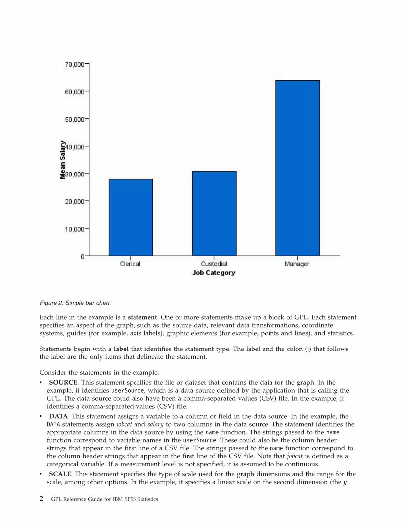
Each line in the example is a statement. One or more statements make up a block of GPL. Each statementspecifies an aspect of the graph, such as the source data, relevant data transformations, coordinatesystems, guides (for example, axis labels), graphic elements (for example, points and lines), and statistics.

Statements begin with a label that identifies the statement type. The label and the colon (:) that followsthe label are the only items that delineate the statement.

Consider the statements in the example:v SOURCE. This statement specifies the file or dataset that contains the data for the graph. In the

example, it identifies userSource, which is a data source defined by the application that is calling theGPL. The data source could also have been a comma-separated values (CSV) file. In the example, itidentifies a comma-separated values (CSV) file.

v DATA. This statement assigns a variable to a column or field in the data source. In the example, theDATA statements assign jobcat and salary to two columns in the data source. The statement identifies theappropriate columns in the data source by using the name function. The strings passed to the namefunction correspond to variable names in the userSource. These could also be the column headerstrings that appear in the first line of a CSV file. The strings passed to the name function correspond tothe column header strings that appear in the first line of the CSV file. Note that jobcat is defined as acategorical variable. If a measurement level is not specified, it is assumed to be continuous.

v SCALE. This statement specifies the type of scale used for the graph dimensions and the range for thescale, among other options. In the example, it specifies a linear scale on the second dimension (the y

Figure 2. Simple bar chart

2 GPL Reference Guide for IBM SPSS Statistics

axis in this case) and indicates that the scale must include 0. Linear scales do not necessarily include 0,but many bar charts do. Therefore, it's explicitly defined to ensure the bars start at 0. You need toinclude a SCALE statement only when you want to modify the scale. In this example, no SCALEstatement is specified for the first dimension. We are using the default scale, which is categoricalbecause the underlying data are categorical.

v GUIDE. This statement handles all of the aspects of the graph that aren't directly tied to the data buthelp to interpret the data, such as axis labels and reference lines. In the example, the GUIDE statementsspecify labels for the x and y axes. A specific axis is identified by a dim function. The first twodimensions of any graph are the x and y axes. The GUIDE statement is not required. Like the SCALEstatement, it is needed only when you want to modify a particular guide. In this case, we are addinglabels to the guides. The axis guides would still be created if the GUIDE statements were omitted, butthe axes would not have labels.

v ELEMENT. This statement identifies the graphic element type, variables, and statistics. The examplespecifies interval. An interval element is commonly known as a bar element. It creates the bars in theexample. position() specifies the location of the bars. One bar appears at each category in the jobcat.Because statistics are calculated on the second dimension in a 2-D graph, the height of the bars is themean of salary for each job category. The contents of position() use GPL algebra. See the topic “BriefOverview of GPL Algebra” for more information.

Details about all of the statements and functions appear in Chapter 2, “GPL Statement and FunctionReference,” on page 21.

GPL Syntax RulesWhen writing GPL, it is important to keep the following rules in mind.v Except in quoted strings, whitespace is irrelevant, including line breaks. Although it is possible to write

a complete GPL block on one line, line breaks are used for readability.v All quoted strings must be enclosed in quotation marks/double-quotes (for example, "text"). You

cannot use single quotes to enclose strings.v To add a quotation mark within a quoted string, precede the quotation mark with an escape character

(\) (for example, "Respondents Answering \"Yes\"").v To add a line break within a quoted string, use \n (for example, "Employment\nCategory").v GPL is case sensitive. Statement labels and function names must appear in the case as documented.

Other names (like variable names) are also case sensitive.v Functions are separated by commas. For example:

ELEMENT: point(position(x*y), color(z), size(size."5px"))

v GPL names must begin with an alpha character and can contain alphanumeric characters andunderscores (_), including those in international character sets. GPL names are used in the SOURCE,DATA, TRANS, and SCALE statements to assign the result of a function to the name. For example,gendervar in the following example is a GPL name:DATA: gendervar=col(source(s), name("gender"), unit.category())

GPL ConceptsThis section contains conceptual information about GPL. Although the information is useful forunderstanding GPL, it may not be easy to grasp unless you first review some examples. You can findexamples in Chapter 3, “GPL Examples,” on page 329.

Brief Overview of GPL AlgebraBefore you can use all of the functions and statements in GPL, it is important to understand its algebra.The algebra determines how data are combined to specify the position of graphic elements in the graph.That is, the algebra defines the graph dimensions or the data frame in which the graph is drawn. For

Chapter 1. Introduction to GPL 3

example, the frame of a basic scatterplot is specified by the values of one variable crossed with the valuesof another variable. Another way of thinking about the algebra is that it identifies the variables you wantto analyze in the graph.

The GPL algebra can specify one or more variables. If it includes more than one variable, you must useone of the following operators:v Cross (*). The cross operator crosses all of the values of one variable with all of the values of another

variable. A result exists for every case (row) in the data. The cross operator is the most commonly usedoperator. It is used whenever the graph includes more than one axis, with a different variable on eachaxis. Each variable on each axis is crossed with each variable on the other axes (for example, A*Bresults in A on the x axis and B on the y axis when the coordinate system is 2-D). Crossing can also beused for paneling (faceting) when there are more crossed variables than there are dimensions in acoordinate system. That is, if the coordinate system were 2-D rectangular and three variables werecrossed, the last variable would be used for paneling (for example, with A*B*C, C is used for panelingwhen the coordinate system is 2-D).

v Nest (/). The nest operator nests all of the values of one variable in all of the values of anothervariable. The difference between crossing and nesting is that a result exists only when there is acorresponding value in the variable that nests the other variable. For example, city/state nests the cityvariable in the state variable. A result will exist for each city and its appropriate state, not for everycombination of city and state. Therefore, there will not be a result for Chicago and Montana. Nestingalways results in paneling, regardless of the coordinate system.

v Blend (+). The blend operator combines all of the values of one variable with all of the values ofanother variable. For example, you may want to combine two salary variables on one axis. Blending isoften used for repeated measures, as in salary2004+salary2005.

Crossing and nesting add dimensions to the graph specification. Blending combines the values into onedimension. How the dimensions are interpreted and drawn depends on the coordinate system. See “HowCoordinates and the GPL Algebra Interact” on page 6 for details about the interaction between thecoordinate system and the algebra.

Rules

Like elementary mathematical algebra, GPL algebra has associative, distributive, and commutative rules.All operators are associative:(X*Y)*Z = X*(Y*Z)(X/Y)/Z = X/(Y/Z)(X+Y)+Z = X+(Y+Z)

The cross and nest operators are also distributive:X*(Y+Z) = X*Y+X*ZX/(Y+Z) = X/Y+X/Z

However, GPL algebra operators are not commutative. That is,X*Y ≠ Y*XX/Y ≠ Y/X

Operator Precedence

The nest operator takes precedence over the other operators, and the cross operator takes precedenceover the blend operator. Like mathematical algebra, the precedence can be changed by using parentheses.You will almost always use parentheses with the blend operator because the blend operator has thelowest precedence. For example, to blend variables before crossing or nesting the result with othervariables, you would do the following:(A+B)*C


However, note that there are some cases in which you will cross then blend. For example, consider thefollowing.(A*C)+(B*D)

In this case, the variables are crossed first because there is no way to untangle the variable values afterthey are blended. A needs to be crossed with C and B needs to be crossed with D. Therefore, using(A+B)*(C+D) won't work. (A*C)+(B*D) crosses the correct variables and then blends the results together.

Note: In this last example, the parentheses are superfluous, because the cross operator's higher precedenceensures that the crossing occurs before the blending. The parentheses are used for readability.

Analysis Variable

Statistics other than count-based statistics require an analysis variable. The analysis variable is thevariable on which a statistic is calculated. In a 1-D graph, this is the first variable in the algebra. In a 2-Dgraph, this is the second variable. Finally, in a 3-D graph, it is the third variable.

In all of the following, salary is the analysis variable:v 1-D. summary.sum(salary)

v 2-D. summary.mean(jobcat*salary)

v 3-D. summary.mean(jobcat*gender*salary)

The previous rules apply only to algebra used in the position function. Algebra can be used elsewhere(as in the color and label functions), in which case the only variable in the algebra is the analysisvariable. For example, in the following ELEMENT statement for a 2-D graph, the analysis variable is salaryin the position function and the label function.ELEMENT: interval(position(summary.mean(jobcat*salary)), label(summary.mean(salary)))

Unity Variable

The unity variable (indicated by 1) is a placeholder in the algebra. It is not the same as the numeric value1. When a scale is created for the unity variable, unity is located in the middle of the scale but no othervalues exist on the scale. The unity variable is needed only when there is no explicit variable in a specificdimension and you need to include the dimension in the algebra.

For example, assume a 2-D rectangular coordinate system. If you are creating a graph showing the countin each jobcat category, summary.count(jobcat) appears in the GPL specification. Counts are shown alongthe y axis, but there is no explicit variable in that dimension. If you want to panel the graph, you need tospecify something in the second dimension before you can include the paneling variable. Thus, if youwant to panel the graph by columns using gender, you need to change the specification tosummary.count(jobcat*1*gender). If you want to panel by rows instead, there would be another unityvariable to indicate the missing third dimension. The specification would change tosummary.count(jobcat*1*1*gender).

You can't use the unity variable to compute statistics that require an analysis variable (like summary.mean).However, you can use it with count-based statistics (like summary.count and summary.percent.count).

User Constants

The algebra can also include user constants, which are quoted string values (for example, "2005"). Whena user constant is included in the algebra, it is like adding a new variable, with the variable's value equalto the constant for all cases. The effect of this depends on the algebra operators and the function in whichthe user constant appears.


In the position function, the constants can be used to create separate scales. For example, in thefollowing GPL, two separate scales are created for the paneled graph. By nesting the values of eachvariable in a different string and blending the results, two different groups of cases with different scaleranges are created.ELEMENT: line(position(date*(calls/"Calls"+orders/"Orders")))

For a full example, see “Line Chart with Separate Scales” on page 384.

If the cross operator is used instead of the nest operator, both categories will have the same scale range.The panel structures will also differ.ELEMENT: line(position(date*calls*"Calls"+date*orders*"Orders"))

Constants can also be used in the position function to create a category of all cases when the constant isblended with a categorical variable. Remember that the value of the user constant is applied to all cases,so that's why the following works:ELEMENT: interval(position(summary.mean((jobcat+"All")*salary)))

For a full example, see “Simple Bar Chart with Bar for All Categories” on page 334.

Aesthetic functions can also take advantage of user constants. Blending variables creates multiple graphicelements for the same case. To distinguish each group, you can mimic the blending in the aestheticfunction—this time with user constants.ELEMENT: point(position(jobcat*(salbegin+salary), color("Beginning"+"Current")))

User constants are not required to create most charts, so you can ignore them in the beginning. However,as you become more proficient with GPL, you may want to return to them to create custom graphs.

How Coordinates and the GPL Algebra InteractThe algebra defines the dimensions of the graph. Each crossing results in an additional dimension. Thus,gender*jobcat*salary specifies three dimensions. How these dimensions are drawn depends on thecoordinate system and any functions that may modify the coordinate system.

Some examples may clarify these concepts. The relevant GPL statements are extracted from the fullspecification.

1-D GraphCOORD: rect(dim(1))ELEMENT: point(position(salary))

Full SpecificationSOURCE: s = csvSource(file("Employee data.csv"))DATA: salary = col(source(s), name("salary"))COORD: rect(dim(1))GUIDE: axis(dim(1), label("Salary"))ELEMENT: point(position(salary))

SOURCE: s = userSource(id("Employeedata"))DATA: salary = col(source(s), name("salary"))COORD: rect(dim(1))GUIDE: axis(dim(1), label("Salary"))ELEMENT: point(position(salary))


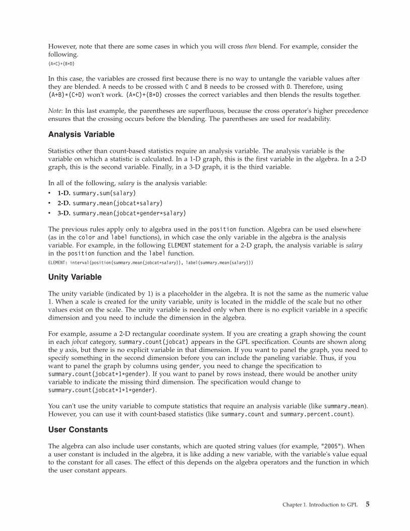
v The coordinate system is explicitly set to one-dimensional, and only one variable appears in thealgebra.

v The variable is plotted on one dimension.

2-D GraphELEMENT: point(position(salbegin*salary))

Full SpecificationSOURCE: s = csvSource(file("Employee data.csv"))DATA: salbegin=col(source(s), name("salbegin"))DATA: salary=col(source(s), name("salary"))GUIDE: axis(dim(2), label("Current Salary"))GUIDE: axis(dim(1), label("Beginning Salary"))ELEMENT: point(position(salbegin*salary))

SOURCE: s = userSource(id("Employeedata"))DATA: salbegin=col(source(s), name("salbegin"))DATA: salary=col(source(s), name("salary"))GUIDE: axis(dim(2), label("Current Salary"))GUIDE: axis(dim(1), label("Beginning Salary"))ELEMENT: point(position(salbegin*salary))

Figure 3. Simple 1-D scatterplot


v No coordinate system is specified, so it is assumed to be 2-D rectangular.v The two crossed variables are plotted against each other.

Another 2-D GraphELEMENT: interval(position(summary.count(jobcat)))

Full SpecificationSOURCE: s = csvSource(file("Employee data.csv"))DATA: jobcat=col(source(s), name("jobcat"), unit.category())SCALE: linear(dim(2), include(0))GUIDE: axis(dim(2), label("Count"))GUIDE: axis(dim(1), label("Job Category"))ELEMENT: interval(position(summary.count(jobcat)))

SOURCE: s = userSource(id("Employeedata"))DATA: jobcat=col(source(s), name("jobcat"), unit.category())SCALE: linear(dim(2), include(0))GUIDE: axis(dim(2), label("Count"))GUIDE: axis(dim(1), label("Job Category"))ELEMENT: interval(position(summary.count(jobcat)))



v No coordinate system is specified, so it is assumed to be 2-D rectangular.v Although there is only one variable in the specification, another for the result of the count statistic is

implied (percent statistics behave similarly). The algebra could have been written as jobcat*1.v The variable and the result of the statistic are plotted.

A Faceted (Paneled) 2-D GraphELEMENT: interval(position(summary.mean(jobcat*salary*gender)))

Full SpecificationSOURCE: s = csvSource(file("Employee data.csv"))DATA: jobcat = col(source(s), name("jobcat"), unit.category())DATA: gender = col(source(s), name("gender"), unit.category())DATA: salary = col(source(s), name("salary"))SCALE: linear(dim(2), include(0))GUIDE: axis(dim(3), label("Gender"))GUIDE: axis(dim(2), label("Mean Salary"))GUIDE: axis(dim(1), label("Job Category"))ELEMENT: interval(position(summary.mean(jobcat*salary*gender)))

SOURCE: s = userSource(id("Employeedata"))DATA: jobcat = col(source(s), name("jobcat"), unit.category())DATA: gender = col(source(s), name("gender"), unit.category())DATA: salary = col(source(s), name("salary"))SCALE: linear(dim(2), include(0))

Figure 5. Simple 2-D bar chart of counts


GUIDE: axis(dim(3), label("Gender"))GUIDE: axis(dim(2), label("Mean Salary"))GUIDE: axis(dim(1), label("Job Category"))ELEMENT: interval(position(summary.mean(jobcat*salary*gender)))

v No coordinate system is specified, so it is assumed to be 2-D rectangular.v There are three variables in the algebra, but only two dimensions. The last variable is used for faceting

(also known as paneling).v The second dimension variable in a 2-D chart is the analysis variable. That is, it is the variable on

which the statistic is calculated.v The first variable is plotted against the result of the summary statistic calculated on the second variable

for each category in the faceting variable.

A Faceted (Paneled) 2-D Graph with Nested CategoriesELEMENT: interval(position(summary.mean(jobcat/gender*salary)))

Full SpecificationSOURCE: s = csvSource(file("Employee data.csv"))DATA: jobcat = col(source(s), name("jobcat"), unit.category())DATA: gender = col(source(s), name("gender"), unit.category())DATA: salary = col(source(s), name("salary"))SCALE: linear(dim(2), include(0.0))GUIDE: axis(dim(2), label("Mean Salary"))GUIDE: axis(dim(1.1), label("Job Category"))GUIDE: axis(dim(1), label("Gender"))ELEMENT: interval(position(summary.mean(jobcat/gender*salary)))

SOURCE: s = userSource(id("Employeedata"))DATA: jobcat = col(source(s), name("jobcat"), unit.category())DATA: gender = col(source(s), name("gender"), unit.category())DATA: salary = col(source(s), name("salary"))

Figure 6. Faceted 2-D bar chart


SCALE: linear(dim(2), include(0.0))GUIDE: axis(dim(2), label("Mean Salary"))GUIDE: axis(dim(1.1), label("Job Category"))GUIDE: axis(dim(1), label("Gender"))ELEMENT: interval(position(summary.mean(jobcat/gender*salary)))

v This example is the same as the previous paneled example, except for the algebra.v The second dimension variable is the same as in the previous example. Therefore, it is the variable on

which the statistic is calculated.v jobcat is nested in gender. Nesting always results in faceting, regardless of the available dimensions.v With nested categories, only those combinations of categories that occur in the data are shown in the

graph. In this case, there is no bar for Female and Custodial in the graph, because there is no case withthis combination of categories in the data. Compare this result to the previous example that createdfacets by crossing categorical variables.

A 3-D GraphCOORD: rect(dim(1,2,3))ELEMENT: interval(position(summary.mean(jobcat*gender*salary)))

Full SpecificationSOURCE: s = csvSource(file("Employee data.csv"))DATA: jobcat=col(source(s), name("jobcat"), unit.category())DATA: gender=col(source(s), name("gender"), unit.category())DATA: salary=col(source(s), name("salary"))COORD: rect(dim(1,2,3))SCALE: linear(dim(3), include(0))GUIDE: axis(dim(3), label("Mean Salary"))GUIDE: axis(dim(2), label("Gender"))GUIDE: axis(dim(1), label("Job Category"))ELEMENT: interval(position(summary.mean(jobcat*gender*salary)))

Figure 7. Faceted 2-D bar chart with nested categories


SOURCE: s = userSource(id("Employeedata"))DATA: jobcat=col(source(s), name("jobcat"), unit.category())DATA: gender=col(source(s), name("gender"), unit.category())DATA: salary=col(source(s), name("salary"))COORD: rect(dim(1,2,3))SCALE: linear(dim(3), include(0))GUIDE: axis(dim(3), label("Mean Salary"))GUIDE: axis(dim(2), label("Gender"))GUIDE: axis(dim(1), label("Job Category"))ELEMENT: interval(position(summary.mean(jobcat*gender*salary)))

v The coordinate system is explicitly set to three-dimensional, and there are three variables in thealgebra.

v The three variables are plotted on the available dimensions.v The third dimension variable in a 3-D chart is the analysis variable. This differs from the 2-D chart in

which the second dimension variable is the analysis variable.

A Clustered GraphCOORD: rect(dim(1,2), cluster(3))ELEMENT: interval(position(summary.mean(gender*salary*jobcat)), color(gender))

Full Specification

Figure 8. 3-D bar chart


SOURCE: s = csvSource(file("Employee data.csv"))DATA: jobcat=col(source(s), name("jobcat"), unit.category())DATA: gender=col(source(s), name("gender"), unit.category())DATA: salary=col(source(s), name("salary"))COORD: rect(dim(1,2), cluster(3))SCALE: linear(dim(2), include(0))GUIDE: axis(dim(2), label("Mean Salary"))GUIDE: axis(dim(3), label("Gender"))ELEMENT: interval(position(summary.mean(jobcat*salary*gender)), color(jobcat))

SOURCE: s = userSource(id("Employeedata"))DATA: jobcat=col(source(s), name("jobcat"), unit.category())DATA: gender=col(source(s), name("gender"), unit.category())DATA: salary=col(source(s), name("salary"))COORD: rect(dim(1,2), cluster(3))SCALE: linear(dim(2), include(0))GUIDE: axis(dim(2), label("Mean Salary"))GUIDE: axis(dim(3), label("Gender"))ELEMENT: interval(position(summary.mean(jobcat*salary*gender)), color(jobcat))

v The coordinate system is explicitly set to two-dimensional, but it is modified by the cluster function.v The cluster function indicates that clustering occurs along dim(3), which is the dimension associated

with jobcat because it is the third variable in the algebra.v The variable in dim(1) identifies the variable whose values determine the bars in each cluster. This is

gender.v Although the coordinate system was modified, this is still a 2-D chart. Therefore, the analysis variable

is still the second dimension variable.v The variables are plotted using the modified coordinate system. Note that the graph would be a

paneled graph if you removed the cluster function. The charts would look similar and show the sameresults, but their coordinate systems would differ. Refer back to the paneled 2-D graph to see thedifference.

Figure 9. Clustered 2-D bar chart


Common TasksThis section provides information for adding common graph features. This GPL creates a simple 2-D barchart. You can apply the steps to any graph, but the examples use the GPL in “The Basics” on page 1 as a"baseline."

How to Add Stacking to a GraphStacking involves a couple of changes to the ELEMENT statement. The following steps use the GPL shownin “The Basics” on page 1 as a "baseline" for the changes.1. Before modifying the ELEMENT statement, you need to define an additional categorical variable that will

be used for stacking. This is specified by a DATA statement (note the unit.category() function):DATA: gender=col(source(s), name("gender"), unit.category())

2. The first change to the ELEMENT statement will split the graphic element into color groups for eachgender category. This splitting results from using the color function:ELEMENT: interval(position(summary.mean(jobcat*salary)), color(gender))

3. Because there is no collision modifier for the interval element, the groups of bars are overlaid on eachother, and there's no way to distinguish them. In fact, you may not even see graphic elements for oneof the groups because the other graphic elements obscure them. You need to add the stacking collisionmodifier to re-position the groups (we also changed the statistic because stacking summed valuesmakes more sense than stacking the mean values):

ELEMENT: interval.stack(position(summary.sum(jobcat*salary)), color(gender))

The complete GPL is shown below:SOURCE: s = csvSource(file("Employee data.csv"))DATA: jobcat = col(source(s), name("jobcat"), unit.category())DATA: gender = col(source(s), name("gender"), unit.category())DATA: salary = col(source(s), name("salary"))SCALE: linear(dim(2), include(0.0))GUIDE: axis(dim(2), label("Sum Salary"))GUIDE: axis(dim(1), label("Job Category"))ELEMENT: interval.stack(position(summary.sum(jobcat*salary)), color(gender))

SOURCE: s = userSource(id("Employeedata"))DATA: jobcat = col(source(s), name("jobcat"), unit.category())DATA: gender = col(source(s), name("gender"), unit.category())DATA: salary = col(source(s), name("salary"))SCALE: linear(dim(2), include(0.0))GUIDE: axis(dim(2), label("Sum Salary"))GUIDE: axis(dim(1), label("Job Category"))ELEMENT: interval.stack(position(summary.sum(jobcat*salary)), color(gender))

Following is the graph created from the GPL.


Legend Label

The graph includes a legend, but it has no label by default. To add or change the label for the legend,you use a GUIDE statement:GUIDE: legend(aesthetic(aesthetic.color), label("Gender"))

How to Add Faceting (Paneling) to a GraphFaceted variables are added to the algebra in the ELEMENT statement. The following steps use the GPLshown in “The Basics” on page 1 as a "baseline" for the changes.1. Before modifying the ELEMENT statement, we need to define an additional categorical variable that will

be used for faceting. This is specified by a DATA statement (note the unit.category() function):DATA: gender=col(source(s), name("gender"), unit.category())

2. Now we add the variable to the algebra. We will cross the variable with the other variables in thealgebra:

ELEMENT: interval(position(summary.mean(jobcat*salary*gender)))

Those are the only necessary steps. The final GPL is shown below.SOURCE: s = csvSource(file("Employee data.csv"))DATA: jobcat = col(source(s), name("jobcat"), unit.category())DATA: gender = col(source(s), name("gender"), unit.category())DATA: salary = col(source(s), name("salary"))SCALE: linear(dim(2), include(0.0))GUIDE: axis(dim(2), label("Mean Salary"))GUIDE: axis(dim(1), label("Job Category"))ELEMENT: interval(position(summary.mean(jobcat*salary*gender)))

SOURCE: s = userSource(id("Employeedata"))DATA: jobcat = col(source(s), name("jobcat"), unit.category())DATA: gender = col(source(s), name("gender"), unit.category())DATA: salary = col(source(s), name("salary"))

Figure 10. Stacked bar chart


SCALE: linear(dim(2), include(0.0))GUIDE: axis(dim(2), label("Mean Salary"))GUIDE: axis(dim(1), label("Job Category"))ELEMENT: interval(position(summary.mean(jobcat*salary*gender)))


Additional Features

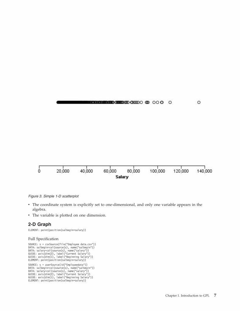
Labeling. If you want to label the faceted dimension, you treat it like the other dimensions in the graphby adding a GUIDE statement for its axis:GUIDE: axis(dim(3), label("Gender"))

In this case, it is specified as the 3rd dimension. You can determine the dimension number by countingthe crossed variables in the algebra. gender is the 3rd variable.

Nesting. Faceted variables can be nested as well as crossed. Unlike crossed variables, the nested variableis positioned next to the variable in which it is nested. So, to nest gender in jobcat, you would do thefollowing:ELEMENT: interval(position(summary.mean(jobcat/gender*salary)))

Because gender is used for nesting, it is not the 3rd dimension as it was when crossing to create facets.You can't use the same simple counting method to determine the dimension number. You still count thecrossings, but you count each crossing as a single factor. The number that you obtain by counting eachcrossed factor is used for the nested variable (in this case, 1). The other dimension is indicated by thenested variable dimension followed by a dot and the number 1 (in this case, 1.1). So, you would use thefollowing convention to refer to the gender and jobcat dimensions in the GUIDE statement:

Figure 11. Faceted bar chart


GUIDE: axis(dim(1), label("Gender"))GUIDE: axis(dim(1.1), label("Job Category"))GUIDE: axis(dim(2), label("Mean Salary"))

How to Add Clustering to a GraphClustering involves changes to the COORD statement and the ELEMENT statement. The following steps usethe GPL shown in “The Basics” on page 1 as a "baseline" for the changes.1. Before modifying the COORD and ELEMENT statements, you need to define an additional categorical

variable that will be used for clustering. This is specified by a DATA statement (note theunit.category() function):DATA: gender=col(source(s), name("gender"), unit.category())

2. Now you will modify the COORD statement. If, like the baseline graph, the GPL does not alreadyinclude a COORD statement, you first need to add one:COORD: rect(dim(1,2))

In this case, the default coordinate system is now explicit.3. Next add the cluster function to the coordinate system and specify the clustering dimension. In a 2-D

coordinate system, this is the third dimension:COORD: rect(dim(1,2), cluster(3))

4. Now we add the clustering dimension variable to the algebra. This variable is in the 3rd position,corresponding to the clustering dimension specified by the cluster function in the COORD statement:ELEMENT: interval(position(summary.mean(jobcat*salary*gender)))

Note that this algebra looks similar to the algebra for faceting. Without the cluster function added inthe previous step, the resulting graph would be faceted. The cluster function essentially collapses thefaceting into one axis. Instead of a facet for each gender category, there is a cluster on the x axis foreach category.

5. Because clustering changes the dimensions, we update the GUIDE statement so that it corresponds tothe clustering dimension.GUIDE: axis(dim(3), label("Gender"))

6. With these changes, the chart is clustered, but there is no way to distinguish the bars in each cluster.You need to add an aesthetic to distinguish the bars:

ELEMENT: interval(position(summary.mean(jobcat*salary*gender)), color(jobcat))

The complete GPL looks like the following.SOURCE: s = csvSource(file("Employee data.csv"))DATA: jobcat=col(source(s), name("jobcat"), unit.category())DATA: gender=col(source(s), name("gender"), unit.category())DATA: salary=col(source(s), name("salary"))COORD: rect(dim(1,2), cluster(3))SCALE: linear(dim(2), include(0))GUIDE: axis(dim(2), label("Mean Salary"))GUIDE: axis(dim(3), label("Gender"))ELEMENT: interval(position(summary.mean(jobcat*salary*gender)), color(jobcat))




Legend Label

The graph includes a legend, but it has no label by default. To change the label for the legend, you use aGUIDE statement:GUIDE: legend(aesthetic(aesthetic.color), label("Gender"))

How to Use AestheticsGPL includes several different aesthetic functions for controlling the appearance of a graphic element. Thesimplest use of an aesthetic function is to define a uniform aesthetic for every instance of a graphicelement. For example, you can use the color function to assign a color constant (like color.red) to thepoint element, thereby making all of the points in the graph red.

A more interesting use of an aesthetic function is to change the value of the aesthetic based on the valueof another variable. For example, instead of a uniform color for the scatterplot points, the color couldvary based on the value of the categorical variable gender. All of the points in the Male category will beone color, and all of the points in the Female category will be another. Using a categorical variable for anaesthetic creates groups of cases. In addition to identifying the graphic elements for the groups of cases,the grouping allows you to evaluate statistics for the individual groups, if needed.

An aesthetic may also vary based on a set of continuous values. Using continuous values for the aestheticdoes not result in distinct groups of graphic elements. Instead, the aesthetic varies along the samecontinuous scale. There are no distinct groups on the scale, so the color varies gradually, just as thecontinuous values do.

Figure 12. Clustered bar chart


The steps below use the following GPL as a "baseline" for adding the aesthetics. This GPL creates asimple scatterplot.

1. First, you need to define an additional categorical variable that will be used for one of the aesthetics.This is specified by a DATA statement (note the unit.category() function):DATA: gender=col(source(s), name("gender"), unit.category())

2. Next you need to define another variable, this one being continuous. It will be used for the otheraesthetic.DATA: prevexp=col(source(s), name("prevexp"))

3. Now you will add the aesthetics to the graphic element in the ELEMENT statement. First add theaesthetic for the categorical variable:ELEMENT: point(position(salbegin*salary), shape(gender))

Shape is a good aesthetic for the categorical variable. It has distinct values that correspond well tocategorical values.

4. Finally add the aesthetic for the continuous variable:ELEMENT: point(position(salbegin*salary), shape(gender), color(prevexp))

Not all aesthetics are available for continuous variables. That's another reason why shape was a goodaesthetic for the categorical variable. Shape is not available for continuous variables because therearen't enough shapes to cover a continuous spectrum. On the other hand, color gradually changes inthe graph. It can capture the full spectrum of continuous values. Transparency or brightness wouldalso work well.

The complete GPL looks like the following.SOURCE: s = csvSource(file("Employee data.csv"))DATA: salbegin = col(source(s), name("salbegin"))DATA: salary = col(source(s), name("salary"))DATA: gender = col(source(s), name("gender"), unit.category())DATA: prevexp = col(source(s), name("prevexp"))GUIDE: axis(dim(2), label("Current Salary"))GUIDE: axis(dim(1), label("Beginning Salary"))ELEMENT: point(position(salbegin*salary), shape(gender), color(prevexp))

SOURCE: s = userSource(id("Employeedata"))DATA: salbegin = col(source(s), name("salbegin"))DATA: salary = col(source(s), name("salary"))DATA: gender = col(source(s), name("gender"), unit.category())DATA: prevexp = col(source(s), name("prevexp"))GUIDE: axis(dim(2), label("Current Salary"))GUIDE: axis(dim(1), label("Beginning Salary"))ELEMENT: point(position(salbegin*salary), shape(gender), color(prevexp))


SOURCE: s = csvSource(file("Employee data.csv"))DATA: salbegin=col(source(s), name("salbegin"))DATA: salary=col(source(s), name("salary"))GUIDE: axis(dim(2), label("Current Salary"))GUIDE: axis(dim(1), label("Beginning Salary"))ELEMENT: point(position(salbegin*salary))


Figure 13. Baseline GPL for example


Legend Label

The graph includes legends, but the legends have no labels by default. To change the labels, you useGUIDE statements that reference each aesthetic:GUIDE: legend(aesthetic(aesthetic.shape), label("Gender"))GUIDE: legend(aesthetic(aesthetic.color), label("Previous Experience"))

When interpreting the color legend in the example, it's important to realize that the color aestheticcorresponds to a continuous variable. Only a handful of colors may be shown in the legend, and thesecolors do not reflect the whole spectrum of colors that could appear in the graph itself. They are morelike mileposts at major divisions.

Figure 14. Scatterplot with aesthetics


Chapter 2. GPL Statement and Function Reference

This section provides detailed information about the various statements that make up GPL and thefunctions that you can use in each of the statements.

GPL StatementsThere are general categories of GPL statements.

Data definition statements. Data definition statements specify the data sources, variables, and optionalvariable transformations. All GPL code blocks include at least two data definition statements: one todefine the actual data source and one to specify the variable extracted from the data source.

Specification statements. Specification statements define the graph. They define the axis scales,coordinate systems, text, graphic elements (for example, bars and points), and statistics. All GPL codeblocks require at least one ELEMENT statement, but the other specification statements are optional. GPLuses a default value when the SCALE, COORD, and GUIDE statements are not included in the GPL code block.

Control statements. Control statements specify the layout for graphs. The GRAPH statement allows you togroup multiple graphs in a single page display. For example, you may want to add histograms to theborders on a scatterplot. The PAGE statement allows you to set the size of the overall visualization.Control statements are optional.

Comment statement. The COMMENT statement is used for adding comments to the GPL. These are optional.Data Definition Statements

“SOURCE Statement” on page 23“DATA Statement” on page 24“TRANS Statement” on page 24Specification Statements

“COORD Statement” on page 25“SCALE Statement” on page 29“GUIDE Statement” on page 41“ELEMENT Statement” on page 46Control Statements

“PAGE Statement” on page 22“GRAPH Statement” on page 22Comment Statements

“COMMENT Statement”

COMMENT StatementSyntaxCOMMENT: <text>

<text>. The comment text. This can consist of any string of characters except a statement label followedby a colon (:), unless the statement label and colon are enclosed in quotes (for example, COMMENT: With"SCALE:" statement).

Description

© Copyright IBM Corporation 1989, 2013 21

This statement is optional. You can use it to add comments to your GPL or to comment out a statementby converting it to a comment. The comment does not appear in the resulting graph.

Examples

PAGE StatementSyntaxPAGE: <function>

<function>. A function for specifying the PAGE statements that mark the beginning and end of thevisualization.

Description

This statement is optional. It's needed only when you specify a size for the page display or visualization.The current release of GPL supports only one PAGE block.

If you are using GRAPH blocks in a PAGE block, note the following:v SOURCE and DATA statements must appear directly in the PAGE block, followed by the GRAPH blocks. (See

the second example, "Defining a page with multiple graphs.")v TRANS, COORD, SCALE, GUIDE, and ELEMENT statements cannot appear directly in the PAGE block. These

statements apply to individual graphs and must appear in the GRAPH block to which they apply.

Examples

Valid Functions

“begin Function (For GPL Pages)” on page 69“end Function” on page 125

GRAPH StatementSyntaxGRAPH: <function>

COMMENT: This graph shows counts for each job category.

Figure 15. Defining a comment

PAGE: begin(scale(400px,300px))SOURCE: s=csvSource(file("mydata.csv"))DATA: x=col(source(s), name("x"))DATA: y=col(source(s), name("y"))ELEMENT: line(position(x*y))PAGE: end()

Figure 16. Example: Defining a page

PAGE: begin(scale(400px,300px))SOURCE: s=csvSource(file("mydata.csv"))DATA: a=col(source(s), name("a"))DATA: b=col(source(s), name("b"))DATA: c=col(source(s), name("c"))GRAPH: begin(scale(90%, 45%), origin(10%, 50%))ELEMENT: line(position(a*c))GRAPH: end()GRAPH: begin(scale(90%, 45%), origin(10%, 0%))ELEMENT: line(position(b*c))GRAPH: end()PAGE: end()

Figure 17. Example: Defining a page with multiple graphs


<function>. A function for specifying the GRAPH statements that mark the beginning and end of theindividual graph.

Description

This statement is optional. It's needed only when you want to group multiple graphs in a single pagedisplay or you want to customize a graph's size. The GRAPH statement is essentially a wrapper around theGPL that defines a particular graph. There is no limit to the number of graphs that can appear in a GPLblock.

Grouping graphs is useful for related graphs, like graphs on the borders of histograms. However, thegraphs do not have to be related. You may simply want to group the graphs for presentation.

For information about organization of statements when there are multiple GRAPH statements, see “PAGEStatement” on page 22.

Examples

Valid Functions

“begin Function (For GPL Graphs)” on page 69“end Function” on page 125

SOURCE StatementSyntaxSOURCE: <source name> = <function>

<source name>. User-defined name for the data source. Refer to “GPL Syntax Rules” on page 3 forinformation about which characters you can use in the name.

<function>. A function for extracting data from various data sources.

Description

Defines a data source for the graph. There can be multiple data sources, each specified by a differentSOURCE statement.

Examples

Valid Functions

GRAPH: begin(scale(50%,50%))

Figure 18. Scaling a graph

GRAPH: begin(origin(10.0%, 20.0%), scale(80.0%, 80.0%))ELEMENT: point(position(salbegin*salary))GRAPH: end()GRAPH: begin(origin(10.0%, 100.0%), scale(80.0%, 10.0%))ELEMENT: interval(position(summary.count(bin.rect(salbegin))))GRAPH: end()GRAPH: begin(origin(90.0%, 20.0%), scale(10.0%, 80.0%))COORD: transpose()ELEMENT: interval(position(summary.count(bin.rect(salary))))GRAPH: end()

Figure 19. Example: Scatterplot with border histograms

SOURCE: mydata = csvSource(path("/Data/demo.csv"))

Figure 20. Example: Reading a CSV file

Chapter 2. GPL Statement and Function Reference 23

“csvSource Function” on page 92“savSource Function” on page 216“sqlSource Function” on page 243“userSource Function” on page 324

DATA StatementSyntaxDATA: <variable name> = <function>

<variable name>. User-defined name for the variable. Refer to “GPL Syntax Rules” on page 3 forinformation about which characters you can use in the name.

<function>. A function indicating the data sources.

Description

Defines a variable from a specific data source. The GPL statement must also include a SOURCE statement.The name identified by the SOURCE statement is used in the DATA statement to indicate the data sourcefrom which a particular variable is extracted.

Examples

age is an arbitrary name. In this example, the variable name is the same as the name that appears in thedata source. Using the same name avoids confusion. The col function takes a data source and data sourcevariable name as its arguments. Note that the data source name was previously defined by a SOURCEstatement and is not enclosed in quotes.

Valid Functions

“col Function” on page 84“iter Function” on page 136

TRANS StatementSyntaxTRANS: <variable name> = <function>

<variable name>. A string that specifies a name for the variable that is created as a result of thetransformation. Refer to “GPL Syntax Rules” on page 3 for information about which characters you canuse in the name.

<function>. A valid function.

Description

Defines a new variable whose value is the result of a data transformation function.

Examples

DATA: age = col(source(mydata), name("age"))

Figure 21. Example: Specifying a variable from a data source

TRANS: saldiff = eval(((salary-salbegin)/salary)*100)

Figure 22. Example: Creating a transformation variable from other variables


Valid Functions

“collapse Function” on page 85“eval Function” on page 126“index Function” on page 136

COORD StatementSyntaxCOORD: <coord>

<coord>. A valid coordinate type or transformation function.

Description

Specifies a coordinate system for the graph. You can also embed coordinate systems or wrap a coordinatesystem in a transformation. When transformations and coordinate systems are embedded in each other,they are applied in order, with the innermost being applied first. Thus, mirror(transpose(rect(1,2)))specifies that a 2-D rectangular coordinate system is transposed and then mirrored.

Examples

Coordinate Types and Transformations

“parallel Coordinate Type” on page 26“polar Coordinate Type” on page 26“polar.theta Coordinate Type” on page 27“rect Coordinate Type” on page 28“mirror Function” on page 186“project Function” on page 194“reflect Function” on page 195“transpose Function” on page 323“wrap Function” on page 327

GPL Coordinate TypesThere are several coordinate types available in GPL.

Coordinate Types

“parallel Coordinate Type” on page 26“polar Coordinate Type” on page 26

TRANS: casenum = index()

Figure 23. Example: Creating an index variable

COORD: polar.theta()

Figure 24. Example: Polar coordinates for pie charts

COORD: rect(dim(1,2,3))

Figure 25. Example: 3-D rectangular coordinates

COORD: rect(dim(2), polar.theta(dim(1)))

Figure 26. Example: Embedded coordinate systems for paneled pie chart

COORD: transpose()

Figure 27. Example: Transposed coordinate system


“polar.theta Coordinate Type” on page 27“rect Coordinate Type” on page 28

parallel Coordinate Type: Syntaxparallel(dim(<numeric>), <coord>)

<numeric>. One or more numeric values (separated by commas) indicating the graph dimension ordimensions to which the parallel coordinate system applies. The number of values equals the number ofdimensions for the coordinate system's frame, and the values are always in sequential order. For example,parallel(dim(1,2,3,4)) indicates that the first four variables in the algebra are used for the parallelcoordinates. Any others are used for faceting. If no dimensions are specified, all variables are used for theparallel coordinates. See the topic “dim Function” on page 124 for more information.

<coord>. A valid coordinate type or transformation function. This is optional.

Description

Creates a parallel coordinate system. A graph using this coordinate system consists of multiple, parallelaxes showing data across multiple variables, resulting in a plot that is similar to a profile plot.

When you use a parallel coordinate system, you cross each continuous variable in the algebra. A linegraphic element is the most common element type for this graph. The graphic element is alwaysdistinguished by some aesthetic so that any patterns are readily apparent.

Examples


“polar Coordinate Type”“polar.theta Coordinate Type” on page 27“rect Coordinate Type” on page 28“mirror Function” on page 186“project Function” on page 194“reflect Function” on page 195“transpose Function” on page 323“wrap Function” on page 327Applies To

“COORD Statement” on page 25“polar Coordinate Type”“polar.theta Coordinate Type” on page 27“rect Coordinate Type” on page 28“project Function” on page 194

polar Coordinate Type: Syntaxpolar(dim(<numeric>), <function>, <coord>)

TRANS: caseid = index()COORD: parallel()ELEMENT: line(position(var1*var2*var3*var4), split(caseid), color(catvar1))

The example includes the split function to create a separate line for each case in the data. Otherwise, there would beonly one line that crossed back through the coordinate system to connect all the cases.Figure 28. Example: Parallel coordinates graph


<numeric>. Numeric values (separated by commas) indicating the dimensions to which the polarcoordinates apply. This is optional and is assumed to be the first two dimensions. See the topic “dimFunction” on page 124 for more information.

<function>. One or more valid functions. These are optional.


Description

Creates a polar coordinate system. This differs from the polar.theta coordinate system in that it is twodimensional. One dimension is associated with the radius, and the other is associated with the thetaangle.

Examples

Valid Functions

“reverse Function” on page 214“startAngle Function” on page 244Coordinate Types and Transformations

“parallel Coordinate Type” on page 26“polar.theta Coordinate Type”“rect Coordinate Type” on page 28“mirror Function” on page 186“project Function” on page 194“reflect Function” on page 195“transpose Function” on page 323“wrap Function” on page 327Applies To

“COORD Statement” on page 25“parallel Coordinate Type” on page 26“polar.theta Coordinate Type”“rect Coordinate Type” on page 28“project Function” on page 194

polar.theta Coordinate Type: Syntaxpolar.theta(<function>, <coord>)

<numeric>. A numeric value indicating the dimension. This is optional and required only whenpolar.theta is not the first or innermost dimension. Otherwise, it is assumed to be the first dimension.See the topic “dim Function” on page 124 for more information.



Description

COORD: polar()ELEMENT: line(position(date*close), closed(), preserveStraightLines())

Figure 29. Example: Polar line chart


Creates a polar.theta coordinate system, which is the coordinate system for creating pie charts. polar.thetadiffers from the polar coordinate system in that it is one dimensional. This is the dimension for the thetaangle.

Examples

Valid Functions

“reverse Function” on page 214“startAngle Function” on page 244Coordinate Types and Transformations

“parallel Coordinate Type” on page 26“polar Coordinate Type” on page 26“rect Coordinate Type”“mirror Function” on page 186“project Function” on page 194“reflect Function” on page 195“transpose Function” on page 323“wrap Function” on page 327Applies To

“COORD Statement” on page 25“parallel Coordinate Type” on page 26“polar Coordinate Type” on page 26“rect Coordinate Type”“project Function” on page 194

rect Coordinate Type: Syntaxrect(dim(<numeric>), <function>, <coord>)

<numeric>. One or more numeric values (separated by commas) indicating the graph dimension ordimensions to which the rectangular coordinate system applies. The number of values equals the numberof dimensions for the coordinate system's frame, and the values are always in sequential order (forexample, dim(1,2,3) and dim(4,5)). See the topic “dim Function” on page 124 for more information.



Description

Creates a rectangular coordinate system. By default, a rectangular coordinate system is 2-D, which is theequivalent of specifying rect(dim(1,2)). To create a 3-D coordinate system, use rect(dim(1,2,3)).Similarly, use rect(dim(1)) to specify a 1-D coordinate system. Changing the coordinate system alsochanges which variable in the algebra is summarized for a statistic. The statistic function is calculated onthe second crossed variable in a 2-D coordinate system and the third crossed variable in a 3-D coordinatesystem.

Examples

COORD: polar.theta()ELEMENT: interval.stack(position(summary.count()), color(jobcat))

Figure 30. Example: Pie chart


Valid Functions

“cluster Function” on page 82“sameRatio Function” on page 215Coordinate Types and Transformations

“parallel Coordinate Type” on page 26“polar Coordinate Type” on page 26“polar.theta Coordinate Type” on page 27“mirror Function” on page 186“project Function” on page 194“reflect Function” on page 195“transpose Function” on page 323“wrap Function” on page 327Applies To

“COORD Statement” on page 25“parallel Coordinate Type” on page 26“polar Coordinate Type” on page 26“polar.theta Coordinate Type” on page 27“project Function” on page 194

SCALE StatementSyntaxSCALE: <scale type>

orSCALE: <scale name> = <scale type>

<scale type>. A valid scale type.

<scale name>. A user-defined name for the scale. This is required only when you are creating a graphwith dual scales. An example is a graph that shows the mean of a variable on one axis and the count onthe other. The scale name is referenced by an axis and a graphic element to indicate which scale isassociated with the axis and graphic element. Refer to “GPL Syntax Rules” on page 3 for informationabout which characters you can use in the name.

Description

Defines the scale for a particular dimension or aesthetic (such as color).

Examples

COORD: rect(dim(1,2))ELEMENT: interval(position(summary.mean(jobcat*salary)))

Figure 31. Example: 2-D bar chart

COORD: rect(dim(1,2,3))ELEMENT: interval(position(summary.mean(jobcat*gender*salary)))

Figure 32. Example: 3-D bar chart

SCALE: linear(dim(2), max(50000))

Figure 33. Example: Specifying a linear dimension scale


Scale Types

“asn Scale”“atanh Scale” on page 31“cat Scale” on page 32“cLoglog Scale” on page 32“linear Scale” on page 34“log Scale” on page 34“logit Scale” on page 35“pow Scale” on page 36“prob Scale” on page 37“probit Scale” on page 37“safeLog Scale” on page 38“safePower Scale” on page 39“time Scale” on page 40

GPL Scale TypesThere are several scale types available in GPL.

Scale Types

“asn Scale”“atanh Scale” on page 31“cat Scale” on page 32“cLoglog Scale” on page 32“linear Scale” on page 34“log Scale” on page 34“logit Scale” on page 35“pow Scale” on page 36“prob Scale” on page 37“probit Scale” on page 37“safeLog Scale” on page 38“safePower Scale” on page 39“time Scale” on page 40

asn Scale: Syntaxasn(dim(<numeric>), <function>)

orasn(aesthetic(aesthetic.<aesthetic type>), <function>)

SCALE: log(aesthetic(aesthetic.color))ELEMENT: point(position(x*y), color(z))

Figure 34. Example: Specifying a log aesthetic scale

SCALE: y1 = linear(dim(2))SCALE: y2 = linear(dim(2))GUIDE: axis(dim(1), label("Employment Category"))GUIDE: axis(scale(y1), label("Mean Salary"))GUIDE: axis(scale(y2), label("Count"), opposite(), color(color.red))ELEMENT: interval(scale(y1), position(summary.mean(jobcat*salary)))ELEMENT: line(scale(y2), position(summary.count(jobcat)), color(color.red))

Figure 35. Example: Creating a graph with dual scales


<numeric>. A numeric value indicating the dimension to which the scale applies. See the topic “dimFunction” on page 124 for more information.

<function>. One or more valid functions.

<aesthetic type>. An aesthetic type indicating the aesthetic to which the scale applies. This is an aestheticcreated as the result of an aesthetic function (such as size) in the ELEMENT statement.

Description

Creates an arcsine scale. Data values for this scale must fall in the closed interval [0, 1]. That is, for anydata value x, 0 ≤ x ≤ 1.

Example

Valid Functions

“aestheticMaximum Function” on page 63“aestheticMinimum Function” on page 64“aestheticMissing Function” on page 65Applies To

“SCALE Statement” on page 29

atanh Scale: Syntaxatanh(dim(<numeric>), <function>)

oratanh(aesthetic(aesthetic.<aesthetic type>), <function>)




Description

Creates a Fisher's z scale (also called the hyberbolic arctangent scale). Data values for this scale must fallin the open interval (-1, 1). That is, for any data value x, -1 < x < 1.

Example

Valid Functions


SCALE: asn(dim(1))

Figure 36. Example: Specifying an arcsine scale

SCALE: atanh(dim(1))

Figure 37. Example: Specifying a Fisher's z scale



cat Scale: Syntaxcat(dim(<numeric>), <function>)

orcat(aesthetic(aesthetic.<aesthetic type>), <function>)



<aesthetic type>. An aesthetic type indicating the aesthetic to which the scale applies. This is an aestheticcreated as the result of an aesthetic function in the ELEMENT statement, often used for distinguishinggroups of graphic elements, as in clusters and stacks.

Description

Creates a categorical scale that can be associated with a dimension (such as an axis or panel facet) or anaesthetic (as in the legend). A categorical scale is created for a categorical variable by default. You usuallydon't need to specify the scale unless you want to use a function to modify it (for example, to sort thecategories).

Examples

Note: The exclude function is not supported for aesthetic scales.Valid Functions

“aestheticMissing Function” on page 65“exclude Function” on page 130“include Function” on page 135“map Function” on page 184“reverse Function” on page 214“sort.data Function” on page 241“sort.natural Function” on page 241“sort.statistic Function” on page 242“sort.values Function” on page 242Applies To


cLoglog Scale: SyntaxcLoglog(dim(<numeric>), <function>)

orcLoglog(aesthetic(aesthetic.<aesthetic type>), <function>)

SCALE: cat(dim(1), sort.natural())

Figure 38. Example: Specifying the scale for a dimension and sorting categories

SCALE: cat(aesthetic(aesthetic.color), include("IL"))

Figure 39. Example: Specifying the scale for an aesthetic and including categories





Description

Creates a complementary log-log-transformed scale (also called a Weibull scale). The formula for thetransformation is log(log(1/(1-x)). Data values for this scale must fall in the open interval (0, 1). That is,for any data value x, 0 < x < 1.

Example

Valid Functions

“aestheticMaximum Function” on page 63“aestheticMinimum Function” on page 64“aestheticMissing Function” on page 65“dataMaximum Function” on page 92“dataMinimum Function” on page 93“include Function” on page 135“max Function” on page 185“min Function” on page 185“origin Function (For GPL Scales)” on page 191“reverse Function” on page 214“polar Coordinate Type” on page 26“polar.theta Coordinate Type” on page 27“asn Scale” on page 30“atanh Scale” on page 31“cat Scale” on page 32“linear Scale” on page 34“log Scale” on page 34“logit Scale” on page 35“pow Scale” on page 36“prob Scale” on page 37“probit Scale” on page 37“safeLog Scale” on page 38“safePower Scale” on page 39“time Scale” on page 40Applies To

“SCALE Statement” on page 29“asn Scale” on page 30“atanh Scale” on page 31“cat Scale” on page 32

SCALE: cLoglog(dim(2))

Figure 40. Example: Specifying a Weibull scale


“linear Scale”“log Scale”“logit Scale” on page 35“pow Scale” on page 36“prob Scale” on page 37“probit Scale” on page 37“safeLog Scale” on page 38“safePower Scale” on page 39“time Scale” on page 40

linear Scale: Syntaxlinear(dim(<numeric>), <function>)

orlinear(aesthetic(aesthetic.<aesthetic type>), <function>)




Description

Creates a linear scale. A linear scale is created for a continuous variable by default. You usually don'tneed to specify the scale unless you want to add a function to modify it (for example, to specify therange).

Example

Valid Functions

“aestheticMaximum Function” on page 63“aestheticMinimum Function” on page 64“aestheticMissing Function” on page 65“dataMaximum Function” on page 92“dataMinimum Function” on page 93“include Function” on page 135“max Function” on page 185“min Function” on page 185“origin Function (For GPL Scales)” on page 191“reverse Function” on page 214Applies To


log Scale: Syntaxlog(dim(<numeric>), <function>)


Figure 41. Example: Specifying a maximum value for the linear scale


orlog(aesthetic(aesthetic.<aesthetic type>), <function>)




Description

Creates a logarithmic-transformed scale. The formula for the transformation is log<base>(x), where<base> is defined by the base function. If a base is not explicitly specified, the default is base 10. Datavalues for this scale must be greater than 0.

Example

Valid Functions

“aestheticMaximum Function” on page 63“aestheticMinimum Function” on page 64“aestheticMissing Function” on page 65“dataMaximum Function” on page 92“dataMinimum Function” on page 93“include Function” on page 135“base Function” on page 66“max Function” on page 185“min Function” on page 185“origin Function (For GPL Scales)” on page 191“reverse Function” on page 214Applies To


logit Scale: Syntaxlogit(dim(<numeric>), <function>)

orlogit(aesthetic(aesthetic.<aesthetic type>), <function>)




Description

SCALE: log(dim(2), base(2))

Figure 42. Example: Specifying the scale and a base


Creates a logit-transformed scale. The formula for the transformation is log(1/(1-x)). Data values for thisscale must fall in the open interval (0, 1). That is, for any data value x, 0 < x < 1.

Example

Valid Functions



pow Scale: Syntaxpow(dim(<numeric>), <function>)

orpow(aesthetic(aesthetic.<aesthetic type>), <function>)




Description

Creates a power scale. an exponent-transformed scale. The formula for the transformation is power(x,<exponent>), where <exponent> is defined by the exponent function. If an exponent is not explicitlyspecified, the default is 0.5.

Example

Valid Functions

“aestheticMaximum Function” on page 63“aestheticMinimum Function” on page 64“aestheticMissing Function” on page 65“dataMaximum Function” on page 92“dataMinimum Function” on page 93“exponent Function” on page 130“include Function” on page 135“max Function” on page 185“min Function” on page 185“origin Function (For GPL Scales)” on page 191“reverse Function” on page 214

SCALE: logit(dim(2))

Figure 43. Example: Specifying a logit scale

SCALE: pow(dim(2), exponent(2))

Figure 44. Example: Specifying the scale and an exponent


Applies To


prob Scale: Syntaxprob(dim(<numeric>), <distribution function>, <function>)

orprob(aesthetic(aesthetic.<aesthetic type>), <distribution function>, <function>)


<distribution function>. A distribution function. This is required.



Description

Creates a probability scale based on the inverse cumulative distribution function (CDF) for the specifieddistribution. Data values for this scale must fall in the open interval (0, 1). That is, for any data value x, 0< x < 1.

Example

Distribution Functions

“beta Function” on page 69“chiSquare Function” on page 81“exponential Function” on page 131“f Function” on page 131“gamma Function” on page 133“logistic Function” on page 183“normal Function” on page 190“poisson Function” on page 192“studentizedRange Function” on page 245“t Function” on page 320“uniform Function” on page 324“weibull Function” on page 326Valid Functions



probit Scale: Syntax

SCALE: prob(dim(2), beta(2, 5))

Figure 45. Example: Specifying a beta distribution for the probability scale


probit(dim(<numeric>), <function>)

orprobit(aesthetic(aesthetic.<aesthetic type>), <function>)




Description

Creates a probit scale. The formula for the transformation is the inverse cumulative distribution function(CDF) of the normal distribution. Data values for this scale must fall in the closed interval [0, 1]. That is,for any data value x, 0 ≤ x ≤ 1.

Note that probit(dim(<numeric>)) is equivalent to prob(dim(<numeric>), prob(normal(0, 1)).

Example

Valid Functions



safeLog Scale: SyntaxsafeLog(dim(<numeric>), <function>)

orsafeLog(aesthetic(aesthetic.<aesthetic type>), <function>)




Description

Creates a "safe" logarithmic-transformed scale. Unlike a regular log scale, the safe log scale uses amodified function to handle 0 and negative values. If a base is not explicitly specified, the default is base10.

Formula for Safe Log Transformation

probit(dim(2))

Figure 46. Example: Specifying a probit scale


The safe log formula is:sign(x) * log(1 + abs(x))

So if you assume that the axis value is –99, the result of the transformation is:sign(-99) * log(1 + abs(-99)) = -1 * log(1 + 99) = -1 * 2 = -2

Example

Valid Functions

“aestheticMaximum Function” on page 63“aestheticMinimum Function” on page 64“aestheticMissing Function” on page 65“dataMaximum Function” on page 92“dataMinimum Function” on page 93“include Function” on page 135“base Function” on page 66“max Function” on page 185“min Function” on page 185“origin Function (For GPL Scales)” on page 191“reverse Function” on page 214Applies To


safePower Scale: SyntaxsafePower(dim(<numeric>), <function>)

orsafePower(aesthetic(aesthetic.<aesthetic type>), <function>)




Description

Creates a "safe" power-transformed scale. Unlike a regular power scale, the safe power scale uses amodified function to handle negative values. If an exponent is not explicitly specified, the default is 0.5.

Formulas for Safe Power Transformation

When the exponent is a positive number, the safe power formulas are:If (x>=0):pow(1+x, exponent)-1If (x<0):1-pow(1-x, exponent)

When the exponent is a negative number, the safe power formulas are:

SCALE: safeLog(dim(2), base(2))

Figure 47. Example: Specifying the scale and a base


If (x>=0):1-pow(1+x, exponent)If (x<0):pow(1-x, exponent)-1

So, if you assume the axis value is –99 and the exponent is 0.5, the result of the transformation is:1 - pow(1 - (-99), 0.5) = 1 - pow(100, 0.5) = 1 - 10 = -9

So, if you assume the axis value is –99 and the exponent is –2, the result of the transformation is:pow(1 - (-99), -2) - 1 = pow(100, -2) - 1 = 0.0001 - 1 = -0.999

Example

Valid Functions

“aestheticMaximum Function” on page 63“aestheticMinimum Function” on page 64“aestheticMissing Function” on page 65“dataMaximum Function” on page 92“dataMinimum Function” on page 93“exponent Function” on page 130“include Function” on page 135“max Function” on page 185“min Function” on page 185“origin Function (For GPL Scales)” on page 191“reverse Function” on page 214Applies To


time Scale: Syntaxtime(dim(<numeric>), <function>)

ortime(aesthetic(aesthetic.<aesthetic type>), <function>)




Description

Creates a time scale.

Example

SCALE: safePower(dim(2), exponent(10))

Figure 48. Example: Specifying the scale and an exponent

SCALE: time(dim(1), max("12/31/2005"))

Figure 49. Example: Specifying a maximum value for the time scale


Valid Functions

“aestheticMaximum Function” on page 63“aestheticMinimum Function” on page 64“aestheticMissing Function” on page 65“dataMaximum Function” on page 92“dataMinimum Function” on page 93“include Function” on page 135“max Function” on page 185“min Function” on page 185“origin Function (For GPL Scales)” on page 191“reverse Function” on page 214Applies To


GUIDE StatementSyntaxGUIDE: <guide type>

<guide type>. A valid guide type.

Description

Specifies a guide for the graph. Guides provide additional information that can help a viewer interpretthe graph. An axis is a guide because it provides labels for the categories and values in a graph (but isseparate from the scale on which the data are drawn). A title is a guide because it describes the graph. Alegend is a guide because it provides color swatches to match a category name to specific instances of agraphic element in the graph.

Examples

Guide Types

“axis Guide Type” on page 42“form.line Guide Type” on page 43“legend Guide Type” on page 43“text.footnote Guide Type” on page 44“text.subfootnote Guide Type” on page 44“text.subsubfootnote Guide Type” on page 44“text.subtitle Guide Type” on page 45“text.subsubtitle Guide Type” on page 45“text.title Guide Type” on page 45

GPL Guide TypesThere are several different types of guides.

Guide Types

“axis Guide Type” on page 42“form.line Guide Type” on page 43

GUIDE: axis(dim(2), label("Mean Current Salary"))

Figure 50. Example: Axis


“legend Guide Type” on page 43“text.footnote Guide Type” on page 44“text.subfootnote Guide Type” on page 44“text.subsubfootnote Guide Type” on page 44“text.subtitle Guide Type” on page 45“text.subsubtitle Guide Type” on page 45“text.title Guide Type” on page 45

axis Guide Type: Syntaxaxis(dim(<numeric>), <function>)

oraxis(scale(<scale name>), <function>)


<function>. One or more valid functions. Use the null() function to hide the axis.

<scale name>. The name of the scale to which the axis applies. See the topic “scale Function (For GPLAxes)” on page 216 for more information.

Description

Specifies the axis for a particular dimension. Do not confuse the axis with the scale. They are separateparts of the graph and are handled with separate GPL statements. The axis helps interpret the scale withlabels and tick marks, but the axis does not change the positioning of graphic elements as changing thescale would. For information about scales, see “SCALE Statement” on page 29.

Examples

Valid Functions

“color Function (For GPL Guides)” on page 87“delta Function” on page 93“format.date Function” on page 132“format.dateTime Function” on page 132“format.time Function” on page 133“gap Function” on page 134“gridlines Function” on page 134“label Function (For GPL Guides)” on page 138“opposite Function” on page 190“start Function” on page 244“ticks Function” on page 321

GUIDE: axis(dim(2), label("Mean Current Salary"))

Figure 51. Example: Specifying an axis label for a dimension with one scale

SCALE: y1 = linear(dim(2))SCALE: y2 = linear(dim(2))GUIDE: axis(scale(y1), label("Mean Salary"))GUIDE: axis(scale(y2), label("Count"), opposite(), color(color.red))

Figure 52. Example: Specifying axis labels for a dimension with two scales


“unit.percent Function” on page 324Applies To

“GUIDE Statement” on page 41

form.line Guide Type: Syntaxform.line(<function>)

<function>. One or more valid functions. The position function is required.

Description

Specifies a vertical or horizontal reference line. For information about specifying the location of the line,see “position Function (For GPL Guides)” on page 193.

Examples

Valid Functions

“color.brightness Function (For GPL Guides)” on page 88“color Function (For GPL Guides)” on page 87“color.hue Function (For GPL Guides)” on page 90“label Function (For GPL Guides)” on page 138“position Function (For GPL Guides)” on page 193“color.saturation Function (For GPL Guides)” on page 91“scale Function (For GPL Graphic Elements and form.line)” on page 217“shape Function (For GPL Guides)” on page 220“size Function (For GPL Guides)” on page 222“transparency Function (For GPL Guides)” on page 323Applies To


legend Guide Type: Syntaxlegend(aesthetic(aesthetic.<aesthetic type>), <function>)

<aesthetic type>. An aesthetic associated with the legend. The aesthetic identifies the legend, which wascreated as the result of an aesthetic function in the ELEMENT statement.

<function>. One or more valid functions. Use the null() function to hide the legend.

Description

Specifies properties of the legend associated with a specific aesthetic, which is defined by an aestheticfunction in the ELEMENT statement. The legend provides a visual representation of the scale created by theaesthetic function. Thus, a legend guide is related to the aesthetic scale in the same way an axis guide isrelated to a dimension scale. Note that using a uniform aesthetic value in the aesthetic function (forexample, color(color.blue)) does not create a scale. Therefore, the legend is not used in that case.

GUIDE: form.line(position(*, 5000))

Figure 53. Example: Horizontal reference line

GUIDE: form.line(position(5000, *))

Figure 54. Example: Vertical reference line


Examples

Valid Functions

“label Function (For GPL Guides)” on page 138Applies To


text.footnote Guide Type: Syntaxtext.footnote(<function>)


Description

Specifies the footnote for the graph.

Examples

Valid Functions



text.subfootnote Guide Type: Syntaxtext.subfootnote(<function>)


Description

Specifies the second-level footnote for the graph. That is, the subfootnote appears below the footnote.

Examples

Valid Functions



text.subsubfootnote Guide Type: Syntaxtext.subsubfootnote(<function>)


GUIDE: legend(aesthetic(aesthetic.color), label("Gender"))ELEMENT: interval(position(summary.count(jobcat)), color(gender))

Figure 55. Example: Specifying a legend title

GUIDE: text.footnote(label("Some Text"))

Figure 56. Example: Specifying the footnote text

GUIDE: text.subfootnote(label("Some Text"))

Figure 57. Example: Specifying the second-level footnote text


Description

Specifies the third-level footnote for the graph. That is, the subsubfootnote appears below thesubfootnote.

Examples

Valid Functions



text.subtitle Guide Type: Syntaxtext.subtitle(<function>)


Description

Specifies the subtitle for the graph.

Examples

Valid Functions



text.subsubtitle Guide Type: Syntaxtext.subsubtitle(<function>)


Description

Specifies the second-level subtitle for the graph.

Examples

Valid Functions



text.title Guide Type: Syntax

GUIDE: text.subsubfootnote(label("Some Text"))

Figure 58. Example: Specifying the third-level footnote text

GUIDE: text.subtitle(label("Some Text"))

Figure 59. Example: Specifying the subtitle text

GUIDE: text.subsubtitle(label("Some Text"))

Figure 60. Example: Specifying the second-level subtitle text


text.title(<function>)


Description

Specifies the title for the graph.

Examples

Valid Functions



ELEMENT StatementSyntaxELEMENT: <element type>

<element type>. A valid element type.

Description

Specifies a graphic element used to draw data on the graph. Graphic elements are the bars, points, lines,etc., that make up a graph.

There can be multiple ELEMENT statements in the same block of GPL to create multiple graphic elements.In this case, the variables in multiple ELEMENT statements share the same dimension and aesthetic scales.

For example, assume the GPL includes the following ELEMENT statements:ELEMENT: point(position(x*y))ELEMENT: point(position(x2*y2))

In the resulting graph, dimension 1 uses x+x2, and dimension 2 uses y+y2.

Note: This behavior is sometimes called an implied blend because we could have written the GPL asfollows:ELEMENT: point(position(x*y+x2*y2))

Examples

Graphic Element Types

“area Element” on page 47

GUIDE: text.title(label("Salary by Gender"))

Figure 61. Example: Specifying the title text

ELEMENT: point(position(x*y))

Figure 62. Example: Scatterplot

ELEMENT: line(position(x*y))

Figure 63. Example: Line chart

ELEMENT: interval(position(summary.mean(x*y)))

Figure 64. Example: Bar chart of means


“edge Element” on page 48“interval Element” on page 49“line Element” on page 49“path Element” on page 50“point Element” on page 51“polygon Element” on page 52“schema Element” on page 53

GPL Graphic Element TypesThere are several different types of elements for drawing data on a graph.

area Element: Syntaxarea.<collision modifier>(<function>)

<collision modifier>. A method that specifies what should happen when two area graphic elementsoverlap each other. The collision modifier is optional.

<function>. One or more valid functions. The position function is required. The scale function isrequired when there are multiple scales in a single dimension (as in a "dual axis" graph).

Description

Specifies an area graphic element.

Examples

Collision Modifiers

“difference Collision Modifier” on page 53“stack Collision Modifier” on page 56Valid Functions

“closed Function” on page 81“color Function (For GPL Graphic Elements)” on page 86“color.brightness Function (For GPL Graphic Elements)” on page 88“color.hue Function (For GPL Graphic Elements)” on page 89“color.saturation Function (For GPL Graphic Elements)” on page 90“jump Function” on page 136“label Function (For GPL Graphic Elements)” on page 137“missing.gap Function” on page 186“missing.interpolate Function” on page 187“missing.wings Function” on page 188“position Function (For GPL Graphic Elements)” on page 192“preserveStraightLines Function” on page 194“scale Function (For GPL Graphic Elements and form.line)” on page 217“split Function” on page 243“texture.pattern Function” on page 320“transparency Function (For GPL Graphic Elements)” on page 322“visible Function” on page 325

ELEMENT: area(position(summary.mean(jobcat*gender)))

Figure 65. Example: Area chart


Applies To

“ELEMENT Statement” on page 46

bar Element: Description

bar is an alias for interval. For the syntax and other examples, see “interval Element” on page 49.

Examples

edge Element: Syntaxedge(<function>)


Description

Specifies a vertex-edge graphic element. The edge element is typically used in conjunction with a link orlayout function, which calculates the actual links among the vertices. The edge element is a graphicalrepresentation of these links.

Examples

Valid Functions

“closed Function” on page 81“color Function (For GPL Graphic Elements)” on page 86“color.brightness Function (For GPL Graphic Elements)” on page 88“color.hue Function (For GPL Graphic Elements)” on page 89“color.saturation Function (For GPL Graphic Elements)” on page 90“label Function (For GPL Graphic Elements)” on page 137“missing.gap Function” on page 186“missing.interpolate Function” on page 187“missing.wings Function” on page 188“position Function (For GPL Graphic Elements)” on page 192“preserveStraightLines Function” on page 194“scale Function (For GPL Graphic Elements and form.line)” on page 217“shape Function (For GPL Graphic Elements)” on page 219“size Function (For GPL Graphic Elements)” on page 221“split Function” on page 243“transparency Function (For GPL Graphic Elements)” on page 322“visible Function” on page 325Applies To

ELEMENT: bar(position(summary.mean(jobcat*gender)))

Figure 66. Example: Bar chart

ELEMENT: edge(position(link.mst(x*y))

Figure 67. Example: Minimum spanning tree

ELEMENT: edge(position(link.hull(x*y))

Figure 68. Example: Convex hull



interval Element: Syntaxinterval.<collision modifier>(<function>)

<collision modifier>. A method that specifies what should happen when two interval graphic elementsoverlap each other. The collision modifier is optional.


Description

Specifies an interval (bar) graphic element, as would be used in a bar chart, histogram, or error bar chart.

Examples

Collision Modifiers

“dodge Collision Modifier” on page 54“stack Collision Modifier” on page 56Valid Functions

“color Function (For GPL Graphic Elements)” on page 86“color.brightness Function (For GPL Graphic Elements)” on page 88“color.hue Function (For GPL Graphic Elements)” on page 89“color.saturation Function (For GPL Graphic Elements)” on page 90“label Function (For GPL Graphic Elements)” on page 137“position Function (For GPL Graphic Elements)” on page 192“scale Function (For GPL Graphic Elements and form.line)” on page 217“shape Function (For GPL Graphic Elements)” on page 219“size Function (For GPL Graphic Elements)” on page 221“split Function” on page 243“texture.pattern Function” on page 320“transparency Function (For GPL Graphic Elements)” on page 322“visible Function” on page 325Applies To


line Element: Syntaxline.<collision modifier>(<function>)

ELEMENT: interval(position(summary.mean(jobcat*salary)))

Figure 69. Example: Bar chart

ELEMENT: interval(position(bin.rect(summary.count(salary))))

Figure 70. Example: Histogram

ELEMENT: interval(position(region.confi.mean(jobcat*salary)), shape(shape.ibeam))

Figure 71. Example: Error bar chart

ELEMENT: interval.stack(position(summary.sum(jobcat*salary)), color(gender))

Figure 72. Example: Stacked bar chart


<collision modifier>. A method that specifies what should happen when two line graphic elementsoverlap each other. The collision modifier is optional.


Description

Specifies a line graphic element. The line is drawn through values in the order in which they appear inthe x-axis domain. This is one of the features that distinguishes a line graphic element from the pathgraphic element. See “path Element” for more information about the path graphic element.

Examples

Collision Modifiers

“stack Collision Modifier” on page 56Valid Functions

“closed Function” on page 81“color Function (For GPL Graphic Elements)” on page 86“color.brightness Function (For GPL Graphic Elements)” on page 88“color.hue Function (For GPL Graphic Elements)” on page 89“color.saturation Function (For GPL Graphic Elements)” on page 90“jump Function” on page 136“label Function (For GPL Graphic Elements)” on page 137“missing.gap Function” on page 186“missing.interpolate Function” on page 187“missing.wings Function” on page 188“position Function (For GPL Graphic Elements)” on page 192“preserveStraightLines Function” on page 194“scale Function (For GPL Graphic Elements and form.line)” on page 217“shape Function (For GPL Graphic Elements)” on page 219“size Function (For GPL Graphic Elements)” on page 221“split Function” on page 243“transparency Function (For GPL Graphic Elements)” on page 322“visible Function” on page 325Applies To


path Element: Syntaxpath(<function>)


ELEMENT: line(position(salbegin*salary))

Figure 73. Example: Line chart of continuous variables

ELEMENT: line(position(summary.mean(jobcat*salary)))

Figure 74. Example: Line chart of a summary statistic


Description

Specifies a path graphic element. The path graphic element connects the data values in the order inwhich their associated cases appear in the dataset. Therefore, it can cross back on itself. This is one of thefeatures that distinguishes the path graphic element from the line graphic element. Additionally, pathscan have variable sizes, so another variable can control the thickness of the path at any particular point.

Examples

Valid Functions

“closed Function” on page 81“color Function (For GPL Graphic Elements)” on page 86“color.brightness Function (For GPL Graphic Elements)” on page 88“color.hue Function (For GPL Graphic Elements)” on page 89“color.saturation Function (For GPL Graphic Elements)” on page 90“label Function (For GPL Graphic Elements)” on page 137“missing.gap Function” on page 186“missing.interpolate Function” on page 187“missing.wings Function” on page 188“position Function (For GPL Graphic Elements)” on page 192“preserveStraightLines Function” on page 194“scale Function (For GPL Graphic Elements and form.line)” on page 217“shape Function (For GPL Graphic Elements)” on page 219“size Function (For GPL Graphic Elements)” on page 221“split Function” on page 243“transparency Function (For GPL Graphic Elements)” on page 322“visible Function” on page 325Applies To


point Element: Syntaxpoint.<collision modifier>(<function>)

<collision modifier>. A method that specifies what should happen when two points overlap each other.The collision modifier is optional.


Description

Specifies a point graphic element, as would be used in a scatterplot.

Examples

ELEMENT: path(position(salbegin*salary))

Figure 75. Example: Line chart drawn through all values

ELEMENT: path(position(salbegin*salary), size(educ))

Figure 76. Example: Creating a line chart with variable widths


Collision Modifiers

“dodge.asymmetric Collision Modifier” on page 54“dodge.symmetric Collision Modifier” on page 55“jitter Collision Modifier” on page 55“stack Collision Modifier” on page 56Valid Functions

“color Function (For GPL Graphic Elements)” on page 86“color.brightness Function (For GPL Graphic Elements)” on page 88“color.hue Function (For GPL Graphic Elements)” on page 89“color.saturation Function (For GPL Graphic Elements)” on page 90“label Function (For GPL Graphic Elements)” on page 137“position Function (For GPL Graphic Elements)” on page 192“scale Function (For GPL Graphic Elements and form.line)” on page 217“shape Function (For GPL Graphic Elements)” on page 219“size Function (For GPL Graphic Elements)” on page 221“split Function” on page 243“texture.pattern Function” on page 320“transparency Function (For GPL Graphic Elements)” on page 322“visible Function” on page 325Applies To


polygon Element: Syntaxpolygon(<function>)


Description

Specifies a polygonal graphic element. A polygon connects multiple points to create an enclosed space.For example, it may be used to draw a state or country in a map, or it may be used to draw the outlineof a two-dimensional bin.

Examples

Valid Functions

“color Function (For GPL Graphic Elements)” on page 86“color.brightness Function (For GPL Graphic Elements)” on page 88“color.hue Function (For GPL Graphic Elements)” on page 89

ELEMENT: point(position(salbegin*salary))


ELEMENT: point.dodge.symmetric(position(bin.dot(salary)))

Figure 78. Example: Dot plot

ELEMENT: polygon(position(bin.hex(x*y, dim(1,2)), color(summary.count()))

Figure 79. Example: Hexagonal binning


“color.saturation Function (For GPL Graphic Elements)” on page 90“label Function (For GPL Graphic Elements)” on page 137“position Function (For GPL Graphic Elements)” on page 192“preserveStraightLines Function” on page 194“scale Function (For GPL Graphic Elements and form.line)” on page 217“shape Function (For GPL Graphic Elements)” on page 219“size Function (For GPL Graphic Elements)” on page 221“split Function” on page 243“transparency Function (For GPL Graphic Elements)” on page 322“visible Function” on page 325Applies To


schema Element: Syntaxschema(<function>)


Description

Specifies a schema (boxplot) graphic element.

Examples

Valid Functions

“color Function (For GPL Graphic Elements)” on page 86“color.brightness Function (For GPL Graphic Elements)” on page 88“color.hue Function (For GPL Graphic Elements)” on page 89“color.saturation Function (For GPL Graphic Elements)” on page 90“label Function (For GPL Graphic Elements)” on page 137“position Function (For GPL Graphic Elements)” on page 192“scale Function (For GPL Graphic Elements and form.line)” on page 217“size Function (For GPL Graphic Elements)” on page 221“split Function” on page 243“texture.pattern Function” on page 320“transparency Function (For GPL Graphic Elements)” on page 322“visible Function” on page 325Applies To


GPL Collision ModifiersCollision modifiers specify what happens when two graphic elements overlap.

difference Collision Modifier: Syntax<element type>.difference

ELEMENT: schema(position(bin.quantile.letter(jobcat*salary)))

Figure 80. Example: Boxplot



Description

Clips graphic elements and draws the difference between dichotomous values. The aesthetic valueassociated with the greater value in a group determines the aesthetic for the result. This function is usedto create a difference area graph. It is useful to compare the result to the one obtained when using thestack position modifier.

Examples

Valid Element Types

“area Element” on page 47

dodge Collision Modifier: Syntax<element type>.dodge


Description

Moves graphic elements next to other graphic elements that appear at the same value, rather thansuperimposing them. The graphic elements are arranged symmetrically. That is, the graphic elements aremoved to opposite sides of a central position. For point elements, this function is the same asdodge.symmetric. (See “dodge.symmetric Collision Modifier” on page 55.)

Although dodged charts can look similar to clustered charts, they are not the same. Clustering changesthe coordinates. Dodging only repositions graphic elements to avoid collisions. Therefore, a clusteredchart allocates space for missing categories while a dodged chart does not.

Examples

Valid Element Types

“interval Element” on page 49“point Element” on page 51

dodge.asymmetric Collision Modifier: Syntax<element type>.dodge.asymmetric


Description

Moves graphic elements next to other graphic elements that appear at the same value, rather thansuperimposing them. The graphic elements are arranged asymmetrically. That is, the graphic elements are

ELEMENT: area.difference(position(summary.sum(jobcat*salary)), color(gender))

Figure 81. Example: Difference area chart

ELEMENT: point.dodge(position(bin.dot(salary*jobcat)))

Figure 82. Example: 2-D Dot plot

ELEMENT: interval.dodge(position(summary.mean(jobcat*salary)), color(gender))

Figure 83. Example: Dodged bar chart


stacked on top of one another, with the graphic element on the bottom positioned at a specific value onthe scale. dodge.asymmetric is typically used for 1-D dot plots.

Examples

Valid Element Types

“point Element” on page 51

dodge.symmetric Collision Modifier: Syntax<element type>.dodge.symmetric


Description

Moves graphic elements next to other graphic elements that appear at the same value, rather thansuperimposing them. The graphic elements are arranged symmetrically. That is, the graphic elementsextend in two directions from a central position. dodge.asymmetric is typically used for 2-D dot plots.

Examples

Valid Element Types


jitter Collision Modifier: Syntax<element type>.jitter.<jitter type>


<jitter type>. A valid jitter type. This is optional. If no type is specified, jitter.joint.uniform is used.

Description

Repositions graphic elements randomly using a normal or uniform distribution.

Examples

Table 1. Jitter types

Type Meaning

joint Same as joint.uniform

conditional Same as conditional.uniform

normal Same as joint.normal

uniform Same as joint.uniform

joint.normal Jitter points in all dimensions using a normal distribution

ELEMENT: point.dodge.asymmetric(position(bin.dot(salary)))


ELEMENT: point.dodge.symmetric(position(bin.dot(salary*jobcat)))


ELEMENT: point.jitter(position(jobcat*gender))

Figure 86. Example: Jittered categorical point chart


Table 1. Jitter types (continued)

Type Meaning

joint.uniform Jitter points in all dimensions using a uniformdistribution

conditional.normal Jitter points in the analysis dimension using a normaldistribution

conditional.uniform Jitter points in the analysis dimension using a uniformdistribution

Valid Element Types


stack Collision Modifier: Syntax<element type>.stack


Description

Stacks graphic elements that would normally be superimposed when they have the same data values.

Examples

Valid Element Types

“area Element” on page 47“interval Element” on page 49“line Element” on page 49“point Element” on page 51

GPL FunctionsFunctions are used within GPL statements. Functions can also be embedded in other functions.

Aesthetic Functions

“color Function (For GPL Graphic Elements)” on page 86“color.brightness Function (For GPL Graphic Elements)” on page 88“color.hue Function (For GPL Graphic Elements)” on page 89“color.saturation Function (For GPL Graphic Elements)” on page 90“shape Function (For GPL Graphic Elements)” on page 219“size Function (For GPL Graphic Elements)” on page 221“texture.pattern Function” on page 320“transparency Function (For GPL Graphic Elements)” on page 322“visible Function” on page 325Aesthetic Mapping Functions

“aestheticMaximum Function” on page 63“aestheticMinimum Function” on page 64“aestheticMissing Function” on page 65“map Function” on page 184

ELEMENT: interval.stack(position(summary.mean(jobcat*salary)), color(gender))

Figure 87. Example: Stacked bar chart


Guide Aesthetic Functions

“color Function (For GPL Guides)” on page 87“color.brightness Function (For GPL Guides)” on page 88“color.hue Function (For GPL Guides)” on page 90“color.saturation Function (For GPL Guides)” on page 91“shape Function (For GPL Guides)” on page 220“size Function (For GPL Guides)” on page 222“transparency Function (For GPL Guides)” on page 323Data Functions

“DATA Statement” on page 24“col Function” on page 84“iter Function” on page 136Data Source Functions

“SOURCE Statement” on page 23“csvSource Function” on page 92“savSource Function” on page 216“sqlSource Function” on page 243“userSource Function” on page 324Binning Functions

“bin.dot Function” on page 70“bin.hex Function” on page 72“bin.quantile.letter Function” on page 75“bin.rect Function” on page 77“density.beta Function” on page 93“density.chiSquare Function” on page 96“density.exponential Function” on page 98“density.f Function” on page 100“density.gamma Function” on page 102“density.logistic Function” on page 108“density.normal Function” on page 110“density.poisson Function” on page 112“density.studentizedRange Function” on page 115“density.t Function” on page 117“density.uniform Function” on page 119“density.weibull Function” on page 121“link.alpha Function” on page 154“link.complete Function” on page 156“link.delaunay Function” on page 159“link.distance Function” on page 161“link.gabriel Function” on page 163“link.hull Function” on page 165“link.influence Function” on page 168“link.join Function” on page 170“link.mst Function” on page 172“link.neighbor Function” on page 175


“link.relativeNeighborhood Function” on page 177“link.sequence Function” on page 179“link.tsp Function” on page 181“position Function (For GPL Graphic Elements)” on page 192“region.spread.sd Function” on page 209“region.spread.se Function” on page 212“summary.count Function” on page 245“summary.count.cumulative Function” on page 247“summary.countTrue Function” on page 250“summary.first Function” on page 252“summary.kurtosis Function” on page 254“summary.last Function” on page 257“summary.max Function” on page 259“summary.mean Function” on page 261“summary.median Function” on page 263“summary.min Function” on page 265“summary.mode Function” on page 268“summary.percent.count Function” on page 271“summary.percent.count.cumulative Function” on page 274“summary.percent.sum Function” on page 278“summary.percent.sum.cumulative Function” on page 281“summary.percentile Function” on page 283“summary.percentTrue Function” on page 285“summary.proportion.count Function” on page 289“summary.proportion.count.cumulative Function” on page 292“summary.proportion.sum Function” on page 294“summary.proportion.sum.cumulative Function” on page 297“summary.proportionTrue Function” on page 299“summary.range Function” on page 302“summary.sd Function” on page 304“summary.se Function” on page 306“summary.se.kurtosis Function” on page 308“summary.se.skewness Function” on page 311“summary.sum Function” on page 313“summary.sum.cumulative Function” on page 315“summary.variance Function” on page 317Graph Control Functions

“GRAPH Statement” on page 22“begin Function (For GPL Graphs)” on page 69“end Function” on page 125Missing Value Functions for Lines and Areas

“area Element” on page 47“edge Element” on page 48“line Element” on page 49“path Element” on page 50


“missing.gap Function” on page 186“missing.interpolate Function” on page 187“missing.wings Function” on page 188Percentage Base Functions

“base.aesthetic Function” on page 66“base.all Function” on page 67“base.coordinate Function” on page 68“region.confi.percent.count Function” on page 200“region.confi.proportion.count Function” on page 202“summary.percent.count Function” on page 271“summary.percent.count.cumulative Function” on page 274“summary.percent.sum Function” on page 278“summary.percent.sum.cumulative Function” on page 281“summary.proportion.count Function” on page 289“summary.proportion.count.cumulative Function” on page 292“summary.proportion.sum Function” on page 294“summary.proportion.sum.cumulative Function” on page 297Probability Scale Distribution Functions

“prob Scale” on page 37“beta Function” on page 69“chiSquare Function” on page 81“exponential Function” on page 131“f Function” on page 131“gamma Function” on page 133“logistic Function” on page 183“normal Function” on page 190“poisson Function” on page 192“studentizedRange Function” on page 245“t Function” on page 320“uniform Function” on page 324“weibull Function” on page 326Sort Functions

“cat Scale” on page 32“sort.data Function” on page 241“sort.natural Function” on page 241“sort.statistic Function” on page 242“sort.values Function” on page 242Statistic Functions

“density.beta Function” on page 93“density.chiSquare Function” on page 96“density.exponential Function” on page 98“density.f Function” on page 100“density.gamma Function” on page 102“density.kernel Function” on page 105“density.logistic Function” on page 108


“density.normal Function” on page 110“density.poisson Function” on page 112“density.studentizedRange Function” on page 115“density.t Function” on page 117“density.uniform Function” on page 119“density.weibull Function” on page 121“layout.circle Function” on page 139“layout.dag Function” on page 141“layout.data Function” on page 143“layout.grid Function” on page 145“layout.network Function” on page 147“layout.random Function” on page 150“layout.tree Function” on page 152“link.alpha Function” on page 154“link.complete Function” on page 156“link.delaunay Function” on page 159“link.distance Function” on page 161“link.gabriel Function” on page 163“link.hull Function” on page 165“link.influence Function” on page 168“link.join Function” on page 170“link.mst Function” on page 172“link.neighbor Function” on page 175“link.relativeNeighborhood Function” on page 177“link.sequence Function” on page 179“link.tsp Function” on page 181“region.confi.count Function” on page 196“region.confi.mean Function” on page 198“region.confi.percent.count Function” on page 200“region.confi.proportion.count Function” on page 202“region.confi.smooth Function” on page 205“region.spread.range Function” on page 207“region.spread.sd Function” on page 209“region.spread.se Function” on page 212“smooth.cubic Function” on page 222“smooth.linear Function” on page 225“smooth.loess Function” on page 227“smooth.mean Function” on page 230“smooth.median Function” on page 232“smooth.quadratic Function” on page 235“smooth.spline Function” on page 237“smooth.step Function” on page 239“summary.count Function” on page 245“summary.count.cumulative Function” on page 247“summary.countTrue Function” on page 250


“summary.first Function” on page 252“summary.kurtosis Function” on page 254“summary.last Function” on page 257“summary.max Function” on page 259“summary.mean Function” on page 261“summary.median Function” on page 263“summary.min Function” on page 265“summary.mode Function” on page 268“summary.percent Function” on page 270“summary.percent.count Function” on page 271“summary.percent.count.cumulative Function” on page 274“summary.percent.cumulative Function” on page 276“summary.percent.sum Function” on page 278“summary.percent.sum.cumulative Function” on page 281“summary.percentile Function” on page 283“summary.percentTrue Function” on page 285“summary.proportion Function” on page 288“summary.proportion.count Function” on page 289“summary.proportion.count.cumulative Function” on page 292“summary.proportion.cumulative Function” on page 294“summary.proportion.sum Function” on page 294“summary.proportion.sum.cumulative Function” on page 297“summary.proportionTrue Function” on page 299“summary.range Function” on page 302“summary.sd Function” on page 304“summary.se Function” on page 306“summary.se.kurtosis Function” on page 308“summary.se.skewness Function” on page 311“summary.sum Function” on page 313“summary.sum.cumulative Function” on page 315“summary.variance Function” on page 317Transformation Functions

“TRANS Statement” on page 24“collapse Function” on page 85“eval Function” on page 126“index Function” on page 136Other Functions

“alpha Function” on page 65“base Function” on page 66“begin Function (For GPL Graphs)” on page 69“begin Function (For GPL Pages)” on page 69“binCount Function” on page 79“binStart Function” on page 80“binWidth Function” on page 81“closed Function” on page 81


“cluster Function” on page 82“dataMaximum Function” on page 92“dataMinimum Function” on page 93“delta Function” on page 93“dim Function” on page 124“end Function” on page 125“exclude Function” on page 130“exponent Function” on page 130“format Function” on page 131“format.date Function” on page 132“format.dateTime Function” on page 132“format.time Function” on page 133“from Function” on page 133“gap Function” on page 134“gridlines Function” on page 134“in Function” on page 135“include Function” on page 135“jump Function” on page 136“label Function (For GPL Graphic Elements)” on page 137“label Function (For GPL Guides)” on page 138“marron Function” on page 184“max Function” on page 185“min Function” on page 185“missing.listwise Function” on page 187“missing.pairwise Function” on page 188“multiple Function” on page 188“noConstant Function” on page 189“node Function” on page 189“notIn Function” on page 190“opposite Function” on page 190“origin Function (For GPL Graphs)” on page 191“origin Function (For GPL Scales)” on page 191“position Function (For GPL Graphic Elements)” on page 192“position Function (For GPL Guides)” on page 193“preserveStraightLines Function” on page 194“proportion Function” on page 195“reverse Function” on page 214“root Function” on page 215“sameRatio Function” on page 215“scale Function (For GPL Axes)” on page 216“scale Function (For GPL Graphs)” on page 217“scale Function (For GPL Graphic Elements and form.line)” on page 217“scale Function (For GPL Pages)” on page 218“scaledToData Function” on page 218“segments Function” on page 219


“showAll Function” on page 221“split Function” on page 243“start Function” on page 244“startAngle Function” on page 244“ticks Function” on page 321“to Function” on page 321“unit.percent Function” on page 324“values Function” on page 325“weight Function” on page 326

aestheticMaximum FunctionSyntaxaestheticMinimum(<aesthetic type>.<aesthetic constant>)

oraestheticMinimum(<aesthetic type>."aesthetic value")

<aesthetic type>. An aesthetic type indicating the specific aesthetic for which a maximum value is beingspecified. This is an aesthetic created as the result of an aesthetic function (such as size) in the ELEMENTstatement.

<aesthetic constant>. A constant for the aesthetic (for example, size.huge). Valid constants depend on theaesthetic.

"aesthetic value". A specific value for the aesthetic (for example, size."10px". Valid values depend on theaesthetic.

Description

Specifies an aesthetic value that is mapped to the maximum data value for a scale. The maximum datavalue may be a "nice value" based on the data (the default), the exact data maximum (if using thedataMaximum function on the scale), or a specified value (if using the max function on the scale). Forexample, a graphic element may be sized by a continuous value. By default, the continuous scale has a"nice value" maximum. The aestheticMaximum function can map a size to this maximum value.

Examples

Applies To

“asn Scale” on page 30“atanh Scale” on page 31“cLoglog Scale” on page 32“linear Scale” on page 34“log Scale” on page 34“logit Scale” on page 35“pow Scale” on page 36“prob Scale” on page 37“probit Scale” on page 37

SCALE: linear(aesthetic(aesthetic.size), aestheticMinimum(size."1px"),aestheticMaximum(size."5px"))

ELEMENT: point(position(x*y), size(z))

Figure 88. Example: Specifying a minimum and maximum size for points in a bubble plot


“safeLog Scale” on page 38“safePower Scale” on page 39“time Scale” on page 40

aestheticMinimum FunctionSyntaxaestheticMinimum(<aesthetic type>.<aesthetic constant>)

oraestheticMinimum(<aesthetic type>."<aesthetic value>")

<aesthetic type>. An aesthetic type indicating the specific aesthetic for which a minimum value is beingspecified. This is an aesthetic created as the result of an aesthetic function (such as size) in the ELEMENTstatement.

<aesthetic constant>. A constant for the aesthetic (for example, size.tiny). Valid constants depend on theaesthetic.


Description

Specifies an aesthetic value that is mapped to the minimum data value for a scale. The minimum datavalue may be a "nice value" based on the data (the default), the exact data minimum (if using thedataMinimum function on the scale), or a specified value (if using the min function on the scale). Forexample, a graphic element may be sized by a continuous value. By default, the continuous scale has a"nice value" minimum. The aestheticMinimum function can map a size to this minimum value.

Examples

Applies To

“asn Scale” on page 30“atanh Scale” on page 31“cLoglog Scale” on page 32“linear Scale” on page 34“log Scale” on page 34“logit Scale” on page 35“pow Scale” on page 36“prob Scale” on page 37“probit Scale” on page 37“safeLog Scale” on page 38“safePower Scale” on page 39“time Scale” on page 40

SCALE: linear(aesthetic(aesthetic.size), aestheticMinimum(size."1px"),aestheticMaximum(size."5px"))


Figure 89. Example: Specifying a minimum and maximum size for points in a bubble plot


aestheticMissing FunctionSyntaxaestheticMissing(<aesthetic type>.<aesthetic constant>)

oraestheticMissing(<aesthetic type>."<aesthetic value>")

<aesthetic type>. An aesthetic type indicating the specific aesthetic for which a missing value aesthetic isbeing specified. This is an aesthetic created as the result of an aesthetic function (such as size) in theELEMENT statement.

<aesthetic constant>. A constant for the aesthetic (for example, size.tiny). Valid constants depend on theaesthetic.


Description

Specifies an aesthetic value that is mapped to missing values for a scale.

Examples

Applies To

“asn Scale” on page 30“atanh Scale” on page 31“cat Scale” on page 32“cLoglog Scale” on page 32“linear Scale” on page 34“log Scale” on page 34“logit Scale” on page 35“pow Scale” on page 36“prob Scale” on page 37“probit Scale” on page 37“safeLog Scale” on page 38“safePower Scale” on page 39“time Scale” on page 40

alpha FunctionSyntaxalpha(<numeric>)

<numeric>. A numeric value between 0 and 1.

Description

Specifies a percentage value used to calculate a percentile value or confidence interval.

SCALE: linear(aesthetic(aesthetic.color), aestheticMissing(color.black))ELEMENT: point(position(x*y), color(z))

Figure 90. Example: Specifying a missing value aesthetic for a scale


Examples

Applies To

“region.confi.count Function” on page 196“region.confi.mean Function” on page 198“region.confi.percent.count Function” on page 200“region.confi.proportion.count Function” on page 202“region.confi.smooth Function” on page 205“summary.percentile Function” on page 283

base FunctionSyntaxbase(<numeric>)

<numeric>. A numeric value indicating the base for the logarithmic scale.

Description

Specifies a base for the logarithmic scale.

Examples

Applies To

“log Scale” on page 34“safeLog Scale” on page 38

base.aesthetic FunctionSyntaxbase.aesthetic(aesthetic(aesthetic.<aesthetic type>))

<aesthetic type>. An aesthetic whose associated variable is used as the percentage base.

Description

Specifies that the percentage is based on the count across the result of an aesthetic function. Summing thepercentages of all of the cases in a specific aesthetic group equals 100%. For example, all blue bars sum to100%, and all red bars sum to 100%.

Examples

Applies To

ELEMENT: interval(position(region.confi.mean(jobcat*salary, alpha(0.99))))

Figure 91. Example: Specifying a 99% confidence interval

SCALE: log(dim(2), base(2))

Figure 92. Example: Specifying a different base for a logarithmic scale

COORD: rect(dim(1,2), cluster(3))ELEMENT: interval(position(summary.percent(summary.count(jobcat*1*gender),

base.aesthetic(aesthetic(aesthetic.color)))), color(jobcat))

Figure 93. Example: Using a variable across clusters as the percentage base


“region.confi.percent.count Function” on page 200“region.confi.proportion.count Function” on page 202“summary.percent Function” on page 270“summary.percent.count Function” on page 271“summary.percent.count.cumulative Function” on page 274“summary.percent.cumulative Function” on page 276“summary.percent.sum Function” on page 278“summary.percent.sum.cumulative Function” on page 281“summary.proportion Function” on page 288“summary.proportion.count Function” on page 289“summary.proportion.count.cumulative Function” on page 292“summary.proportion.cumulative Function” on page 294“summary.proportion.sum Function” on page 294“summary.proportion.sum.cumulative Function” on page 297

base.all FunctionSyntaxbase.all()

orbase.all(acrossPanels())

Description

Specifies that the percentage is based on the total count. Summing the percentages of all of the graphicelements in the chart or in each panel equals 100%. If you are using paneling and want to specify thetotal count across all panels as the percentage base, use the acrossPanels function.

Examples

Applies To

“region.confi.percent.count Function” on page 200“region.confi.proportion.count Function” on page 202“summary.percent Function” on page 270“summary.percent.count Function” on page 271“summary.percent.count.cumulative Function” on page 274“summary.percent.cumulative Function” on page 276

COORD: rect(dim(1,2))ELEMENT: interval(position(summary.percent(summary.count(jobcat),

base.all())))

Figure 94. Example: Specifying the total count as the percentage base

COORD: rect(dim(1,2))ELEMENT: interval(position(summary.percent(summary.count(jobcat*1*gender),

base.all())))

Figure 95. Example: Specifying the total count in each panel as the percentage base

COORD: rect(dim(1,2))ELEMENT: interval(position(summary.percent(summary.count(jobcat*1*gender),

base.all(acrossPanels()))))

Figure 96. Example: Specifying the total count across all panels as the percentage base


“summary.percent.sum Function” on page 278“summary.percent.sum.cumulative Function” on page 281“summary.proportion Function” on page 288“summary.proportion.count Function” on page 289“summary.proportion.count.cumulative Function” on page 292“summary.proportion.cumulative Function” on page 294“summary.proportion.sum Function” on page 294“summary.proportion.sum.cumulative Function” on page 297

base.coordinate FunctionSyntaxbase.coordinate(dim(<numeric>))


Description

Specifies that the percentage is based on the individual values along a specific dimension. Summing thepercentages of all of the graphic elements with a particular value on the specified dimension equals100%. For example, you may do this to specify that the segments in each stacked bar sum to 100%.

Examples

Applies To

“region.confi.percent.count Function” on page 200“region.confi.proportion.count Function” on page 202“summary.percent Function” on page 270“summary.percent.count Function” on page 271“summary.percent.count.cumulative Function” on page 274“summary.percent.cumulative Function” on page 276“summary.percent.sum Function” on page 278“summary.percent.sum.cumulative Function” on page 281“summary.proportion Function” on page 288“summary.proportion.count Function” on page 289“summary.proportion.count.cumulative Function” on page 292“summary.proportion.cumulative Function” on page 294“summary.proportion.sum Function” on page 294“summary.proportion.sum.cumulative Function” on page 297

ELEMENT: interval.stack(position(summary.percent(summary.count(jobcat*1*gender),base.coordinate(dim(1)))), color(gender))

Figure 97. Example: Making each stack equal 100%

COORD: rect(dim(1,2), cluster(3))ELEMENT: interval(position(summary.percent(summary.count(gender*1*jobcat),

base.coordinate(dim(3)))), color(gender))

Figure 98. Example: Making each cluster equal 100%


begin Function (For GPL Graphs)Syntaxbegin(<function>)


Specifies the start of the GPL block that defines a particular graph.

Examples

Valid Functions

“origin Function (For GPL Graphs)” on page 191“scale Function (For GPL Graphs)” on page 217Applies To

“GRAPH Statement” on page 22

begin Function (For GPL Pages)Syntaxbegin(<function>)


Specifies the start of the GPL block that defines the page display or visualization.

Examples

Valid Functions

“scale Function (For GPL Pages)” on page 218Applies To

“PAGE Statement” on page 22

beta FunctionSyntaxbeta(<shape>, <shape>)

<shape>. Numeric values specifying the shape parameters for the distribution. Values must be greaterthan 0.

Description

Specifies a beta distribution for the probability scale.

GRAPH: begin(scale(50%,50%))

Figure 99. Example: Scaling a graph by 50%

GRAPH: begin()ELEMENT: line(position(x*y))GRAPH: end()

Figure 100. Example: Defining a particular graph

PAGE: begin(scale(50%,50%))

Figure 101. Example: Scaling a visualization


Examples

Applies To

“prob Scale” on page 37

bin.dot FunctionSyntaxbin.dot.<position>(<algebra>, dim(<numeric>), <function>)

orbin.dot.<position>(<binning function>, dim(<numeric>), <function>)

orbin.dot.<position>(<statistic function>, dim(<numeric>), <function>)

<position>. The position at which a graphic element representing the bins is drawn. center is thegraphical middle of the bin and makes it less likely that the graphic elements will overlap. centroidpositions the graphic element at the centroid location of the values it represents. The coordinates of thecentroid are the weighted means for each dimension. Specifying the position is optional. If none isspecified, center is used.

<algebra>. Graph algebra, such as x*y. Refer to “Brief Overview of GPL Algebra” on page 3 for anintroduction to graph algebra.

<numeric>. One or more numeric values (separated by commas) indicating the graph dimension ordimensions in which to bin the data. Using dim() is optional. Specifying the dimensions is necessary onlywhen you want to bin a specific non-default dimension or multiple dimensions, for example whenbinning a 2-D scatterplot. See the topic “dim Function” on page 124 for more information.


<binning function>. A binning function.

<statistic function>. A statistic function.

Description

Creates irregularly spaced bins of graphic elements that have nearly identical values. When data aresparse, bin.dot centers the bins on the data. This function is typically used to create a dot plot.

Examples

Statistic Functions

See “GPL Functions” on page 56.Valid Functions

“binCount Function” on page 79“binStart Function” on page 80

SCALE: prob(dim(2), beta(2, 5))

Figure 102. Example: Specifying a beta distribution for the probability scale

ELEMENT: point.stack.asymmetric(position(bin.dot(salary)))

Figure 103. Example: Creating a 1-D dot plot


“binWidth Function” on page 81Binning Functions

“bin.hex Function” on page 72“bin.quantile.letter Function” on page 75Applies To

“bin.hex Function” on page 72“bin.quantile.letter Function” on page 75“bin.rect Function” on page 77“density.beta Function” on page 93“density.chiSquare Function” on page 96“density.exponential Function” on page 98“density.f Function” on page 100“density.gamma Function” on page 102“density.logistic Function” on page 108“density.normal Function” on page 110“density.poisson Function” on page 112“density.studentizedRange Function” on page 115“density.t Function” on page 117“density.uniform Function” on page 119“density.weibull Function” on page 121“link.alpha Function” on page 154“link.complete Function” on page 156“link.delaunay Function” on page 159“link.distance Function” on page 161“link.gabriel Function” on page 163“link.hull Function” on page 165“link.influence Function” on page 168“link.join Function” on page 170“link.mst Function” on page 172“link.neighbor Function” on page 175“link.relativeNeighborhood Function” on page 177“link.sequence Function” on page 179“link.tsp Function” on page 181“position Function (For GPL Graphic Elements)” on page 192“region.spread.sd Function” on page 209“region.spread.se Function” on page 212“summary.count Function” on page 245“summary.count.cumulative Function” on page 247“summary.countTrue Function” on page 250“summary.first Function” on page 252“summary.kurtosis Function” on page 254“summary.last Function” on page 257“summary.max Function” on page 259“summary.mean Function” on page 261“summary.median Function” on page 263


“summary.min Function” on page 265“summary.mode Function” on page 268“summary.percent Function” on page 270“summary.percent.count Function” on page 271“summary.percent.count.cumulative Function” on page 274“summary.percent.cumulative Function” on page 276“summary.percent.sum Function” on page 278“summary.percent.sum.cumulative Function” on page 281“summary.percentile Function” on page 283“summary.percentTrue Function” on page 285“summary.proportion Function” on page 288“summary.proportion.count Function” on page 289“summary.proportion.count.cumulative Function” on page 292“summary.proportion.cumulative Function” on page 294“summary.proportion.sum Function” on page 294“summary.proportion.sum.cumulative Function” on page 297“summary.proportionTrue Function” on page 299“summary.range Function” on page 302“summary.sd Function” on page 304“summary.se Function” on page 306“summary.se.kurtosis Function” on page 308“summary.se.skewness Function” on page 311“summary.sum Function” on page 313“summary.sum.cumulative Function” on page 315“summary.variance Function” on page 317

bin.hex FunctionSyntaxbin.hex.<position>(<algebra>, dim(<numeric>), <function>)

orbin.hex.<position>(<binning function>, dim(<numeric>), <function>)

orbin.hex.<position>(<statistic function>, dim(<numeric>), <function>)



<numeric>. One or more numeric values (separated by commas) indicating the graph dimension ordimensions in which to bin the data. Using dim() is optional.Specifying the dimensions is necessary onlywhen you want to bin a specific non-default dimension or multiple dimensions, for example whenbinning a 2-D scatterplot. See the topic “dim Function” on page 124 for more information.





Description

Creates hexagonal bins for grouping similar cases. bin.hex is most often used when creating binnedscatterplots or other binned multivariate graphs.

Examples

Statistic Functions


“binCount Function” on page 79“binStart Function” on page 80“binWidth Function” on page 81Binning Functions

“bin.dot Function” on page 70“bin.quantile.letter Function” on page 75“bin.rect Function” on page 77Applies To

“bin.dot Function” on page 70“bin.quantile.letter Function” on page 75“bin.rect Function” on page 77“density.beta Function” on page 93“density.chiSquare Function” on page 96“density.exponential Function” on page 98“density.f Function” on page 100“density.gamma Function” on page 102“density.logistic Function” on page 108“density.normal Function” on page 110“density.poisson Function” on page 112“density.studentizedRange Function” on page 115“density.t Function” on page 117“density.uniform Function” on page 119“density.weibull Function” on page 121“link.alpha Function” on page 154“link.complete Function” on page 156“link.delaunay Function” on page 159

ELEMENT: point(position(bin.hex(salbegin*salary, dim(1,2))), size(summary.count()))

Figure 104. Example: Binned scatterplot

ELEMENT: polygon(position(bin.hex(salbegin*salary, dim(1,2))), color(summary.count()))

Figure 105. Example: Binned polygon


“link.distance Function” on page 161“link.gabriel Function” on page 163“link.hull Function” on page 165“link.influence Function” on page 168“link.join Function” on page 170“link.mst Function” on page 172“link.neighbor Function” on page 175“link.relativeNeighborhood Function” on page 177“link.sequence Function” on page 179“link.tsp Function” on page 181“position Function (For GPL Graphic Elements)” on page 192“region.spread.sd Function” on page 209“region.spread.se Function” on page 212“summary.count Function” on page 245“summary.count.cumulative Function” on page 247“summary.countTrue Function” on page 250“summary.first Function” on page 252“summary.kurtosis Function” on page 254“summary.last Function” on page 257“summary.max Function” on page 259“summary.mean Function” on page 261“summary.median Function” on page 263“summary.min Function” on page 265“summary.mode Function” on page 268“summary.percent Function” on page 270“summary.percent.count Function” on page 271“summary.percent.count.cumulative Function” on page 274“summary.percent.cumulative Function” on page 276“summary.percent.sum Function” on page 278“summary.percent.sum.cumulative Function” on page 281“summary.percentile Function” on page 283“summary.percentTrue Function” on page 285“summary.proportion Function” on page 288“summary.proportion.count Function” on page 289“summary.proportion.count.cumulative Function” on page 292“summary.proportion.cumulative Function” on page 294“summary.proportion.sum Function” on page 294“summary.proportion.sum.cumulative Function” on page 297“summary.proportionTrue Function” on page 299“summary.range Function” on page 302“summary.sd Function” on page 304“summary.se Function” on page 306“summary.se.kurtosis Function” on page 308“summary.se.skewness Function” on page 311“summary.sum Function” on page 313


“summary.sum.cumulative Function” on page 315“summary.variance Function” on page 317

bin.quantile.letter FunctionSyntaxbin.quantile.letter(<algebra>)

orbin.quantile.letter(<binning function>)

orbin.quantile.letter(<statistic function>)




Description

Calculates the five statistics (minimum, first quartile, median, third quartile, and maximum) used in boxplots. The data are binned appropriately as a result of the statistical calculation. bin.quantile.letter isused with the schema element to generate a box plot.

Examples

Statistic Functions

See “GPL Functions” on page 56.Binning Functions

“bin.dot Function” on page 70“bin.hex Function” on page 72“bin.rect Function” on page 77Applies To

“bin.dot Function” on page 70“bin.hex Function” on page 72“bin.rect Function” on page 77“density.beta Function” on page 93“density.chiSquare Function” on page 96“density.exponential Function” on page 98“density.f Function” on page 100“density.gamma Function” on page 102“density.logistic Function” on page 108“density.normal Function” on page 110“density.poisson Function” on page 112“density.studentizedRange Function” on page 115

ELEMENT: schema(position(bin.quantile.letter(jobcat*salary)))

Figure 106. Example: Creating a box plot


“density.t Function” on page 117“density.uniform Function” on page 119“density.weibull Function” on page 121“link.alpha Function” on page 154“link.complete Function” on page 156“link.delaunay Function” on page 159“link.distance Function” on page 161“link.gabriel Function” on page 163“link.hull Function” on page 165“link.influence Function” on page 168“link.join Function” on page 170“link.mst Function” on page 172“link.neighbor Function” on page 175“link.relativeNeighborhood Function” on page 177“link.sequence Function” on page 179“link.tsp Function” on page 181“position Function (For GPL Graphic Elements)” on page 192“region.spread.sd Function” on page 209“region.spread.se Function” on page 212“summary.count Function” on page 245“summary.count.cumulative Function” on page 247“summary.countTrue Function” on page 250“summary.first Function” on page 252“summary.kurtosis Function” on page 254“summary.last Function” on page 257“summary.max Function” on page 259“summary.mean Function” on page 261“summary.median Function” on page 263“summary.min Function” on page 265“summary.mode Function” on page 268“summary.percent Function” on page 270“summary.percent.count Function” on page 271“summary.percent.count.cumulative Function” on page 274“summary.percent.cumulative Function” on page 276“summary.percent.sum Function” on page 278“summary.percent.sum.cumulative Function” on page 281“summary.percentile Function” on page 283“summary.percentTrue Function” on page 285“summary.proportion Function” on page 288“summary.proportion.count Function” on page 289“summary.proportion.count.cumulative Function” on page 292“summary.proportion.cumulative Function” on page 294“summary.proportion.sum Function” on page 294“summary.proportion.sum.cumulative Function” on page 297“summary.proportionTrue Function” on page 299


“summary.range Function” on page 302“summary.sd Function” on page 304“summary.se Function” on page 306“summary.se.kurtosis Function” on page 308“summary.se.skewness Function” on page 311“summary.sum Function” on page 313“summary.sum.cumulative Function” on page 315“summary.variance Function” on page 317

bin.rect FunctionSyntaxbin.rect.<position>(<algebra>, dim(<numeric>), <function>)

orbin.rect.<position>(<binning function>, dim(<numeric>), <function>)

orbin.rect.<position>(<statistic function>, dim(<numeric>), <function>)



<numeric>. One or more numeric values (separated by commas) indicating the graph dimension ordimensions in which to bin the data. Using dim() is optional. Specifying the dimensions is necessary onlywhen you want to bin a specific non-default dimension or multiple dimensions--for example, whenbinning a 2-D scatterplot. See the topic “dim Function” on page 124 for more information.




Description

Creates rectangular bins for grouping similar cases. bin.rect is the binning method commonly used inhistograms to calculate the count in each bin.

Examples

ELEMENT: interval(position(summary.count(bin.rect(salary))))

Figure 107. Example: Histogram binning

ELEMENT: interval(position(summary.count(bin.rect(salary, binWidth(5000)))))

Figure 108. Example: Histogram binning with specified bin sizes


Statistic Functions


“binCount Function” on page 79“binStart Function” on page 80“binWidth Function” on page 81Binning Functions

“bin.dot Function” on page 70“bin.hex Function” on page 72“bin.quantile.letter Function” on page 75Applies To

“bin.dot Function” on page 70“bin.hex Function” on page 72“bin.quantile.letter Function” on page 75“density.beta Function” on page 93“density.chiSquare Function” on page 96“density.exponential Function” on page 98“density.f Function” on page 100“density.gamma Function” on page 102“density.logistic Function” on page 108“density.normal Function” on page 110“density.poisson Function” on page 112“density.studentizedRange Function” on page 115“density.t Function” on page 117“density.uniform Function” on page 119“density.weibull Function” on page 121“link.alpha Function” on page 154“link.complete Function” on page 156“link.delaunay Function” on page 159“link.distance Function” on page 161“link.gabriel Function” on page 163“link.hull Function” on page 165“link.influence Function” on page 168“link.join Function” on page 170“link.mst Function” on page 172“link.neighbor Function” on page 175“link.relativeNeighborhood Function” on page 177“link.sequence Function” on page 179“link.tsp Function” on page 181“position Function (For GPL Graphic Elements)” on page 192“region.spread.sd Function” on page 209

ELEMENT: point(position(summary.count(bin.rect(salbegin*salary, dim(1,2)))),size(summary.count()))

Figure 109. Example: Binned scatterplot


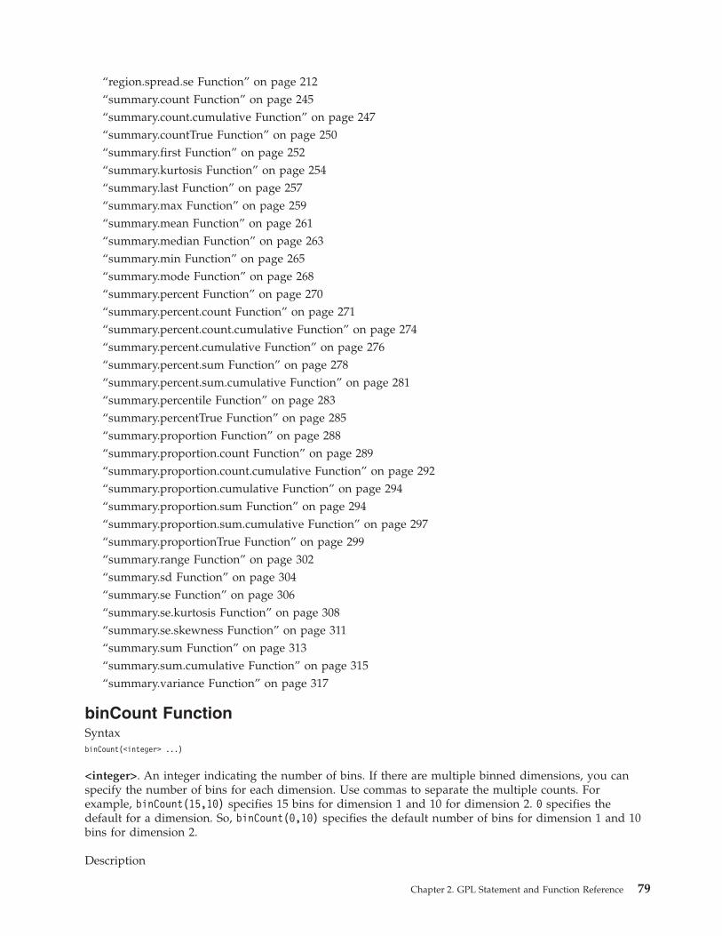
“region.spread.se Function” on page 212“summary.count Function” on page 245“summary.count.cumulative Function” on page 247“summary.countTrue Function” on page 250“summary.first Function” on page 252“summary.kurtosis Function” on page 254“summary.last Function” on page 257“summary.max Function” on page 259“summary.mean Function” on page 261“summary.median Function” on page 263“summary.min Function” on page 265“summary.mode Function” on page 268“summary.percent Function” on page 270“summary.percent.count Function” on page 271“summary.percent.count.cumulative Function” on page 274“summary.percent.cumulative Function” on page 276“summary.percent.sum Function” on page 278“summary.percent.sum.cumulative Function” on page 281“summary.percentile Function” on page 283“summary.percentTrue Function” on page 285“summary.proportion Function” on page 288“summary.proportion.count Function” on page 289“summary.proportion.count.cumulative Function” on page 292“summary.proportion.cumulative Function” on page 294“summary.proportion.sum Function” on page 294“summary.proportion.sum.cumulative Function” on page 297“summary.proportionTrue Function” on page 299“summary.range Function” on page 302“summary.sd Function” on page 304“summary.se Function” on page 306“summary.se.kurtosis Function” on page 308“summary.se.skewness Function” on page 311“summary.sum Function” on page 313“summary.sum.cumulative Function” on page 315“summary.variance Function” on page 317

binCount FunctionSyntaxbinCount(<integer> ...)

<integer>. An integer indicating the number of bins. If there are multiple binned dimensions, you canspecify the number of bins for each dimension. Use commas to separate the multiple counts. Forexample, binCount(15,10) specifies 15 bins for dimension 1 and 10 for dimension 2. 0 specifies thedefault for a dimension. So, binCount(0,10) specifies the default number of bins for dimension 1 and 10bins for dimension 2.

Description


Specifies the number of bins.

Examples

Applies To

“bin.dot Function” on page 70“bin.hex Function” on page 72“bin.rect Function” on page 77

binStart FunctionSyntaxbinStart(<value> ...)

<value>. An integer or quoted date literal indicating the value of the first bin. If there are multiplebinned dimensions, you can specify the first bin for each dimension. Use commas to separate themultiple first bins. For example, binStart(0,10) specifies 0 as the first bin on dimension 1 and 10 as thefirst bin on dimension 2. If you specify a value for one dimension, you have to specify a value for alldimensions.

Description

Specifies the value of the first bin. You can use the function to make sure bins begin at a specified value,regardless of the data values. Note that the first bin may not be drawn if there are no actual data valuesin that bin. However, the bin is still included when determining the number of bins and their widths.

If the specified value is greater than the lowest data value on the dimension, this function does not reallyspecify the starting value of the first bin because the function can never exclude smaller values from thebins. Rather, the function specifies the starting value for some other bin, depending on the width ornumber of bins. There may be one or more bins that precede the specified value.

Examples

Applies To


ELEMENT: interval(position(summary.count(bin.rect(salary, binCount(25)))))

Figure 110. Example: Defining a specific number of bins

ELEMENT: interval(position(bin.rect(salbegin*salary, dim(1,2), binCount(25,25))))

Figure 111. Example: Defining a specific number of bins for multiple binned dimensions

ELEMENT: interval(position(summary.count(bin.rect(salary, binStart(10000)))))

Figure 112. Example: Specifying the first bin on a continuous scale

ELEMENT: interval(position(summary.count(bin.rect(saledate, binStart("01/20/2003")))))

Figure 113. Example: Specifying the first bin on a date scale

ELEMENT: interval(position(bin.rect(x*y, dim(1,2), binStart(2000,1000))))

Figure 114. Example: Specifying the first bin for multiple binned dimensions


binWidth FunctionSyntaxbinWidth(<numeric> ...)

<numeric>. A positive numeric value indicating the width of the bins. If the data being binned are dates,the value indicates days or seconds, depending on the underlying data. To specify an explicit unit,append d or s to the value to indicate days or seconds, respectively. If there are multiple binneddimensions, you can specify the bin width for each dimension. Use commas to separate the multiplewidths. For example, binWidth(100,200) specifies 100 as the bin width for dimension 1 and 200 as thebin width for dimension 2. 0 specifies the default for a dimension. So, binWidth(0,200) specifies thedefault bin width for dimension 1 and 200 as the bin width for dimension 2.

Description

Specifies the width of the bins.

Examples

Applies To


chiSquare FunctionSyntaxchiSquare(<degrees of freedom>)

<degrees of freedom>. Numeric value specifying the degrees of freedom parameter for the distribution.This value must be greater than 0.

Description

Specifies a chi-square distribution for the probability scale.

ExamplesSCALE: prob(dim(2), chiSquare(5))

Applies To


closed FunctionSyntaxclosed()

Description

ELEMENT: interval(position(summary.count(bin.rect(salary, binWidth(1000)))))

Figure 115. Example: Defining a specific bin width

ELEMENT: interval(position(bin.rect(salbegin*salary, dim(1,2), binWidth(1000,2000))))

Figure 116. Example: Defining a specific bin width for multiple binned dimensions

ELEMENT: interval(position(summary.count(bin.rect(date, binWidth(30d)))))

Figure 117. Example: Defining a specific bin width for date data


Specifies that the end point of a graphic element is connected to its start point. In polar coordinates, thisresults in a closed loop around the center of the coordinate system.

Examples

Applies To


cluster FunctionSyntaxcluster(<integer> ...)

<integer>. One or more integers indicating the variable or variables in the algebra along whose axis theclustering occurs.

Description

Clusters graphic elements along a specific axis. You can also cluster graphic elements on more than oneaxis in 3-D charts.

Examples

In this example, jobcat is clustered in gender. Compare the position of the numbers in dim() to thepositions of the numbers in cluster(). In this case, the 1 in dim and 3 in cluster are the first numbers intheir respective functions. Therefore, clustering occurs on dim(3) (gender), and dim(1) (jobcat) specifies thevariable that defines the graphic elements in each cluster. If you removed the cluster function, the chartwould look similar, but dim(3) would specify a paneling facet and dim(1) would be the x axis. Theclustering collapses multiple panels into one, changing the way dimensions are displayed. For example,compare the following graphs.SOURCE: s = csvSource(file("Employee data.csv"))DATA: jobcat=col(source(s), name("jobcat"), unit.category())DATA: gender=col(source(s), name("gender"), unit.category())DATA: salary=col(source(s), name("salary"))COORD: rect(dim(1,2), cluster(3))SCALE: linear(dim(2), include(0))GUIDE: axis(dim(2), label("Mean Salary"))GUIDE: axis(dim(3), label("Gender"))ELEMENT: interval(position(summary.mean(jobcat*salary*gender)), color(jobcat))


ELEMENT: line(position(x*y), closed())

Figure 118. Example: Creating a closed line

COORD: rect(dim(1,2), cluster(3))ELEMENT: interval(position(summary.mean(jobcat*salary*gender)), color(jobcat))

Figure 119. Example: Clustering on the first dimension in a 2-D coordinate system


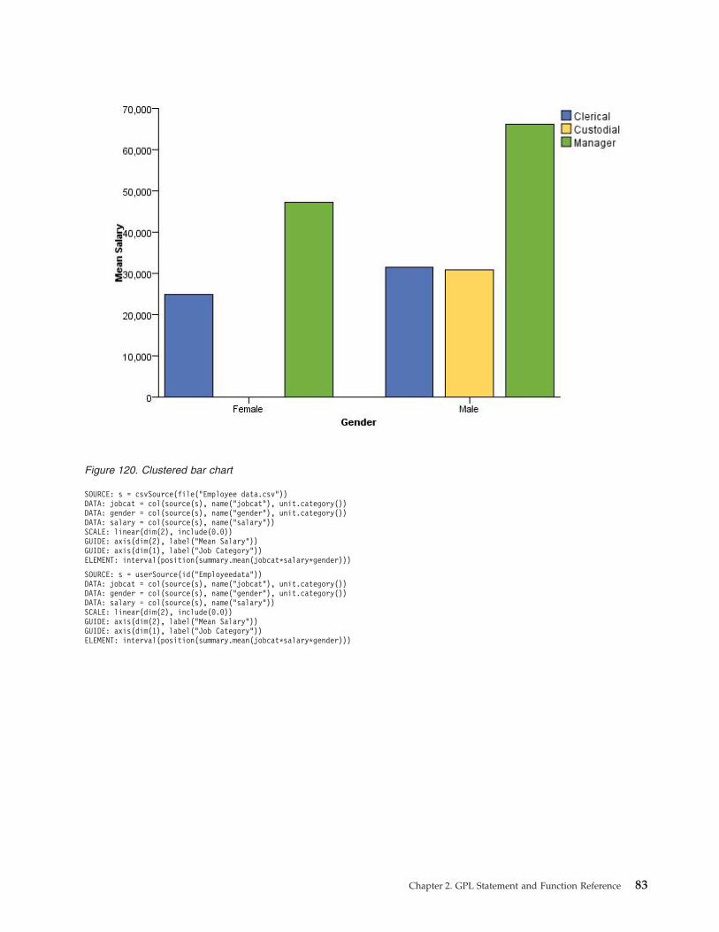
SOURCE: s = csvSource(file("Employee data.csv"))DATA: jobcat = col(source(s), name("jobcat"), unit.category())DATA: gender = col(source(s), name("gender"), unit.category())DATA: salary = col(source(s), name("salary"))SCALE: linear(dim(2), include(0.0))GUIDE: axis(dim(2), label("Mean Salary"))GUIDE: axis(dim(1), label("Job Category"))ELEMENT: interval(position(summary.mean(jobcat*salary*gender)))

SOURCE: s = userSource(id("Employeedata"))DATA: jobcat = col(source(s), name("jobcat"), unit.category())DATA: gender = col(source(s), name("gender"), unit.category())DATA: salary = col(source(s), name("salary"))SCALE: linear(dim(2), include(0.0))GUIDE: axis(dim(2), label("Mean Salary"))GUIDE: axis(dim(1), label("Job Category"))ELEMENT: interval(position(summary.mean(jobcat*salary*gender)))



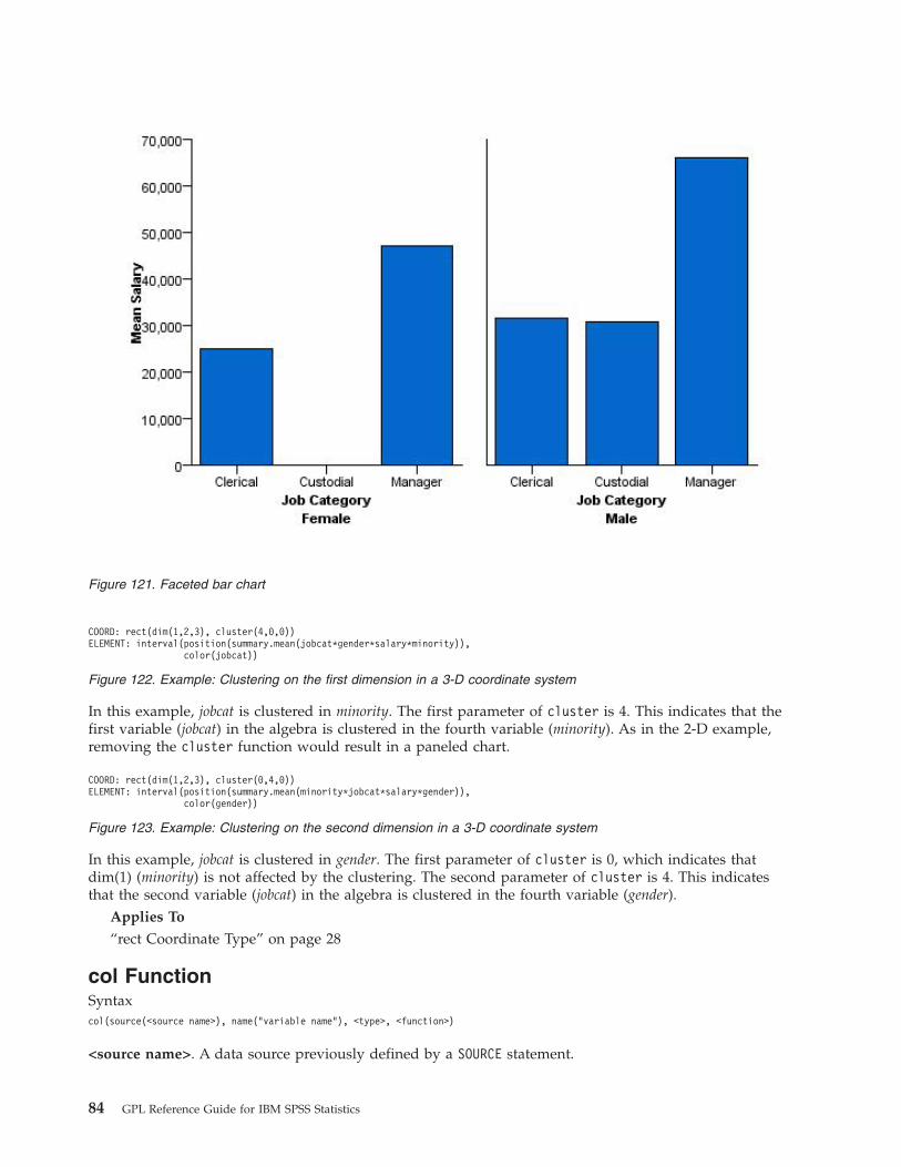
In this example, jobcat is clustered in minority. The first parameter of cluster is 4. This indicates that thefirst variable (jobcat) in the algebra is clustered in the fourth variable (minority). As in the 2-D example,removing the cluster function would result in a paneled chart.

In this example, jobcat is clustered in gender. The first parameter of cluster is 0, which indicates thatdim(1) (minority) is not affected by the clustering. The second parameter of cluster is 4. This indicatesthat the second variable (jobcat) in the algebra is clustered in the fourth variable (gender).

Applies To

“rect Coordinate Type” on page 28

col FunctionSyntaxcol(source(<source name>), name("variable name"), <type>, <function>)

<source name>. A data source previously defined by a SOURCE statement.


COORD: rect(dim(1,2,3), cluster(4,0,0))ELEMENT: interval(position(summary.mean(jobcat*gender*salary*minority)),

color(jobcat))

Figure 122. Example: Clustering on the first dimension in a 3-D coordinate system

COORD: rect(dim(1,2,3), cluster(0,4,0))ELEMENT: interval(position(summary.mean(minority*jobcat*salary*gender)),

color(gender))

Figure 123. Example: Clustering on the second dimension in a 3-D coordinate system


"variable name". The name of the variable in the data source.

<type>. A data type or measurement level. If no type is specified, the variable is assumed to becontinuous.


Description

Extracts a column of data from a data source. This is used for creating variables from the data.

Examples

Valid Types

unit.category. Specifies a categorical variable.

unit.time. Specifies a date variable. You will often need to specify the date format if using this type. Note:In IBM® SPSS® Statistics, dates from a userSource are passed to GPL as numeric values and are specifiedas continuous variables. Therefore, you should not use this type with a userSource.See the topic “formatFunction” on page 131 for more information.

Valid Functions

“in Function” on page 135“format Function” on page 131“notIn Function” on page 190Applies To

“DATA Statement” on page 24

collapse FunctionSyntaxcollapse(category(<algebra>), minimumPercent(<numeric>), sumVariable(<algebra>),

otherValue("label"))

<algebra>. Graph algebra, although in this case, the algebra should identify only one variable. Thevariable in category() identifies the variable whose categories are collapsed. The variable insumVariable() identifies the variable whose sum for the total compared to the sum for a particularcategory determines whether the category is collapsed.

<numeric>. A numeric value between 0 and 100 indicating a percentage. A category is collapsed if itssum is less than the specified percentage of the total sum for sumVariable.

"label". The label for the new variable containing the collapsed categories. This is the text that identifiesthe variable in the graph.

Description

DATA: age = col(source(mydata), name("age"))

Figure 124. Example: Specifying a continuous variable from a data source

DATA: gender = col(source(mydata), name("gender"), unit.category())

Figure 125. Example: Specifying a categorical variable from a data source

DATA: date = col(source(mydata), name("date"), unit.time(), format("M/d/yyyy"))

Figure 126. Example: Specifying a date variable from a data source


Collapse small categories of a categorical variable to create a new categorical variable. The functioncollapses the categories by recoding them to the value specified by otherValue.

Examples

Applies To

“TRANS Statement” on page 24

color Function (For GPL Graphic Elements)Note: If you are modifying the color for a guide, refer to “color Function (For GPL Guides)” on page 87.

Syntaxcolor(<algebra>)

orcolor(color.<color constant>)

orcolor(color."color value")

orcolor(<statistic function>)

<algebra>. Graph algebra, using one variable or a blend of variables. Each unique variable value resultsin a different color. For example, if you were creating a stacked bar chart, the argument of the colorfunction would be the variable that controls the stacking. Each stack segment would be a different color.

<color constant>. A constant indicating a specific color, such as red. See the topic “Color Constants” onpage 413 for more information. Color constants can also be blended (for example, color.blue+color.red).

"color value". A specific value that indicates the hexadecimal RGB color components (for example,color."6666FF").


Description

Controls the color of the graphic elements. To specify the color explicitly for the fill or border of thegraphic element, you can append .interior or .exterior to the function. Using color without a qualifierimplies color.interior.

Examples

TRANS: educ_collapse = collapse(category(educ), minimumPercent(10), sumVariable(salary),otherValue("Other"))

ELEMENT: interval(position(summary.sum(educ_collapse*salary))))

Figure 127. Example: Collapsing categories whose sum is less than 10% of total

ELEMENT: line(position(x*y), color(color.red))

Figure 128. Example: Specifying a color value with a constant

ELEMENT: line(position(x*y), color(color."FF0000"))

Figure 129. Example: Specifying a color value with RGB color components


Statistic Functions

See “GPL Functions” on page 56.Applies To

“area Element” on page 47“edge Element” on page 48“interval Element” on page 49“line Element” on page 49“path Element” on page 50“point Element” on page 51“polygon Element” on page 52“schema Element” on page 53

color Function (For GPL Guides)Note: If you are modifying the color for a graphic element (like a bar or point), refer to “color Function(For GPL Graphic Elements)” on page 86.

Syntaxcolor(color.<color constant>)

orcolor(color."color value")

<color constant>. A constant indicating a specific color, such as red. See the topic “Color Constants” onpage 413 for more information.

"color value". A specific value that indicates the hexadecimal RGB color components (for example,color."6666FF").

Description

Controls the color of guides, such as axes and reference lines.

Examples

Applies To

“axis Guide Type” on page 42“form.line Guide Type” on page 43

ELEMENT: interval(position(x*y), color.exterior(color.red))

Figure 130. Example: Specifying a color value for the bar border

ELEMENT: point(position(x*y), color(z))

Figure 131. Example: Using the values of a variable to control color

ELEMENT: interval(position(summary.mean(jobcat*salary)),color(summary.count()))

Figure 132. Example: Using a statistical function to control color

GUIDE: axis(dim(2), color(color.blue))

Figure 133. Example: Specifying an axis color


color.brightness Function (For GPL Graphic Elements)Note: If you are modifying the brightness for a guide, refer to “color.brightness Function (For GPLGuides)”.

Syntaxcolor.brightness(<algebra>)

orcolor.brightness(color.brightness."brightness value")

orcolor.brightness(<statistic function>)

<algebra>. Graph algebra, using one variable or a blend of variables. Each variable value results in adifferent level of color brightness.

"brightness value". A value between 0 and 1 that indicates the level of brightness. A value of 1 indicatesfull brightness, while a value of 0 indicates no brightness (black).


Description

Controls the color brightness of the graphic elements. To specify the color brightness explicitly for the fillor border of the graphic element, you can append .interior or .exterior to the function. Usingcolor.brightness without a qualifier implies color.brightness.interior.

Examples

Statistic Functions



color.brightness Function (For GPL Guides)Note: If you are modifying the brightness for a graphic element (like a bar or point), refer to“color.brightness Function (For GPL Graphic Elements)”.

ELEMENT: point(position(x*y), color.brightness(z), color(color.blue))

Figure 134. Example: Using the values of a variable to control color brightness

ELEMENT: interval(position(summary.mean(jobcat*salary)),color.brightness(summary.count()))

Figure 135. Example: Using a statistical function to control color brightness


Syntaxcolor.brightness(color.brightness."brightness value")

"brightness value". A value between 0 and 1 that indicates the level of brightness. A value of 1 indicatesfull brightness, while a value of 0 indicates no brightness (black).

Description

Controls the brightness of reference lines.

Examples

Applies To

“form.line Guide Type” on page 43

color.hue Function (For GPL Graphic Elements)Note: If you are modifying the hue for a guide, refer to “color.hue Function (For GPL Guides)” on page90.

Syntaxcolor.hue(<algebra>)

orcolor.hue(color.hue."hue value")

orcolor.hue(<statistic function>)

<algebra>. Graph algebra, using one variable or a blend of variables. Each variable value results in adifferent color hue.

"hue value". A value between 0 and 1 that indicates the hue level.


Description

Controls the color hue of the graphic elements. To specify the color hue explicitly for the fill or border ofthe graphic element, you can append .interior or .exterior to the function. Using color.hue without aqualifier implies color.hue.interior.

color.hue requires a base color other than white or black. Use color.interior or color.exterior to setthe base color.

Examples

GUIDE: form.line(position(*,2000), color.brightness(color.brightness."0.5"))

Figure 136. Example: Specifying a reference line brightness

ELEMENT: point(position(x*y), color.hue(z), color(color.blue))

Figure 137. Example: Using the values of a variable to control color hue


Statistic Functions



color.hue Function (For GPL Guides)Note: If you are modifying the hue for a graphic element (like a bar or point), refer to “color.hue Function(For GPL Graphic Elements)” on page 89.

Syntaxcolor.hue(color.brightness."hue value")

"hue value". A value between 0 and 1 that indicates the hue level.

Description

Controls the hue of reference lines.

Examples

Applies To


color.saturation Function (For GPL Graphic Elements)Note: If you are modifying the saturation for a guide, refer to “color.saturation Function (For GPLGuides)” on page 91.

Syntaxcolor.saturation(<algebra>)

orcolor.saturation(color.saturation."saturation value")

orcolor.saturation(<statistic function>)

<algebra>. Graph algebra, using one variable or a blend of variables. Each variable value results in adifferent level of color saturation.

ELEMENT: interval(position(summary.mean(jobcat*salary)),color.hue(summary.count()))

Figure 138. Example: Using a statistical function to control color hue

GUIDE: form.line(position(*,2000), color.hue(color.hue."0.5"))

Figure 139. Example: Specifying a reference line hue


"saturation value". A value between 0 and 1 that indicates the saturation level. A value of 1 indicates fullsaturation, while a value of 0 indicates no saturation (gray).


Description

Controls the color saturation of the graphic elements. To specify the color saturation explicitly for the fillor border of the graphic element, you can append .interior or .exterior to the function. Usingcolor.saturation without a qualifier implies color.saturation.interior.

Examples

Statistic Functions



color.saturation Function (For GPL Guides)Note: If you are modifying the saturation for a graphic element (like a bar or point), refer to“color.saturation Function (For GPL Graphic Elements)” on page 90.

Syntaxcolor.saturation(color.saturation."saturation value")

"saturation value". A value between 0 and 1 that indicates the saturation level. A value of 1 indicates fullsaturation, while a value of 0 indicates no saturation (gray).

Description

Controls the saturation of reference lines.

Examples

Applies To

ELEMENT: point(position(x*y), color.saturation(z), color(color.blue))

Figure 140. Example: Using the values of a variable to control color saturation

ELEMENT: interval(position(summary.mean(jobcat*salary)),color.saturation(summary.count()))

Figure 141. Example: Using a statistical function to control color

GUIDE: form.line(position(*,2000), color.saturation(color.saturation."0.5"))

Figure 142. Example: Specifying a reference line saturation



csvSource FunctionSyntaxcsvSource(file("file path"), key("key name"), <function>)

"file path". The path to the CSV file. This can be an absolute or relative path. The path is relative to thelocation of the application that parses the GPL code. Backslashes must be escaped with another backslash.You can also use forward slashes.

"key name". The name of a variable in the file that acts as a key. The key is used to link multiple sources,especially a dataset and a map file.


Description

Reads the contents of a comma-separated values (CSV) file. This function is used to assign the contents ofthe file to a data source.

Examples

Valid Functions

“missing.listwise Function” on page 187“missing.pairwise Function” on page 188“weight Function” on page 326Applies To

“SOURCE Statement” on page 23

dataMaximum FunctionSyntaxdataMaximum()

Description

Specifies that the maximum of the scale is exactly the same as the maximum of the data. Otherwise, a"nice" maximum is used. For example, if the last data value is 97, a "nice" maximum for the scale may be100. dataMaximum forces the scale to end at 97.

Examples

Applies To

“cLoglog Scale” on page 32“linear Scale” on page 34“log Scale” on page 34“pow Scale” on page 36

SOURCE: mydata = csvSource(file("/Data/Employee data.csv"))

Figure 143. Example: Reading a CSV file

SCALE: linear(dim(2), dataMaximum())

Figure 144. Example: Specifying a maximum on the 2nd dimension (y axis)



dataMinimum FunctionSyntaxdataMinimum()

Description

Specifies that minimum of the scale is exactly the same as the minimum of the data. Otherwise, a "nice"minimum is used. For example, if the first data value is 2, a "nice" minimum for the scale may be 0.dataMinimum forces the scale to begin at 2.

Examples

Applies To

“cLoglog Scale” on page 32“linear Scale” on page 34“log Scale” on page 34“pow Scale” on page 36“safeLog Scale” on page 38“safePower Scale” on page 39“time Scale” on page 40

delta FunctionSyntaxdelta(<numeric>)

<numeric>. A positive numeric value indicating the difference between major ticks on the axis. If theunderlying data along the axis are dates, the value indicates days.

Description

Specifies the difference between major ticks on an axis. Major ticks are the location at which labels aredisplayed along the axis.

Examples

Applies To

“axis Guide Type” on page 42

density.beta FunctionSyntaxdensity.beta(<algebra>, shape1(<numeric>), shape2(<numeric>), <function>)

SCALE: linear(dim(2), dataMinimum())

Figure 145. Example: Specifying a minimum on the 2nd dimension (y axis)

GUIDE: axis(dim(1), delta(1000))

Figure 146. Example: Specifying the distance between major ticks


ordensity.beta(<binning function>, shape1(<numeric>), shape2(<numeric>, <function>))

<algebra>. Graph algebra, such as x*y. Refer to “Brief Overview of GPL Algebra” on page 3 for anintroduction to graph algebra. The algebra is optional.

<binning function>. A binning function. The binning function is optional.

<numeric>. shape1 and shape2 define the parameters for the distribution. These take numeric values andare required.

<function>. A valid function. Use scaledToData("false") when comparing densities with very differentsame sizes.

Description

Calculates the probability density for the beta distribution. This is often used to add a distribution curve.The distribution is defined on the closed interval [0, 1]. If you don't see the graphic element for thedistribution, check the parameters for the distribution and the range for the x axis scale.

Because this function does not estimate parameters from the data, it can be used only for comparison andnot for fitting.

Examples

Binning Functions

“bin.dot Function” on page 70“bin.hex Function” on page 72“bin.quantile.letter Function” on page 75“bin.rect Function” on page 77Valid Functions

“scaledToData Function” on page 218Applies To

“bin.dot Function” on page 70“bin.hex Function” on page 72“bin.quantile.letter Function” on page 75“bin.rect Function” on page 77“color Function (For GPL Graphic Elements)” on page 86“color.brightness Function (For GPL Graphic Elements)” on page 88“color.hue Function (For GPL Graphic Elements)” on page 89“color.saturation Function (For GPL Graphic Elements)” on page 90“link.alpha Function” on page 154“link.complete Function” on page 156“link.delaunay Function” on page 159“link.distance Function” on page 161“link.gabriel Function” on page 163“link.hull Function” on page 165

ELEMENT: line(position(density.beta(x, shape1(2), shape2(5))))

Figure 147. Example: Adding a beta distribution curve


“link.influence Function” on page 168“link.join Function” on page 170“link.mst Function” on page 172“link.neighbor Function” on page 175“link.relativeNeighborhood Function” on page 177“link.sequence Function” on page 179“link.tsp Function” on page 181“position Function (For GPL Graphic Elements)” on page 192“region.confi.count Function” on page 196“region.confi.mean Function” on page 198“region.confi.percent.count Function” on page 200“region.confi.proportion.count Function” on page 202“region.confi.smooth Function” on page 205“region.spread.range Function” on page 207“region.spread.sd Function” on page 209“region.spread.se Function” on page 212“size Function (For GPL Graphic Elements)” on page 221“split Function” on page 243“summary.count Function” on page 245“summary.count.cumulative Function” on page 247“summary.countTrue Function” on page 250“summary.first Function” on page 252“summary.kurtosis Function” on page 254“summary.last Function” on page 257“summary.max Function” on page 259“summary.mean Function” on page 261“summary.median Function” on page 263“summary.min Function” on page 265“summary.mode Function” on page 268“summary.percent Function” on page 270“summary.percent.count Function” on page 271“summary.percent.count.cumulative Function” on page 274“summary.percent.cumulative Function” on page 276“summary.percent.sum Function” on page 278“summary.percent.sum.cumulative Function” on page 281“summary.percentile Function” on page 283“summary.percentTrue Function” on page 285“summary.proportion Function” on page 288“summary.proportion.count Function” on page 289“summary.proportion.count.cumulative Function” on page 292“summary.proportion.cumulative Function” on page 294“summary.proportion.sum Function” on page 294“summary.proportion.sum.cumulative Function” on page 297“summary.proportionTrue Function” on page 299“summary.range Function” on page 302


“summary.sd Function” on page 304“summary.se Function” on page 306“summary.se.kurtosis Function” on page 308“summary.se.skewness Function” on page 311“summary.sum Function” on page 313“summary.sum.cumulative Function” on page 315“summary.variance Function” on page 317“transparency Function (For GPL Graphic Elements)” on page 322

density.chiSquare FunctionSyntaxdensity.chiSquare(<algebra>, degreesOfFreedom(<integer>), <function>)

ordensity.chiSquare(<binning function>, degreesOfFreedom(<integer>), <function>)



<integer>. degreesOfFreedom defines the parameter for the distribution. This takes a positive integer andis required.


Description

Calculates the probability density of the chi-square distribution. This is often used to add a distributioncurve. If you don't see the graphic element for the distribution, check the parameter for the distributionand the range for the x axis scale.


Examples

Binning Functions



“bin.dot Function” on page 70“bin.hex Function” on page 72

ELEMENT: line(position(density.chiSquare(x, degreesoffreedom(5))))

Figure 148. Example: Adding a chi-square distribution curve


“bin.quantile.letter Function” on page 75“bin.rect Function” on page 77“color Function (For GPL Graphic Elements)” on page 86“color.brightness Function (For GPL Graphic Elements)” on page 88“color.hue Function (For GPL Graphic Elements)” on page 89“color.saturation Function (For GPL Graphic Elements)” on page 90“link.alpha Function” on page 154“link.complete Function” on page 156“link.delaunay Function” on page 159“link.distance Function” on page 161“link.gabriel Function” on page 163“link.hull Function” on page 165“link.influence Function” on page 168“link.join Function” on page 170“link.mst Function” on page 172“link.neighbor Function” on page 175“link.relativeNeighborhood Function” on page 177“link.sequence Function” on page 179“link.tsp Function” on page 181“position Function (For GPL Graphic Elements)” on page 192“region.confi.count Function” on page 196“region.confi.mean Function” on page 198“region.confi.percent.count Function” on page 200“region.confi.proportion.count Function” on page 202“region.confi.smooth Function” on page 205“region.spread.range Function” on page 207“region.spread.sd Function” on page 209“region.spread.se Function” on page 212“size Function (For GPL Graphic Elements)” on page 221“split Function” on page 243“summary.count Function” on page 245“summary.count.cumulative Function” on page 247“summary.countTrue Function” on page 250“summary.first Function” on page 252“summary.kurtosis Function” on page 254“summary.last Function” on page 257“summary.max Function” on page 259“summary.mean Function” on page 261“summary.median Function” on page 263“summary.min Function” on page 265“summary.mode Function” on page 268“summary.percent Function” on page 270“summary.percent.count Function” on page 271“summary.percent.count.cumulative Function” on page 274“summary.percent.cumulative Function” on page 276


“summary.percent.sum Function” on page 278“summary.percent.sum.cumulative Function” on page 281“summary.percentile Function” on page 283“summary.percentTrue Function” on page 285“summary.proportion Function” on page 288“summary.proportion.count Function” on page 289“summary.proportion.count.cumulative Function” on page 292“summary.proportion.cumulative Function” on page 294“summary.proportion.sum Function” on page 294“summary.proportion.sum.cumulative Function” on page 297“summary.proportionTrue Function” on page 299“summary.range Function” on page 302“summary.sd Function” on page 304“summary.se Function” on page 306“summary.se.kurtosis Function” on page 308“summary.se.skewness Function” on page 311“summary.sum Function” on page 313“summary.sum.cumulative Function” on page 315“summary.variance Function” on page 317“transparency Function (For GPL Graphic Elements)” on page 322

density.exponential FunctionSyntaxdensity.exponential(<algebra>, rate(<numeric>), <function>)

ordensity.exponential(<binning function>, rate(<numeric>), <function>)



<numeric>. rate defines the parameter for the distribution. This takes a numeric value greater than orequal to 0 and is optional. If the parameter is not specified, it is calculated from the underlying data.


Description

Calculates the probability density of the exponential distribution. This is often used to add a distributioncurve. If you don't see the graphic element for the distribution, check the parameter for the distributionand the range for the x axis scale.

Examples

Binning Functions

ELEMENT: line(position(density.exponential(x, rate(1.5))))

Figure 149. Example: Adding a chi-square distribution curve




“bin.dot Function” on page 70“bin.hex Function” on page 72“bin.quantile.letter Function” on page 75“bin.rect Function” on page 77“color Function (For GPL Graphic Elements)” on page 86“color.brightness Function (For GPL Graphic Elements)” on page 88“color.hue Function (For GPL Graphic Elements)” on page 89“color.saturation Function (For GPL Graphic Elements)” on page 90“link.alpha Function” on page 154“link.complete Function” on page 156“link.delaunay Function” on page 159“link.distance Function” on page 161“link.gabriel Function” on page 163“link.hull Function” on page 165“link.influence Function” on page 168“link.join Function” on page 170“link.mst Function” on page 172“link.neighbor Function” on page 175“link.relativeNeighborhood Function” on page 177“link.sequence Function” on page 179“link.tsp Function” on page 181“position Function (For GPL Graphic Elements)” on page 192“region.confi.count Function” on page 196“region.confi.mean Function” on page 198“region.confi.percent.count Function” on page 200“region.confi.proportion.count Function” on page 202“region.confi.smooth Function” on page 205“region.spread.range Function” on page 207“region.spread.sd Function” on page 209“region.spread.se Function” on page 212“size Function (For GPL Graphic Elements)” on page 221“split Function” on page 243“summary.count Function” on page 245“summary.count.cumulative Function” on page 247“summary.countTrue Function” on page 250“summary.first Function” on page 252“summary.kurtosis Function” on page 254“summary.last Function” on page 257


“summary.max Function” on page 259“summary.mean Function” on page 261“summary.median Function” on page 263“summary.min Function” on page 265“summary.mode Function” on page 268“summary.percent Function” on page 270“summary.percent.count Function” on page 271“summary.percent.count.cumulative Function” on page 274“summary.percent.cumulative Function” on page 276“summary.percent.sum Function” on page 278“summary.percent.sum.cumulative Function” on page 281“summary.percentile Function” on page 283“summary.percentTrue Function” on page 285“summary.proportion Function” on page 288“summary.proportion.count Function” on page 289“summary.proportion.count.cumulative Function” on page 292“summary.proportion.cumulative Function” on page 294“summary.proportion.sum Function” on page 294“summary.proportion.sum.cumulative Function” on page 297“summary.proportionTrue Function” on page 299“summary.range Function” on page 302“summary.sd Function” on page 304“summary.se Function” on page 306“summary.se.kurtosis Function” on page 308“summary.se.skewness Function” on page 311“summary.sum Function” on page 313“summary.sum.cumulative Function” on page 315“summary.variance Function” on page 317“transparency Function (For GPL Graphic Elements)” on page 322

density.f FunctionSyntaxdensity.f(<algebra>, degreesOfFreedom1(<integer>), degreesOfFreedom2(<integer>), <function>)

ordensity.f(<binning function>, degreesOfFreedom1(<integer>), degreesOfFreedom2(<integer>), <function>)



<integer>. degreesOfFreedom1 and degreesOfFreedom2 define the parameters for the distribution. Thesetake positive integers and are required.



Description

Calculates the probability density of the F distribution. This is often used to add a distribution curve. Ifyou don't see the graphic element for the distribution, check the parameters for the distribution and therange for the x axis scale.


Examples

Binning Functions



“bin.dot Function” on page 70“bin.hex Function” on page 72“bin.quantile.letter Function” on page 75“bin.rect Function” on page 77“color Function (For GPL Graphic Elements)” on page 86“color.brightness Function (For GPL Graphic Elements)” on page 88“color.hue Function (For GPL Graphic Elements)” on page 89“color.saturation Function (For GPL Graphic Elements)” on page 90“link.alpha Function” on page 154“link.complete Function” on page 156“link.delaunay Function” on page 159“link.distance Function” on page 161“link.gabriel Function” on page 163“link.hull Function” on page 165“link.influence Function” on page 168“link.join Function” on page 170“link.mst Function” on page 172“link.neighbor Function” on page 175“link.relativeNeighborhood Function” on page 177“link.sequence Function” on page 179“link.tsp Function” on page 181“position Function (For GPL Graphic Elements)” on page 192“region.confi.count Function” on page 196“region.confi.mean Function” on page 198“region.confi.percent.count Function” on page 200“region.confi.proportion.count Function” on page 202

ELEMENT: line(position(density.f(x, degreesoffreedom1(5), degreesoffreedom2(2))))

Figure 150. Example: Adding an F distribution curve


“region.confi.smooth Function” on page 205“region.spread.range Function” on page 207“region.spread.sd Function” on page 209“region.spread.se Function” on page 212“size Function (For GPL Graphic Elements)” on page 221“split Function” on page 243“summary.count Function” on page 245“summary.count.cumulative Function” on page 247“summary.countTrue Function” on page 250“summary.first Function” on page 252“summary.kurtosis Function” on page 254“summary.last Function” on page 257“summary.max Function” on page 259“summary.mean Function” on page 261“summary.median Function” on page 263“summary.min Function” on page 265“summary.mode Function” on page 268“summary.percent Function” on page 270“summary.percent.count Function” on page 271“summary.percent.count.cumulative Function” on page 274“summary.percent.cumulative Function” on page 276“summary.percent.sum Function” on page 278“summary.percent.sum.cumulative Function” on page 281“summary.percentile Function” on page 283“summary.percentTrue Function” on page 285“summary.proportion Function” on page 288“summary.proportion.count Function” on page 289“summary.proportion.count.cumulative Function” on page 292“summary.proportion.cumulative Function” on page 294“summary.proportion.sum Function” on page 294“summary.proportion.sum.cumulative Function” on page 297“summary.proportionTrue Function” on page 299“summary.range Function” on page 302“summary.sd Function” on page 304“summary.se Function” on page 306“summary.se.kurtosis Function” on page 308“summary.se.skewness Function” on page 311“summary.sum Function” on page 313“summary.sum.cumulative Function” on page 315“summary.variance Function” on page 317“transparency Function (For GPL Graphic Elements)” on page 322

density.gamma FunctionSyntaxdensity.gamma(<algebra>, rate(<numeric>), <function>)


ordensity.gamma(<binning function>, rate(<numeric>), <function>)



<numeric>. rate defines the parameter for the distribution. This takes a positive numeric value and isrequired.


Description

Calculates the probability density of the gamma distribution. This is often used to add a distributioncurve. If you don't see the graphic element for the distribution, check the parameters for the distributionand the range for the x axis scale.


Examples

Binning Functions




ELEMENT: line(position(density.gamma(x, rate(2.5))))

Figure 151. Example: Adding a gamma distribution curve


“link.influence Function” on page 168“link.join Function” on page 170“link.mst Function” on page 172“link.neighbor Function” on page 175“link.relativeNeighborhood Function” on page 177“link.sequence Function” on page 179“link.tsp Function” on page 181“position Function (For GPL Graphic Elements)” on page 192“region.confi.count Function” on page 196“region.confi.mean Function” on page 198“region.confi.percent.count Function” on page 200“region.confi.proportion.count Function” on page 202“region.confi.smooth Function” on page 205“region.spread.range Function” on page 207“region.spread.sd Function” on page 209“region.spread.se Function” on page 212“size Function (For GPL Graphic Elements)” on page 221“split Function” on page 243“summary.count Function” on page 245“summary.count.cumulative Function” on page 247“summary.countTrue Function” on page 250“summary.first Function” on page 252“summary.kurtosis Function” on page 254“summary.last Function” on page 257“summary.max Function” on page 259“summary.mean Function” on page 261“summary.median Function” on page 263“summary.min Function” on page 265“summary.mode Function” on page 268“summary.percent Function” on page 270“summary.percent.count Function” on page 271“summary.percent.count.cumulative Function” on page 274“summary.percent.cumulative Function” on page 276“summary.percent.sum Function” on page 278“summary.percent.sum.cumulative Function” on page 281“summary.percentile Function” on page 283“summary.percentTrue Function” on page 285“summary.proportion Function” on page 288“summary.proportion.count Function” on page 289“summary.proportion.count.cumulative Function” on page 292“summary.proportion.cumulative Function” on page 294“summary.proportion.sum Function” on page 294“summary.proportion.sum.cumulative Function” on page 297“summary.proportionTrue Function” on page 299“summary.range Function” on page 302



density.kernel FunctionSyntaxdensity.kernel.<kernel function>(<algebra>, fixedWindow(<numeric>), <function>)

ordensity.kernel.<kernel function>(<algebra>, nearestNeighbor(<integer>), <function>)

ordensity.kernel.<kernel function>.joint(<algebra>, fixedWindow(<numeric>), <function>)

ordensity.kernel.<kernel function>.joint(<algebra>, nearestNeighbor(<integer>), <function>)

<kernel function>. A kernel function. This specifies how data are weighted by the density function,depending on how close the data are to the current point.


<numeric>. fixedWindow specifies the proportion of data points to include when calculating the smoothfunction. This takes a numeric value between 0 and 1 and is optional. You also have the option of usingthe nearestNeighbor function to calculate smoother's bandwidth.

<integer>. nearestNeighbor specifies the k number of nearest neighbors to includes when calculating thesmooth function. This takes a positive integer and is optional. You also have the option of using thefixedWindow function to calculate the smoother's bandwidth.

<function>. One or more valid functions. These are optional. Use scaledToData("false") whencomparing densities with very different same sizes.

joint. Used to create densities based on values in the first (x axis) and second (y axis) dimensions.Without the joint modifier, the density is based only on values in the first (x axis) dimension. You wouldtypically use the modifier for 3-D densities.

Description

Calculates the probability density using a nonparametric kernel function. This is often used to add adistribution curve that does not assume a particular model (like normal or Poisson). You can use thefixedWindow function or the nearestNeighbor function to specify the smoother's bandwidth. If you do notspecify an explicit bandwidth, the internal algorithm uses a fixed window whose size is determined bythe underlying data values and the specific kernel function.

Examples


Kernel Functions

uniform. All data receive equal weights.

epanechnikov. Data near the current point receive higher weights than extreme data receive. Thisfunction weights extreme points more than the triweight, biweight, and tricube kernels but less than theGaussian and Cauchy kernels.

biweight. Data far from the current point receive more weight than the triweight kernel allows but lessweight than the Epanechnikov kernel permits.

tricube. Data close to the current point receive higher weights than both the Epanechnikov and biweightkernels allow.

triweight. Data close to the current point receive higher weights than any other kernel allows. Extremecases get very little weight.

gaussian. Weights follow a normal distribution, resulting in higher weighting of extreme cases than theEpanechnikov, biweight, tricube, and triweight kernels.

cauchy. Extreme values receive more weight than the other kernels, with the exception of the uniformkernel, allow.

Valid Functions

“marron Function” on page 184“scaledToData Function” on page 218“segments Function” on page 219Applies To

“bin.dot Function” on page 70“bin.hex Function” on page 72“bin.quantile.letter Function” on page 75“bin.rect Function” on page 77“color Function (For GPL Graphic Elements)” on page 86“color.brightness Function (For GPL Graphic Elements)” on page 88“color.hue Function (For GPL Graphic Elements)” on page 89“color.saturation Function (For GPL Graphic Elements)” on page 90“link.alpha Function” on page 154“link.complete Function” on page 156“link.delaunay Function” on page 159

ELEMENT: line(position(density.kernel.epanechnikov(x)))

Figure 152. Example: Adding the default kernel distribution

ELEMENT: line(position(density.kernel.epanechnikov(x, fixedWindow(0.05))))

Figure 153. Example: Adding a kernel distribution using a fixed window

ELEMENT: line(position(density.kernel.epanechnikov(x, nearestNeighbor(100))))

Figure 154. Example: Adding a kernel distribution using k nearest neighbors

COORD: rect(dim(1,2,3))ELEMENT: interval(position(density.kernel.epanechnikov.joint(x*y)))

Figure 155. Example: Creating a 3-D graph showing kernel densities


“link.distance Function” on page 161“link.gabriel Function” on page 163“link.hull Function” on page 165“link.influence Function” on page 168“link.join Function” on page 170“link.mst Function” on page 172“link.neighbor Function” on page 175“link.relativeNeighborhood Function” on page 177“link.sequence Function” on page 179“link.tsp Function” on page 181“position Function (For GPL Graphic Elements)” on page 192“region.confi.count Function” on page 196“region.confi.mean Function” on page 198“region.confi.percent.count Function” on page 200“region.confi.proportion.count Function” on page 202“region.confi.smooth Function” on page 205“region.spread.range Function” on page 207“region.spread.sd Function” on page 209“region.spread.se Function” on page 212“size Function (For GPL Graphic Elements)” on page 221“split Function” on page 243“summary.count Function” on page 245“summary.count.cumulative Function” on page 247“summary.countTrue Function” on page 250“summary.first Function” on page 252“summary.kurtosis Function” on page 254“summary.last Function” on page 257“summary.max Function” on page 259“summary.mean Function” on page 261“summary.median Function” on page 263“summary.min Function” on page 265“summary.mode Function” on page 268“summary.percent Function” on page 270“summary.percent.count Function” on page 271“summary.percent.count.cumulative Function” on page 274“summary.percent.cumulative Function” on page 276“summary.percent.sum Function” on page 278“summary.percent.sum.cumulative Function” on page 281“summary.percentile Function” on page 283“summary.percentTrue Function” on page 285“summary.proportion Function” on page 288“summary.proportion.count Function” on page 289“summary.proportion.count.cumulative Function” on page 292“summary.proportion.cumulative Function” on page 294“summary.proportion.sum Function” on page 294


“summary.proportion.sum.cumulative Function” on page 297“summary.proportionTrue Function” on page 299“summary.range Function” on page 302“summary.sd Function” on page 304“summary.se Function” on page 306“summary.se.kurtosis Function” on page 308“summary.se.skewness Function” on page 311“summary.sum Function” on page 313“summary.sum.cumulative Function” on page 315“summary.variance Function” on page 317“transparency Function (For GPL Graphic Elements)” on page 322

density.logistic FunctionSyntaxdensity.logistic(<algebra>, location(<numeric>), scaleDensity(<numeric>), <function>)

ordensity.logistic(<binning function>, location(<numeric>), scaleDensity(<numeric>), <function>)



<integer>. location and scaleDensity define the parameters for the distribution. These take numericvalues and are required.


Description

Calculates the probability density of the logistic distribution. This is often used to add a distributioncurve. If you don't see the graphic element for the distribution, check the parameters for the distributionand the range for the x axis scale.


Examples

Binning Functions


“scaledToData Function” on page 218

ELEMENT: line(position(density.logistic(x, location(5), scaleDensity(2))))

Figure 156. Example: Adding a logistic distribution curve


Applies To

“bin.dot Function” on page 70“bin.hex Function” on page 72“bin.quantile.letter Function” on page 75“bin.rect Function” on page 77“color Function (For GPL Graphic Elements)” on page 86“color.brightness Function (For GPL Graphic Elements)” on page 88“color.hue Function (For GPL Graphic Elements)” on page 89“color.saturation Function (For GPL Graphic Elements)” on page 90“link.alpha Function” on page 154“link.complete Function” on page 156“link.delaunay Function” on page 159“link.distance Function” on page 161“link.gabriel Function” on page 163“link.hull Function” on page 165“link.influence Function” on page 168“link.join Function” on page 170“link.mst Function” on page 172“link.neighbor Function” on page 175“link.relativeNeighborhood Function” on page 177“link.sequence Function” on page 179“link.tsp Function” on page 181“position Function (For GPL Graphic Elements)” on page 192“region.confi.count Function” on page 196“region.confi.mean Function” on page 198“region.confi.percent.count Function” on page 200“region.confi.proportion.count Function” on page 202“region.confi.smooth Function” on page 205“region.spread.range Function” on page 207“region.spread.sd Function” on page 209“region.spread.se Function” on page 212“size Function (For GPL Graphic Elements)” on page 221“split Function” on page 243“summary.count Function” on page 245“summary.count.cumulative Function” on page 247“summary.countTrue Function” on page 250“summary.first Function” on page 252“summary.kurtosis Function” on page 254“summary.last Function” on page 257“summary.max Function” on page 259“summary.mean Function” on page 261“summary.median Function” on page 263“summary.min Function” on page 265“summary.mode Function” on page 268“summary.percent Function” on page 270


“summary.percent.count Function” on page 271“summary.percent.count.cumulative Function” on page 274“summary.percent.cumulative Function” on page 276“summary.percent.sum Function” on page 278“summary.percent.sum.cumulative Function” on page 281“summary.percentile Function” on page 283“summary.percentTrue Function” on page 285“summary.proportion Function” on page 288“summary.proportion.count Function” on page 289“summary.proportion.count.cumulative Function” on page 292“summary.proportion.cumulative Function” on page 294“summary.proportion.sum Function” on page 294“summary.proportion.sum.cumulative Function” on page 297“summary.proportionTrue Function” on page 299“summary.range Function” on page 302“summary.sd Function” on page 304“summary.se Function” on page 306“summary.se.kurtosis Function” on page 308“summary.se.skewness Function” on page 311“summary.sum Function” on page 313“summary.sum.cumulative Function” on page 315“summary.variance Function” on page 317“transparency Function (For GPL Graphic Elements)” on page 322

density.normal FunctionSyntaxdensity.normal(<algebra>, mean(<numeric>), standardDeviation(<numeric>), <function>)

ordensity.normal(<binning function>, mean(<numeric>), standardDeviation(<numeric>), <function>)



<numeric>. mean and standardDeviation define the parameters for the distribution. These take numericvalues. You can use both of them or neither. If no parameters are specified, they are calculated from theunderlying data.


Description

Calculates the probability density of the normal distribution. This is often used to add a distributioncurve.

Examples


Binning Functions



“bin.dot Function” on page 70“bin.hex Function” on page 72“bin.quantile.letter Function” on page 75“bin.rect Function” on page 77“color Function (For GPL Graphic Elements)” on page 86“color.brightness Function (For GPL Graphic Elements)” on page 88“color.hue Function (For GPL Graphic Elements)” on page 89“color.saturation Function (For GPL Graphic Elements)” on page 90“link.alpha Function” on page 154“link.complete Function” on page 156“link.delaunay Function” on page 159“link.distance Function” on page 161“link.gabriel Function” on page 163“link.hull Function” on page 165“link.influence Function” on page 168“link.join Function” on page 170“link.mst Function” on page 172“link.neighbor Function” on page 175“link.relativeNeighborhood Function” on page 177“link.sequence Function” on page 179“link.tsp Function” on page 181“position Function (For GPL Graphic Elements)” on page 192“region.confi.count Function” on page 196“region.confi.mean Function” on page 198“region.confi.percent.count Function” on page 200“region.confi.proportion.count Function” on page 202“region.confi.smooth Function” on page 205“region.spread.range Function” on page 207“region.spread.sd Function” on page 209“region.spread.se Function” on page 212“size Function (For GPL Graphic Elements)” on page 221

ELEMENT: interval(position(summary.count(bin.rect(x))))ELEMENT: line(position(density.normal(x)))

Figure 157. Example: Adding a normal curve to a histogram

ELEMENT: line(position(density.normal(x, mean(50000), standardDeviation(15000))))

Figure 158. Example: Creating a normal curve with specific parameters


“split Function” on page 243“summary.count Function” on page 245“summary.count.cumulative Function” on page 247“summary.countTrue Function” on page 250“summary.first Function” on page 252“summary.kurtosis Function” on page 254“summary.last Function” on page 257“summary.max Function” on page 259“summary.mean Function” on page 261“summary.median Function” on page 263“summary.min Function” on page 265“summary.mode Function” on page 268“summary.percent Function” on page 270“summary.percent.count Function” on page 271“summary.percent.count.cumulative Function” on page 274“summary.percent.cumulative Function” on page 276“summary.percent.sum Function” on page 278“summary.percent.sum.cumulative Function” on page 281“summary.percentile Function” on page 283“summary.percentTrue Function” on page 285“summary.proportion Function” on page 288“summary.proportion.count Function” on page 289“summary.proportion.count.cumulative Function” on page 292“summary.proportion.cumulative Function” on page 294“summary.proportion.sum Function” on page 294“summary.proportion.sum.cumulative Function” on page 297“summary.proportionTrue Function” on page 299“summary.range Function” on page 302“summary.sd Function” on page 304“summary.se Function” on page 306“summary.se.kurtosis Function” on page 308“summary.se.skewness Function” on page 311“summary.sum Function” on page 313“summary.sum.cumulative Function” on page 315“summary.variance Function” on page 317“transparency Function (For GPL Graphic Elements)” on page 322

density.poisson FunctionSyntaxdensity.poisson(<algebra>, rate(<numeric>), <function>)

ordensity.poisson(<binning function>, rate(<numeric>), <function>)




<numeric>. rate defines the parameter for the distribution. This takes a positive numeric value and isoptional. If the parameter is not specified, it is calculated from the underlying data.


Description

Calculates the probability density of the Poisson distribution. This is often used to add a distributioncurve. If you don't see the graphic element for the distribution, check the parameter for the distributionand the range for the x axis scale.

Examples

Binning Functions



“bin.dot Function” on page 70“bin.hex Function” on page 72“bin.quantile.letter Function” on page 75“bin.rect Function” on page 77“color Function (For GPL Graphic Elements)” on page 86“color.brightness Function (For GPL Graphic Elements)” on page 88“color.hue Function (For GPL Graphic Elements)” on page 89“color.saturation Function (For GPL Graphic Elements)” on page 90“link.alpha Function” on page 154“link.complete Function” on page 156“link.delaunay Function” on page 159“link.distance Function” on page 161“link.gabriel Function” on page 163“link.hull Function” on page 165“link.influence Function” on page 168“link.join Function” on page 170“link.mst Function” on page 172“link.neighbor Function” on page 175“link.relativeNeighborhood Function” on page 177“link.sequence Function” on page 179“link.tsp Function” on page 181“position Function (For GPL Graphic Elements)” on page 192

ELEMENT: line(position(density.poisson(x, rate(5.5))))

Figure 159. Example: Adding a Poisson distribution curve


“region.confi.count Function” on page 196“region.confi.mean Function” on page 198“region.confi.percent.count Function” on page 200“region.confi.proportion.count Function” on page 202“region.confi.smooth Function” on page 205“region.spread.range Function” on page 207“region.spread.sd Function” on page 209“region.spread.se Function” on page 212“size Function (For GPL Graphic Elements)” on page 221“split Function” on page 243“summary.count Function” on page 245“summary.count.cumulative Function” on page 247“summary.countTrue Function” on page 250“summary.first Function” on page 252“summary.kurtosis Function” on page 254“summary.last Function” on page 257“summary.max Function” on page 259“summary.mean Function” on page 261“summary.median Function” on page 263“summary.min Function” on page 265“summary.mode Function” on page 268“summary.percent Function” on page 270“summary.percent.count Function” on page 271“summary.percent.count.cumulative Function” on page 274“summary.percent.cumulative Function” on page 276“summary.percent.sum Function” on page 278“summary.percent.sum.cumulative Function” on page 281“summary.percentile Function” on page 283“summary.percentTrue Function” on page 285“summary.proportion Function” on page 288“summary.proportion.count Function” on page 289“summary.proportion.count.cumulative Function” on page 292“summary.proportion.cumulative Function” on page 294“summary.proportion.sum Function” on page 294“summary.proportion.sum.cumulative Function” on page 297“summary.proportionTrue Function” on page 299“summary.range Function” on page 302“summary.sd Function” on page 304“summary.se Function” on page 306“summary.se.kurtosis Function” on page 308“summary.se.skewness Function” on page 311“summary.sum Function” on page 313“summary.sum.cumulative Function” on page 315“summary.variance Function” on page 317“transparency Function (For GPL Graphic Elements)” on page 322


density.studentizedRange FunctionSyntaxdensity.studentizedRange(<algebra>, degreesOfFreedom(<integer>), k(<numeric>), <function>)

ordensity.studentizedRange(<binning function>, degreesOfFreedom(<integer>), k(<numeric>), <function>)



<integer> and <numeric>. degreesOfFreedom and k define the parameters for the distribution.degreesOfFreedom takes an integer, and k takes a numeric value. These are required.


Description

Calculates the probability density of the Studentized range distribution. This is often used to add adistribution curve. If you don't see the graphic element for the distribution, check the parameters for thedistribution and the range for the x axis scale.


Examples

Binning Functions




ELEMENT: line(position(density.studentizedRange(x, degreesOfFreedom(5), k(2.5))))

Figure 160. Example: Adding a Studentized range distribution curve





density.t FunctionSyntaxdensity.t(<algebra>, degreesOfFreedom(<integer>), <function>)

ordensity.t(<binning function>, degreesOfFreedom(<integer>), <function>)



<integer>. degreesOfFreedom defines the parameter for the distribution. degreesOfFreedom takes aninteger and is required.


Description

Calculates the probability density of the Student's t distribution. This is often used to add a distributioncurve. If you don't see the graphic element for the distribution, check the parameters for the distributionand the range for the x axis scale.


Examples

Binning Functions


“scaledToData Function” on page 218

ELEMENT: line(position(density.t(x, degreesOfFreedom(5))))

Figure 161. Example: Adding a Student's t distribution curve


Applies To




density.uniform FunctionSyntaxdensity.uniform(<algebra>, min(<numeric>), max(<numeric>), <function>)

ordensity.uniform(<binning function>, min(<numeric>), max(<numeric>), <function>)



<numeric>. min and max define the parameters for the distribution. These take numeric values. You canuse all of them or none of them. Any missing parameters are calculated from the underlying data.


Description

Calculates the probability density of the uniform distribution using the method-of-moments estimate.This is often used to add a distribution curve.

Examples


Binning Functions



“bin.dot Function” on page 70“bin.hex Function” on page 72“bin.quantile.letter Function” on page 75“bin.rect Function” on page 77“color Function (For GPL Graphic Elements)” on page 86“color.brightness Function (For GPL Graphic Elements)” on page 88“color.hue Function (For GPL Graphic Elements)” on page 89“color.saturation Function (For GPL Graphic Elements)” on page 90“link.alpha Function” on page 154“link.complete Function” on page 156“link.delaunay Function” on page 159“link.distance Function” on page 161“link.gabriel Function” on page 163“link.hull Function” on page 165“link.influence Function” on page 168“link.join Function” on page 170“link.mst Function” on page 172“link.neighbor Function” on page 175“link.relativeNeighborhood Function” on page 177“link.sequence Function” on page 179“link.tsp Function” on page 181“position Function (For GPL Graphic Elements)” on page 192“region.confi.count Function” on page 196“region.confi.mean Function” on page 198“region.confi.percent.count Function” on page 200“region.confi.proportion.count Function” on page 202“region.confi.smooth Function” on page 205“region.spread.range Function” on page 207“region.spread.sd Function” on page 209“region.spread.se Function” on page 212“size Function (For GPL Graphic Elements)” on page 221“split Function” on page 243“summary.count Function” on page 245“summary.count.cumulative Function” on page 247

ELEMENT: line(position(density.uniform(x)))

Figure 162. Example: Adding a uniform distribution curve


“summary.countTrue Function” on page 250“summary.first Function” on page 252“summary.kurtosis Function” on page 254“summary.last Function” on page 257“summary.max Function” on page 259“summary.mean Function” on page 261“summary.median Function” on page 263“summary.min Function” on page 265“summary.mode Function” on page 268“summary.percent Function” on page 270“summary.percent.count Function” on page 271“summary.percent.count.cumulative Function” on page 274“summary.percent.cumulative Function” on page 276“summary.percent.sum Function” on page 278“summary.percent.sum.cumulative Function” on page 281“summary.percentile Function” on page 283“summary.percentTrue Function” on page 285“summary.proportion Function” on page 288“summary.proportion.count Function” on page 289“summary.proportion.count.cumulative Function” on page 292“summary.proportion.cumulative Function” on page 294“summary.proportion.sum Function” on page 294“summary.proportion.sum.cumulative Function” on page 297“summary.proportionTrue Function” on page 299“summary.range Function” on page 302“summary.sd Function” on page 304“summary.se Function” on page 306“summary.se.kurtosis Function” on page 308“summary.se.skewness Function” on page 311“summary.sum Function” on page 313“summary.sum.cumulative Function” on page 315“summary.variance Function” on page 317“transparency Function (For GPL Graphic Elements)” on page 322

density.weibull FunctionSyntaxdensity.weibull(<algebra>, rate(<numeric>), scaleDensity(<numeric>), <function>)

ordensity.weibull(<binning function>, rate(<numeric>), scaleDensity(<numeric>), <function>)




<integer>. rate and scaleDensity define the parameters for the distribution. These take numeric valuesand are required.


Description

Calculates the probability density of the Weibull distribution. This is often used to add a distributioncurve. If you don't see the graphic element for the distribution, check the parameters for the distributionand the range for the x axis scale.


Examples

Binning Functions



“bin.dot Function” on page 70“bin.hex Function” on page 72“bin.quantile.letter Function” on page 75“bin.rect Function” on page 77“color Function (For GPL Graphic Elements)” on page 86“color.brightness Function (For GPL Graphic Elements)” on page 88“color.hue Function (For GPL Graphic Elements)” on page 89“color.saturation Function (For GPL Graphic Elements)” on page 90“link.alpha Function” on page 154“link.complete Function” on page 156“link.delaunay Function” on page 159“link.distance Function” on page 161“link.gabriel Function” on page 163“link.hull Function” on page 165“link.influence Function” on page 168“link.join Function” on page 170“link.mst Function” on page 172“link.neighbor Function” on page 175“link.relativeNeighborhood Function” on page 177“link.sequence Function” on page 179“link.tsp Function” on page 181

ELEMENT: line(position(density.logistic(x, location(5), scaleDensity(2))))

Figure 163. Example: Adding a Weibull distribution curve


“position Function (For GPL Graphic Elements)” on page 192“region.confi.count Function” on page 196“region.confi.mean Function” on page 198“region.confi.percent.count Function” on page 200“region.confi.proportion.count Function” on page 202“region.confi.smooth Function” on page 205“region.spread.range Function” on page 207“region.spread.sd Function” on page 209“region.spread.se Function” on page 212“size Function (For GPL Graphic Elements)” on page 221“split Function” on page 243“summary.count Function” on page 245“summary.count.cumulative Function” on page 247“summary.countTrue Function” on page 250“summary.first Function” on page 252“summary.kurtosis Function” on page 254“summary.last Function” on page 257“summary.max Function” on page 259“summary.mean Function” on page 261“summary.median Function” on page 263“summary.min Function” on page 265“summary.mode Function” on page 268“summary.percent Function” on page 270“summary.percent.count Function” on page 271“summary.percent.count.cumulative Function” on page 274“summary.percent.cumulative Function” on page 276“summary.percent.sum Function” on page 278“summary.percent.sum.cumulative Function” on page 281“summary.percentile Function” on page 283“summary.percentTrue Function” on page 285“summary.proportion Function” on page 288“summary.proportion.count Function” on page 289“summary.proportion.count.cumulative Function” on page 292“summary.proportion.cumulative Function” on page 294“summary.proportion.sum Function” on page 294“summary.proportion.sum.cumulative Function” on page 297“summary.proportionTrue Function” on page 299“summary.range Function” on page 302“summary.sd Function” on page 304“summary.se Function” on page 306“summary.se.kurtosis Function” on page 308“summary.se.skewness Function” on page 311“summary.sum Function” on page 313“summary.sum.cumulative Function” on page 315“summary.variance Function” on page 317


“transparency Function (For GPL Graphic Elements)” on page 322

dim FunctionSyntaxdim(<numeric> ...)

<numeric>. A numeric value identifying the dimension or dimensions. If you are specifying multipledimensions, use commas to separate the numeric values.

Description

Specifies the dimension or dimensions to which a coordinate type, scale, guide, or function applies.

To figure out the numeric value associated with a dimension, look at the algebra. Counting the crossingsgives the main dimension values. The coordinate system (including any clustering of the coordinatesystem) doesn't matter.

Consider the following algebra:a*b*c*d

The variables in the algebra correspond to the following dimensions:

Table 2. Variables and dimensions.

Variable Dimension

a dim(1)

b dim(2)

c dim(3)

d dim(4)

Blended variables cannot be separated. The blend of the two variables corresponds to one dimension.Consider the following:a*(b+c)*d


Table 3. Variables and dimensions with blended variables.

Variable Dimension

a dim(1)

b+c dim(2)

d dim(3)

With nesting, you still count crossed variables, but nested groups are counted only once. To refer to eachvariable in the nested group, you count from the outside in, using a dot convention. The outermostvariable in the nested group gets the primary dimension number (for example, dim(1)), and the nextvariable gets the primary dimension number followed by a dot and a 1 (for example, dim(1.1)). Considerthe following:a*b/c*d



Variable Dimension

a dim(1)

c dim(2)

b dim(2.1)

d dim(3)

Examples

Applies To

“base.coordinate Function” on page 68“bin.dot Function” on page 70“bin.hex Function” on page 72“bin.rect Function” on page 77“reflect Function” on page 195“parallel Coordinate Type” on page 26“polar Coordinate Type” on page 26“polar.theta Coordinate Type” on page 27“rect Coordinate Type” on page 28“axis Guide Type” on page 42“asn Scale” on page 30“atanh Scale” on page 31“cat Scale” on page 32“cLoglog Scale” on page 32“linear Scale” on page 34“log Scale” on page 34“logit Scale” on page 35“pow Scale” on page 36“prob Scale” on page 37“probit Scale” on page 37“safeLog Scale” on page 38“safePower Scale” on page 39“time Scale” on page 40

end Function

Syntaxend()

Description

Specifies the end of the GPL block that defines a particular graph or page.

COORD: rect(dim(1,2))

Figure 164. Example: Specifying a two-dimensional, rectangular coordinate system

GUIDE: axis(dim(2), label("Mean Salary"))

Figure 165. Example: Specifying an axis label for the second dimension


Examples

Applies To

“GRAPH Statement” on page 22“PAGE Statement” on page 22

eval FunctionSyntaxeval(<expression>)

<expression>. A mathematical expression, such as log(salary).

Description

Evaluates a mathematical expression for each case in the data. You can use many different mathematicalfunctions in the expression. See the topic “eval Operators and Functions” on page 127 for moreinformation. If needed, you can wrap the result of a function in another function. Therefore,datetostring(date()) is a valid expression.

The eval function is also useful for evaluating a Boolean expression whose result can be used in thesummary.countTrue, summary.percentTrue, and summary.proportionTrue functions. This combinationallows you to plot the number or percent of cases greater than or less than a specific value.

Examples

Applies To

“TRANS Statement” on page 24“collapse Function” on page 85

GRAPH: begin()ELEMENT: line(position(x*y))GRAPH: end()

Figure 166. Example: Defining a particular graph

PAGE: begin(scale(400px,300px))SOURCE: s=csvSource(file("mydata.csv"))DATA: x=col(source(s), name("x"))DATA: y=col(source(s), name("y"))ELEMENT: line(position(x*y))PAGE: end()

Figure 167. Example: Defining a page

TRANS: saldiff = eval(salary-salbegin)ELEMENT: point(position(summary.mean(jobcat*saldiff)))

Figure 168. Example: Plotting the difference between two variables

DATA: x = iter(-100,100,1)TRANS: y = eval(x**2)ELEMENT: line(position(x*y))

Figure 169. Example: Creating a graph from an equation

TRANS: salGreaterThan = eval(salary>50000)ELEMENT: interval(position(summary.percentTrue(jobcat*salGreaterThan)))

Figure 170. Example: Plotting percent greater than a value


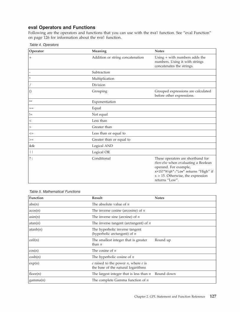
eval Operators and FunctionsFollowing are the operators and functions that you can use with the eval function. See “eval Function”on page 126 for information about the eval function.

Table 4. Operators

Operator Meaning Notes

+ Addition or string concatenation Using + with numbers adds thenumbers. Using it with stringsconcatenates the strings.

- Subtraction

* Multiplication

/ Division

() Grouping Grouped expressions are calculatedbefore other expressions.

** Exponentiation

== Equal

!= Not equal

< Less than

> Greater than

<= Less than or equal to

>= Greater than or equal to

&& Logical AND

|| Logical OR

? : Conditional These operators are shorthand forthen-else when evaluating a Booleanoperand. For example,x>15?”High”:”Low” returns “High” ifx > 15. Otherwise, the expressionreturns “Low”.

Table 5. Mathematical Functions

Function Result Notes

abs(n) The absolute value of n

acos(n) The inverse cosine (arcosine) of n

asin(n) The inverse sine (arcsine) of n

atan(n) The inverse tangent (arctangent) of n

atanh(n) The hyperbolic inverse tangent(hyperbolic arctangent) of n

ceil(n) The smallest integer that is greaterthan n

Round up

cos(n) The cosine of n

cosh(n) The hyperbolic cosine of n

exp(n) e raised to the power n, where e isthe base of the natural logarithms

floor(n) The largest integer that is less than n Round down

gamma(n) The complete Gamma function of n


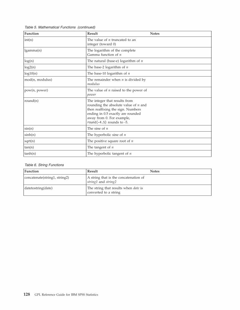
Table 5. Mathematical Functions (continued)


int(n) The value of n truncated to aninteger (toward 0)

lgamma(n) The logarithm of the completeGamma function of n

log(n) The natural (base-e) logarithm of n

log2(n) The base-2 logarithm of n

log10(n) The base-10 logarithm of n

mod(n, modulus) The remainder when n is divided bymodulus

pow(n, power) The value of n raised to the power ofpower

round(n) The integer that results fromrounding the absolute value of n andthen reaffixing the sign. Numbersending in 0.5 exactly are roundedaway from 0. For example,round(-4.5) rounds to -5.

sin(n) The sine of n

sinh(n) The hyperbolic sine of n

sqrt(n) The positive square root of n

tan(n) The tangent of n

tanh(n) The hyperbolic tangent of n

Table 6. String Functions


concatenate(string1, string2) A string that is the concatenation ofstring1 and string2

datetostring(date) The string that results when date isconverted to a string


Table 6. String Functions (continued)


indexof(haystack,needle[,divisor]) A number that indicates the positionof the first occurrence of needle inhaystack. The optional third argument,divisor, is a number of charactersused to divide needle into separatestrings. Each substring is used forsearching and the function returnsthe first occurrence of any of thesubstrings. For example, indexof(x,“abcd”) will return the value of thestarting position of the completestring "abcd" in the string variable x;indexof(x, “abcd”, 1) will return thevalue of the position of the firstoccurrence of any of the values in thestring; and indexof(x, “abcd”, 2) willreturn the value of the firstoccurrence of either "ab" or "cd".Divisor must be a positive integerand must divide evenly into thelength of needle. Returns 0 if needledoes not occur within haystack.

length(string) A number indicating the length ofstring

lowercase(string) string with uppercase letters changedto lowercase and other charactersunchanged

ltrim(string[, char]) string with any leading instances ofchar removed. If char is not specified,leading blanks are removed. Charmust resolve to a single character.

midstring(string , start, end) The substring beginning at positionstart of string and ending at end

numbertostring(n) The string that results when n isconverted to a string

replace(target, old, new) In target, instances of old are replacedwith new. All arguments are strings.

rtrim(string[, char]) string with any trailing instances ofchar removed. If char is not specified,trailing blanks are removed. Charmust resolve to a single character.

stringtodate(string) The value of the string expressionstring as a date

stringtonumber(string) The value of the string expressionstring as a number

substring(string, start, length) The substring beginning at positionstart of string and running for lengthlength

trim(string) string with any leading and trailingblanks removed


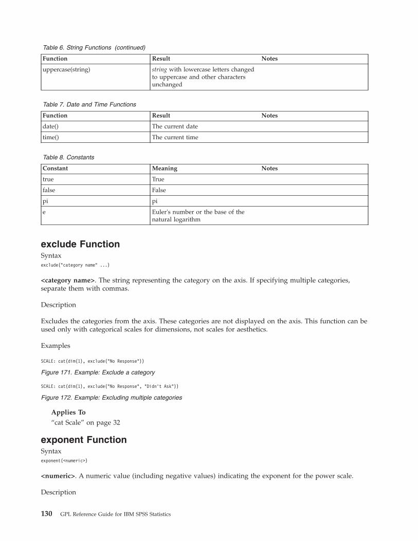
Table 6. String Functions (continued)


uppercase(string) string with lowercase letters changedto uppercase and other charactersunchanged

Table 7. Date and Time Functions


date() The current date

time() The current time

Table 8. Constants

Constant Meaning Notes

true True

false False

pi pi

e Euler's number or the base of thenatural logarithm

exclude FunctionSyntaxexclude("category name" ...)

<category name>. The string representing the category on the axis. If specifying multiple categories,separate them with commas.

Description

Excludes the categories from the axis. These categories are not displayed on the axis. This function can beused only with categorical scales for dimensions, not scales for aesthetics.

Examples

Applies To

“cat Scale” on page 32

exponent FunctionSyntaxexponent(<numeric>)

<numeric>. A numeric value (including negative values) indicating the exponent for the power scale.

Description

SCALE: cat(dim(1), exclude("No Response"))

Figure 171. Example: Exclude a category

SCALE: cat(dim(1), exclude("No Response", "Didn’t Ask"))

Figure 172. Example: Excluding multiple categories


Specifies an exponent for a power scale.

Examples

Applies To

“pow Scale” on page 36“safePower Scale” on page 39

exponential FunctionSyntaxexponential(<rate>)

<rate>. Numeric value specifying the rate parameter for the distribution.

Description

Specifies an exponential distribution for the probability scale.

Examples

Applies To


f FunctionSyntaxf(<degrees of freedom>, <degrees of freedom>)

<degrees of freedom>. Numeric values specifying the degrees of freedom parameters for the distribution.Values must be greater than 0.

Description

Specifies an F distribution for the probability scale.

ExamplesSCALE: prob(dim(2), f(5, 2))

Applies To


format FunctionSyntaxformat("date format")

<format>. The date format of the data.

Description

SCALE: power(dim(2), exponent(3))

Figure 173. Example: Specifying a different power exponent

SCALE: prob(dim(2), exponential(1.5))

Figure 174. Example: Specifying an exponential distribution for the probability scale


Indicates the input format for a date variable in the source. This function does not change the format forthe date; it only specifies the format that GPL should expect. Use one or more of the followingabbreviations and date separators to indicate the exact format.

Table 9. Abbreviations for date formats

Abbreviation Meaning

M Month

d Day

y Year

m Minute

s Second

Note: In IBM SPSS Statistics, dates from a userSource are passed to GPL as numeric values. Therefore,this function does not have any affect on a userSource.

Examples

Applies To

“col Function” on page 84

format.date FunctionSyntaxformat.date()

Description

Specifies that the data are formatted as dates when displayed in an axis' tick marks. The underlying datamust be dates or times.

Examples

Applies To


format.dateTime FunctionSyntaxformat.dateTime()

Description

Specifies that the are formatted as dates and times when displayed in an axis' tick marks. The underlyingdata must be dates or times.

Examples

DATA: date = col(source(mydata), name("date"), unit.time(), format("M/d/yyyy"))

Figure 175. Example: Indicating a date format of the form 1/31/2006

GUIDE: axis(dim(1), format.date())

Figure 176. Example: Displaying dates on an axis


Applies To


format.time FunctionSyntaxformat.time()

Description

Specifies that the data are formatted times when displayed in an axis' tick marks. The underlying datamust be dates or times.

Examples

Applies To


from FunctionSyntaxfrom(<variable name>)

<variable name>. The name of a variable previously defined in the GPL by a DATA statement.

Description

Specifies one of the pair of nodes that defines an edge relation. The is the node that defines the startingpoint for the edge.

Examples

Applies To

“layout.circle Function” on page 139“layout.dag Function” on page 141“layout.data Function” on page 143“layout.grid Function” on page 145“layout.network Function” on page 147“layout.random Function” on page 150“layout.tree Function” on page 152

gamma FunctionSyntaxgamma(<rate>)

GUIDE: axis(dim(1), format.dateTime())

Figure 177. Example: Displaying dates and times on an axis

GUIDE: axis(dim(1), format.time())

Figure 178. Example: Displaying times on an axis

ELEMENT: edge(position(layout.dag(node(id), from(fromVar), to(toVar))))

Figure 179. Example: Creating a directed acyclic graph


<rate>. Numeric value specifying the shape parameter for the distribution. This values must be greaterthan 0.

Description

Specifies a gamma distribution for the probability scale.

Examples

Applies To


gap FunctionSyntaxgap(<value>)

<value>. A number with units (for example, 0px).

Description

Specifies the size of the gap between adjacent axes in a faceted graph. This function is used to close thespace between adjacent axes in population pyramids and matrix scatterplots.

Examples

Applies To


gridlines FunctionSyntaxgridlines()

Description

Specifies that grid lines should be drawn for the axis. These are lines drawn from the major tick marks tothe opposite side of the graph. They can assist in determining the exact location of a graphic element inthe graph.

Examples

Applies To


SCALE: prob(dim(2), gamma(2.5))

Figure 180. Example: Specifying a gamma distribution for the probability scale

GUIDE: axis(dim(3), gap(0px))

Figure 181. Example: Forcing adjacent axes to touch

GUIDE: axis(dim(2), gridlines())

Figure 182. Example: Displaying grid lines


in FunctionSyntaxin(min(<value>), max(<value>))

<value>. Numeric values for defining the range that determines which values to include.

Description

Includes only the continuous values that are in the range specified by the min and max parameters. Thisfunction is valid only for continuous variables.

Examples

Applies To


include FunctionSyntaxinclude(<value> ...)

<value>. The string representing the category on the axis or a numeric value on the axis. If specifyingmultiple values, separate them with commas.

Description

Includes the categories or values on the axis or legend, even if the data do not include the categories orvalues. These categories or values are always displayed on the axis or legend. For example, you may useinclude(0) in a bar chart to ensure bars begin at 0.

Examples

Applies To

“cat Scale” on page 32“cLoglog Scale” on page 32“linear Scale” on page 34“log Scale” on page 34“pow Scale” on page 36

DATA: gender = col(source(mydata), name("salary"),in(min(0), max(50000)))

Figure 183. Example: Including only a subset of continuous values

SCALE: cat(dim(1), include("No Response"))

Figure 184. Example: Include a category

SCALE: cat(dim(1), include("No Response", "Didn’t Ask"))

Figure 185. Example: Including multiple categories

SCALE: linear(dim(2), include(0))

Figure 186. Example: Include a value

SCALE: linear(dim(2), include(0, 100))

Figure 187. Example: Including multiple values



index FunctionSyntaxindex()

Description

Creates a new variable by indexing each case with an integer. The new variable is essentially a casenumber.

Examples

Applies To

“TRANS Statement” on page 24“collapse Function” on page 85

iter FunctionSyntaxiter(<from>, <to>, <step>)

<from>. The first value in the new column. Subsequent values are iterated from this one.

<to>. The maximum value that the new column can contain.

<step>. A value defining the amount by which values are iterated.

Description

Creates a new column of data with values in a specified range. Intermediate values are calculated byadding the step value to the previous value. For example, iter(1,5,1) generates the values 1, 2, 3, 4, 5.iter(1,10,2) generates the values 1, 3, 5, 7, 9. Note that 10 is not included in the second examplebecause it cannot be iterated from the previous value.

Examples

Applies To

“DATA Statement” on page 24

jump FunctionSyntaxjump()

TRANS: casenum = index()ELEMENT: point(position(x*y), label(casenum))

Figure 188. Example: Create an index variable and label by the variable

DATA: x = iter(-100,100,1)TRANS: y = eval(x**2)ELEMENT: line(position(x*y))

Figure 189. Example: Creating a graph from an equation


Description

Used with smooth.step, smooth.step.left, smooth.step.center, and smooth.step.right to indicate thatthe interpolation line or area jumps to the next value. There is no vertical line connecting the values.

Examples

Applies To

“area Element” on page 47“line Element” on page 49

label Function (For GPL Graphic Elements)Note: If you are modifying the label for a guide (like an axis), refer to “label Function (For GPL Guides)”on page 138.

Syntaxlabel("label text", <function>)

orlabel(<algebra>, <function>)

orlabel(<statistic function>, <function>)

"label text". The text that appears in the label. Multiple strings are concatenated when each string isseparated by a comma (for example, label("This is a ", "long label")).


<algebra>. Graph algebra, using one variable or a blend of variables.

<statistic function>. A valid statistic function.

Description

Specifies a label for a graphic element. The label appears on the graphic element. Multiple label functionscan be specified. The result of each label function is displayed on a separate line in the graph.

Examples

ELEMENT: line(position(smooth.step(educ*salary)), jump())

Figure 190. Example: Specifying an interpolation line

ELEMENT: point(position(salbegin*salary), label(gender))

Figure 191. Example: Labeling by another variable

ELEMENT: point(position(summary.count(jobcat)), label(summary.count()))

Figure 192. Example: Labeling by the result of a statistic

ELEMENT: interval(position(summary.mean(jobcat*salary)), label(summary.mean(salary)))

Figure 193. Example: Labeling by the result of a statistic


Statistic Functions


“showAll Function” on page 221Applies To


label Function (For GPL Guides)Note: If you are modifying the label for a graphic element (like a bar or point), refer to “label Function(For GPL Graphic Elements)” on page 137.

Syntaxlabel("label text" ...)

"label text". The text that appears in the label. You can specify multiple strings by separating the stringswith commas (for example, label("This is a ", "long label")). The strings are concatenated in theresulting graph.

Description

Specifies a label for a guide (for example, an axis or legend). This is text that is displayed on the resultinggraph.

Examples

Applies To

“axis Guide Type” on page 42“form.line Guide Type” on page 43“legend Guide Type” on page 43“text.footnote Guide Type” on page 44“text.subfootnote Guide Type” on page 44

ELEMENT: interval(position(summary.mean(jobcat*salary)), label("Count:"), label(summary.count()))

Figure 194. Example: Creating a multi-line label

GUIDE: axis(dim(1), label("Job Category"))

Figure 195. Example: Specifying an axis title

GUIDE: legend(aesthetic(aesthetic.color), label("Gender"))

Figure 196. Example: Specifying a legend title

GUIDE: text.title(label("Sales By Region"))

Figure 197. Example: Specifying a graph title


“text.subsubfootnote Guide Type” on page 44“text.subtitle Guide Type” on page 45“text.subsubtitle Guide Type” on page 45“text.title Guide Type” on page 45

layout.circle FunctionSyntaxlayout.circle(<function>))

orlayout.circle(<algebra>, <function>)

<algebra>. Graph algebra, such as x*y. Refer to “Brief Overview of GPL Algebra” on page 3 for anintroduction to graph algebra. The algebra for network graphs is 1*1 because the position of elements isdetermined by the layout method and is not tied to a coordinate value (such as a value on a dimension).This algebra is implied and needs to be specified for network graphs only when faceting is needed.

<functions>. Valid functions. The from and to functions are required. The node function is optional foredges, allowing you to draw edges without a separate node data source.

Description

Lays out graphic elements in a circle. The function is used for network graphs, which are visualrepresentations of data that consist of nodes and relations between nodes (edges). The circle l layout is alayout that can be applied to any graph. It lays out a graph assuming that links are undirected and treatsall nodes identically. Nodes are placed only around the perimeter of a circle

Note: Network graphs that display nodes and edges require two data sources, one for the unique nodesand one for the edges. If the edge data source includes weights and the weight variable is indicated inthe SOURCE statement, the weights influence the length of edges in the graph, with higher weights havingshorter edges.

Examples

Valid Functions

“from Function” on page 133“node Function” on page 189“to Function” on page 321Applies To

“bin.dot Function” on page 70“bin.hex Function” on page 72“bin.quantile.letter Function” on page 75“bin.rect Function” on page 77“color Function (For GPL Graphic Elements)” on page 86“color.brightness Function (For GPL Graphic Elements)” on page 88“color.hue Function (For GPL Graphic Elements)” on page 89“color.saturation Function (For GPL Graphic Elements)” on page 90“link.alpha Function” on page 154

ELEMENT: edge(position(layout.circle(node(id), from(fromVar), to(toVar))))ELEMENT: point(position(layout.circle(node(id), from(fromVar), to(toVar))), label(id))

Figure 198. Example: Creating a circular network diagram


“link.complete Function” on page 156“link.delaunay Function” on page 159“link.distance Function” on page 161“link.gabriel Function” on page 163“link.hull Function” on page 165“link.influence Function” on page 168“link.join Function” on page 170“link.mst Function” on page 172“link.neighbor Function” on page 175“link.relativeNeighborhood Function” on page 177“link.sequence Function” on page 179“link.tsp Function” on page 181“position Function (For GPL Graphic Elements)” on page 192“region.confi.count Function” on page 196“region.confi.mean Function” on page 198“region.confi.percent.count Function” on page 200“region.confi.proportion.count Function” on page 202“region.confi.smooth Function” on page 205“region.spread.range Function” on page 207“region.spread.sd Function” on page 209“region.spread.se Function” on page 212“size Function (For GPL Graphic Elements)” on page 221“split Function” on page 243“summary.count Function” on page 245“summary.count.cumulative Function” on page 247“summary.countTrue Function” on page 250“summary.first Function” on page 252“summary.kurtosis Function” on page 254“summary.last Function” on page 257“summary.max Function” on page 259“summary.mean Function” on page 261“summary.median Function” on page 263“summary.min Function” on page 265“summary.mode Function” on page 268“summary.percent Function” on page 270“summary.percent.count Function” on page 271“summary.percent.count.cumulative Function” on page 274“summary.percent.cumulative Function” on page 276“summary.percent.sum Function” on page 278“summary.percent.sum.cumulative Function” on page 281“summary.percentile Function” on page 283“summary.percentTrue Function” on page 285“summary.proportion Function” on page 288“summary.proportion.count Function” on page 289“summary.proportion.count.cumulative Function” on page 292


“summary.proportion.cumulative Function” on page 294“summary.proportion.sum Function” on page 294“summary.proportion.sum.cumulative Function” on page 297“summary.proportionTrue Function” on page 299“summary.range Function” on page 302“summary.sd Function” on page 304“summary.se Function” on page 306“summary.se.kurtosis Function” on page 308“summary.se.skewness Function” on page 311“summary.sum Function” on page 313“summary.sum.cumulative Function” on page 315“summary.variance Function” on page 317“transparency Function (For GPL Graphic Elements)” on page 322

layout.dag FunctionSyntaxlayout.dag(<function>))

orlayout.dag(<algebra>, <function>)



Description

Lays out graphic elements as a directed acyclic graph (DAG). The function is used for network graphs,which are visual representations of data that consist of nodes and relations between nodes (edges). TheDAG layout should be used only for directed graphs without a primary root node (compare withlayout.tree). This layout produces tree-like structures from parent nodes down to leaf nodes, so thelayout works well with hierarchical data.


Examples

Valid Functions

“from Function” on page 133“node Function” on page 189“to Function” on page 321

ELEMENT: edge(position(layout.dag(node(id), from(fromVar), to(toVar))))ELEMENT: point(position(layout.dag(node(id), from(fromVar), to(toVar))), label(id))



Applies To




layout.data FunctionSyntaxlayout.data(<algebra>, <function>)

orlayout.data(<function>))

<algebra>. Graph algebra, such as x*y. Refer to “Brief Overview of GPL Algebra” on page 3 for anintroduction to graph algebra. Unlike other network graphs, the algebra determines the position ofelements and ties the position to a specific coordinate value (such as a value on a dimension). You canomit the algebra for edges if you are using algebra in another ELEMENT statement to specify the position ofthe points.


Description

Lays out graphic elements in the coordinate positions specified by the data. The function is used fornetwork graphs, which are visual representations of data that consist of nodes and relations betweennodes (edges).



Examples

Valid Functions


“bin.dot Function” on page 70“bin.hex Function” on page 72“bin.quantile.letter Function” on page 75“bin.rect Function” on page 77“color Function (For GPL Graphic Elements)” on page 86“color.brightness Function (For GPL Graphic Elements)” on page 88“color.hue Function (For GPL Graphic Elements)” on page 89“color.saturation Function (For GPL Graphic Elements)” on page 90“link.alpha Function” on page 154“link.complete Function” on page 156“link.delaunay Function” on page 159“link.distance Function” on page 161“link.gabriel Function” on page 163“link.hull Function” on page 165“link.influence Function” on page 168“link.join Function” on page 170“link.mst Function” on page 172“link.neighbor Function” on page 175“link.relativeNeighborhood Function” on page 177“link.sequence Function” on page 179“link.tsp Function” on page 181“position Function (For GPL Graphic Elements)” on page 192“region.confi.count Function” on page 196“region.confi.mean Function” on page 198“region.confi.percent.count Function” on page 200“region.confi.proportion.count Function” on page 202“region.confi.smooth Function” on page 205“region.spread.range Function” on page 207“region.spread.sd Function” on page 209“region.spread.se Function” on page 212“size Function (For GPL Graphic Elements)” on page 221“split Function” on page 243“summary.count Function” on page 245“summary.count.cumulative Function” on page 247“summary.countTrue Function” on page 250

ELEMENT: point(position(layout.data(x*y, node(id), from(fromVar), to(toVar))), label(id))ELEMENT: edge(position(layout.data(node(id), from(fromVar), to(toVar))))

Figure 200. Example: Creating a network diagram


“summary.first Function” on page 252“summary.kurtosis Function” on page 254“summary.last Function” on page 257“summary.max Function” on page 259“summary.mean Function” on page 261“summary.median Function” on page 263“summary.min Function” on page 265“summary.mode Function” on page 268“summary.percent Function” on page 270“summary.percent.count Function” on page 271“summary.percent.count.cumulative Function” on page 274“summary.percent.cumulative Function” on page 276“summary.percent.sum Function” on page 278“summary.percent.sum.cumulative Function” on page 281“summary.percentile Function” on page 283“summary.percentTrue Function” on page 285“summary.proportion Function” on page 288“summary.proportion.count Function” on page 289“summary.proportion.count.cumulative Function” on page 292“summary.proportion.cumulative Function” on page 294“summary.proportion.sum Function” on page 294“summary.proportion.sum.cumulative Function” on page 297“summary.proportionTrue Function” on page 299“summary.range Function” on page 302“summary.sd Function” on page 304“summary.se Function” on page 306“summary.se.kurtosis Function” on page 308“summary.se.skewness Function” on page 311“summary.sum Function” on page 313“summary.sum.cumulative Function” on page 315“summary.variance Function” on page 317“transparency Function (For GPL Graphic Elements)” on page 322

layout.grid FunctionSyntaxlayout.grid(<function>))

orlayout.grid(<algebra>, <function>)




Description

Lays out graphic elements in a grid. The function is used for network graphs, which are visualrepresentations of data that consist of nodes and relations between nodes (edges). The grid layout is ageneral layout that can be applied to any graph. It lays out a graph assuming that links are undirectedand treats all nodes identically. Nodes are placed only at grid points within the space.


Examples

Valid Functions



ELEMENT: edge(position(layout.grid(node(id), from(fromVar), to(toVar))))ELEMENT: point(position(layout.grid(node(id), from(fromVar), to(toVar))), label(id))

Figure 201. Example: Creating a grid network diagram



layout.network FunctionSyntaxlayout.network(<function>))


orlayout.network(<algebra>, <function>)



Description

Lays out graphic elements in a network. The function is used for network graphs, which are visualrepresentations of data that consist of nodes and relations between nodes (edges). The network layout is ageneral layout that can be applied to any graph. It lays out a graph assuming that links are undirectedand treats all nodes identically. Nodes are placed freely within the space.


Examples

Valid Functions


“bin.dot Function” on page 70“bin.hex Function” on page 72“bin.quantile.letter Function” on page 75“bin.rect Function” on page 77“color Function (For GPL Graphic Elements)” on page 86“color.brightness Function (For GPL Graphic Elements)” on page 88“color.hue Function (For GPL Graphic Elements)” on page 89“color.saturation Function (For GPL Graphic Elements)” on page 90“layout.tree Function” on page 152“link.alpha Function” on page 154“link.complete Function” on page 156“link.delaunay Function” on page 159“link.distance Function” on page 161“link.gabriel Function” on page 163“link.hull Function” on page 165“link.influence Function” on page 168“link.join Function” on page 170

ELEMENT: edge(position(layout.network(node(id), from(fromVar), to(toVar))))ELEMENT: point(position(layout.network(node(id), from(fromVar), to(toVar))), label(id))

Figure 202. Example: Creating a network diagram


“link.mst Function” on page 172“link.neighbor Function” on page 175“link.relativeNeighborhood Function” on page 177“link.sequence Function” on page 179“link.tsp Function” on page 181“position Function (For GPL Graphic Elements)” on page 192“region.confi.count Function” on page 196“region.confi.mean Function” on page 198“region.confi.percent.count Function” on page 200“region.confi.proportion.count Function” on page 202“region.confi.smooth Function” on page 205“region.spread.range Function” on page 207“region.spread.sd Function” on page 209“region.spread.se Function” on page 212“size Function (For GPL Graphic Elements)” on page 221“split Function” on page 243“summary.count Function” on page 245“summary.count.cumulative Function” on page 247“summary.countTrue Function” on page 250“summary.first Function” on page 252“summary.kurtosis Function” on page 254“summary.last Function” on page 257“summary.max Function” on page 259“summary.mean Function” on page 261“summary.median Function” on page 263“summary.min Function” on page 265“summary.mode Function” on page 268“summary.percent Function” on page 270“summary.percent.count Function” on page 271“summary.percent.count.cumulative Function” on page 274“summary.percent.cumulative Function” on page 276“summary.percent.sum Function” on page 278“summary.percent.sum.cumulative Function” on page 281“summary.percentile Function” on page 283“summary.percentTrue Function” on page 285“summary.proportion Function” on page 288“summary.proportion.count Function” on page 289“summary.proportion.count.cumulative Function” on page 292“summary.proportion.cumulative Function” on page 294“summary.proportion.sum Function” on page 294“summary.proportion.sum.cumulative Function” on page 297“summary.proportionTrue Function” on page 299“summary.range Function” on page 302“summary.sd Function” on page 304“summary.se Function” on page 306


“summary.se.kurtosis Function” on page 308“summary.se.skewness Function” on page 311“summary.sum Function” on page 313“summary.sum.cumulative Function” on page 315“summary.variance Function” on page 317“transparency Function (For GPL Graphic Elements)” on page 322

layout.random FunctionSyntaxlayout.random(<function>))

orlayout.random(<algebra>, <function>)



Description

Lays out graphic elements randomly. The function is used for network graphs, which are visualrepresentations of data that consist of nodes and relations between nodes (edges). The network layout is ageneral layout that can be applied to any graph. It lays out a graph assuming that links are undirectedand treats all nodes identically. Nodes are placed randomly within the space.


Examples

Valid Functions


“bin.dot Function” on page 70“bin.hex Function” on page 72“bin.quantile.letter Function” on page 75“bin.rect Function” on page 77“color Function (For GPL Graphic Elements)” on page 86“color.brightness Function (For GPL Graphic Elements)” on page 88“color.hue Function (For GPL Graphic Elements)” on page 89

ELEMENT: edge(position(layout.random(node(id), from(fromVar), to(toVar))))ELEMENT: point(position(layout.random(node(id), from(fromVar), to(toVar))), label(id))

Figure 203. Example: Creating a random network diagram


“color.saturation Function (For GPL Graphic Elements)” on page 90“link.alpha Function” on page 154“link.complete Function” on page 156“link.delaunay Function” on page 159“link.distance Function” on page 161“link.gabriel Function” on page 163“link.hull Function” on page 165“link.influence Function” on page 168“link.join Function” on page 170“link.mst Function” on page 172“link.neighbor Function” on page 175“link.relativeNeighborhood Function” on page 177“link.sequence Function” on page 179“link.tsp Function” on page 181“position Function (For GPL Graphic Elements)” on page 192“region.confi.count Function” on page 196“region.confi.mean Function” on page 198“region.confi.percent.count Function” on page 200“region.confi.proportion.count Function” on page 202“region.confi.smooth Function” on page 205“region.spread.range Function” on page 207“region.spread.sd Function” on page 209“region.spread.se Function” on page 212“size Function (For GPL Graphic Elements)” on page 221“split Function” on page 243“summary.count Function” on page 245“summary.count.cumulative Function” on page 247“summary.countTrue Function” on page 250“summary.first Function” on page 252“summary.kurtosis Function” on page 254“summary.last Function” on page 257“summary.max Function” on page 259“summary.mean Function” on page 261“summary.median Function” on page 263“summary.min Function” on page 265“summary.mode Function” on page 268“summary.percent Function” on page 270“summary.percent.count Function” on page 271“summary.percent.count.cumulative Function” on page 274“summary.percent.cumulative Function” on page 276“summary.percent.sum Function” on page 278“summary.percent.sum.cumulative Function” on page 281“summary.percentile Function” on page 283“summary.percentTrue Function” on page 285“summary.proportion Function” on page 288


“summary.proportion.count Function” on page 289“summary.proportion.count.cumulative Function” on page 292“summary.proportion.cumulative Function” on page 294“summary.proportion.sum Function” on page 294“summary.proportion.sum.cumulative Function” on page 297“summary.proportionTrue Function” on page 299“summary.range Function” on page 302“summary.sd Function” on page 304“summary.se Function” on page 306“summary.se.kurtosis Function” on page 308“summary.se.skewness Function” on page 311“summary.sum Function” on page 313“summary.sum.cumulative Function” on page 315“summary.variance Function” on page 317“transparency Function (For GPL Graphic Elements)” on page 322

layout.tree FunctionSyntaxlayout.tree(<function>))

orlayout.tree(<algebra>, <function>)


<functions>. Valid functions. The from and to functions are required. The node function is optional foredges, allowing you to draw edges without a separate node data source. Also, you should use the rootfunction when you want to ensure the correct node is used as the root node.

Description

Lays out graphic elements as a directed tree. The function is used for network graphs, which are visualrepresentations of data that consist of nodes and relations between nodes (edges). The tree layout shouldbe used only for directed graphs with a primary root node (compare with layout.dag). This layoutproduces tree-like structures from parent nodes down to leaf nodes, so the layout works well withhierarchical data. If the root node is not specified by the root function, the function picks the most likelynode as the root.


Examples

ELEMENT: edge(position(layout.tree(node(id), from(fromVar), to(toVar), root("A"))))ELEMENT: point(position(layout.tree(node(id), from(fromVar), to(toVar), root("A"))), label(id))

Figure 204. Example: Creating a tree


Valid Functions

“from Function” on page 133“root Function” on page 215“to Function” on page 321Applies To

“bin.dot Function” on page 70“bin.hex Function” on page 72“bin.quantile.letter Function” on page 75“bin.rect Function” on page 77“color Function (For GPL Graphic Elements)” on page 86“color.brightness Function (For GPL Graphic Elements)” on page 88“color.hue Function (For GPL Graphic Elements)” on page 89“color.saturation Function (For GPL Graphic Elements)” on page 90“link.alpha Function” on page 154“link.complete Function” on page 156“link.delaunay Function” on page 159“link.distance Function” on page 161“link.gabriel Function” on page 163“link.hull Function” on page 165“link.influence Function” on page 168“link.join Function” on page 170“link.mst Function” on page 172“link.neighbor Function” on page 175“link.relativeNeighborhood Function” on page 177“link.sequence Function” on page 179“link.tsp Function” on page 181“position Function (For GPL Graphic Elements)” on page 192“region.confi.count Function” on page 196“region.confi.mean Function” on page 198“region.confi.percent.count Function” on page 200“region.confi.proportion.count Function” on page 202“region.confi.smooth Function” on page 205“region.spread.range Function” on page 207“region.spread.sd Function” on page 209“region.spread.se Function” on page 212“size Function (For GPL Graphic Elements)” on page 221“split Function” on page 243“summary.count Function” on page 245“summary.count.cumulative Function” on page 247“summary.countTrue Function” on page 250“summary.first Function” on page 252“summary.kurtosis Function” on page 254“summary.last Function” on page 257“summary.max Function” on page 259“summary.mean Function” on page 261


“summary.median Function” on page 263“summary.min Function” on page 265“summary.mode Function” on page 268“summary.percent Function” on page 270“summary.percent.count Function” on page 271“summary.percent.count.cumulative Function” on page 274“summary.percent.cumulative Function” on page 276“summary.percent.sum Function” on page 278“summary.percent.sum.cumulative Function” on page 281“summary.percentile Function” on page 283“summary.percentTrue Function” on page 285“summary.proportion Function” on page 288“summary.proportion.count Function” on page 289“summary.proportion.count.cumulative Function” on page 292“summary.proportion.cumulative Function” on page 294“summary.proportion.sum Function” on page 294“summary.proportion.sum.cumulative Function” on page 297“summary.proportionTrue Function” on page 299“summary.range Function” on page 302“summary.sd Function” on page 304“summary.se Function” on page 306“summary.se.kurtosis Function” on page 308“summary.se.skewness Function” on page 311“summary.sum Function” on page 313“summary.sum.cumulative Function” on page 315“summary.variance Function” on page 317“transparency Function (For GPL Graphic Elements)” on page 322

link.alpha FunctionSyntaxlink.alpha(<algebra>, radius(<numeric>))

orlink.alpha(<binning function>, radius(<numeric>))

orlink.alpha(<statistic function>, radius(<numeric>))


<numeric>. A numeric value indicating the This is required.


<statistic function>. Another statistic function. The result of the embedded statistic is used to calculatelink.alpha.

Description


Calculates the alpha shape for the values. This function is typically used with the edge graphic element.The alpha shape is a generalization of the convex hull. If the radius is sufficiently large, the result is aconvex hull. For smaller radius values, the shape shrinks and becomes concave. It also may not connector contain some data values.

Examples

Statistic Functions


“bin.dot Function” on page 70“bin.hex Function” on page 72“bin.quantile.letter Function” on page 75“bin.rect Function” on page 77Applies To

“bin.dot Function” on page 70“bin.hex Function” on page 72“bin.quantile.letter Function” on page 75“bin.rect Function” on page 77“color Function (For GPL Graphic Elements)” on page 86“color.brightness Function (For GPL Graphic Elements)” on page 88“color.hue Function (For GPL Graphic Elements)” on page 89“color.saturation Function (For GPL Graphic Elements)” on page 90“link.complete Function” on page 156“link.delaunay Function” on page 159“link.distance Function” on page 161“link.gabriel Function” on page 163“link.hull Function” on page 165“link.influence Function” on page 168“link.join Function” on page 170“link.mst Function” on page 172“link.neighbor Function” on page 175“link.relativeNeighborhood Function” on page 177“link.sequence Function” on page 179“link.tsp Function” on page 181“position Function (For GPL Graphic Elements)” on page 192“region.confi.count Function” on page 196“region.confi.mean Function” on page 198“region.confi.percent.count Function” on page 200“region.confi.proportion.count Function” on page 202“region.confi.smooth Function” on page 205“region.spread.range Function” on page 207“region.spread.sd Function” on page 209

ELEMENT: edge(position(link.alpha(x*y, radius(50))))

Figure 205. Example: Creating an alpha shape graph


“region.spread.se Function” on page 212“size Function (For GPL Graphic Elements)” on page 221“split Function” on page 243“summary.count Function” on page 245“summary.count.cumulative Function” on page 247“summary.countTrue Function” on page 250“summary.first Function” on page 252“summary.kurtosis Function” on page 254“summary.last Function” on page 257“summary.max Function” on page 259“summary.mean Function” on page 261“summary.median Function” on page 263“summary.min Function” on page 265“summary.mode Function” on page 268“summary.percent Function” on page 270“summary.percent.count Function” on page 271“summary.percent.count.cumulative Function” on page 274“summary.percent.cumulative Function” on page 276“summary.percent.sum Function” on page 278“summary.percent.sum.cumulative Function” on page 281“summary.percentile Function” on page 283“summary.percentTrue Function” on page 285“summary.proportion Function” on page 288“summary.proportion.count Function” on page 289“summary.proportion.count.cumulative Function” on page 292“summary.proportion.cumulative Function” on page 294“summary.proportion.sum Function” on page 294“summary.proportion.sum.cumulative Function” on page 297“summary.proportionTrue Function” on page 299“summary.range Function” on page 302“summary.sd Function” on page 304“summary.se Function” on page 306“summary.se.kurtosis Function” on page 308“summary.se.skewness Function” on page 311“summary.sum Function” on page 313“summary.sum.cumulative Function” on page 315“summary.variance Function” on page 317“transparency Function (For GPL Graphic Elements)” on page 322

link.complete FunctionSyntaxlink.complete(<algebra>)

orlink.complete(<binning function>)


orlink.complete(<statistic function>)



<statistic function>. Another statistic function. The result of the embedded statistic is used to calculatelink.complete.

Description

Calculates the complete graph for the values. This function is typically used with the edge graphicelement. The complete graph connects every data value with every other data value.

Examples

Statistic Functions



“bin.dot Function” on page 70“bin.hex Function” on page 72“bin.quantile.letter Function” on page 75“bin.rect Function” on page 77“color Function (For GPL Graphic Elements)” on page 86“color.brightness Function (For GPL Graphic Elements)” on page 88“color.hue Function (For GPL Graphic Elements)” on page 89“color.saturation Function (For GPL Graphic Elements)” on page 90“link.alpha Function” on page 154“link.delaunay Function” on page 159“link.distance Function” on page 161“link.gabriel Function” on page 163“link.hull Function” on page 165“link.influence Function” on page 168“link.join Function” on page 170“link.mst Function” on page 172“link.neighbor Function” on page 175“link.relativeNeighborhood Function” on page 177“link.sequence Function” on page 179

ELEMENT: edge(position(link.complete(x*y)))

Figure 206. Example: Creating a complete graph


“link.tsp Function” on page 181“position Function (For GPL Graphic Elements)” on page 192“region.confi.count Function” on page 196“region.confi.mean Function” on page 198“region.confi.percent.count Function” on page 200“region.confi.proportion.count Function” on page 202“region.confi.smooth Function” on page 205“region.spread.range Function” on page 207“region.spread.sd Function” on page 209“region.spread.se Function” on page 212“size Function (For GPL Graphic Elements)” on page 221“split Function” on page 243“summary.count Function” on page 245“summary.count.cumulative Function” on page 247“summary.countTrue Function” on page 250“summary.first Function” on page 252“summary.kurtosis Function” on page 254“summary.last Function” on page 257“summary.max Function” on page 259“summary.mean Function” on page 261“summary.median Function” on page 263“summary.min Function” on page 265“summary.mode Function” on page 268“summary.percent Function” on page 270“summary.percent.count Function” on page 271“summary.percent.count.cumulative Function” on page 274“summary.percent.cumulative Function” on page 276“summary.percent.sum Function” on page 278“summary.percent.sum.cumulative Function” on page 281“summary.percentile Function” on page 283“summary.percentTrue Function” on page 285“summary.proportion Function” on page 288“summary.proportion.count Function” on page 289“summary.proportion.count.cumulative Function” on page 292“summary.proportion.cumulative Function” on page 294“summary.proportion.sum Function” on page 294“summary.proportion.sum.cumulative Function” on page 297“summary.proportionTrue Function” on page 299“summary.range Function” on page 302“summary.sd Function” on page 304“summary.se Function” on page 306“summary.se.kurtosis Function” on page 308“summary.se.skewness Function” on page 311“summary.sum Function” on page 313“summary.sum.cumulative Function” on page 315


“summary.variance Function” on page 317“transparency Function (For GPL Graphic Elements)” on page 322

link.delaunay FunctionSyntaxlink.delaunay(<algebra>)

orlink.delaunay(<binning function>)

orlink.delaunay(<statistic function>)



<statistic function>. Another statistic function. The result of the embedded statistic is used to calculatelink.delaunay.

Description

Calculates the Delaunay triangulation for the values. This function is typically used with the edgegraphic element. The triangulation connects all values so that the connecting segments form triangles.

Examples

Statistic Functions



“bin.dot Function” on page 70“bin.hex Function” on page 72“bin.quantile.letter Function” on page 75“bin.rect Function” on page 77“color Function (For GPL Graphic Elements)” on page 86“color.brightness Function (For GPL Graphic Elements)” on page 88“color.hue Function (For GPL Graphic Elements)” on page 89“color.saturation Function (For GPL Graphic Elements)” on page 90“link.alpha Function” on page 154“link.complete Function” on page 156“link.distance Function” on page 161

ELEMENT: edge(position(link.delaunay(x*y)))

Figure 207. Example: Creating a Delaunay triangulation


“link.gabriel Function” on page 163“link.hull Function” on page 165“link.influence Function” on page 168“link.join Function” on page 170“link.mst Function” on page 172“link.neighbor Function” on page 175“link.relativeNeighborhood Function” on page 177“link.sequence Function” on page 179“link.tsp Function” on page 181“position Function (For GPL Graphic Elements)” on page 192“region.confi.count Function” on page 196“region.confi.mean Function” on page 198“region.confi.percent.count Function” on page 200“region.confi.proportion.count Function” on page 202“region.confi.smooth Function” on page 205“region.spread.range Function” on page 207“region.spread.sd Function” on page 209“region.spread.se Function” on page 212“size Function (For GPL Graphic Elements)” on page 221“split Function” on page 243“summary.count Function” on page 245“summary.count.cumulative Function” on page 247“summary.countTrue Function” on page 250“summary.first Function” on page 252“summary.kurtosis Function” on page 254“summary.last Function” on page 257“summary.max Function” on page 259“summary.mean Function” on page 261“summary.median Function” on page 263“summary.min Function” on page 265“summary.mode Function” on page 268“summary.percent Function” on page 270“summary.percent.count Function” on page 271“summary.percent.count.cumulative Function” on page 274“summary.percent.cumulative Function” on page 276“summary.percent.sum Function” on page 278“summary.percent.sum.cumulative Function” on page 281“summary.percentile Function” on page 283“summary.percentTrue Function” on page 285“summary.proportion Function” on page 288“summary.proportion.count Function” on page 289“summary.proportion.count.cumulative Function” on page 292“summary.proportion.cumulative Function” on page 294“summary.proportion.sum Function” on page 294“summary.proportion.sum.cumulative Function” on page 297


“summary.proportionTrue Function” on page 299“summary.range Function” on page 302“summary.sd Function” on page 304“summary.se Function” on page 306“summary.se.kurtosis Function” on page 308“summary.se.skewness Function” on page 311“summary.sum Function” on page 313“summary.sum.cumulative Function” on page 315“summary.variance Function” on page 317“transparency Function (For GPL Graphic Elements)” on page 322

link.distance FunctionSyntaxlink.distance(<algebra>, radius(<numeric>))

orlink.distance(<binning function>, radius(<numeric>))

orlink.distance(<statistic function>, radius(<numeric>))


<numeric>. A numeric value indicating the distance to determine whether values are connected.


<statistic function>. Another statistic function. The result of the embedded statistic is used to calculatelink.distance.

Description

Calculates the distance graph for the values. This function is typically used with the edge graphicelement. The distance graph connects any two values whose distance is less than or equal to the specifiedradius.

Examples

Statistic Functions



ELEMENT: edge(position(link.distance(x*y), radius(5000)))

Figure 208. Example: Creating a distance graph


“bin.dot Function” on page 70“bin.hex Function” on page 72“bin.quantile.letter Function” on page 75“bin.rect Function” on page 77“color Function (For GPL Graphic Elements)” on page 86“color.brightness Function (For GPL Graphic Elements)” on page 88“color.hue Function (For GPL Graphic Elements)” on page 89“color.saturation Function (For GPL Graphic Elements)” on page 90“link.alpha Function” on page 154“link.complete Function” on page 156“link.delaunay Function” on page 159“link.gabriel Function” on page 163“link.hull Function” on page 165“link.influence Function” on page 168“link.join Function” on page 170“link.mst Function” on page 172“link.neighbor Function” on page 175“link.relativeNeighborhood Function” on page 177“link.sequence Function” on page 179“link.tsp Function” on page 181“position Function (For GPL Graphic Elements)” on page 192“region.confi.count Function” on page 196“region.confi.mean Function” on page 198“region.confi.percent.count Function” on page 200“region.confi.proportion.count Function” on page 202“region.confi.smooth Function” on page 205“region.spread.range Function” on page 207“region.spread.sd Function” on page 209“region.spread.se Function” on page 212“size Function (For GPL Graphic Elements)” on page 221“split Function” on page 243“summary.count Function” on page 245“summary.count.cumulative Function” on page 247“summary.countTrue Function” on page 250“summary.first Function” on page 252“summary.kurtosis Function” on page 254“summary.last Function” on page 257“summary.max Function” on page 259“summary.mean Function” on page 261“summary.median Function” on page 263“summary.min Function” on page 265“summary.mode Function” on page 268“summary.percent Function” on page 270“summary.percent.count Function” on page 271“summary.percent.count.cumulative Function” on page 274


“summary.percent.cumulative Function” on page 276“summary.percent.sum Function” on page 278“summary.percent.sum.cumulative Function” on page 281“summary.percentile Function” on page 283“summary.percentTrue Function” on page 285“summary.proportion Function” on page 288“summary.proportion.count Function” on page 289“summary.proportion.count.cumulative Function” on page 292“summary.proportion.cumulative Function” on page 294“summary.proportion.sum Function” on page 294“summary.proportion.sum.cumulative Function” on page 297“summary.proportionTrue Function” on page 299“summary.range Function” on page 302“summary.sd Function” on page 304“summary.se Function” on page 306“summary.se.kurtosis Function” on page 308“summary.se.skewness Function” on page 311“summary.sum Function” on page 313“summary.sum.cumulative Function” on page 315“summary.variance Function” on page 317“transparency Function (For GPL Graphic Elements)” on page 322

link.gabriel FunctionSyntaxlink.gabriel(<algebra>)

orlink.gabriel(<binning function>)

orlink.gabriel(<statistic function>)



<statistic function>. Another statistic function. The result of the embedded statistic is used to calculatelink.gabriel.

Description

Calculates the Gabriel graph for the values. This function is typically used with the edge graphic element.A Gabriel graph connects values if they are Gabriel neighbors. Gabriel neighbors are defined byimagining a circle whose diameter is the line connecting two values. The values are Gabriel neighbors ifthe circle doesn't contain any other values.

Examples


Statistic Functions



“bin.dot Function” on page 70“bin.hex Function” on page 72“bin.quantile.letter Function” on page 75“bin.rect Function” on page 77“color Function (For GPL Graphic Elements)” on page 86“color.brightness Function (For GPL Graphic Elements)” on page 88“color.hue Function (For GPL Graphic Elements)” on page 89“color.saturation Function (For GPL Graphic Elements)” on page 90“link.alpha Function” on page 154“link.complete Function” on page 156“link.delaunay Function” on page 159“link.distance Function” on page 161“link.hull Function” on page 165“link.influence Function” on page 168“link.join Function” on page 170“link.mst Function” on page 172“link.neighbor Function” on page 175“link.relativeNeighborhood Function” on page 177“link.sequence Function” on page 179“link.tsp Function” on page 181“position Function (For GPL Graphic Elements)” on page 192“region.confi.count Function” on page 196“region.confi.mean Function” on page 198“region.confi.percent.count Function” on page 200“region.confi.proportion.count Function” on page 202“region.confi.smooth Function” on page 205“region.spread.range Function” on page 207“region.spread.sd Function” on page 209“region.spread.se Function” on page 212“size Function (For GPL Graphic Elements)” on page 221“split Function” on page 243“summary.count Function” on page 245“summary.count.cumulative Function” on page 247“summary.countTrue Function” on page 250

ELEMENT: edge(position(link.gabriel(x*y)))

Figure 209. Example: Creating a Gabriel graph



link.hull FunctionSyntaxlink.hull(<algebra>)

orlink.hull(<binning function>)

orlink.hull(<statistic function>)




<statistic function>. Another statistic function. The result of the embedded statistic is used to calculatelink.hull.

Description

Calculates the convex hull around the values. This function is typically used with the edge graphicelement. A convex hull connects the least number of outermost values so that the hull contains all values.The hull contains all possible connections between any two values. Note that the convex hull is theboundary of the Delaunay triangulation.

Examples

Statistic Functions



“bin.dot Function” on page 70“bin.hex Function” on page 72“bin.quantile.letter Function” on page 75“bin.rect Function” on page 77“color Function (For GPL Graphic Elements)” on page 86“color.brightness Function (For GPL Graphic Elements)” on page 88“color.hue Function (For GPL Graphic Elements)” on page 89“color.saturation Function (For GPL Graphic Elements)” on page 90“link.alpha Function” on page 154“link.complete Function” on page 156“link.delaunay Function” on page 159“link.distance Function” on page 161“link.gabriel Function” on page 163“link.influence Function” on page 168“link.join Function” on page 170“link.mst Function” on page 172“link.neighbor Function” on page 175“link.relativeNeighborhood Function” on page 177“link.sequence Function” on page 179“link.tsp Function” on page 181“position Function (For GPL Graphic Elements)” on page 192“region.confi.count Function” on page 196“region.confi.mean Function” on page 198“region.confi.percent.count Function” on page 200

ELEMENT: edge(position(link.hull(x*y)))

Figure 210. Example: Creating a convex hull


“region.confi.proportion.count Function” on page 202“region.confi.smooth Function” on page 205“region.spread.range Function” on page 207“region.spread.sd Function” on page 209“region.spread.se Function” on page 212“size Function (For GPL Graphic Elements)” on page 221“split Function” on page 243“summary.count Function” on page 245“summary.count.cumulative Function” on page 247“summary.countTrue Function” on page 250“summary.first Function” on page 252“summary.kurtosis Function” on page 254“summary.last Function” on page 257“summary.max Function” on page 259“summary.mean Function” on page 261“summary.median Function” on page 263“summary.min Function” on page 265“summary.mode Function” on page 268“summary.percent Function” on page 270“summary.percent.count Function” on page 271“summary.percent.count.cumulative Function” on page 274“summary.percent.cumulative Function” on page 276“summary.percent.sum Function” on page 278“summary.percent.sum.cumulative Function” on page 281“summary.percentile Function” on page 283“summary.percentTrue Function” on page 285“summary.proportion Function” on page 288“summary.proportion.count Function” on page 289“summary.proportion.count.cumulative Function” on page 292“summary.proportion.cumulative Function” on page 294“summary.proportion.sum Function” on page 294“summary.proportion.sum.cumulative Function” on page 297“summary.proportionTrue Function” on page 299“summary.range Function” on page 302“summary.sd Function” on page 304“summary.se Function” on page 306“summary.se.kurtosis Function” on page 308“summary.se.skewness Function” on page 311“summary.sum Function” on page 313“summary.sum.cumulative Function” on page 315“summary.variance Function” on page 317“transparency Function (For GPL Graphic Elements)” on page 322


link.influence FunctionSyntaxlink.influence(<algebra>)

orlink.influence(<binning function>)

orlink.influence(<statistic function>)



<statistic function>. Another statistic function. The result of the embedded statistic is used to calculatelink.influence.

Description

Calculates a sphere of influence graph for the values. This function is typically used with the edgegraphic element. The sphere of influence graph connects values if the distance between two values is lessthan or equal to the sum of the nearest neighbor distances for the two values. The nearest neighbordistance for a value is the distance between it and the value closest to it.

Examples

Statistic Functions



“bin.dot Function” on page 70“bin.hex Function” on page 72“bin.quantile.letter Function” on page 75“bin.rect Function” on page 77“color Function (For GPL Graphic Elements)” on page 86“color.brightness Function (For GPL Graphic Elements)” on page 88“color.hue Function (For GPL Graphic Elements)” on page 89“color.saturation Function (For GPL Graphic Elements)” on page 90“link.alpha Function” on page 154“link.complete Function” on page 156“link.delaunay Function” on page 159“link.distance Function” on page 161

ELEMENT: edge(position(link.influence(x*y)))

Figure 211. Example: Creating a sphere of influence graph


“link.gabriel Function” on page 163“link.hull Function” on page 165“link.join Function” on page 170“link.mst Function” on page 172“link.neighbor Function” on page 175“link.relativeNeighborhood Function” on page 177“link.sequence Function” on page 179“link.tsp Function” on page 181“position Function (For GPL Graphic Elements)” on page 192“region.confi.count Function” on page 196“region.confi.mean Function” on page 198“region.confi.percent.count Function” on page 200“region.confi.proportion.count Function” on page 202“region.confi.smooth Function” on page 205“region.spread.range Function” on page 207“region.spread.sd Function” on page 209“region.spread.se Function” on page 212“size Function (For GPL Graphic Elements)” on page 221“split Function” on page 243“summary.count Function” on page 245“summary.count.cumulative Function” on page 247“summary.countTrue Function” on page 250“summary.first Function” on page 252“summary.kurtosis Function” on page 254“summary.last Function” on page 257“summary.max Function” on page 259“summary.mean Function” on page 261“summary.median Function” on page 263“summary.min Function” on page 265“summary.mode Function” on page 268“summary.percent Function” on page 270“summary.percent.count Function” on page 271“summary.percent.count.cumulative Function” on page 274“summary.percent.cumulative Function” on page 276“summary.percent.sum Function” on page 278“summary.percent.sum.cumulative Function” on page 281“summary.percentile Function” on page 283“summary.percentTrue Function” on page 285“summary.proportion Function” on page 288“summary.proportion.count Function” on page 289“summary.proportion.count.cumulative Function” on page 292“summary.proportion.cumulative Function” on page 294“summary.proportion.sum Function” on page 294“summary.proportion.sum.cumulative Function” on page 297“summary.proportionTrue Function” on page 299


“summary.range Function” on page 302“summary.sd Function” on page 304“summary.se Function” on page 306“summary.se.kurtosis Function” on page 308“summary.se.skewness Function” on page 311“summary.sum Function” on page 313“summary.sum.cumulative Function” on page 315“summary.variance Function” on page 317“transparency Function (For GPL Graphic Elements)” on page 322

link.join FunctionSyntaxlink.join(<algebra>)

orlink.join(<binning function>)

orlink.join(<statistic function>)



<statistic function>. Another statistic function. The result of the embedded statistic is used to calculatelink.join.

Description

Joins sets of points from a blend. link.join may be used for repeated measures or observations overtime, among others. In all cases, there is a blend that defines the relation. This distinguishes link.joinfrom the other link functions.

Examples

This example assumes data that is in a format like the following:

Table 10. Example data.

a x1 y1 x2 y2

Bill 45 50 58 67

Alice 32 40 33 40

Bob 22 31 26 35

Audrey 55 59 52 64

ELEMENT: edge(position(link.join(x1*y1 + x2*y2)), label(a))ELEMENT: point(position(x1*y1 + x2*y2), label("Before"+"After"))

Figure 212. Example: Creating a bridge plot


Statistic Functions



“bin.dot Function” on page 70“bin.hex Function” on page 72“bin.quantile.letter Function” on page 75“bin.rect Function” on page 77“color Function (For GPL Graphic Elements)” on page 86“color.brightness Function (For GPL Graphic Elements)” on page 88“color.hue Function (For GPL Graphic Elements)” on page 89“color.saturation Function (For GPL Graphic Elements)” on page 90“link.alpha Function” on page 154“link.complete Function” on page 156“link.delaunay Function” on page 159“link.distance Function” on page 161“link.gabriel Function” on page 163“link.hull Function” on page 165“link.influence Function” on page 168“link.mst Function” on page 172“link.neighbor Function” on page 175“link.relativeNeighborhood Function” on page 177“link.sequence Function” on page 179“link.tsp Function” on page 181“position Function (For GPL Graphic Elements)” on page 192“region.confi.count Function” on page 196“region.confi.mean Function” on page 198“region.confi.percent.count Function” on page 200“region.confi.proportion.count Function” on page 202“region.confi.smooth Function” on page 205“region.spread.range Function” on page 207“region.spread.sd Function” on page 209“region.spread.se Function” on page 212“size Function (For GPL Graphic Elements)” on page 221“split Function” on page 243“summary.count Function” on page 245“summary.count.cumulative Function” on page 247

TRANS: zero = eval(0)ELEMENT: edge(position(link.join(zero*zero + x*y)), shape(shape.arrow))

Figure 213. Example: Drawing vectors from the origin



link.mst FunctionSyntaxlink.mst(<algebra>)

orlink.mst(<binning function>)

orlink.mst(<statistic function>)




<statistic function>. Another statistic function. The result of the embedded statistic is used to calculatelink.mst.

Description

Calculates the minimum spanning tree (MST) to connect the values specified by the algebra. This functionis typically used with the edge graphic element. The MST connects all values by the shortest distance andnever intersects a value twice.

Examples

Statistic Functions



“bin.dot Function” on page 70“bin.hex Function” on page 72“bin.quantile.letter Function” on page 75“bin.rect Function” on page 77“color Function (For GPL Graphic Elements)” on page 86“color.brightness Function (For GPL Graphic Elements)” on page 88“color.hue Function (For GPL Graphic Elements)” on page 89“color.saturation Function (For GPL Graphic Elements)” on page 90“link.alpha Function” on page 154“link.complete Function” on page 156“link.delaunay Function” on page 159“link.distance Function” on page 161“link.gabriel Function” on page 163“link.hull Function” on page 165“link.influence Function” on page 168“link.join Function” on page 170“link.neighbor Function” on page 175“link.relativeNeighborhood Function” on page 177“link.sequence Function” on page 179“link.tsp Function” on page 181“position Function (For GPL Graphic Elements)” on page 192“region.confi.count Function” on page 196“region.confi.mean Function” on page 198

ELEMENT: edge(position(link.mst(x*y)))

Figure 214. Example: Creating a minimal spanning tree


“region.confi.percent.count Function” on page 200“region.confi.proportion.count Function” on page 202“region.confi.smooth Function” on page 205“region.spread.range Function” on page 207“region.spread.sd Function” on page 209“region.spread.se Function” on page 212“size Function (For GPL Graphic Elements)” on page 221“split Function” on page 243“summary.count Function” on page 245“summary.count.cumulative Function” on page 247“summary.countTrue Function” on page 250“summary.first Function” on page 252“summary.kurtosis Function” on page 254“summary.last Function” on page 257“summary.max Function” on page 259“summary.mean Function” on page 261“summary.median Function” on page 263“summary.min Function” on page 265“summary.mode Function” on page 268“summary.percent Function” on page 270“summary.percent.count Function” on page 271“summary.percent.count.cumulative Function” on page 274“summary.percent.cumulative Function” on page 276“summary.percent.sum Function” on page 278“summary.percent.sum.cumulative Function” on page 281“summary.percentile Function” on page 283“summary.percentTrue Function” on page 285“summary.proportion Function” on page 288“summary.proportion.count Function” on page 289“summary.proportion.count.cumulative Function” on page 292“summary.proportion.cumulative Function” on page 294“summary.proportion.sum Function” on page 294“summary.proportion.sum.cumulative Function” on page 297“summary.proportionTrue Function” on page 299“summary.range Function” on page 302“summary.sd Function” on page 304“summary.se Function” on page 306“summary.se.kurtosis Function” on page 308“summary.se.skewness Function” on page 311“summary.sum Function” on page 313“summary.sum.cumulative Function” on page 315“summary.variance Function” on page 317“transparency Function (For GPL Graphic Elements)” on page 322


link.neighbor FunctionSyntaxlink.neighbor(<algebra>, neighborCount(<integer>))

orlink.neighbor(<binning function>, neighborCount(<integer>))

orlink.neighbor(<statistic function>, neighborCount(<integer>))


<integer>. An integer defining the number of neighboring values to connect to a value.


<statistic function>. Another statistic function. The result of the embedded statistic is used to calculatelink.neighbor.

Description

Calculates the nearest neighbor graph for the values. This function is typically used with the edgegraphic element. The nearest neighbor graph connects a value p to the specified number of values withthe shortest distance to p.

Examples

Statistic Functions




ELEMENT: edge(position(link.neighbor(x*y, neighborCount(3))))

Figure 215. Example: Creating a nearest neighbor graph


“link.distance Function” on page 161“link.gabriel Function” on page 163“link.hull Function” on page 165“link.influence Function” on page 168“link.join Function” on page 170“link.mst Function” on page 172“link.relativeNeighborhood Function” on page 177“link.sequence Function” on page 179“link.tsp Function” on page 181“position Function (For GPL Graphic Elements)” on page 192“region.confi.count Function” on page 196“region.confi.mean Function” on page 198“region.confi.percent.count Function” on page 200“region.confi.proportion.count Function” on page 202“region.confi.smooth Function” on page 205“region.spread.range Function” on page 207“region.spread.sd Function” on page 209“region.spread.se Function” on page 212“size Function (For GPL Graphic Elements)” on page 221“split Function” on page 243“summary.count Function” on page 245“summary.count.cumulative Function” on page 247“summary.countTrue Function” on page 250“summary.first Function” on page 252“summary.kurtosis Function” on page 254“summary.last Function” on page 257“summary.max Function” on page 259“summary.mean Function” on page 261“summary.median Function” on page 263“summary.min Function” on page 265“summary.mode Function” on page 268“summary.percent Function” on page 270“summary.percent.count Function” on page 271“summary.percent.count.cumulative Function” on page 274“summary.percent.cumulative Function” on page 276“summary.percent.sum Function” on page 278“summary.percent.sum.cumulative Function” on page 281“summary.percentile Function” on page 283“summary.percentTrue Function” on page 285“summary.proportion Function” on page 288“summary.proportion.count Function” on page 289“summary.proportion.count.cumulative Function” on page 292“summary.proportion.cumulative Function” on page 294“summary.proportion.sum Function” on page 294“summary.proportion.sum.cumulative Function” on page 297


“summary.proportionTrue Function” on page 299“summary.range Function” on page 302“summary.sd Function” on page 304“summary.se Function” on page 306“summary.se.kurtosis Function” on page 308“summary.se.skewness Function” on page 311“summary.sum Function” on page 313“summary.sum.cumulative Function” on page 315“summary.variance Function” on page 317“transparency Function (For GPL Graphic Elements)” on page 322

link.relativeNeighborhood FunctionSyntaxlink.relativeNeighborhood(<algebra>)

orlink.relativeNeighborhood(<binning function>)

orlink.relativeNeighborhood(<statistic function>)



<statistic function>. Another statistic function. The result of the embedded statistic is used to calculatelink.relativeNeighborhood.

Description

Calculates the relative neighborhood graph for the values. This function is typically used with the edgegraphic element. A relative neighborhood graph connects values if they are relative neighbors. Relativeneighbors are defined by imagining two circles whose centers are the two values, where the radius of thecircles is the distance between the values. If the area created by the intersection of the two circles doesnot contain any other values, the values are relative neighbors.

Examples

Statistic Functions



ELEMENT: edge(position(link.relativeNeighborhood(x*y)))

Figure 216. Example: Creating a relative neighborhood graph


“bin.dot Function” on page 70“bin.hex Function” on page 72“bin.quantile.letter Function” on page 75“bin.rect Function” on page 77“color Function (For GPL Graphic Elements)” on page 86“color.brightness Function (For GPL Graphic Elements)” on page 88“color.hue Function (For GPL Graphic Elements)” on page 89“color.saturation Function (For GPL Graphic Elements)” on page 90“link.alpha Function” on page 154“link.complete Function” on page 156“link.delaunay Function” on page 159“link.distance Function” on page 161“link.gabriel Function” on page 163“link.hull Function” on page 165“link.influence Function” on page 168“link.join Function” on page 170“link.mst Function” on page 172“link.neighbor Function” on page 175“link.sequence Function” on page 179“link.tsp Function” on page 181“position Function (For GPL Graphic Elements)” on page 192“region.confi.count Function” on page 196“region.confi.mean Function” on page 198“region.confi.percent.count Function” on page 200“region.confi.proportion.count Function” on page 202“region.confi.smooth Function” on page 205“region.spread.range Function” on page 207“region.spread.sd Function” on page 209“region.spread.se Function” on page 212“size Function (For GPL Graphic Elements)” on page 221“split Function” on page 243“summary.count Function” on page 245“summary.count.cumulative Function” on page 247“summary.countTrue Function” on page 250“summary.first Function” on page 252“summary.kurtosis Function” on page 254“summary.last Function” on page 257“summary.max Function” on page 259“summary.mean Function” on page 261“summary.median Function” on page 263“summary.min Function” on page 265“summary.mode Function” on page 268“summary.percent Function” on page 270“summary.percent.count Function” on page 271“summary.percent.count.cumulative Function” on page 274



link.sequence FunctionSyntaxlink.sequence(<algebra>)

orlink.sequence(<binning function>)

orlink.sequence(<statistic function>)



<statistic function>. Another statistic function. The result of the embedded statistic is used to calculatelink.sequence.

Description

Connects the values in the order in which their associated cases appear in the dataset. This function istypically used with the edge graphic element. In many cases, the result is the same as what you obtain byusing the path graphic element without a statistic.

Examples


Statistic Functions



“bin.dot Function” on page 70“bin.hex Function” on page 72“bin.quantile.letter Function” on page 75“bin.rect Function” on page 77“color Function (For GPL Graphic Elements)” on page 86“color.brightness Function (For GPL Graphic Elements)” on page 88“color.hue Function (For GPL Graphic Elements)” on page 89“color.saturation Function (For GPL Graphic Elements)” on page 90“link.alpha Function” on page 154“link.complete Function” on page 156“link.delaunay Function” on page 159“link.distance Function” on page 161“link.gabriel Function” on page 163“link.hull Function” on page 165“link.influence Function” on page 168“link.join Function” on page 170“link.mst Function” on page 172“link.neighbor Function” on page 175“link.relativeNeighborhood Function” on page 177“link.tsp Function” on page 181“position Function (For GPL Graphic Elements)” on page 192“region.confi.count Function” on page 196“region.confi.mean Function” on page 198“region.confi.percent.count Function” on page 200“region.confi.proportion.count Function” on page 202“region.confi.smooth Function” on page 205“region.spread.range Function” on page 207“region.spread.sd Function” on page 209“region.spread.se Function” on page 212“size Function (For GPL Graphic Elements)” on page 221“split Function” on page 243“summary.count Function” on page 245“summary.count.cumulative Function” on page 247“summary.countTrue Function” on page 250

ELEMENT: edge(position(link.sequence(x*y)))

Figure 217. Example: Creating a sequence graph



link.tsp FunctionSyntaxlink.tsp(<algebra>)

orlink.tsp(<binning function>)

orlink.tsp(<statistic function>)




<statistic function>. Another statistic function. The result of the embedded statistic is used to calculatelink.tsp.

Description

Calculates the solution to the travelling salesman problem (TSP) for the values. This function is typicallyused with the edge or path graphic element. The solution to the TSP is the shortest path that traverses allvalues once and starts and ends at the same value.

Examples

Statistic Functions



“bin.dot Function” on page 70“bin.hex Function” on page 72“bin.quantile.letter Function” on page 75“bin.rect Function” on page 77“color Function (For GPL Graphic Elements)” on page 86“color.brightness Function (For GPL Graphic Elements)” on page 88“color.hue Function (For GPL Graphic Elements)” on page 89“color.saturation Function (For GPL Graphic Elements)” on page 90“link.alpha Function” on page 154“link.complete Function” on page 156“link.delaunay Function” on page 159“link.distance Function” on page 161“link.gabriel Function” on page 163“link.hull Function” on page 165“link.influence Function” on page 168“link.join Function” on page 170“link.mst Function” on page 172“link.neighbor Function” on page 175“link.relativeNeighborhood Function” on page 177“link.sequence Function” on page 179“position Function (For GPL Graphic Elements)” on page 192“region.confi.count Function” on page 196“region.confi.mean Function” on page 198“region.confi.percent.count Function” on page 200“region.confi.proportion.count Function” on page 202

ELEMENT: edge(position(link.tsp(x*y)))

Figure 218. Example: Drawing the solution to the travelling salesman problem



logistic FunctionSyntaxlogistic(<location>, <scale>)


<location>. Numeric value specifying the location parameter for the distribution.

<scale>. Numeric value specifying the scale parameter for the distribution. This value must be greaterthan 0.

Description

Specifies a logistic distribution for the probability scale.

Examples

Applies To


map FunctionSyntaxmap((<value>, <aesthetic>) ...)

<value>. A categorical value that is being mapped to a specific aesthetic.

<aesthetic>. A valid aesthetic value or constant (for example, color.red or size."5px") that will be usedfor the categorical value.

Note: A value and aesthetic pair is enclosed in parentheses. If you are specifying multiple pairs, usecommas to separate the pairs.

Description

Maps a specific categorical value to a specific aesthetic value. For example, if you were creating a barchart showing the median income in each U.S. state, you could use the map function to force the color ofthe bar corresponding to Illinois to be blue.

Examples

Applies To


marron FunctionSyntaxmarron()

Description

SCALE: prob(dim(2), logistic(5, 2))

Figure 219. Example: Specifying a logistic distribution for the probability scale

SCALE: cat(aesthetic(aesthetic.color), map(("IL", color.blue)))

Figure 220. Example: Mapping a category to a color

SCALE: cat(aesthetic(aesthetic.color), map(("IL", color.blue), ("CA", color.green)))

Figure 221. Example: Mapping multiple categories to colors


Uses the Marron adjustment to normalize the default fixed window across different kernel functions.Different kernel functions have different optimal windows. Therefore, normalizing the fixed window isuseful when you need to compare the results of multiple kernel functions.

Examples

Applies To

“density.kernel Function” on page 105

max FunctionSyntaxmax(<numeric>)

<numeric>. A numeric value indicating the maximum scale value.

Description

Specifies a maximum value for a scale.

Examples

Applies To


min FunctionSyntaxmin(<numeric>)

<numeric>. A numeric value indicating the minimum scale value.

Description

Specifies a minimum value for a scale.

Examples

Applies To

ELEMENT: line(position(density.kernel.epanechnikov(x, marron())))

Figure 222. Example: Adding a kernel distribution


Figure 223. Example: Specifying a maximum on the 2nd dimension (y axis)

SCALE: linear(dim(2), min(0))

Figure 224. Example: Specifying a minimum on the 2nd dimension (y axis)



mirror FunctionSyntaxmirror(<coord>)


Description

Mirrors facets in the x axis dimension. This is useful for creating population pyramids.

Examples


“parallel Coordinate Type” on page 26“polar Coordinate Type” on page 26“polar.theta Coordinate Type” on page 27“rect Coordinate Type” on page 28“project Function” on page 194“reflect Function” on page 195“transpose Function” on page 323“wrap Function” on page 327Applies To

“COORD Statement” on page 25“parallel Coordinate Type” on page 26“polar Coordinate Type” on page 26“polar.theta Coordinate Type” on page 27“rect Coordinate Type” on page 28“project Function” on page 194

missing.gap FunctionSyntaxmissing.gap()

Description

Specifies that the graphic element ends at a valid value and does not continue until the next valid value.There is a gap between valid values.

COORD: transpose(mirror(rect(dim(1, 2))))

Figure 225. Example: Mirroring dimensions in a population pyramid


Examples

Applies To


missing.interpolate FunctionSyntaxmissing.interpolate()

Description

Specifies that the graphic element is interpolated through missing values. That is, the graphic element iscontinuous from one valid value to another, regardless of missing values between the valid values.

Examples

Applies To


missing.listwise FunctionSyntaxmissing.listwise()

Description

Specifies that a case is excluded from the graph if the case is missing a value for any variable in thedataset. It does not matter if the variable is actually used in the graph.

Examples

Applies To

“csvSource Function” on page 92“sqlSource Function” on page 243“userSource Function” on page 324

ELEMENT: line(position(x*y), missing.gap())

Figure 226. Example: Specifying gaps for missing values

ELEMENT: line(position(x*y), missing.interpolate())

Figure 227. Example: Interpolating through missing values

SOURCE: s = csvSource(file("mydata.csv"), missing.listwise())

Figure 228. Example: Excluding missing values listwise


missing.pairwise FunctionSyntaxmissing.pairwise()

Description

Specifies that a case is excluded from the graph if the case is missing a value for any of the variablesactually used in the graph. For example, if variables x, y, and z are used in the graph, a case is excludedonly if it is missing a value for one of these variables. The missingness of other variables is notconsidered. missing.pairwise is the default behavior for handling missing values.

Examples

Applies To


missing.wings FunctionSyntaxmissing.wings()

Description

Specifies that the graphic element continues after a valid value in the direction of the next valid value butthen breaks just before and after the missing value. This is like interpolating through the missing valueand erasing the graphic element at the missing value. For line charts, the result looks similar to wings.

Examples

Applies To


multiple FunctionSyntaxmultiple(<numeric>)

<numeric>. A positive numeric value.

Description

Specifies a multiplier for statistic functions.

SOURCE: s = csvSource(file("mydata.csv"), missing.pairwise())

Figure 229. Example: Excluding missing values pairwise

ELEMENT: line(position(x*y), missing.wings())

Figure 230. Example: Specifying wings for missing values


Examples

Applies To

“region.spread.sd Function” on page 209“region.spread.se Function” on page 212

noConstant FunctionSyntaxnoConstant()

Description

Specifies that no constant value is used in the smoother equation. Therefore, the smoother is calculatedthrough the origin.

Examples

Applies To

“region.confi.smooth Function” on page 205“smooth.cubic Function” on page 222“smooth.linear Function” on page 225“smooth.quadratic Function” on page 235

node FunctionSyntaxnode(<variable name>)


Description

Specifies the variable containing the unique nodes in the dataset.

Examples

Applies To

“layout.circle Function” on page 139“layout.dag Function” on page 141“layout.data Function” on page 143“layout.grid Function” on page 145“layout.network Function” on page 147“layout.random Function” on page 150

ELEMENT: interval(position(region.spread.sd(x*y, multiple(2))), shape(shape.ibeam))

Figure 231. Example: Specifying 2 standard deviations

ELEMENT: line(position(smooth.linear(salbegin*salary, noConstant())))

Figure 232. Example: Creating a linear fit line through the origin




“layout.tree Function” on page 152

notIn FunctionSyntaxnotIn("category name" ...)

<category name>. The string representing the category to be excluded. If specifying multiple categories,separate them with commas.

Description

Excludes the categories from the variable. These categories are not displayed or used in statisticalcalculations. This function is valid only for variables defined as categorical.

Examples

Applies To


normal FunctionSyntaxnormal(<mean>, <standard deviation>)

<mean>. Numeric value indicating the mean parameter for the distribution.

<standard deviation>. Numeric value indicating the standard deviation parameter for the distribution.

Description

Specifies a normal distribution for the probability scale.

Examples

Applies To


opposite FunctionSyntaxopposite()

Description

Positions an axis on the side opposite from the one on which it normally appears. For example, usingopposite with the y axis would position it on the right side. opposite can also be used to create two axes,in which case the opposite one is often an alternate scale or a transformed version of the original.

Examples

DATA: gender = col(source(mydata), name("gender"), unit.category(), notIn("Missing"))

Figure 234. Example: Excluding a category from a variable

SCALE: prob(dim(2), normal(50000, 15000))

Figure 235. Example: Specifying a normal distribution for the probability scale


Applies To


origin Function (For GPL Graphs)Note: If you are modifying the origin for a scale, refer to “origin Function (For GPL Scales)”.

Syntaxorigin(<value>, <value>)

<value>. Indicates an absolute value or a percentage for the origin of the graph. The value is relative tothe top left corner of the page and does not include axis labels. The first value indicates the x valuerelative to this position, and the second value indicates the y value relative to this position. Units or apercent sign can be included with the value (e.g., 30px, 5cm, or 25%). If units are omitted, they areassumed to be pixels. Percentages are proportional to the whole page.

Description

Specifies the position of the graph relative to the top left corner of the page.

Examples

Applies To

“begin Function (For GPL Graphs)” on page 69

origin Function (For GPL Scales)Note: If you are modifying the origin for a graph, refer to “origin Function (For GPL Graphs)”.

Syntaxorigin(<numeric>)

<numeric>. A numeric value indicating the value of the scale's origin.

Description

Specifies the origin for a scale. The origin is typically used to specify a value from which area or intervalgraphic elements extend. The graphic elements originate at the origin and extend toward their value. Forexample, if your bar chart includes values of 367 and 48 and the origin is 100, one bar extends up from100 to 367 (in default coordinates), while the other bar extends down to 48.

GUIDE: axis(dim(2), label("Count"), opposite())

Figure 236. Example: Moving the y-axis to the opposite side

GUIDE: axis(dim(2), label("Cumulative Count"))GUIDE: axis(dim(2), label("Cumulative Percent"), opposite(), unit.percent())

Figure 237. Example: Adding a derived axis

GRAPH: start(origin(2in, 4in))

Figure 238. Example: Positioning a graph with absolute units

GRAPH: start(origin(10%, 100%))

Figure 239. Example: Positioning a graph with percentages


Examples

Applies To


poisson FunctionSyntaxpoisson(<rate>)

<rate>. Numeric value specifying the rate parameter for the distribution. This value must be greater than0.

Description

Specifies a poisson distribution for the probability scale.

Examples

Applies To


position Function (For GPL Graphic Elements)Note: If you are specifying a position for a reference line (form.line), refer to “position Function (For GPLGuides)” on page 193.

Syntaxposition(<algebra>)

orposition(<binning function>)

orposition(<statistic function>)




SCALE: linear(dim(2), origin(100))

Figure 240. Example: Specifying the origin

SCALE: prob(dim(2), poisson(5.5))

Figure 241. Example: Specifying a poisson distribution for the probability scale


Description

Specifies the position of the graphic element in the graph. When a statistic function is used in position,the statistic function is calculated on the second crossed variable in a 2-D coordinate system and the thirdcrossed variable in a 3-D coordinate system.

Examples

Statistic Functions




position Function (For GPL Guides)Note: If you are specifying a position for a graphic element, refer to “position Function (For GPL GraphicElements)” on page 192.

Syntaxposition(<x coordinate>, <y coordinate>)

<coordinate>. A numeric value or an asterisk (*) indicating the position of the line in relation to aparticular axis. The asterisk is a wildcard character that represents all values on the associated axis. Forexample, *,10 indicates a line at all x-axis values and at 10 on the y axis. In other words, thesecoordinates specify a horizontal reference line at 10.

Description

Specifies the position of a reference line (form.line guide).

Examples

ELEMENT: point(position(x*y))


ELEMENT: interval(position(summary.mean(x*y)))

Figure 243. Example: Bar chart of means


Applies To


preserveStraightLines FunctionSyntaxpreserveStraightLines()

Description

Specifies that the graphic element is not curved in the space between points. Rather, the graphic elementis drawn straight from point to point. This function is relevant only for graphic elements drawn in polarcoordinates.

Examples

Applies To

“area Element” on page 47“edge Element” on page 48“line Element” on page 49“path Element” on page 50“polygon Element” on page 52

project FunctionSyntaxproject.<projection>()

<projection>. A valid projection name.

Description

Transforms the coordinate system using a map projection.

Examples

Valid Projection Names

Valid projection names are: lambert, mercator, transverseMercator, winkelTripelApplies To

GUIDE: form.line(position(*, 5000))

Figure 244. Example: Horizontal reference line

GUIDE: form.line(position(5000, *))

Figure 245. Example: Vertical reference line

ELEMENT: line(position(x*y), preserveStraightLines())

Figure 246. Example: Drawing straight lines

SOURCE: mapsrc = mapSource(file("World.smz"), layer("World"))DATA: lon*lat = mapVariables(source(mapsrc))COORD: project.mercator()ELEMENT: polygon(position(lon*lat))

Figure 247. Example: Creating a map


“COORD Statement” on page 25“parallel Coordinate Type” on page 26“polar Coordinate Type” on page 26“polar.theta Coordinate Type” on page 27“rect Coordinate Type” on page 28

proportion FunctionSyntaxproportion(<numeric>)

<numeric>. A numeric value between 0 and 1.

Description

Specifies the proportion of data points to include when calculating the smooth function. This specifies thesize of the window used for the smoother.

Examples

Applies To

“smooth.cubic Function” on page 222“smooth.linear Function” on page 225“smooth.loess Function” on page 227“smooth.mean Function” on page 230“smooth.median Function” on page 232“smooth.quadratic Function” on page 235

reflect FunctionSyntaxreflect(dim(<numeric>), <coord>)

<numeric>. A numeric value indicating the dimension across which the graph is reflected. See the topic“dim Function” on page 124 for more information.


Description

Reflects the coordinate system across the specified dimension.

Examples


“parallel Coordinate Type” on page 26“polar Coordinate Type” on page 26

ELEMENT: line(position(smooth.loess(salbegin*salary, proportion(0.9))))

Figure 248. Example: Creating a loess fit line with specific smoother window

COORD: rect(dim(1,2), reflect(dim(2)))ELEMENT: interval(position(x*y))

Figure 249. Example: Creating an icicle plot


“polar.theta Coordinate Type” on page 27“rect Coordinate Type” on page 28“mirror Function” on page 186“project Function” on page 194“transpose Function” on page 323“wrap Function” on page 327Applies To


region.confi.count FunctionSyntaxregion.confi.count(<algebra>, <function>)

orregion.confi.count(<statistic function>, <function>)

<algebra>. Graph algebra, such as x or x*y. In the second case, the confidence interval for the count iscalculated for cases with non-missing y-variable values. Refer to “Brief Overview of GPL Algebra” onpage 3 for an introduction to graph algebra.

<function>. One or more valid functions. These are optional. If no alpha function is specified, 0.95 isused for the alpha.

<statistic function>. Another statistic function. The result of the embedded statistic is used to calculateregion.confi.count.

Description

Calculates the confidence interval around the count. The function creates two values. When using theinterval, area, or edge graphic elements, this function results in one graphic element showing the rangeof the confidence interval. All other graphic elements result in two separate elements, one showing theconfidence interval below the count and one showing the confidence interval above the count.

Examples

Statistic Functions


“alpha Function” on page 65Applies To


ELEMENT: interval(position(region.confi.count(jobcat)), shape(shape.ibeam))

Figure 250. Example: Creating error bars


“bin.quantile.letter Function” on page 75“bin.rect Function” on page 77“color Function (For GPL Graphic Elements)” on page 86“color.brightness Function (For GPL Graphic Elements)” on page 88“color.hue Function (For GPL Graphic Elements)” on page 89“color.saturation Function (For GPL Graphic Elements)” on page 90“link.alpha Function” on page 154“link.complete Function” on page 156“link.delaunay Function” on page 159“link.distance Function” on page 161“link.gabriel Function” on page 163“link.hull Function” on page 165“link.influence Function” on page 168“link.join Function” on page 170“link.mst Function” on page 172“link.neighbor Function” on page 175“link.relativeNeighborhood Function” on page 177“link.sequence Function” on page 179“link.tsp Function” on page 181“position Function (For GPL Graphic Elements)” on page 192“region.confi.mean Function” on page 198“region.confi.percent.count Function” on page 200“region.confi.proportion.count Function” on page 202“region.confi.smooth Function” on page 205“region.spread.range Function” on page 207“region.spread.sd Function” on page 209“region.spread.se Function” on page 212“size Function (For GPL Graphic Elements)” on page 221“split Function” on page 243“summary.count Function” on page 245“summary.count.cumulative Function” on page 247“summary.countTrue Function” on page 250“summary.first Function” on page 252“summary.kurtosis Function” on page 254“summary.last Function” on page 257“summary.max Function” on page 259“summary.mean Function” on page 261“summary.median Function” on page 263“summary.min Function” on page 265“summary.mode Function” on page 268“summary.percent Function” on page 270“summary.percent.count Function” on page 271“summary.percent.count.cumulative Function” on page 274“summary.percent.cumulative Function” on page 276“summary.percent.sum Function” on page 278


“summary.percent.sum.cumulative Function” on page 281“summary.percentile Function” on page 283“summary.percentTrue Function” on page 285“summary.proportion Function” on page 288“summary.proportion.count Function” on page 289“summary.proportion.count.cumulative Function” on page 292“summary.proportion.cumulative Function” on page 294“summary.proportion.sum Function” on page 294“summary.proportion.sum.cumulative Function” on page 297“summary.proportionTrue Function” on page 299“summary.range Function” on page 302“summary.sd Function” on page 304“summary.se Function” on page 306“summary.se.kurtosis Function” on page 308“summary.se.skewness Function” on page 311“summary.sum Function” on page 313“summary.sum.cumulative Function” on page 315“summary.variance Function” on page 317“transparency Function (For GPL Graphic Elements)” on page 322

region.confi.mean FunctionSyntaxregion.confi.mean(<algebra>, <function>)

orregion.confi.mean(<statistic function>, <function>)



<statistic function>. Another statistic function. The result of the embedded statistic is used to calculateregion.confi.mean.

Description

Calculates the confidence interval around the mean. The function creates two values. When using theinterval, area, or edge graphic elements, this function results in one graphic element showing the rangeof the confidence interval. All other graphic elements result in two separate elements, one showing theconfidence interval below the mean and one showing the confidence interval above the mean.

Examples

Statistic Functions

See “GPL Functions” on page 56.

ELEMENT: interval(position(region.confi.mean(jobcat*salary)), shape(shape.ibeam))



Valid Functions

“alpha Function” on page 65Applies To

“bin.dot Function” on page 70“bin.hex Function” on page 72“bin.quantile.letter Function” on page 75“bin.rect Function” on page 77“color Function (For GPL Graphic Elements)” on page 86“color.brightness Function (For GPL Graphic Elements)” on page 88“color.hue Function (For GPL Graphic Elements)” on page 89“color.saturation Function (For GPL Graphic Elements)” on page 90“link.alpha Function” on page 154“link.complete Function” on page 156“link.delaunay Function” on page 159“link.distance Function” on page 161“link.gabriel Function” on page 163“link.hull Function” on page 165“link.influence Function” on page 168“link.join Function” on page 170“link.mst Function” on page 172“link.neighbor Function” on page 175“link.relativeNeighborhood Function” on page 177“link.sequence Function” on page 179“link.tsp Function” on page 181“position Function (For GPL Graphic Elements)” on page 192“region.confi.count Function” on page 196“region.confi.percent.count Function” on page 200“region.confi.proportion.count Function” on page 202“region.confi.smooth Function” on page 205“region.spread.range Function” on page 207“region.spread.sd Function” on page 209“region.spread.se Function” on page 212“size Function (For GPL Graphic Elements)” on page 221“split Function” on page 243“summary.count Function” on page 245“summary.count.cumulative Function” on page 247“summary.countTrue Function” on page 250“summary.first Function” on page 252“summary.kurtosis Function” on page 254“summary.last Function” on page 257“summary.max Function” on page 259“summary.mean Function” on page 261“summary.median Function” on page 263“summary.min Function” on page 265“summary.mode Function” on page 268


“summary.percent Function” on page 270“summary.percent.count Function” on page 271“summary.percent.count.cumulative Function” on page 274“summary.percent.cumulative Function” on page 276“summary.percent.sum Function” on page 278“summary.percent.sum.cumulative Function” on page 281“summary.percentile Function” on page 283“summary.percentTrue Function” on page 285“summary.proportion Function” on page 288“summary.proportion.count Function” on page 289“summary.proportion.count.cumulative Function” on page 292“summary.proportion.cumulative Function” on page 294“summary.proportion.sum Function” on page 294“summary.proportion.sum.cumulative Function” on page 297“summary.proportionTrue Function” on page 299“summary.range Function” on page 302“summary.sd Function” on page 304“summary.se Function” on page 306“summary.se.kurtosis Function” on page 308“summary.se.skewness Function” on page 311“summary.sum Function” on page 313“summary.sum.cumulative Function” on page 315“summary.variance Function” on page 317“transparency Function (For GPL Graphic Elements)” on page 322

region.confi.percent.count FunctionSyntaxregion.confi.percent.count(<algebra>, <function>, <base function>)

orregion.confi.percent.count(<statistic function>, <function>, <base function>)

<algebra>. Graph algebra, such as x or x*y. In the second case, the confidence interval for the percentageis calculated for cases with non-missing y-variable values. Refer to “Brief Overview of GPL Algebra” onpage 3 for an introduction to graph algebra.


<base function>. A function that specifies the percentage base for region.confi.percent.count. This isoptional. The default is base.all().

<statistic function>. Another statistic function. The result of the embedded statistic is used to calculateregion.confi.percent.count.

Description

Calculates the confidence interval around the percentage within each group compared to the totalnumber of cases. The function creates two values. When using the interval, area, or edge graphicelements, this function results in one graphic element showing the range of the confidence interval. All


other graphic elements result in two separate elements, one showing the confidence interval below thepercentage value and one showing the confidence interval above the percentage value.

Examples

Statistic Functions


“alpha Function” on page 65Base Functions

“base.aesthetic Function” on page 66“base.all Function” on page 67“base.coordinate Function” on page 68Applies To

“bin.dot Function” on page 70“bin.hex Function” on page 72“bin.quantile.letter Function” on page 75“bin.rect Function” on page 77“color Function (For GPL Graphic Elements)” on page 86“color.brightness Function (For GPL Graphic Elements)” on page 88“color.hue Function (For GPL Graphic Elements)” on page 89“color.saturation Function (For GPL Graphic Elements)” on page 90“link.alpha Function” on page 154“link.complete Function” on page 156“link.delaunay Function” on page 159“link.distance Function” on page 161“link.gabriel Function” on page 163“link.hull Function” on page 165“link.influence Function” on page 168“link.join Function” on page 170“link.mst Function” on page 172“link.neighbor Function” on page 175“link.relativeNeighborhood Function” on page 177“link.sequence Function” on page 179“link.tsp Function” on page 181“position Function (For GPL Graphic Elements)” on page 192“region.confi.count Function” on page 196“region.confi.mean Function” on page 198“region.confi.proportion.count Function” on page 202“region.confi.smooth Function” on page 205“region.spread.range Function” on page 207“region.spread.sd Function” on page 209“region.spread.se Function” on page 212

ELEMENT: interval(position(region.confi.percent.count(jobcat)), shape(shape.ibeam))



“size Function (For GPL Graphic Elements)” on page 221“split Function” on page 243“summary.count Function” on page 245“summary.count.cumulative Function” on page 247“summary.countTrue Function” on page 250“summary.first Function” on page 252“summary.kurtosis Function” on page 254“summary.last Function” on page 257“summary.max Function” on page 259“summary.mean Function” on page 261“summary.median Function” on page 263“summary.min Function” on page 265“summary.mode Function” on page 268“summary.percent Function” on page 270“summary.percent.count Function” on page 271“summary.percent.count.cumulative Function” on page 274“summary.percent.cumulative Function” on page 276“summary.percent.sum Function” on page 278“summary.percent.sum.cumulative Function” on page 281“summary.percentile Function” on page 283“summary.percentTrue Function” on page 285“summary.proportion Function” on page 288“summary.proportion.count Function” on page 289“summary.proportion.count.cumulative Function” on page 292“summary.proportion.cumulative Function” on page 294“summary.proportion.sum Function” on page 294“summary.proportion.sum.cumulative Function” on page 297“summary.proportionTrue Function” on page 299“summary.range Function” on page 302“summary.sd Function” on page 304“summary.se Function” on page 306“summary.se.kurtosis Function” on page 308“summary.se.skewness Function” on page 311“summary.sum Function” on page 313“summary.sum.cumulative Function” on page 315“summary.variance Function” on page 317“transparency Function (For GPL Graphic Elements)” on page 322

region.confi.proportion.count FunctionSyntaxregion.confi.proportion.count(<algebra>, <function>, <base function>)

orregion.confi.proportion.count(<statistic function>, <function>, <base function>)


<algebra>. Graph algebra, such as x or x*y. In the second case, the confidence interval for the proportionis calculated for cases with non-missing y-variable values. Refer to “Brief Overview of GPL Algebra” onpage 3 for an introduction to graph algebra.


<base function>. A function that specifies the percentage base for region.confi.proportion.count. Thisis optional. The default is base.all().

<statistic function>. Another statistic function. The result of the embedded statistic is used to calculateregion.confi.proportion.count.

Description

Calculates the confidence interval around the proportion within each group compared to the totalnumber of cases. The function creates two values. When using the interval, area, or edge graphicelements, this function results in one graphic element showing the range of the confidence interval. Allother graphic elements result in two separate elements, one showing the confidence interval below theproportion value and one showing the confidence interval above the proportion value.

Examples

Statistic Functions


“alpha Function” on page 65Base Functions

“base.aesthetic Function” on page 66“base.all Function” on page 67“base.coordinate Function” on page 68Applies To


ELEMENT: interval(position(region.confi.proportion.count(jobcat)), shape(shape.ibeam))



“link.influence Function” on page 168“link.join Function” on page 170“link.mst Function” on page 172“link.neighbor Function” on page 175“link.relativeNeighborhood Function” on page 177“link.sequence Function” on page 179“link.tsp Function” on page 181“position Function (For GPL Graphic Elements)” on page 192“region.confi.count Function” on page 196“region.confi.mean Function” on page 198“region.confi.percent.count Function” on page 200“region.confi.smooth Function” on page 205“region.spread.range Function” on page 207“region.spread.sd Function” on page 209“region.spread.se Function” on page 212“size Function (For GPL Graphic Elements)” on page 221“split Function” on page 243“summary.count Function” on page 245“summary.count.cumulative Function” on page 247“summary.countTrue Function” on page 250“summary.first Function” on page 252“summary.kurtosis Function” on page 254“summary.last Function” on page 257“summary.max Function” on page 259“summary.mean Function” on page 261“summary.median Function” on page 263“summary.min Function” on page 265“summary.mode Function” on page 268“summary.percent Function” on page 270“summary.percent.count Function” on page 271“summary.percent.count.cumulative Function” on page 274“summary.percent.cumulative Function” on page 276“summary.percent.sum Function” on page 278“summary.percent.sum.cumulative Function” on page 281“summary.percentile Function” on page 283“summary.percentTrue Function” on page 285“summary.proportion Function” on page 288“summary.proportion.count Function” on page 289“summary.proportion.count.cumulative Function” on page 292“summary.proportion.cumulative Function” on page 294“summary.proportion.sum Function” on page 294“summary.proportion.sum.cumulative Function” on page 297“summary.proportionTrue Function” on page 299“summary.range Function” on page 302“summary.sd Function” on page 304


“summary.se Function” on page 306“summary.se.kurtosis Function” on page 308“summary.se.skewness Function” on page 311“summary.sum Function” on page 313“summary.sum.cumulative Function” on page 315“summary.variance Function” on page 317“transparency Function (For GPL Graphic Elements)” on page 322

region.confi.smooth FunctionSyntaxregion.confi.smooth.<smooth function>(<algebra>, <function>)


<smooth function>. The smooth function for which to calculate the confidence interval. Valid values arecubic, linear, and quadratic.


Description

Calculates the confidence interval around a smoother function. The function creates two values. Whenusing the interval, area, or edge graphic elements, this function results in one graphic element showingthe range of the confidence interval. All other graphic elements result in two separate elements, oneshowing the confidence interval below the smoother function and one showing the confidence intervalabove the smoother function.

Examples

Valid Functions

“alpha Function” on page 65“noConstant Function” on page 189Applies To


ELEMENT: line(position(region.confi.smooth.linear(salbegin*salary)))

Figure 254. Example: Showing the confidence interval around a fit line


“link.gabriel Function” on page 163“link.hull Function” on page 165“link.influence Function” on page 168“link.join Function” on page 170“link.mst Function” on page 172“link.neighbor Function” on page 175“link.relativeNeighborhood Function” on page 177“link.sequence Function” on page 179“link.tsp Function” on page 181“position Function (For GPL Graphic Elements)” on page 192“region.confi.count Function” on page 196“region.confi.mean Function” on page 198“region.confi.percent.count Function” on page 200“region.confi.proportion.count Function” on page 202“region.spread.range Function” on page 207“region.spread.sd Function” on page 209“region.spread.se Function” on page 212“size Function (For GPL Graphic Elements)” on page 221“split Function” on page 243“summary.count Function” on page 245“summary.count.cumulative Function” on page 247“summary.countTrue Function” on page 250“summary.first Function” on page 252“summary.kurtosis Function” on page 254“summary.last Function” on page 257“summary.max Function” on page 259“summary.mean Function” on page 261“summary.median Function” on page 263“summary.min Function” on page 265“summary.mode Function” on page 268“summary.percent Function” on page 270“summary.percent.count Function” on page 271“summary.percent.count.cumulative Function” on page 274“summary.percent.cumulative Function” on page 276“summary.percent.sum Function” on page 278“summary.percent.sum.cumulative Function” on page 281“summary.percentile Function” on page 283“summary.percentTrue Function” on page 285“summary.proportion Function” on page 288“summary.proportion.count Function” on page 289“summary.proportion.count.cumulative Function” on page 292“summary.proportion.cumulative Function” on page 294“summary.proportion.sum Function” on page 294“summary.proportion.sum.cumulative Function” on page 297“summary.proportionTrue Function” on page 299



region.spread.range FunctionSyntaxregion.spread.range(<algebra>)

orregion.spread.range(<statistic function>)


<statistic function>. Another statistic function. The result of the embedded statistic is used to calculateregion.spread.range.

Description

Calculates the minimum and maximum for a variable or variables identified by the algebra. That is,region.spread.range calculates the range of the variables. When using the interval, area, or edgegraphic elements, this function results in one graphic element showing the range. All other graphicelements result in two separate elements, one showing the start of the range and one showing the end ofthe range.

Examples

Statistic Functions


“bin.dot Function” on page 70“bin.hex Function” on page 72“bin.quantile.letter Function” on page 75“bin.rect Function” on page 77“color Function (For GPL Graphic Elements)” on page 86“color.brightness Function (For GPL Graphic Elements)” on page 88“color.hue Function (For GPL Graphic Elements)” on page 89“color.saturation Function (For GPL Graphic Elements)” on page 90

ELEMENT: interval(position(region.spread.range(jobcat*salary)))

Figure 255. Example: Range bar showing minimum and maximum of one variable

ELEMENT: interval(position(region.spread.range(jobcat*(salbegin+salary))))

Figure 256. Example: Range bar showing minimum of one variable to maximum of another


“density.beta Function” on page 93“density.chiSquare Function” on page 96“density.exponential Function” on page 98“density.f Function” on page 100“density.gamma Function” on page 102“density.kernel Function” on page 105“density.logistic Function” on page 108“density.normal Function” on page 110“density.poisson Function” on page 112“density.studentizedRange Function” on page 115“density.t Function” on page 117“density.uniform Function” on page 119“density.weibull Function” on page 121“layout.circle Function” on page 139“layout.dag Function” on page 141“layout.data Function” on page 143“layout.grid Function” on page 145“layout.network Function” on page 147“layout.random Function” on page 150“layout.tree Function” on page 152“link.alpha Function” on page 154“link.complete Function” on page 156“link.delaunay Function” on page 159“link.distance Function” on page 161“link.gabriel Function” on page 163“link.hull Function” on page 165“link.influence Function” on page 168“link.join Function” on page 170“link.mst Function” on page 172“link.neighbor Function” on page 175“link.relativeNeighborhood Function” on page 177“link.sequence Function” on page 179“link.tsp Function” on page 181“position Function (For GPL Graphic Elements)” on page 192“region.confi.count Function” on page 196“region.confi.mean Function” on page 198“region.confi.percent.count Function” on page 200“region.confi.proportion.count Function” on page 202“region.confi.smooth Function” on page 205“region.spread.sd Function” on page 209“region.spread.se Function” on page 212“size Function (For GPL Graphic Elements)” on page 221“split Function” on page 243“summary.count Function” on page 245“summary.count.cumulative Function” on page 247



region.spread.sd FunctionSyntaxregion.spread.sd(<algebra>, <function>)

orregion.spread.sd(<binning function>, <function>)

orregion.spread.sd(<statistic function>, <function>)




<statistic function>. Another statistic function. The result of the embedded statistic is used to calculateregion.spread.sd.

<function>. One or more valid functions. These are optional. If no multiple function is specified, 1 isused for the multiplier.

Description

Calculates the mean minus the standard deviation and the mean plus the standard deviation for thevariables identified by the algebra. The function creates two values. When using the interval, area, oredge graphic elements, this function results in one graphic element showing the range of the standarddeviation around the mean. All other graphic elements result in two separate elements, one showing thestandard deviation below the mean and one showing the standard deviation above the mean.

Examples

Statistic Functions


“multiple Function” on page 188Binning Functions


“bin.dot Function” on page 70“bin.hex Function” on page 72“bin.quantile.letter Function” on page 75“bin.rect Function” on page 77“color Function (For GPL Graphic Elements)” on page 86“color.brightness Function (For GPL Graphic Elements)” on page 88“color.hue Function (For GPL Graphic Elements)” on page 89“color.saturation Function (For GPL Graphic Elements)” on page 90“link.alpha Function” on page 154“link.complete Function” on page 156“link.delaunay Function” on page 159“link.distance Function” on page 161“link.gabriel Function” on page 163“link.hull Function” on page 165“link.influence Function” on page 168

ELEMENT: interval(position(region.spread.sd(jobcat*salary)))

Figure 257. Example: Creating an error bar

ELEMENT: interval(position(region.spread.sd(jobcat*salary, multiple(2))))

Figure 258. Example: Creating an error bar for 2 standard deviations


“link.join Function” on page 170“link.mst Function” on page 172“link.neighbor Function” on page 175“link.relativeNeighborhood Function” on page 177“link.sequence Function” on page 179“link.tsp Function” on page 181“position Function (For GPL Graphic Elements)” on page 192“region.confi.count Function” on page 196“region.confi.mean Function” on page 198“region.confi.percent.count Function” on page 200“region.confi.proportion.count Function” on page 202“region.confi.smooth Function” on page 205“region.spread.range Function” on page 207“region.spread.se Function” on page 212“size Function (For GPL Graphic Elements)” on page 221“split Function” on page 243“summary.count Function” on page 245“summary.count.cumulative Function” on page 247“summary.countTrue Function” on page 250“summary.first Function” on page 252“summary.kurtosis Function” on page 254“summary.last Function” on page 257“summary.max Function” on page 259“summary.mean Function” on page 261“summary.median Function” on page 263“summary.min Function” on page 265“summary.mode Function” on page 268“summary.percent Function” on page 270“summary.percent.count Function” on page 271“summary.percent.count.cumulative Function” on page 274“summary.percent.cumulative Function” on page 276“summary.percent.sum Function” on page 278“summary.percent.sum.cumulative Function” on page 281“summary.percentile Function” on page 283“summary.percentTrue Function” on page 285“summary.proportion Function” on page 288“summary.proportion.count Function” on page 289“summary.proportion.count.cumulative Function” on page 292“summary.proportion.cumulative Function” on page 294“summary.proportion.sum Function” on page 294“summary.proportion.sum.cumulative Function” on page 297“summary.proportionTrue Function” on page 299“summary.range Function” on page 302“summary.sd Function” on page 304“summary.se Function” on page 306


“summary.se.kurtosis Function” on page 308“summary.se.skewness Function” on page 311“summary.sum Function” on page 313“summary.sum.cumulative Function” on page 315“summary.variance Function” on page 317“transparency Function (For GPL Graphic Elements)” on page 322

region.spread.se FunctionSyntaxregion.spread.se(<algebra>, <function>)

orregion.spread.se(<binning function>, <function>)

orregion.spread.se(<statistic function>, <function>)



<statistic function>. Another statistic function. The result of the embedded statistic is used to calculateregion.spread.se.

<function>. One or more valid functions. These are optional. If no multiple function is specified, 1 isused for the multiplier.

Description

Calculates the mean minus the standard error and the mean plus the standard error for the variableidentified by the algebra. The function creates two values. When using the interval, area, or edgegraphic elements, this function results in one graphic element showing the range of the standard erroraround the mean. All other graphic elements result in two separate elements, one showing the standarderror below the mean and one showing the standard error above the mean.

Examples

Statistic Functions


“multiple Function” on page 188Binning Functions


ELEMENT: interval(position(region.spread.se(jobcat*salary)))

Figure 259. Example: Creating an error bar

ELEMENT: interval(position(region.spread.se(jobcat*salary, multiple(2))))

Figure 260. Example: Creating an error bar for 2 standard errors


“bin.quantile.letter Function” on page 75“bin.rect Function” on page 77Applies To

“bin.dot Function” on page 70“bin.hex Function” on page 72“bin.quantile.letter Function” on page 75“bin.rect Function” on page 77“color Function (For GPL Graphic Elements)” on page 86“color.brightness Function (For GPL Graphic Elements)” on page 88“color.hue Function (For GPL Graphic Elements)” on page 89“color.saturation Function (For GPL Graphic Elements)” on page 90“link.alpha Function” on page 154“link.complete Function” on page 156“link.delaunay Function” on page 159“link.distance Function” on page 161“link.gabriel Function” on page 163“link.hull Function” on page 165“link.influence Function” on page 168“link.join Function” on page 170“link.mst Function” on page 172“link.neighbor Function” on page 175“link.relativeNeighborhood Function” on page 177“link.sequence Function” on page 179“link.tsp Function” on page 181“position Function (For GPL Graphic Elements)” on page 192“region.confi.count Function” on page 196“region.confi.mean Function” on page 198“region.confi.percent.count Function” on page 200“region.confi.proportion.count Function” on page 202“region.confi.smooth Function” on page 205“region.spread.range Function” on page 207“region.spread.sd Function” on page 209“size Function (For GPL Graphic Elements)” on page 221“split Function” on page 243“summary.count Function” on page 245“summary.count.cumulative Function” on page 247“summary.countTrue Function” on page 250“summary.first Function” on page 252“summary.kurtosis Function” on page 254“summary.last Function” on page 257“summary.max Function” on page 259“summary.mean Function” on page 261“summary.median Function” on page 263“summary.min Function” on page 265“summary.mode Function” on page 268


“summary.percent Function” on page 270“summary.percent.count Function” on page 271“summary.percent.count.cumulative Function” on page 274“summary.percent.cumulative Function” on page 276“summary.percent.sum Function” on page 278“summary.percent.sum.cumulative Function” on page 281“summary.percentile Function” on page 283“summary.percentTrue Function” on page 285“summary.proportion Function” on page 288“summary.proportion.count Function” on page 289“summary.proportion.count.cumulative Function” on page 292“summary.proportion.cumulative Function” on page 294“summary.proportion.sum Function” on page 294“summary.proportion.sum.cumulative Function” on page 297“summary.proportionTrue Function” on page 299“summary.range Function” on page 302“summary.sd Function” on page 304“summary.se Function” on page 306“summary.se.kurtosis Function” on page 308“summary.se.skewness Function” on page 311“summary.sum Function” on page 313“summary.sum.cumulative Function” on page 315“summary.variance Function” on page 317“transparency Function (For GPL Graphic Elements)” on page 322

reverse FunctionSyntaxreverse()

Description

When used in conjunction with a scale, this function reverses the scale. For categorical scales, thisfunction can be used in conjunction with an explicit sorting function.

When used in conjunction with a polar coordinate system, this function reverses the direction of thecoordinate system. Thus, it would draw pie slices in a counterclockwise direction.

Examples

SCALE: cat(dim(1), sort.natural(), reverse())

Figure 261. Example: Using reverse alpha-numeric sorting

SCALE: linear(dim(2), reverse())

Figure 262. Example: Reversing a linear scale

SCALE: linear(aesthetic(aesthetic.color.brightness), reverse())

Figure 263. Example: Reversing the direction of an aesthetic scale


Applies To

“polar Coordinate Type” on page 26“polar.theta Coordinate Type” on page 27“cat Scale” on page 32“cLoglog Scale” on page 32“linear Scale” on page 34“log Scale” on page 34“pow Scale” on page 36“safeLog Scale” on page 38“safePower Scale” on page 39“time Scale” on page 40

root FunctionSyntaxroot("variable value")

"variable value". A variable value.

Description

Specifies which node is the root node. This corresponds to a value for the variable identified by the nodefunction.

Examples

Applies To


sameRatio FunctionSyntaxsameRatio()

Description

Specifies that the same distance on each scale in a rectangular coordinate system represents the samedifference in data values. For example, 2cm on both scales represent a difference of 1000.

Examples

Applies To

“rect Coordinate Type” on page 28

COORD: polar.theta(reverse())

Figure 264. Example: Reversing the direction of a coordinate system

ELEMENT: edge(position(layout.tree(node(id), from(fromVar), to(toVar), root("A"))))

Figure 265. Example: Specifying a root node

COORD: rect(dim(1,2), sameRatio())ELEMENT: point(position(salbegin*salary))

Figure 266. Example: Creating a scatterplot with equal scales


savSource FunctionSyntaxsavSource(file("file path"))

Note: This function works with the IBM SPSS Statistics data file driver. You must have the driver installedand configured before using the function. The driver is available with the installation media for yourproduct. You can also use the userSource function to read IBM SPSS Statistics data directly. See the topic“userSource Function” on page 324 for more information. For more information about installing andconfiguring the driver, see the IBM SPSS Visualization Designer User's Guide.

"file path". The absolute path to the SAV file. To ensure that the file is located correctly, this should be anabsolute path. Backslashes must be escaped with another backslash (for example, C:\\data\\myfile.csv).You can also use forward slashes (for example, C:/data/myfile.csv).

Description

Reads the contents of a SAV data file for IBM SPSS Statistics. This function is used to assign the contentsof the file to a data source.

Examples

Applies To


scale Function (For GPL Axes)Note: If you are specifying a size for a graph, refer to “scale Function (For GPL Graphs)” on page 217. Ifyou are specifying a scale associated with a graphic element (like a bar or line) or a reference line(form.line), refer to “scale Function (For GPL Graphic Elements and form.line)” on page 217. If you arespecifying a size for a page, refer to “scale Function (For GPL Pages)” on page 218.

Syntaxscale(<scale name>)

<scale name>. A scale previously defined by a SCALE statement. This is used when there are multiplescales in a single dimension (as in a "dual axis" graph).

Description

Specifies the scale to which an axis applies.

Examples

Applies To


SOURCE: mydata = savSource(file("/Data/Employee data.sav"))

Figure 267. Example: Reading a SAV file

SCALE: y2= linear(dim(2))GUIDE: axis(scale(y2), label("Count"))

Figure 268. Example: Associating an axis with a named scale


scale Function (For GPL Graphs)Note: If you are specifying a scale associated with an axis, refer to “scale Function (For GPL Axes)” onpage 216. If you are specifying a scale associated with a graphic element (like a bar or line) or a referenceline (form.line), refer to “scale Function (For GPL Graphic Elements and form.line)”. If you arespecifying a size for a page, refer to “scale Function (For GPL Pages)” on page 218.

Syntaxscale(<value>, <value>)

<value>. Indicates an absolute value or a percentage for the graph size. The first value indicates the xcomponent of the size (width), and the second value indicates the y component of the size (height). Unitsor a percent sign can be included with either value (e.g., 30px, 5cm, or 25%). If units are omitted, they areassumed to be pixels. Percentages are proportional to the whole page.

Description

Specifies the size of the data area of a graph, not including axes and legends.

Examples

Applies To

“begin Function (For GPL Graphs)” on page 69

scale Function (For GPL Graphic Elements and form.line)Note: If you are specifying a scale associated with an axis, refer to “scale Function (For GPL Axes)” onpage 216. If you are specifying a size for a graph, refer to “scale Function (For GPL Graphs)”. If you arespecifying a size for a page, refer to “scale Function (For GPL Pages)” on page 218.

Syntaxscale(<scale name> ...)

<scale name>. A scale previously defined by a SCALE statement. This is used when there are multiplescales in a single dimension (as in a "dual-axis" graph). You can specify multiple scales if the scales areassociated with different dimensions. Use commas to separate the multiple scales.

Description

Specifies the scale to which a graphic element or reference line (form.line) applies.

Examples

Applies To

“form.line Guide Type” on page 43“area Element” on page 47

GRAPH: begin(scale(2in, 4in))

Figure 269. Example: Sizing a graph with absolute units

GRAPH: begin(scale(80%, 100%))

Figure 270. Example: Sizing a graph with percentages

SCALE: y2= linear(dim(2))ELEMENT: line(scale(y2), position(summary.count(x)))

Figure 271. Example: Associating a graphic element with a named scale



scale Function (For GPL Pages)Note: If you are specifying a scale associated with an axis, refer to “scale Function (For GPL Axes)” onpage 216. If you are specifying a scale associated with a graphic element (like a bar or line) or a referenceline (form.line), refer to “scale Function (For GPL Graphic Elements and form.line)” on page 217. If youare specifying a size for a graph, refer to “scale Function (For GPL Graphs)” on page 217.

Syntaxscale(<value>, <value>)

<value>. Indicates an absolute value for the page size. The first value indicates the x component of thesize (width), and the second value indicates the y component of the size (height). Units can be includedwith either value (e.g., 600px, 15cm, or 5in). If units are omitted, they are assumed to be pixels.

Description

Specifies the size of the graph.

Examples

Applies To

“begin Function (For GPL Pages)” on page 69

scaledToData FunctionSyntaxscaledToData("true")

orscaledToData("false")

Description

Indicates whether a density function is scaled to the number of cases in the data being displayed. Bydefault, density functions are scaled to the data. This is appropriate when a graph contains both ahistogram and a density function, because you want to be able to compare the histogram and the densityfunction on the same scale. However, if you want to compare density functions across multiple graphsdisplaying very different sample sizes, you may want to use scaledToData("false").

Examples

PAGE: begin(scale(500px, 400px))

Figure 272. Example: Sizing a visualization


Applies To

“density.beta Function” on page 93“density.chiSquare Function” on page 96“density.exponential Function” on page 98“density.f Function” on page 100“density.gamma Function” on page 102“density.kernel Function” on page 105“density.logistic Function” on page 108“density.normal Function” on page 110“density.poisson Function” on page 112“density.studentizedRange Function” on page 115“density.t Function” on page 117“density.uniform Function” on page 119“density.weibull Function” on page 121

segments FunctionSyntaxsegments(<integer>)

<integer>. A positive integer.

Description

Specifies the number of segments that are calculated and drawn for the density function. Excluding thisfunction will result in a default number of segments, which should be sufficient for most cases.

Examples

Applies To

“density.kernel Function” on page 105

shape Function (For GPL Graphic Elements)Note: If you are modifying the shape for a guide, refer to “shape Function (For GPL Guides)” on page220.

Syntaxshape(<algebra>)

orshape(shape.<constant>)

<algebra>. Graph algebra using one categorical variable or a blend of categorical variables.

<constant>. A constant indicating a specific shape, such as shape.square. See the topic “Shape Constants”on page 413 for more information.

ELEMENT: line(position(density.normal(salary, scaledToData("false"))), color(color.black))ELEMENT: line(position(density.normal(salary_subset, scaledToData("false"))), color(color.blue))

Figure 273. Example: Comparing different densities on the same scale

ELEMENT: line(position(density.kernel.epanechnikov(x, segments(150))))

Figure 274. Example: Adding a kernel distribution


Description

Controls the shape of a graphic element. What shape controls depends on the graphic element type. Theshape of a line specifies whether the line is solid or dashed. The border around a bar has a similar shape.The shape of a point or interval specifies whether the point or interval is shaped like a square or a line.All of these shapes are controlled by the shape function, but you can append .interior or .exterior tothe function to ensure that you are specifying the desired one. shape.interior specifies the overall shapeof the graphic element, including the dashing of edge, line, and path elements. shape.exterior specifiesthe shape of the exterior of the graphic element, which is often the border on graphic elements with fills.shape.exterior does not apply to edge, line, and path elements. Using shape without a qualifier impliesshape.interior.

Examples

Applies To

“edge Element” on page 48“interval Element” on page 49“line Element” on page 49“path Element” on page 50“point Element” on page 51“polygon Element” on page 52

shape Function (For GPL Guides)Note: If you are modifying the shape for a graphic element (like a bar or point), refer to “shape Function(For GPL Graphic Elements)” on page 219.

Syntaxshape(shape.<shape constant>)

<shape constant>. A constant indicating a specific shape, such as shape.dash. See the topic “ShapeConstants” on page 413 for more information.

Description

Controls the dashing of reference lines.

Examples

Applies To

ELEMENT: point(position(salbegin*salary), shape.interior(shape.square))

Figure 275. Example: Specifying a shape value

ELEMENT: point(position(salbegin*salary), shape.interior(jobcat))

Figure 276. Example: Using the values of a variable to control shape

ELEMENT: line(position(salbegin*salary), shape.interior(jobcat))

Figure 277. Example: Using the values of a variable to control line dashing

ELEMENT: interval(position(gender*salary*jobcat), shape.exterior(gender))

Figure 278. Example: Using the values of a variable to control border dashing

GUIDE: form.line(position(*,2000), shape(shape.dash))

Figure 279. Example: Specifying a dashed reference line



showAll FunctionSyntaxshowAll()

Description

Display all labels, even if they overlap. Without this function, some overlapping labels may not bedisplayed, depending on the available space.

Examples

Applies To

“label Function (For GPL Graphic Elements)” on page 137

size Function (For GPL Graphic Elements)Note: If you are modifying the size for a guide, refer to “size Function (For GPL Guides)” on page 222.

Syntaxsize(<algebra>)

orsize(size."size value")

orsize(size.<constant>)

orsize(<statistic function>)

<algebra>. Graph algebra using one variable or a blend of variables. This is not available for lineelements.

"size value". A specific value that indicates a size. This can be a percentage of the available space (forexample, 40%) or a number with units (for example, 2in).

<constant>. A size constant. See the topic “Size Constants” on page 413 for more information.


Description

Specifies the size of the individual graphic elements.

Examples

ELEMENT: point(position(x*y), label(z, showAll()))

Figure 280. Example: Displaying all labels


Figure 281. Example: Using a variable to control size


Statistic Functions



size Function (For GPL Guides)Note: If you are modifying the size for a graphic element (like a bar or point), refer to “size Function (ForGPL Graphic Elements)” on page 221.

Syntaxsize(size."size value")

orsize(size.<constant>)

"size value". A specific value that indicates a size. This can be a percentage of the available space (forexample, 40%) or a number with units (for example, 2in).

<constant>. A size constant. See the topic “Size Constants” on page 413 for more information.

Description

Controls the thickness of reference lines.

Examples

Applies To


smooth.cubic FunctionSyntaxsmooth.cubic(<algebra>, <function>)

ELEMENT: interval(position(x*y), size(size."60%"))

Figure 282. Example: Specifying a percentage for size

ELEMENT: interval(position(x*y), size(size."6px"))

Figure 283. Example: Specifying a value for size

ELEMENT: interval(position(x*y), size(size.large))

Figure 284. Example: Specifying a constant for size

GUIDE: form.line(position(*,1000), size(size."15px"))

Figure 285. Example: Specifying a reference line with a thickness of 15 pixels


orsmooth.cubic.<kernel>(<algebra, <function>)


<kernel>. A kernel function for the smoother. This specifies how data are weighted by the smoother,depending on how close the data are to the current point. If no kernel is specified, Epanechnikov is used.

<function>. One or more valid functions. These are optional. If no proportion function is specified, 1 isused for the proportion.

Description

Uses regression to determine values that best fit the data to a cubic polynomial.

Examples

Kernel Functions








Valid Functions

“noConstant Function” on page 189“proportion Function” on page 195Applies To

“bin.dot Function” on page 70“bin.hex Function” on page 72“bin.quantile.letter Function” on page 75“bin.rect Function” on page 77“color Function (For GPL Graphic Elements)” on page 86“color.brightness Function (For GPL Graphic Elements)” on page 88

ELEMENT: line(position(smooth.cubic(salbegin*salary)))

Figure 286. Example: Creating a cubic fit line


“color.hue Function (For GPL Graphic Elements)” on page 89“color.saturation Function (For GPL Graphic Elements)” on page 90“link.alpha Function” on page 154“link.complete Function” on page 156“link.delaunay Function” on page 159“link.distance Function” on page 161“link.gabriel Function” on page 163“link.hull Function” on page 165“link.influence Function” on page 168“link.join Function” on page 170“link.mst Function” on page 172“link.neighbor Function” on page 175“link.relativeNeighborhood Function” on page 177“link.sequence Function” on page 179“link.tsp Function” on page 181“position Function (For GPL Graphic Elements)” on page 192“region.confi.count Function” on page 196“region.confi.mean Function” on page 198“region.confi.percent.count Function” on page 200“region.confi.proportion.count Function” on page 202“region.confi.smooth Function” on page 205“region.spread.range Function” on page 207“region.spread.sd Function” on page 209“region.spread.se Function” on page 212“size Function (For GPL Graphic Elements)” on page 221“split Function” on page 243“summary.count Function” on page 245“summary.count.cumulative Function” on page 247“summary.countTrue Function” on page 250“summary.first Function” on page 252“summary.kurtosis Function” on page 254“summary.last Function” on page 257“summary.max Function” on page 259“summary.mean Function” on page 261“summary.median Function” on page 263“summary.min Function” on page 265“summary.mode Function” on page 268“summary.percent Function” on page 270“summary.percent.count Function” on page 271“summary.percent.count.cumulative Function” on page 274“summary.percent.cumulative Function” on page 276“summary.percent.sum Function” on page 278“summary.percent.sum.cumulative Function” on page 281“summary.percentile Function” on page 283“summary.percentTrue Function” on page 285


“summary.proportion Function” on page 288“summary.proportion.count Function” on page 289“summary.proportion.count.cumulative Function” on page 292“summary.proportion.cumulative Function” on page 294“summary.proportion.sum Function” on page 294“summary.proportion.sum.cumulative Function” on page 297“summary.proportionTrue Function” on page 299“summary.range Function” on page 302“summary.sd Function” on page 304“summary.se Function” on page 306“summary.se.kurtosis Function” on page 308“summary.se.skewness Function” on page 311“summary.sum Function” on page 313“summary.sum.cumulative Function” on page 315“summary.variance Function” on page 317“transparency Function (For GPL Graphic Elements)” on page 322

smooth.linear FunctionSyntaxsmooth.linear(<algebra>, <function>)

orsmooth.linear.<kernel>(<algebra, <function>)




Description

Uses regression to determine values that best fit the data to a linear slope.

Examples

Kernel Functions




ELEMENT: line(position(smooth.linear(salbegin*salary)))

Figure 287. Example: Creating a linear fit line






Valid Functions


“bin.dot Function” on page 70“bin.hex Function” on page 72“bin.quantile.letter Function” on page 75“bin.rect Function” on page 77“color Function (For GPL Graphic Elements)” on page 86“color.brightness Function (For GPL Graphic Elements)” on page 88“color.hue Function (For GPL Graphic Elements)” on page 89“color.saturation Function (For GPL Graphic Elements)” on page 90“link.alpha Function” on page 154“link.complete Function” on page 156“link.delaunay Function” on page 159“link.distance Function” on page 161“link.gabriel Function” on page 163“link.hull Function” on page 165“link.influence Function” on page 168“link.join Function” on page 170“link.mst Function” on page 172“link.neighbor Function” on page 175“link.relativeNeighborhood Function” on page 177“link.sequence Function” on page 179“link.tsp Function” on page 181“position Function (For GPL Graphic Elements)” on page 192“region.confi.count Function” on page 196“region.confi.mean Function” on page 198“region.confi.percent.count Function” on page 200“region.confi.proportion.count Function” on page 202“region.confi.smooth Function” on page 205“region.spread.range Function” on page 207“region.spread.sd Function” on page 209“region.spread.se Function” on page 212“size Function (For GPL Graphic Elements)” on page 221“split Function” on page 243


“summary.count Function” on page 245“summary.count.cumulative Function” on page 247“summary.countTrue Function” on page 250“summary.first Function” on page 252“summary.kurtosis Function” on page 254“summary.last Function” on page 257“summary.max Function” on page 259“summary.mean Function” on page 261“summary.median Function” on page 263“summary.min Function” on page 265“summary.mode Function” on page 268“summary.percent Function” on page 270“summary.percent.count Function” on page 271“summary.percent.count.cumulative Function” on page 274“summary.percent.cumulative Function” on page 276“summary.percent.sum Function” on page 278“summary.percent.sum.cumulative Function” on page 281“summary.percentile Function” on page 283“summary.percentTrue Function” on page 285“summary.proportion Function” on page 288“summary.proportion.count Function” on page 289“summary.proportion.count.cumulative Function” on page 292“summary.proportion.cumulative Function” on page 294“summary.proportion.sum Function” on page 294“summary.proportion.sum.cumulative Function” on page 297“summary.proportionTrue Function” on page 299“summary.range Function” on page 302“summary.sd Function” on page 304“summary.se Function” on page 306“summary.se.kurtosis Function” on page 308“summary.se.skewness Function” on page 311“summary.sum Function” on page 313“summary.sum.cumulative Function” on page 315“summary.variance Function” on page 317“transparency Function (For GPL Graphic Elements)” on page 322

smooth.loess FunctionSyntaxsmooth.loess(<algebra>, <function>)

orsmooth.loess.<kernel>(<algebra>, <function>)



<kernel>. A kernel function for the smoother. This specifies how data are weighted by the smoother,depending on how close the data are to the current point. If no kernel is specified, tricube is used.


Description

Uses iterative weighted least squares to determine values that best fit the data.

Examples

Kernel Functions








Valid Functions

“proportion Function” on page 195Applies To

“bin.dot Function” on page 70“bin.hex Function” on page 72“bin.quantile.letter Function” on page 75“bin.rect Function” on page 77“color Function (For GPL Graphic Elements)” on page 86“color.brightness Function (For GPL Graphic Elements)” on page 88“color.hue Function (For GPL Graphic Elements)” on page 89“color.saturation Function (For GPL Graphic Elements)” on page 90“link.alpha Function” on page 154“link.complete Function” on page 156

ELEMENT: line(position(smooth.loess(salbegin*salary)))

Figure 288. Example: Creating a loess fit line

ELEMENT: line(position(smooth.loess.uniform(salbegin*salary)))

Figure 289. Example: Creating a loess fit line with specific kernel


“link.delaunay Function” on page 159“link.distance Function” on page 161“link.gabriel Function” on page 163“link.hull Function” on page 165“link.influence Function” on page 168“link.join Function” on page 170“link.mst Function” on page 172“link.neighbor Function” on page 175“link.relativeNeighborhood Function” on page 177“link.sequence Function” on page 179“link.tsp Function” on page 181“position Function (For GPL Graphic Elements)” on page 192“region.confi.count Function” on page 196“region.confi.mean Function” on page 198“region.confi.percent.count Function” on page 200“region.confi.proportion.count Function” on page 202“region.confi.smooth Function” on page 205“region.spread.range Function” on page 207“region.spread.sd Function” on page 209“region.spread.se Function” on page 212“size Function (For GPL Graphic Elements)” on page 221“split Function” on page 243“summary.count Function” on page 245“summary.count.cumulative Function” on page 247“summary.countTrue Function” on page 250“summary.first Function” on page 252“summary.kurtosis Function” on page 254“summary.last Function” on page 257“summary.max Function” on page 259“summary.mean Function” on page 261“summary.median Function” on page 263“summary.min Function” on page 265“summary.mode Function” on page 268“summary.percent Function” on page 270“summary.percent.count Function” on page 271“summary.percent.count.cumulative Function” on page 274“summary.percent.cumulative Function” on page 276“summary.percent.sum Function” on page 278“summary.percent.sum.cumulative Function” on page 281“summary.percentile Function” on page 283“summary.percentTrue Function” on page 285“summary.proportion Function” on page 288“summary.proportion.count Function” on page 289“summary.proportion.count.cumulative Function” on page 292“summary.proportion.cumulative Function” on page 294


“summary.proportion.sum Function” on page 294“summary.proportion.sum.cumulative Function” on page 297“summary.proportionTrue Function” on page 299“summary.range Function” on page 302“summary.sd Function” on page 304“summary.se Function” on page 306“summary.se.kurtosis Function” on page 308“summary.se.skewness Function” on page 311“summary.sum Function” on page 313“summary.sum.cumulative Function” on page 315“summary.variance Function” on page 317“transparency Function (For GPL Graphic Elements)” on page 322

smooth.mean FunctionSyntaxsmooth.mean(<algebra>, <function>)

orsmooth.mean.<kernel>(<algebra, <function>)




Description

Calculates the smoothed mean of y in a 2-D (x*y) frame and z in a 3-D (x*y*z) frame. To force a straightline (a constant value), use the uniform kernel function.

Examples

Kernel Functions





ELEMENT: line(position(smooth.mean.uniform(salbegin*salary)))

Figure 290. Example: Creating a line at the mean of the y axis





Valid Functions

“proportion Function” on page 195Applies To

“bin.dot Function” on page 70“bin.hex Function” on page 72“bin.quantile.letter Function” on page 75“bin.rect Function” on page 77“color Function (For GPL Graphic Elements)” on page 86“color.brightness Function (For GPL Graphic Elements)” on page 88“color.hue Function (For GPL Graphic Elements)” on page 89“color.saturation Function (For GPL Graphic Elements)” on page 90“link.alpha Function” on page 154“link.complete Function” on page 156“link.delaunay Function” on page 159“link.distance Function” on page 161“link.gabriel Function” on page 163“link.hull Function” on page 165“link.influence Function” on page 168“link.join Function” on page 170“link.mst Function” on page 172“link.neighbor Function” on page 175“link.relativeNeighborhood Function” on page 177“link.sequence Function” on page 179“link.tsp Function” on page 181“position Function (For GPL Graphic Elements)” on page 192“region.confi.count Function” on page 196“region.confi.mean Function” on page 198“region.confi.percent.count Function” on page 200“region.confi.proportion.count Function” on page 202“region.confi.smooth Function” on page 205“region.spread.range Function” on page 207“region.spread.sd Function” on page 209“region.spread.se Function” on page 212“size Function (For GPL Graphic Elements)” on page 221“split Function” on page 243“summary.count Function” on page 245“summary.count.cumulative Function” on page 247“summary.countTrue Function” on page 250



smooth.median FunctionSyntaxsmooth.median(<algebra>, <function>)

orsmooth.median.<kernel>(<algebra, <function>)





Description

Calculates the smoothed median of y in a 2-D (x*y) frame and z in a 3-D (x*y*z) frame. To force a straightline (a constant value), use the uniform kernel function.

Examples

Kernel Functions








Valid Functions

“proportion Function” on page 195“smooth.cubic Function” on page 222“smooth.linear Function” on page 225“smooth.loess Function” on page 227“smooth.mean Function” on page 230“smooth.quadratic Function” on page 235Applies To


ELEMENT: line(position(smooth.median.uniform(salbegin*salary)))

Figure 291. Example: Creating a line at the median of the y axis





smooth.quadratic FunctionSyntaxsmooth.quadratic(<algebra>, <function>)

orsmooth.quadratic.<kernel>(<algebra, <function>)




Description

Uses regression to determine values that best fit the data to a quadratic polynomial.

Examples

Kernel Functions






ELEMENT: line(position(smooth.quadratic(salbegin*salary)))

Figure 292. Example: Creating a quadratic fit line




Valid Functions


“bin.dot Function” on page 70“bin.hex Function” on page 72“bin.quantile.letter Function” on page 75“bin.rect Function” on page 77“color Function (For GPL Graphic Elements)” on page 86“color.brightness Function (For GPL Graphic Elements)” on page 88“color.hue Function (For GPL Graphic Elements)” on page 89“color.saturation Function (For GPL Graphic Elements)” on page 90“link.alpha Function” on page 154“link.complete Function” on page 156“link.delaunay Function” on page 159“link.distance Function” on page 161“link.gabriel Function” on page 163“link.hull Function” on page 165“link.influence Function” on page 168“link.join Function” on page 170“link.mst Function” on page 172“link.neighbor Function” on page 175“link.relativeNeighborhood Function” on page 177“link.sequence Function” on page 179“link.tsp Function” on page 181“position Function (For GPL Graphic Elements)” on page 192“region.confi.count Function” on page 196“region.confi.mean Function” on page 198“region.confi.percent.count Function” on page 200“region.confi.proportion.count Function” on page 202“region.confi.smooth Function” on page 205“region.spread.range Function” on page 207“region.spread.sd Function” on page 209“region.spread.se Function” on page 212“size Function (For GPL Graphic Elements)” on page 221“split Function” on page 243“summary.count Function” on page 245“summary.count.cumulative Function” on page 247“summary.countTrue Function” on page 250“summary.first Function” on page 252“summary.kurtosis Function” on page 254


“summary.last Function” on page 257“summary.max Function” on page 259“summary.mean Function” on page 261“summary.median Function” on page 263“summary.min Function” on page 265“summary.mode Function” on page 268“summary.percent Function” on page 270“summary.percent.count Function” on page 271“summary.percent.count.cumulative Function” on page 274“summary.percent.cumulative Function” on page 276“summary.percent.sum Function” on page 278“summary.percent.sum.cumulative Function” on page 281“summary.percentile Function” on page 283“summary.percentTrue Function” on page 285“summary.proportion Function” on page 288“summary.proportion.count Function” on page 289“summary.proportion.count.cumulative Function” on page 292“summary.proportion.cumulative Function” on page 294“summary.proportion.sum Function” on page 294“summary.proportion.sum.cumulative Function” on page 297“summary.proportionTrue Function” on page 299“summary.range Function” on page 302“summary.sd Function” on page 304“summary.se Function” on page 306“summary.se.kurtosis Function” on page 308“summary.se.skewness Function” on page 311“summary.sum Function” on page 313“summary.sum.cumulative Function” on page 315“summary.variance Function” on page 317“transparency Function (For GPL Graphic Elements)” on page 322

smooth.spline FunctionSyntaxsmooth.spline(<algebra>)


Description

Calculates the cubic spline for the data. You should use a cubic spline curve only when you believe thereis no error in your data.

Examples

ELEMENT: line(position(smooth.spline(salbegin*salary)))

Figure 293. Example: Creating a cubic spline curve


Applies To




smooth.step FunctionSyntaxsmooth.step(<algebra>)

orsmooth.step.<position>(<algebra>)


<position>. The position of the data value in relation to the drawn line. Valid values are right, left, andcenter, with right being the default.

Description

Uses step interpolation to draw the graphic element through the data values. Use the jump function tospecify that no connecting lines are drawn between the lines at each data value.

Examples

Applies To

“bin.dot Function” on page 70

ELEMENT: line(position(smooth.step.center(salbegin*salary)))

Figure 294. Example: Creating a step interpolation line


“bin.hex Function” on page 72“bin.quantile.letter Function” on page 75“bin.rect Function” on page 77“color Function (For GPL Graphic Elements)” on page 86“color.brightness Function (For GPL Graphic Elements)” on page 88“color.hue Function (For GPL Graphic Elements)” on page 89“color.saturation Function (For GPL Graphic Elements)” on page 90“link.alpha Function” on page 154“link.complete Function” on page 156“link.delaunay Function” on page 159“link.distance Function” on page 161“link.gabriel Function” on page 163“link.hull Function” on page 165“link.influence Function” on page 168“link.join Function” on page 170“link.mst Function” on page 172“link.neighbor Function” on page 175“link.relativeNeighborhood Function” on page 177“link.sequence Function” on page 179“link.tsp Function” on page 181“position Function (For GPL Graphic Elements)” on page 192“region.confi.count Function” on page 196“region.confi.mean Function” on page 198“region.confi.percent.count Function” on page 200“region.confi.proportion.count Function” on page 202“region.confi.smooth Function” on page 205“region.spread.range Function” on page 207“region.spread.sd Function” on page 209“region.spread.se Function” on page 212“size Function (For GPL Graphic Elements)” on page 221“split Function” on page 243“summary.count Function” on page 245“summary.count.cumulative Function” on page 247“summary.countTrue Function” on page 250“summary.first Function” on page 252“summary.kurtosis Function” on page 254“summary.last Function” on page 257“summary.max Function” on page 259“summary.mean Function” on page 261“summary.median Function” on page 263“summary.min Function” on page 265“summary.mode Function” on page 268“summary.percent Function” on page 270“summary.percent.count Function” on page 271“summary.percent.count.cumulative Function” on page 274



sort.data FunctionSyntaxsort.data()

Description

Sorts the categorical values in the order they appear in the data.

Note: If the data are pre-aggregated (for example, by using a statistic function in the IBM SPSS StatisticsGGRAPH command), this function will not work as expected because the categorical values may be sorted

during aggregation. Therefore, the GPL no longer knows the order in which the categorical valuesappeared in the original data.

Examples

Applies To


sort.natural FunctionSyntaxsort.natural()

Description

Sorts the categorical values in alphanumeric order.

SCALE: cat(dim(1), sort.data())

Figure 295. Example: Sorting the categories


Examples

Applies To


sort.statistic FunctionSyntaxsort.statistic(<statistic function>)


Description

Sorts the categorical values based on the result of the statistic function for each category.

Examples

Statistic Functions



sort.values FunctionSyntaxsort.values("category name" ...)

"category name". The name of a category in the data. Delineate each name with a comma.

Description

Sorts the categorical values based on the order in which they appear in this function. You do not need tospecify every category. The categories will be ordered as they appear, and any other categories that arenot specified will appear in the order they appear in the data. If you are using this function with a datafile from IBM SPSS Statistics, you need to specify the data values for the categories, not the data labelsthat appear in the resulting visualization.

Examples

In this example, Male will appear first. It is not necessary to specify that Female will appear next.Applies To


SCALE: cat(dim(1), values("Male", "Female"), sort.natural())


SCALE: cat(dim(1), sort.statistic(summary.mean(salary)))


SCALE: cat(dim(1), sort.values("Male"))

Figure 298. Example: Sorting the categories explicitly


split FunctionSyntaxsplit(<algebra>)

orcolor(<statistic function>)

<algebra>. The name of a categorical variable.


Description

Splits the graphic element into multiple graphic elements or groups of graphic elements for each categoryin a categorical variable. This result is similar to that obtained by the aesthetic functions, but there is nospecific aesthetic associated with each group of graphic elements.

Examples

Statistic Functions



sqlSource FunctionSyntaxsqlSource(url("url"), user("user name"), password("user password"), query("sql query"))

"url". The URL string for connecting to the database. The URL is typically of the form jdbc:<jdbcvendor>:<vendor information>://<host name>:<port number>, where items between angled brackets (<>) arevariables specific to each database driver vendor. Consult your database vendor's documentation formore information.

"user name". A user name for accessing the database.

"user password". The user's password.

"sql query". A SQL query string for extracting data from the database.

Description

Reads data from a database using a SQL query string.

ELEMENT: line(position(salbegin*salary), split(gender))

Figure 299. Example: Creating groups of lines


Examples

Valid Functions



start FunctionSyntaxstart(<value>)

<value>. A numeric value indicating the location of the first major tick.

Description

Specifies the value at which the first major tick appears.

Examples

Applies To


startAngle FunctionSyntaxstartAngle(<integer>)

<integer>. An integer indicating the number of degrees relative to 12:00.

Description

Indicates the angle at which the coordinate system begins. Often used to indicate the position of the firstslice in a pie chart. The specified degrees are relative to the 12:00 position, and rotation iscounterclockwise.

Examples

Applies To

“polar Coordinate Type” on page 26

SOURCE: mydata = sqlSource(url("jdbc:microsoft:sqlserver://localhost:1433"), user("fred"),password("secret"), query("select * from employeeData"))

Figure 300. Example: Reading from a database

GUIDE: axis(dim(1), start(1000))

Figure 301. Example: Specifying the first major tick

COORD: polar.theta(startAngle(90))

Figure 302. Example: Specifying the first slice at 9:00

COORD: polar.theta(startAngle(-90))

Figure 303. Example: Specifying the first slice at 3:00 (90 degrees)


“polar.theta Coordinate Type” on page 27

studentizedRange FunctionSyntaxstudentizedRange(<degrees of freedom>, <k>)

<degrees of freedom>. Numeric value indicating the degrees of freedom parameter for the distribution.The value must be greater than 0.

<k>. Numeric value indicating the k (number of groups) parameter for the distribution. The value mustbe greater than 0.

Description

Specifies a Studentized range distribution for the probability scale.

Examples

Applies To


summary.count FunctionSyntaxsummary.count(<algebra>)

orsummary.count(<binning function>)

orsummary.count(<statistic function>)

<algebra>. Graph algebra, such as x or x*y. In the second case, the count is calculated for cases withnon-missing y-variable values. Refer to “Brief Overview of GPL Algebra” on page 3 for an introduction tograph algebra.


<statistic function>. Another statistic function. The result of the embedded statistic is used to calculatesummary.count.

Description

Calculates the number of cases identified by the algebra or function. If using a function, a typical onewould be a binning function. summary.count subsequently calculates the number of cases in each bin.

Examples

SCALE: prob(dim(2), studentizedRange(5, 2.5))

Figure 304. Example: Specifying a Studentized range distribution for the probability scale

ELEMENT: interval(position(summary.count(jobcat)))

Figure 305. Example: Specifying a bar chart of counts


Statistic Functions



“bin.dot Function” on page 70“bin.hex Function” on page 72“bin.quantile.letter Function” on page 75“bin.rect Function” on page 77“color Function (For GPL Graphic Elements)” on page 86“color.brightness Function (For GPL Graphic Elements)” on page 88“color.hue Function (For GPL Graphic Elements)” on page 89“color.saturation Function (For GPL Graphic Elements)” on page 90“link.alpha Function” on page 154“link.complete Function” on page 156“link.delaunay Function” on page 159“link.distance Function” on page 161“link.gabriel Function” on page 163“link.hull Function” on page 165“link.influence Function” on page 168“link.join Function” on page 170“link.mst Function” on page 172“link.neighbor Function” on page 175“link.relativeNeighborhood Function” on page 177“link.sequence Function” on page 179“link.tsp Function” on page 181“position Function (For GPL Graphic Elements)” on page 192“region.confi.count Function” on page 196“region.confi.mean Function” on page 198“region.confi.percent.count Function” on page 200“region.confi.proportion.count Function” on page 202“region.confi.smooth Function” on page 205“region.spread.range Function” on page 207“region.spread.sd Function” on page 209“region.spread.se Function” on page 212“size Function (For GPL Graphic Elements)” on page 221

ELEMENT: interval(position(summary.count(jobcat*salary)))

Figure 306. Example: Counting non-missing cases for a continuous variable

ELEMENT: interval(position(summary.count(bin.rect(salary))))

Figure 307. Example: Specifying a histogram


“split Function” on page 243“summary.count.cumulative Function”“summary.countTrue Function” on page 250“summary.first Function” on page 252“summary.kurtosis Function” on page 254“summary.last Function” on page 257“summary.max Function” on page 259“summary.mean Function” on page 261“summary.median Function” on page 263“summary.min Function” on page 265“summary.mode Function” on page 268“summary.percent Function” on page 270“summary.percent.count Function” on page 271“summary.percent.count.cumulative Function” on page 274“summary.percent.cumulative Function” on page 276“summary.percent.sum Function” on page 278“summary.percent.sum.cumulative Function” on page 281“summary.percentile Function” on page 283“summary.percentTrue Function” on page 285“summary.proportion Function” on page 288“summary.proportion.count Function” on page 289“summary.proportion.count.cumulative Function” on page 292“summary.proportion.cumulative Function” on page 294“summary.proportion.sum Function” on page 294“summary.proportion.sum.cumulative Function” on page 297“summary.proportionTrue Function” on page 299“summary.range Function” on page 302“summary.sd Function” on page 304“summary.se Function” on page 306“summary.se.kurtosis Function” on page 308“summary.se.skewness Function” on page 311“summary.sum Function” on page 313“summary.sum.cumulative Function” on page 315“summary.variance Function” on page 317“transparency Function (For GPL Graphic Elements)” on page 322

summary.count.cumulative FunctionSyntaxsummary.count.cumulative(<algebra>)

orsummary.count.cumulative(<binning function>)

orsummary.count.cumulative(<statistic function>)


<algebra>. Graph algebra, such as x or x*y. In the second case, the count is calculated for cases withnon-missing y-variable values. Refer to “Brief Overview of GPL Algebra” on page 3 for an introduction tograph algebra.


<statistic function>. Another statistic function. The result of the embedded statistic is used to calculatesummary.count.cumulative.

Description

Calculates the cumulative number of cases identified by the algebra or function. If using a function, atypical one would be a binning function. summary.count subsequently calculates the number of cases ineach bin.

If the graph is paneled (faceted), the cumulation begins again with each panel.

Note: If there are multiple ELEMENT statements, you cannot use cumulative statistics for some graphicelements but not for others. This behavior is prohibited because the results of each statistic functionwould be blended on the same scale. The units for cumulative statistics do not match the units fornon-cumulative statistics, so blending these results is impossible.

Examples

Statistic Functions




ELEMENT: interval(position(summary.count.cumulative(jobcat)))

Figure 308. Example: Specifying a bar chart of cumulative counts

ELEMENT: interval(position(summary.count.cumulative(bin.rect(salary))))

Figure 309. Example: Specifying a cumulative histogram


“link.gabriel Function” on page 163“link.hull Function” on page 165“link.influence Function” on page 168“link.join Function” on page 170“link.mst Function” on page 172“link.neighbor Function” on page 175“link.relativeNeighborhood Function” on page 177“link.sequence Function” on page 179“link.tsp Function” on page 181“position Function (For GPL Graphic Elements)” on page 192“region.confi.count Function” on page 196“region.confi.mean Function” on page 198“region.confi.percent.count Function” on page 200“region.confi.proportion.count Function” on page 202“region.confi.smooth Function” on page 205“region.spread.range Function” on page 207“region.spread.sd Function” on page 209“region.spread.se Function” on page 212“size Function (For GPL Graphic Elements)” on page 221“split Function” on page 243“summary.count Function” on page 245“summary.countTrue Function” on page 250“summary.first Function” on page 252“summary.kurtosis Function” on page 254“summary.last Function” on page 257“summary.max Function” on page 259“summary.mean Function” on page 261“summary.median Function” on page 263“summary.min Function” on page 265“summary.mode Function” on page 268“summary.percent Function” on page 270“summary.percent.count Function” on page 271“summary.percent.count.cumulative Function” on page 274“summary.percent.cumulative Function” on page 276“summary.percent.sum Function” on page 278“summary.percent.sum.cumulative Function” on page 281“summary.percentile Function” on page 283“summary.percentTrue Function” on page 285“summary.proportion Function” on page 288“summary.proportion.count Function” on page 289“summary.proportion.count.cumulative Function” on page 292“summary.proportion.cumulative Function” on page 294“summary.proportion.sum Function” on page 294“summary.proportion.sum.cumulative Function” on page 297“summary.proportionTrue Function” on page 299



summary.countTrue FunctionSyntaxsummary.countTrue(<algebra>)

orsummary.countTrue(<binning function>)

orsummary.countTrue(<statistic function>)



<statistic function>. Another statistic function. The result of the embedded statistic is used to calculatesummary.countTrue.

Description

Calculates the number of cases that evaluate to a true value. If the function is evaluating graph algebra,the analysis variable is typically the Boolean result of expression evaluated by the eval function. Formore information about analysis variables, see the discussion in “Brief Overview of GPL Algebra” onpage 3.

Examples

Statistic Functions


“bin.dot Function” on page 70

TRANS: salGreaterThan = eval(salary>50000)ELEMENT: interval(position(summary.countTrue(jobcat*salGreaterThan)))

Figure 310. Example: Plotting count greater than a value

TRANS: salLessThan = eval(salary<50000)TRANS: salEqualTo = eval(salary==50000)TRANS: salGreaterThan = eval(salary>50000)ELEMENT: interval(position(summary.countTrue("Less than 50000"*salLessThan)))ELEMENT: interval(position(summary.countTrue("Equal to 50000"*salEqualTo)))ELEMENT: interval(position(summary.countTrue("Greater than 50000"*salGreaterThan)))

Figure 311. Example: Plotting count less than, equal to, and greater than a value


“bin.hex Function” on page 72“bin.quantile.letter Function” on page 75“bin.rect Function” on page 77Applies To

“bin.dot Function” on page 70“bin.hex Function” on page 72“bin.quantile.letter Function” on page 75“bin.rect Function” on page 77“color Function (For GPL Graphic Elements)” on page 86“color.brightness Function (For GPL Graphic Elements)” on page 88“color.hue Function (For GPL Graphic Elements)” on page 89“color.saturation Function (For GPL Graphic Elements)” on page 90“link.alpha Function” on page 154“link.complete Function” on page 156“link.delaunay Function” on page 159“link.distance Function” on page 161“link.gabriel Function” on page 163“link.hull Function” on page 165“link.influence Function” on page 168“link.join Function” on page 170“link.mst Function” on page 172“link.neighbor Function” on page 175“link.relativeNeighborhood Function” on page 177“link.sequence Function” on page 179“link.tsp Function” on page 181“position Function (For GPL Graphic Elements)” on page 192“region.confi.count Function” on page 196“region.confi.mean Function” on page 198“region.confi.percent.count Function” on page 200“region.confi.proportion.count Function” on page 202“region.confi.smooth Function” on page 205“region.spread.range Function” on page 207“region.spread.sd Function” on page 209“region.spread.se Function” on page 212“size Function (For GPL Graphic Elements)” on page 221“split Function” on page 243“summary.count Function” on page 245“summary.count.cumulative Function” on page 247“summary.first Function” on page 252“summary.kurtosis Function” on page 254“summary.last Function” on page 257“summary.max Function” on page 259“summary.mean Function” on page 261“summary.median Function” on page 263“summary.min Function” on page 265


“summary.mode Function” on page 268“summary.percent Function” on page 270“summary.percent.count Function” on page 271“summary.percent.count.cumulative Function” on page 274“summary.percent.cumulative Function” on page 276“summary.percent.sum Function” on page 278“summary.percent.sum.cumulative Function” on page 281“summary.percentile Function” on page 283“summary.percentTrue Function” on page 285“summary.proportion Function” on page 288“summary.proportion.count Function” on page 289“summary.proportion.count.cumulative Function” on page 292“summary.proportion.cumulative Function” on page 294“summary.proportion.sum Function” on page 294“summary.proportion.sum.cumulative Function” on page 297“summary.proportionTrue Function” on page 299“summary.range Function” on page 302“summary.sd Function” on page 304“summary.se Function” on page 306“summary.se.kurtosis Function” on page 308“summary.se.skewness Function” on page 311“summary.sum Function” on page 313“summary.sum.cumulative Function” on page 315“summary.variance Function” on page 317“transparency Function (For GPL Graphic Elements)” on page 322

summary.first FunctionSyntaxsummary.first(<algebra>)

orsummary.first(<binning function>)

orsummary.first(<statistic function>)



<statistic function>. Another statistic function. The result of the embedded statistic is used to calculatesummary.max.

Description

Gets the first value that appears in the data. If the function is evaluating graph algebra, the first value ofthe analysis variable is returned for each subgroup. For more information about analysis variables, seethe discussion in “Brief Overview of GPL Algebra” on page 3.


Examples

Statistic Functions




ELEMENT: interval(position(summary.first(jobcat*salary)))

Figure 312. Example: Calculating the first salary value for each jobcat category


“summary.count Function” on page 245“summary.count.cumulative Function” on page 247“summary.countTrue Function” on page 250“summary.kurtosis Function”“summary.last Function” on page 257“summary.max Function” on page 259“summary.mean Function” on page 261“summary.median Function” on page 263“summary.min Function” on page 265“summary.mode Function” on page 268“summary.percent Function” on page 270“summary.percent.count Function” on page 271“summary.percent.count.cumulative Function” on page 274“summary.percent.cumulative Function” on page 276“summary.percent.sum Function” on page 278“summary.percent.sum.cumulative Function” on page 281“summary.percentile Function” on page 283“summary.percentTrue Function” on page 285“summary.proportion Function” on page 288“summary.proportion.count Function” on page 289“summary.proportion.count.cumulative Function” on page 292“summary.proportion.cumulative Function” on page 294“summary.proportion.sum Function” on page 294“summary.proportion.sum.cumulative Function” on page 297“summary.proportionTrue Function” on page 299“summary.range Function” on page 302“summary.sd Function” on page 304“summary.se Function” on page 306“summary.se.kurtosis Function” on page 308“summary.se.skewness Function” on page 311“summary.sum Function” on page 313“summary.sum.cumulative Function” on page 315“summary.variance Function” on page 317“transparency Function (For GPL Graphic Elements)” on page 322

summary.kurtosis FunctionSyntaxsummary.kurtosis(<algebra>)

orsummary.kurtosis(<binning function>)

orsummary.kurtosis(<statistic function>)




<statistic function>. Another statistic function. The result of the embedded statistic is used to calculatesummary.kurtosis.

Description

Calculates the kurtosis, which measures whether the data peak more compared to the normaldistribution. If the function is evaluating graph algebra, the kurtosis of the analysis variable is returned.For more information about analysis variables, see the discussion in “Brief Overview of GPL Algebra” onpage 3.

Examples

Statistic Functions



“bin.dot Function” on page 70“bin.hex Function” on page 72“bin.quantile.letter Function” on page 75“bin.rect Function” on page 77“color Function (For GPL Graphic Elements)” on page 86“color.brightness Function (For GPL Graphic Elements)” on page 88“color.hue Function (For GPL Graphic Elements)” on page 89“color.saturation Function (For GPL Graphic Elements)” on page 90“link.alpha Function” on page 154“link.complete Function” on page 156“link.delaunay Function” on page 159“link.distance Function” on page 161“link.gabriel Function” on page 163“link.hull Function” on page 165“link.influence Function” on page 168“link.join Function” on page 170“link.mst Function” on page 172“link.neighbor Function” on page 175“link.relativeNeighborhood Function” on page 177“link.sequence Function” on page 179“link.tsp Function” on page 181“position Function (For GPL Graphic Elements)” on page 192“region.confi.count Function” on page 196

ELEMENT: interval(position(summary.kurtosis(jobcat*salary)))

Figure 313. Example: Calculating the kurtosis of salary for each jobcat category


“region.confi.mean Function” on page 198“region.confi.percent.count Function” on page 200“region.confi.proportion.count Function” on page 202“region.confi.smooth Function” on page 205“region.spread.range Function” on page 207“region.spread.sd Function” on page 209“region.spread.se Function” on page 212“size Function (For GPL Graphic Elements)” on page 221“split Function” on page 243“summary.count Function” on page 245“summary.count.cumulative Function” on page 247“summary.countTrue Function” on page 250“summary.first Function” on page 252“summary.last Function” on page 257“summary.max Function” on page 259“summary.mean Function” on page 261“summary.median Function” on page 263“summary.min Function” on page 265“summary.mode Function” on page 268“summary.percent Function” on page 270“summary.percent.count Function” on page 271“summary.percent.count.cumulative Function” on page 274“summary.percent.cumulative Function” on page 276“summary.percent.sum Function” on page 278“summary.percent.sum.cumulative Function” on page 281“summary.percentile Function” on page 283“summary.percentTrue Function” on page 285“summary.proportion Function” on page 288“summary.proportion.count Function” on page 289“summary.proportion.count.cumulative Function” on page 292“summary.proportion.cumulative Function” on page 294“summary.proportion.sum Function” on page 294“summary.proportion.sum.cumulative Function” on page 297“summary.proportionTrue Function” on page 299“summary.range Function” on page 302“summary.sd Function” on page 304“summary.se Function” on page 306“summary.se.kurtosis Function” on page 308“summary.se.skewness Function” on page 311“summary.sum Function” on page 313“summary.sum.cumulative Function” on page 315“summary.variance Function” on page 317“transparency Function (For GPL Graphic Elements)” on page 322


summary.last FunctionSyntaxsummary.last(<algebra>)

orsummary.last(<binning function>)

orsummary.last(<statistic function>)




Description

Gets the last value that appears in the data. If the function is evaluating graph algebra, the last value ofthe analysis variable is returned for each subgroup. For more information about analysis variables, seethe discussion in “Brief Overview of GPL Algebra” on page 3.

Examples

Statistic Functions



“bin.dot Function” on page 70“bin.hex Function” on page 72“bin.quantile.letter Function” on page 75“bin.rect Function” on page 77“color Function (For GPL Graphic Elements)” on page 86“color.brightness Function (For GPL Graphic Elements)” on page 88“color.hue Function (For GPL Graphic Elements)” on page 89“color.saturation Function (For GPL Graphic Elements)” on page 90“link.alpha Function” on page 154“link.complete Function” on page 156“link.delaunay Function” on page 159“link.distance Function” on page 161“link.gabriel Function” on page 163

ELEMENT: interval(position(summary.last(jobcat*salary)))

Figure 314. Example: Calculating the last salary value for each jobcat category


“link.hull Function” on page 165“link.influence Function” on page 168“link.join Function” on page 170“link.mst Function” on page 172“link.neighbor Function” on page 175“link.relativeNeighborhood Function” on page 177“link.sequence Function” on page 179“link.tsp Function” on page 181“position Function (For GPL Graphic Elements)” on page 192“region.confi.count Function” on page 196“region.confi.mean Function” on page 198“region.confi.percent.count Function” on page 200“region.confi.proportion.count Function” on page 202“region.confi.smooth Function” on page 205“region.spread.range Function” on page 207“region.spread.sd Function” on page 209“region.spread.se Function” on page 212“size Function (For GPL Graphic Elements)” on page 221“split Function” on page 243“summary.count Function” on page 245“summary.count.cumulative Function” on page 247“summary.countTrue Function” on page 250“summary.first Function” on page 252“summary.kurtosis Function” on page 254“summary.max Function” on page 259“summary.mean Function” on page 261“summary.median Function” on page 263“summary.min Function” on page 265“summary.mode Function” on page 268“summary.percent Function” on page 270“summary.percent.count Function” on page 271“summary.percent.count.cumulative Function” on page 274“summary.percent.cumulative Function” on page 276“summary.percent.sum Function” on page 278“summary.percent.sum.cumulative Function” on page 281“summary.percentile Function” on page 283“summary.percentTrue Function” on page 285“summary.proportion Function” on page 288“summary.proportion.count Function” on page 289“summary.proportion.count.cumulative Function” on page 292“summary.proportion.cumulative Function” on page 294“summary.proportion.sum Function” on page 294“summary.proportion.sum.cumulative Function” on page 297“summary.proportionTrue Function” on page 299“summary.range Function” on page 302



summary.max FunctionSyntaxsummary.max(<algebra>)

orsummary.max(<binning function>)

orsummary.max(<statistic function>)




Description

Calculates the maximum value. If the function is evaluating graph algebra, the maximum value of theanalysis variable is returned. For more information about analysis variables, see the discussion in “BriefOverview of GPL Algebra” on page 3.

Examples

Statistic Functions



“bin.dot Function” on page 70“bin.hex Function” on page 72“bin.quantile.letter Function” on page 75“bin.rect Function” on page 77

ELEMENT: interval(position(summary.max(jobcat*salary)))

Figure 315. Example: Calculating the maximum salary for each jobcat category


“color Function (For GPL Graphic Elements)” on page 86“color.brightness Function (For GPL Graphic Elements)” on page 88“color.hue Function (For GPL Graphic Elements)” on page 89“color.saturation Function (For GPL Graphic Elements)” on page 90“link.alpha Function” on page 154“link.complete Function” on page 156“link.delaunay Function” on page 159“link.distance Function” on page 161“link.gabriel Function” on page 163“link.hull Function” on page 165“link.influence Function” on page 168“link.join Function” on page 170“link.mst Function” on page 172“link.neighbor Function” on page 175“link.relativeNeighborhood Function” on page 177“link.sequence Function” on page 179“link.tsp Function” on page 181“position Function (For GPL Graphic Elements)” on page 192“region.confi.count Function” on page 196“region.confi.mean Function” on page 198“region.confi.percent.count Function” on page 200“region.confi.proportion.count Function” on page 202“region.confi.smooth Function” on page 205“region.spread.range Function” on page 207“region.spread.sd Function” on page 209“region.spread.se Function” on page 212“size Function (For GPL Graphic Elements)” on page 221“split Function” on page 243“summary.count Function” on page 245“summary.count.cumulative Function” on page 247“summary.countTrue Function” on page 250“summary.first Function” on page 252“summary.kurtosis Function” on page 254“summary.last Function” on page 257“summary.mean Function” on page 261“summary.median Function” on page 263“summary.min Function” on page 265“summary.mode Function” on page 268“summary.percent Function” on page 270“summary.percent.count Function” on page 271“summary.percent.count.cumulative Function” on page 274“summary.percent.cumulative Function” on page 276“summary.percent.sum Function” on page 278“summary.percent.sum.cumulative Function” on page 281“summary.percentile Function” on page 283


“summary.percentTrue Function” on page 285“summary.proportion Function” on page 288“summary.proportion.count Function” on page 289“summary.proportion.count.cumulative Function” on page 292“summary.proportion.cumulative Function” on page 294“summary.proportion.sum Function” on page 294“summary.proportion.sum.cumulative Function” on page 297“summary.proportionTrue Function” on page 299“summary.range Function” on page 302“summary.sd Function” on page 304“summary.se Function” on page 306“summary.se.kurtosis Function” on page 308“summary.se.skewness Function” on page 311“summary.sum Function” on page 313“summary.sum.cumulative Function” on page 315“summary.variance Function” on page 317“transparency Function (For GPL Graphic Elements)” on page 322

summary.mean FunctionSyntaxsummary.mean(<algebra>)

orsummary.mean(<binning function>)

orsummary.mean(<statistic function>)



<statistic function>. Another statistic function. The result of the embedded statistic is used to calculatesummary.mean.

Description

Calculates the arithmetic mean. If the function is evaluating graph algebra, the mean of the analysisvariable is returned. For more information about analysis variables, see the discussion in “Brief Overviewof GPL Algebra” on page 3.

Examples

Statistic Functions


ELEMENT: interval(position(summary.mean(jobcat*salary)))

Figure 316. Example: Calculating the mean salary for each jobcat category



“bin.dot Function” on page 70“bin.hex Function” on page 72“bin.quantile.letter Function” on page 75“bin.rect Function” on page 77“color Function (For GPL Graphic Elements)” on page 86“color.brightness Function (For GPL Graphic Elements)” on page 88“color.hue Function (For GPL Graphic Elements)” on page 89“color.saturation Function (For GPL Graphic Elements)” on page 90“link.alpha Function” on page 154“link.complete Function” on page 156“link.delaunay Function” on page 159“link.distance Function” on page 161“link.gabriel Function” on page 163“link.hull Function” on page 165“link.influence Function” on page 168“link.join Function” on page 170“link.mst Function” on page 172“link.neighbor Function” on page 175“link.relativeNeighborhood Function” on page 177“link.sequence Function” on page 179“link.tsp Function” on page 181“position Function (For GPL Graphic Elements)” on page 192“region.confi.count Function” on page 196“region.confi.mean Function” on page 198“region.confi.percent.count Function” on page 200“region.confi.proportion.count Function” on page 202“region.confi.smooth Function” on page 205“region.spread.range Function” on page 207“region.spread.sd Function” on page 209“region.spread.se Function” on page 212“size Function (For GPL Graphic Elements)” on page 221“split Function” on page 243“summary.count Function” on page 245“summary.count.cumulative Function” on page 247“summary.countTrue Function” on page 250“summary.first Function” on page 252“summary.kurtosis Function” on page 254“summary.last Function” on page 257“summary.max Function” on page 259“summary.median Function” on page 263


“summary.min Function” on page 265“summary.mode Function” on page 268“summary.percent Function” on page 270“summary.percent.count Function” on page 271“summary.percent.count.cumulative Function” on page 274“summary.percent.cumulative Function” on page 276“summary.percent.sum Function” on page 278“summary.percent.sum.cumulative Function” on page 281“summary.percentile Function” on page 283“summary.percentTrue Function” on page 285“summary.proportion Function” on page 288“summary.proportion.count Function” on page 289“summary.proportion.count.cumulative Function” on page 292“summary.proportion.cumulative Function” on page 294“summary.proportion.sum Function” on page 294“summary.proportion.sum.cumulative Function” on page 297“summary.proportionTrue Function” on page 299“summary.range Function” on page 302“summary.sd Function” on page 304“summary.se Function” on page 306“summary.se.kurtosis Function” on page 308“summary.se.skewness Function” on page 311“summary.sum Function” on page 313“summary.sum.cumulative Function” on page 315“summary.variance Function” on page 317“transparency Function (For GPL Graphic Elements)” on page 322

summary.median FunctionSyntaxsummary.median(<algebra>)

orsummary.median(<binning function>)

orsummary.median(<statistic function>)



<statistic function>. Another statistic function. The result of the embedded statistic is used to calculatesummary.median.

Description

Calculates the median, which is the value above and below which half of the cases fall. The result isequivalent to summary.percentile with an alpha of 0.5. If the function is evaluating graph algebra, the


median of the analysis variable is returned. For more information about analysis variables, see thediscussion in “Brief Overview of GPL Algebra” on page 3.

Examples

Statistic Functions



“bin.dot Function” on page 70“bin.hex Function” on page 72“bin.quantile.letter Function” on page 75“bin.rect Function” on page 77“color Function (For GPL Graphic Elements)” on page 86“color.brightness Function (For GPL Graphic Elements)” on page 88“color.hue Function (For GPL Graphic Elements)” on page 89“color.saturation Function (For GPL Graphic Elements)” on page 90“link.alpha Function” on page 154“link.complete Function” on page 156“link.delaunay Function” on page 159“link.distance Function” on page 161“link.gabriel Function” on page 163“link.hull Function” on page 165“link.influence Function” on page 168“link.join Function” on page 170“link.mst Function” on page 172“link.neighbor Function” on page 175“link.relativeNeighborhood Function” on page 177“link.sequence Function” on page 179“link.tsp Function” on page 181“position Function (For GPL Graphic Elements)” on page 192“region.confi.count Function” on page 196“region.confi.mean Function” on page 198“region.confi.percent.count Function” on page 200“region.confi.proportion.count Function” on page 202“region.confi.smooth Function” on page 205“region.spread.range Function” on page 207“region.spread.sd Function” on page 209“region.spread.se Function” on page 212

ELEMENT: interval(position(summary.median(jobcat*salary)))

Figure 317. Example: Calculating the median salary for each jobcat category


“size Function (For GPL Graphic Elements)” on page 221“split Function” on page 243“summary.count Function” on page 245“summary.count.cumulative Function” on page 247“summary.countTrue Function” on page 250“summary.first Function” on page 252“summary.kurtosis Function” on page 254“summary.last Function” on page 257“summary.max Function” on page 259“summary.mean Function” on page 261“summary.min Function”“summary.mode Function” on page 268“summary.percent Function” on page 270“summary.percent.count Function” on page 271“summary.percent.count.cumulative Function” on page 274“summary.percent.cumulative Function” on page 276“summary.percent.sum Function” on page 278“summary.percent.sum.cumulative Function” on page 281“summary.percentile Function” on page 283“summary.percentTrue Function” on page 285“summary.proportion Function” on page 288“summary.proportion.count Function” on page 289“summary.proportion.count.cumulative Function” on page 292“summary.proportion.cumulative Function” on page 294“summary.proportion.sum Function” on page 294“summary.proportion.sum.cumulative Function” on page 297“summary.proportionTrue Function” on page 299“summary.range Function” on page 302“summary.sd Function” on page 304“summary.se Function” on page 306“summary.se.kurtosis Function” on page 308“summary.se.skewness Function” on page 311“summary.sum Function” on page 313“summary.sum.cumulative Function” on page 315“summary.variance Function” on page 317“transparency Function (For GPL Graphic Elements)” on page 322

summary.min FunctionSyntaxsummary.min(<algebra>)

orsummary.min(<binning function>)

orsummary.min(<statistic function>)




<statistic function>. Another statistic function. The result of the embedded statistic is used to calculatesummary.min.

Description

Calculates the minimum value. If the function is evaluating graph algebra, the minimum value of theanalysis variable is returned. For more information about analysis variables, see the discussion in “BriefOverview of GPL Algebra” on page 3.

Examples

Statistic Functions



“bin.dot Function” on page 70“bin.hex Function” on page 72“bin.quantile.letter Function” on page 75“bin.rect Function” on page 77“color Function (For GPL Graphic Elements)” on page 86“color.brightness Function (For GPL Graphic Elements)” on page 88“color.hue Function (For GPL Graphic Elements)” on page 89“color.saturation Function (For GPL Graphic Elements)” on page 90“link.alpha Function” on page 154“link.complete Function” on page 156“link.delaunay Function” on page 159“link.distance Function” on page 161“link.gabriel Function” on page 163“link.hull Function” on page 165“link.influence Function” on page 168“link.join Function” on page 170“link.mst Function” on page 172“link.neighbor Function” on page 175“link.relativeNeighborhood Function” on page 177“link.sequence Function” on page 179“link.tsp Function” on page 181

ELEMENT: interval(position(summary.min(jobcat*salary)))

Figure 318. Example: Calculating the minimum salary for each jobcat category


“position Function (For GPL Graphic Elements)” on page 192“region.confi.count Function” on page 196“region.confi.mean Function” on page 198“region.confi.percent.count Function” on page 200“region.confi.proportion.count Function” on page 202“region.confi.smooth Function” on page 205“region.spread.range Function” on page 207“region.spread.sd Function” on page 209“region.spread.se Function” on page 212“size Function (For GPL Graphic Elements)” on page 221“split Function” on page 243“summary.count Function” on page 245“summary.count.cumulative Function” on page 247“summary.countTrue Function” on page 250“summary.first Function” on page 252“summary.kurtosis Function” on page 254“summary.last Function” on page 257“summary.max Function” on page 259“summary.mean Function” on page 261“summary.median Function” on page 263“summary.mode Function” on page 268“summary.percent Function” on page 270“summary.percent.count Function” on page 271“summary.percent.count.cumulative Function” on page 274“summary.percent.cumulative Function” on page 276“summary.percent.sum Function” on page 278“summary.percent.sum.cumulative Function” on page 281“summary.percentile Function” on page 283“summary.percentTrue Function” on page 285“summary.proportion Function” on page 288“summary.proportion.count Function” on page 289“summary.proportion.count.cumulative Function” on page 292“summary.proportion.cumulative Function” on page 294“summary.proportion.sum Function” on page 294“summary.proportion.sum.cumulative Function” on page 297“summary.proportionTrue Function” on page 299“summary.range Function” on page 302“summary.sd Function” on page 304“summary.se Function” on page 306“summary.se.kurtosis Function” on page 308“summary.se.skewness Function” on page 311“summary.sum Function” on page 313“summary.sum.cumulative Function” on page 315“summary.variance Function” on page 317“transparency Function (For GPL Graphic Elements)” on page 322


summary.mode FunctionSyntaxsummary.mode(<algebra>)

orsummary.mode(<binning function>)

orsummary.mode(<statistic function>)



<statistic function>. Another statistic function. The result of the embedded statistic is used to calculatesummary.mode.

Description

Calculates the mode, which is the most frequent value. If there is a tie, the smallest value is returned. Ifthe function is evaluating graph algebra, the mode of the analysis variable is returned. For moreinformation about analysis variables, see the discussion in “Brief Overview of GPL Algebra” on page 3.

Examples

Statistic Functions



“bin.dot Function” on page 70“bin.hex Function” on page 72“bin.quantile.letter Function” on page 75“bin.rect Function” on page 77“color Function (For GPL Graphic Elements)” on page 86“color.brightness Function (For GPL Graphic Elements)” on page 88“color.hue Function (For GPL Graphic Elements)” on page 89“color.saturation Function (For GPL Graphic Elements)” on page 90“link.alpha Function” on page 154“link.complete Function” on page 156“link.delaunay Function” on page 159“link.distance Function” on page 161“link.gabriel Function” on page 163

ELEMENT: interval(position(summary.mode(jobcat*educationalLevel)))

Figure 319. Example: Calculating the mode of educationalLevel for each jobcat category


“link.hull Function” on page 165“link.influence Function” on page 168“link.join Function” on page 170“link.mst Function” on page 172“link.neighbor Function” on page 175“link.relativeNeighborhood Function” on page 177“link.sequence Function” on page 179“link.tsp Function” on page 181“position Function (For GPL Graphic Elements)” on page 192“region.confi.count Function” on page 196“region.confi.mean Function” on page 198“region.confi.percent.count Function” on page 200“region.confi.proportion.count Function” on page 202“region.confi.smooth Function” on page 205“region.spread.range Function” on page 207“region.spread.sd Function” on page 209“region.spread.se Function” on page 212“size Function (For GPL Graphic Elements)” on page 221“split Function” on page 243“summary.count Function” on page 245“summary.count.cumulative Function” on page 247“summary.countTrue Function” on page 250“summary.first Function” on page 252“summary.kurtosis Function” on page 254“summary.last Function” on page 257“summary.max Function” on page 259“summary.mean Function” on page 261“summary.median Function” on page 263“summary.min Function” on page 265“summary.percent Function” on page 270“summary.percent.count Function” on page 271“summary.percent.count.cumulative Function” on page 274“summary.percent.cumulative Function” on page 276“summary.percent.sum Function” on page 278“summary.percent.sum.cumulative Function” on page 281“summary.percentile Function” on page 283“summary.percentTrue Function” on page 285“summary.proportion Function” on page 288“summary.proportion.count Function” on page 289“summary.proportion.count.cumulative Function” on page 292“summary.proportion.cumulative Function” on page 294“summary.proportion.sum Function” on page 294“summary.proportion.sum.cumulative Function” on page 297“summary.proportionTrue Function” on page 299“summary.range Function” on page 302



summary.percent FunctionDescription

summary.percent is an alias for summary.percent.sum. See the topic “summary.percent.sum Function” onpage 278 for more information.

Examples

Applies To


ELEMENT: interval(position(summary.percent(jobcat*salary)))

Figure 320. Example: Calculating percentages of a summed variable


“region.confi.smooth Function” on page 205“region.spread.range Function” on page 207“region.spread.sd Function” on page 209“region.spread.se Function” on page 212“size Function (For GPL Graphic Elements)” on page 221“split Function” on page 243“summary.count Function” on page 245“summary.count.cumulative Function” on page 247“summary.countTrue Function” on page 250“summary.first Function” on page 252“summary.kurtosis Function” on page 254“summary.last Function” on page 257“summary.max Function” on page 259“summary.mean Function” on page 261“summary.median Function” on page 263“summary.min Function” on page 265“summary.mode Function” on page 268“summary.percent.count Function”“summary.percent.count.cumulative Function” on page 274“summary.percent.cumulative Function” on page 276“summary.percent.sum Function” on page 278“summary.percent.sum.cumulative Function” on page 281“summary.percentile Function” on page 283“summary.percentTrue Function” on page 285“summary.proportion Function” on page 288“summary.proportion.count Function” on page 289“summary.proportion.count.cumulative Function” on page 292“summary.proportion.cumulative Function” on page 294“summary.proportion.sum Function” on page 294“summary.proportion.sum.cumulative Function” on page 297“summary.proportionTrue Function” on page 299“summary.range Function” on page 302“summary.sd Function” on page 304“summary.se Function” on page 306“summary.se.kurtosis Function” on page 308“summary.se.skewness Function” on page 311“summary.sum Function” on page 313“summary.sum.cumulative Function” on page 315“summary.variance Function” on page 317“transparency Function (For GPL Graphic Elements)” on page 322

summary.percent.count FunctionSyntaxsummary.percent.count(<algebra>, <base function>)

or


summary.percent.count(<binning function>, <base function>)

orsummary.percent.count(<statistic function>, <base function>)

<algebra>. Graph algebra, such as x or x*y. In the second case, the percentage is calculated for cases withnon-missing y-variable values. Refer to “Brief Overview of GPL Algebra” on page 3 for an introduction tograph algebra.

<base function>. A function that specifies the percentage base for summary.percent.count. This isoptional. The default is base.all().


<statistic function>. Another statistic function. The result of the embedded statistic is used to calculatesummary.percent.count.

Description

Calculates the percentage of cases within each subgroup compared to the total number of cases.

Examples

Statistic Functions

See “GPL Functions” on page 56.Base Functions

“base.aesthetic Function” on page 66“base.all Function” on page 67“base.coordinate Function” on page 68Binning Functions



ELEMENT: interval(position(summary.percent.count(jobcat)))

Figure 321. Example: Calculating percentages of counts

ELEMENT: interval(position(summary.percent.count(bin.rect(salary))))

Figure 322. Example: Graphing a histogram of percentages


“link.complete Function” on page 156“link.delaunay Function” on page 159“link.distance Function” on page 161“link.gabriel Function” on page 163“link.hull Function” on page 165“link.influence Function” on page 168“link.join Function” on page 170“link.mst Function” on page 172“link.neighbor Function” on page 175“link.relativeNeighborhood Function” on page 177“link.sequence Function” on page 179“link.tsp Function” on page 181“position Function (For GPL Graphic Elements)” on page 192“region.confi.count Function” on page 196“region.confi.mean Function” on page 198“region.confi.percent.count Function” on page 200“region.confi.proportion.count Function” on page 202“region.confi.smooth Function” on page 205“region.spread.range Function” on page 207“region.spread.sd Function” on page 209“region.spread.se Function” on page 212“size Function (For GPL Graphic Elements)” on page 221“split Function” on page 243“summary.count Function” on page 245“summary.count.cumulative Function” on page 247“summary.countTrue Function” on page 250“summary.first Function” on page 252“summary.kurtosis Function” on page 254“summary.last Function” on page 257“summary.max Function” on page 259“summary.mean Function” on page 261“summary.median Function” on page 263“summary.min Function” on page 265“summary.mode Function” on page 268“summary.percent Function” on page 270“summary.percent.count.cumulative Function” on page 274“summary.percent.cumulative Function” on page 276“summary.percent.sum Function” on page 278“summary.percent.sum.cumulative Function” on page 281“summary.percentile Function” on page 283“summary.percentTrue Function” on page 285“summary.proportion Function” on page 288“summary.proportion.count Function” on page 289“summary.proportion.count.cumulative Function” on page 292“summary.proportion.cumulative Function” on page 294


“summary.proportion.sum Function” on page 294“summary.proportion.sum.cumulative Function” on page 297“summary.proportionTrue Function” on page 299“summary.range Function” on page 302“summary.sd Function” on page 304“summary.se Function” on page 306“summary.se.kurtosis Function” on page 308“summary.se.skewness Function” on page 311“summary.sum Function” on page 313“summary.sum.cumulative Function” on page 315“summary.variance Function” on page 317“transparency Function (For GPL Graphic Elements)” on page 322

summary.percent.count.cumulative Functionsummary.percent.count.cumulative(<algebra>, <base function>)

orsummary.percent.count.cumulative(<binning function>, <base function>)

orsummary.percent.count.cumulative(<statistic function>, <base function>)

<algebra>. Graph algebra, such as x or x*y. In the second case, the percentage is calculated for cases withnon-missing y-variable values. Refer to “Brief Overview of GPL Algebra” on page 3 for an introduction tograph algebra.

<base function>. A function that specifies the percentage base for summary.percent.count.cumulative.This is optional. The default is base.all().


<statistic function>. Another statistic function. The result of the embedded statistic is used to calculatesummary.percent.count.cumulative.

Description

Calculates the cumulative percentage of cases within each group compared to the total number of cases.


Examples

Statistic Functions

ELEMENT: interval(position(summary.percent.count.cumulative(jobcat)))

Figure 323. Example: Calculating cumulative percentages of counts

ELEMENT: interval(position(summary.percent.count.cumulative(bin.rect(salary))))

Figure 324. Example: Calculating a cumulative histogram of percentages







“summary.countTrue Function” on page 250“summary.first Function” on page 252“summary.kurtosis Function” on page 254“summary.last Function” on page 257“summary.max Function” on page 259“summary.mean Function” on page 261“summary.median Function” on page 263“summary.min Function” on page 265“summary.mode Function” on page 268“summary.percent Function” on page 270“summary.percent.count Function” on page 271“summary.percent.cumulative Function”“summary.percent.sum Function” on page 278“summary.percent.sum.cumulative Function” on page 281“summary.percentile Function” on page 283“summary.percentTrue Function” on page 285“summary.proportion Function” on page 288“summary.proportion.count Function” on page 289“summary.proportion.count.cumulative Function” on page 292“summary.proportion.cumulative Function” on page 294“summary.proportion.sum Function” on page 294“summary.proportion.sum.cumulative Function” on page 297“summary.proportionTrue Function” on page 299“summary.range Function” on page 302“summary.sd Function” on page 304“summary.se Function” on page 306“summary.se.kurtosis Function” on page 308“summary.se.skewness Function” on page 311“summary.sum Function” on page 313“summary.sum.cumulative Function” on page 315“summary.variance Function” on page 317“transparency Function (For GPL Graphic Elements)” on page 322

summary.percent.cumulative FunctionDescription

summary.percent.cumulative is an alias for summary.percent.sum.cumulative. See the topic“summary.percent.sum.cumulative Function” on page 281 for more information.


Examples


Base Functions




ELEMENT: interval(position(summary.percent.cumulative(jobcat*salary)))

Figure 325. Example: Calculating cumulative percentages of a summed variable


“summary.count Function” on page 245“summary.count.cumulative Function” on page 247“summary.countTrue Function” on page 250“summary.first Function” on page 252“summary.kurtosis Function” on page 254“summary.last Function” on page 257“summary.max Function” on page 259“summary.mean Function” on page 261“summary.median Function” on page 263“summary.min Function” on page 265“summary.mode Function” on page 268“summary.percent Function” on page 270“summary.percent.count Function” on page 271“summary.percent.cumulative Function” on page 276“summary.percent.sum Function”“summary.percent.sum.cumulative Function” on page 281“summary.percentile Function” on page 283“summary.percentTrue Function” on page 285“summary.proportion Function” on page 288“summary.proportion.count Function” on page 289“summary.proportion.count.cumulative Function” on page 292“summary.proportion.cumulative Function” on page 294“summary.proportion.sum Function” on page 294“summary.proportion.sum.cumulative Function” on page 297“summary.proportionTrue Function” on page 299“summary.range Function” on page 302“summary.sd Function” on page 304“summary.se Function” on page 306“summary.se.kurtosis Function” on page 308“summary.se.skewness Function” on page 311“summary.sum Function” on page 313“summary.sum.cumulative Function” on page 315“summary.variance Function” on page 317“transparency Function (For GPL Graphic Elements)” on page 322

summary.percent.sum FunctionSyntaxsummary.percent.sum(<algebra>, <base function>)

orsummary.percent.sum(<binning function>, <base function>)

orsummary.percent.sum(<statistic function>, <base function>)



<base function>. A function that specifies the percentage base for summary.percent.sum. This is optional.The default is base.all().


<statistic function>. Another statistic function. The result of the embedded statistic is used to calculatesummary.percent.sum.

Description

Calculates the percentage within each subgroup based on a summed variable compared to the sum acrossall groups. summary.percent is an alias for this function. To obtain percentages of counts, use thesummary.percent.count function. See the topic “summary.percent.count Function” on page 271 for moreinformation.

Examples

Statistic Functions




“bin.dot Function” on page 70“bin.hex Function” on page 72“bin.quantile.letter Function” on page 75“bin.rect Function” on page 77“color Function (For GPL Graphic Elements)” on page 86“color.brightness Function (For GPL Graphic Elements)” on page 88“color.hue Function (For GPL Graphic Elements)” on page 89“color.saturation Function (For GPL Graphic Elements)” on page 90“link.alpha Function” on page 154“link.complete Function” on page 156“link.delaunay Function” on page 159“link.distance Function” on page 161“link.gabriel Function” on page 163“link.hull Function” on page 165“link.influence Function” on page 168“link.join Function” on page 170

ELEMENT: interval(position(summary.percent.sum(jobcat*salary)))

Figure 326. Example: Calculating percentages of a summed variable


“link.mst Function” on page 172“link.neighbor Function” on page 175“link.relativeNeighborhood Function” on page 177“link.sequence Function” on page 179“link.tsp Function” on page 181“position Function (For GPL Graphic Elements)” on page 192“region.confi.count Function” on page 196“region.confi.mean Function” on page 198“region.confi.percent.count Function” on page 200“region.confi.proportion.count Function” on page 202“region.confi.smooth Function” on page 205“region.spread.range Function” on page 207“region.spread.sd Function” on page 209“region.spread.se Function” on page 212“size Function (For GPL Graphic Elements)” on page 221“split Function” on page 243“summary.count Function” on page 245“summary.count.cumulative Function” on page 247“summary.countTrue Function” on page 250“summary.first Function” on page 252“summary.kurtosis Function” on page 254“summary.last Function” on page 257“summary.max Function” on page 259“summary.mean Function” on page 261“summary.median Function” on page 263“summary.min Function” on page 265“summary.mode Function” on page 268“summary.percent Function” on page 270“summary.percent.count Function” on page 271“summary.percent.count.cumulative Function” on page 274“summary.percent.cumulative Function” on page 276“summary.percent.sum.cumulative Function” on page 281“summary.percentile Function” on page 283“summary.percentTrue Function” on page 285“summary.proportion Function” on page 288“summary.proportion.count Function” on page 289“summary.proportion.count.cumulative Function” on page 292“summary.proportion.cumulative Function” on page 294“summary.proportion.sum Function” on page 294“summary.proportion.sum.cumulative Function” on page 297“summary.proportionTrue Function” on page 299“summary.range Function” on page 302“summary.sd Function” on page 304“summary.se Function” on page 306“summary.se.kurtosis Function” on page 308


“summary.se.skewness Function” on page 311“summary.sum Function” on page 313“summary.sum.cumulative Function” on page 315“summary.variance Function” on page 317“transparency Function (For GPL Graphic Elements)” on page 322

summary.percent.sum.cumulative Functionsummary.percent.sum.cumulative(<algebra>, <base function>)

orsummary.percent.sum.cumulative(<binning function>, <base function>)

orsummary.percent.sum.cumulative(<statistic function>, <base function>)


<base function>. A function that specifies the percentage base for summary.percent.sum.cumulative. Thisis optional. The default is base.all().


<statistic function>. Another statistic function. The result of the embedded statistic is used to calculatesummary.percent.sum.cumulative.

Description

Calculates the cumulative percentage within each subgroup based on a summed variable compared to thesum across all groups. summary.percent.cumulative is an alias for this function. To obtain cumulativepercentages of counts, use the summary.percent.count.cumulative function. See the topic“summary.percent.count.cumulative Function” on page 274 for more information.


Examples

Statistic Functions




ELEMENT: interval(position(summary.percent.sum.cumulative(jobcat*salary)))

Figure 327. Example: Calculating cumulative percentages of a summed variable


“bin.quantile.letter Function” on page 75“bin.rect Function” on page 77Applies To

“bin.dot Function” on page 70“bin.hex Function” on page 72“bin.quantile.letter Function” on page 75“bin.rect Function” on page 77“color Function (For GPL Graphic Elements)” on page 86“color.brightness Function (For GPL Graphic Elements)” on page 88“color.hue Function (For GPL Graphic Elements)” on page 89“color.saturation Function (For GPL Graphic Elements)” on page 90“link.alpha Function” on page 154“link.complete Function” on page 156“link.delaunay Function” on page 159“link.distance Function” on page 161“link.gabriel Function” on page 163“link.hull Function” on page 165“link.influence Function” on page 168“link.join Function” on page 170“link.mst Function” on page 172“link.neighbor Function” on page 175“link.relativeNeighborhood Function” on page 177“link.sequence Function” on page 179“link.tsp Function” on page 181“position Function (For GPL Graphic Elements)” on page 192“region.confi.count Function” on page 196“region.confi.mean Function” on page 198“region.confi.percent.count Function” on page 200“region.confi.proportion.count Function” on page 202“region.confi.smooth Function” on page 205“region.spread.range Function” on page 207“region.spread.sd Function” on page 209“region.spread.se Function” on page 212“size Function (For GPL Graphic Elements)” on page 221“split Function” on page 243“summary.count Function” on page 245“summary.count.cumulative Function” on page 247“summary.countTrue Function” on page 250“summary.first Function” on page 252“summary.kurtosis Function” on page 254“summary.last Function” on page 257“summary.max Function” on page 259“summary.mean Function” on page 261“summary.median Function” on page 263“summary.min Function” on page 265


“summary.mode Function” on page 268“summary.percent Function” on page 270“summary.percent.count Function” on page 271“summary.percent.count.cumulative Function” on page 274“summary.percent.cumulative Function” on page 276“summary.percent.sum Function” on page 278“summary.percentile Function”“summary.percentTrue Function” on page 285“summary.proportion Function” on page 288“summary.proportion.count Function” on page 289“summary.proportion.count.cumulative Function” on page 292“summary.proportion.cumulative Function” on page 294“summary.proportion.sum Function” on page 294“summary.proportion.sum.cumulative Function” on page 297“summary.proportionTrue Function” on page 299“summary.range Function” on page 302“summary.sd Function” on page 304“summary.se Function” on page 306“summary.se.kurtosis Function” on page 308“summary.se.skewness Function” on page 311“summary.sum Function” on page 313“summary.sum.cumulative Function” on page 315“summary.variance Function” on page 317“transparency Function (For GPL Graphic Elements)” on page 322

summary.percentile FunctionSyntaxsummary.percentile(<algebra>, <function>)

orsummary.percentile(<binning function>, <function>)

orsummary.percentile(<statistic function>, <function>)


<function>. One or more valid functions. These are optional. If no alpha function is specified, 0.95 isused for the alpha. If the alpha is 0.5, the result is equivalent to summary.median.

Description


<statistic function>. Another statistic function. The result of the embedded statistic is used to calculatesummary.percentile.

Description


Calculates the percentile value at the specified alpha. If the function is evaluating graph algebra, thepercentile value of the analysis variable is returned. For more information about analysis variables, seethe discussion in “Brief Overview of GPL Algebra” on page 3.

Examples

Statistic Functions


“alpha Function” on page 65Binning Functions


“bin.dot Function” on page 70“bin.hex Function” on page 72“bin.quantile.letter Function” on page 75“bin.rect Function” on page 77“color Function (For GPL Graphic Elements)” on page 86“color.brightness Function (For GPL Graphic Elements)” on page 88“color.hue Function (For GPL Graphic Elements)” on page 89“color.saturation Function (For GPL Graphic Elements)” on page 90“link.alpha Function” on page 154“link.complete Function” on page 156“link.delaunay Function” on page 159“link.distance Function” on page 161“link.gabriel Function” on page 163“link.hull Function” on page 165“link.influence Function” on page 168“link.join Function” on page 170“link.mst Function” on page 172“link.neighbor Function” on page 175“link.relativeNeighborhood Function” on page 177“link.sequence Function” on page 179“link.tsp Function” on page 181“position Function (For GPL Graphic Elements)” on page 192“region.confi.count Function” on page 196“region.confi.mean Function” on page 198“region.confi.percent.count Function” on page 200“region.confi.proportion.count Function” on page 202“region.confi.smooth Function” on page 205

ELEMENT: interval(position(summary.percentile(jobcat*salary, alpha(0.25))))

Figure 328. Example: Calculating the 25th percentile of salary for each jobcat category


“region.spread.range Function” on page 207“region.spread.sd Function” on page 209“region.spread.se Function” on page 212“size Function (For GPL Graphic Elements)” on page 221“split Function” on page 243“summary.count Function” on page 245“summary.count.cumulative Function” on page 247“summary.countTrue Function” on page 250“summary.first Function” on page 252“summary.kurtosis Function” on page 254“summary.last Function” on page 257“summary.max Function” on page 259“summary.mean Function” on page 261“summary.median Function” on page 263“summary.min Function” on page 265“summary.mode Function” on page 268“summary.percent Function” on page 270“summary.percent.count Function” on page 271“summary.percent.count.cumulative Function” on page 274“summary.percent.cumulative Function” on page 276“summary.percent.sum Function” on page 278“summary.percent.sum.cumulative Function” on page 281“summary.percentTrue Function”“summary.proportion Function” on page 288“summary.proportion.count Function” on page 289“summary.proportion.count.cumulative Function” on page 292“summary.proportion.cumulative Function” on page 294“summary.proportion.sum Function” on page 294“summary.proportion.sum.cumulative Function” on page 297“summary.proportionTrue Function” on page 299“summary.range Function” on page 302“summary.sd Function” on page 304“summary.se Function” on page 306“summary.se.kurtosis Function” on page 308“summary.se.skewness Function” on page 311“summary.sum Function” on page 313“summary.sum.cumulative Function” on page 315“summary.variance Function” on page 317“transparency Function (For GPL Graphic Elements)” on page 322

summary.percentTrue FunctionSyntaxsummary.percentTrue(<algebra>)

orsummary.percentTrue(<binning function>)


orsummary.percentTrue(<statistic function>)



<statistic function>. Another statistic function. The result of the embedded statistic is used to calculatesummary.percentTrue.

Description

Calculate the percentage of cases within each subgroup that evaluate to a true value compared to the totalnumber of cases. If the function is evaluating graph algebra, the analysis variable is typically the Booleanresult of expression evaluated by the eval function. For more information about analysis variables, seethe discussion in “Brief Overview of GPL Algebra” on page 3.

Examples

Statistic Functions



“bin.dot Function” on page 70“bin.hex Function” on page 72“bin.quantile.letter Function” on page 75“bin.rect Function” on page 77“color Function (For GPL Graphic Elements)” on page 86“color.brightness Function (For GPL Graphic Elements)” on page 88“color.hue Function (For GPL Graphic Elements)” on page 89“color.saturation Function (For GPL Graphic Elements)” on page 90“link.alpha Function” on page 154“link.complete Function” on page 156“link.delaunay Function” on page 159“link.distance Function” on page 161“link.gabriel Function” on page 163“link.hull Function” on page 165“link.influence Function” on page 168“link.join Function” on page 170“link.mst Function” on page 172

TRANS: salGreaterThan = eval(salary>50000)ELEMENT: interval(position(summary.percentTrue(jobcat*salGreaterThan)))

Figure 329. Example: Plotting percentage greater than a value


“link.neighbor Function” on page 175“link.relativeNeighborhood Function” on page 177“link.sequence Function” on page 179“link.tsp Function” on page 181“position Function (For GPL Graphic Elements)” on page 192“region.confi.count Function” on page 196“region.confi.mean Function” on page 198“region.confi.percent.count Function” on page 200“region.confi.proportion.count Function” on page 202“region.confi.smooth Function” on page 205“region.spread.range Function” on page 207“region.spread.sd Function” on page 209“region.spread.se Function” on page 212“size Function (For GPL Graphic Elements)” on page 221“split Function” on page 243“summary.count Function” on page 245“summary.count.cumulative Function” on page 247“summary.countTrue Function” on page 250“summary.first Function” on page 252“summary.kurtosis Function” on page 254“summary.last Function” on page 257“summary.max Function” on page 259“summary.mean Function” on page 261“summary.median Function” on page 263“summary.min Function” on page 265“summary.mode Function” on page 268“summary.percent Function” on page 270“summary.percent.count Function” on page 271“summary.percent.count.cumulative Function” on page 274“summary.percent.cumulative Function” on page 276“summary.percent.sum Function” on page 278“summary.percent.sum.cumulative Function” on page 281“summary.percentile Function” on page 283“summary.proportion Function” on page 288“summary.proportion.count Function” on page 289“summary.proportion.count.cumulative Function” on page 292“summary.proportion.cumulative Function” on page 294“summary.proportion.sum Function” on page 294“summary.proportion.sum.cumulative Function” on page 297“summary.proportionTrue Function” on page 299“summary.range Function” on page 302“summary.sd Function” on page 304“summary.se Function” on page 306“summary.se.kurtosis Function” on page 308“summary.se.skewness Function” on page 311


“summary.sum Function” on page 313“summary.sum.cumulative Function” on page 315“summary.variance Function” on page 317“transparency Function (For GPL Graphic Elements)” on page 322

summary.proportion FunctionDescription

summary.proportion is an alias for summary.proportion.sum. See the topic “summary.proportion.sumFunction” on page 294 for more information.

Examples

Applies To

“bin.dot Function” on page 70“bin.hex Function” on page 72“bin.quantile.letter Function” on page 75“bin.rect Function” on page 77“color Function (For GPL Graphic Elements)” on page 86“color.brightness Function (For GPL Graphic Elements)” on page 88“color.hue Function (For GPL Graphic Elements)” on page 89“color.saturation Function (For GPL Graphic Elements)” on page 90“link.alpha Function” on page 154“link.complete Function” on page 156“link.delaunay Function” on page 159“link.distance Function” on page 161“link.gabriel Function” on page 163“link.hull Function” on page 165“link.influence Function” on page 168“link.join Function” on page 170“link.mst Function” on page 172“link.neighbor Function” on page 175“link.relativeNeighborhood Function” on page 177“link.sequence Function” on page 179“link.tsp Function” on page 181“position Function (For GPL Graphic Elements)” on page 192“region.confi.count Function” on page 196“region.confi.mean Function” on page 198“region.confi.percent.count Function” on page 200“region.confi.proportion.count Function” on page 202“region.confi.smooth Function” on page 205“region.spread.range Function” on page 207“region.spread.sd Function” on page 209“region.spread.se Function” on page 212

ELEMENT: interval(position(summary.proportion(jobcat*salary)))

Figure 330. Example: Calculating proportions of a summed variable


“size Function (For GPL Graphic Elements)” on page 221“split Function” on page 243“summary.count Function” on page 245“summary.count.cumulative Function” on page 247“summary.countTrue Function” on page 250“summary.first Function” on page 252“summary.kurtosis Function” on page 254“summary.last Function” on page 257“summary.max Function” on page 259“summary.mean Function” on page 261“summary.median Function” on page 263“summary.min Function” on page 265“summary.mode Function” on page 268“summary.percent Function” on page 270“summary.percent.count Function” on page 271“summary.percent.count.cumulative Function” on page 274“summary.percent.cumulative Function” on page 276“summary.percent.sum Function” on page 278“summary.percent.sum.cumulative Function” on page 281“summary.percentile Function” on page 283“summary.percentTrue Function” on page 285“summary.proportion.count Function”“summary.proportion.count.cumulative Function” on page 292“summary.proportion.cumulative Function” on page 294“summary.proportion.sum Function” on page 294“summary.proportion.sum.cumulative Function” on page 297“summary.proportionTrue Function” on page 299“summary.range Function” on page 302“summary.sd Function” on page 304“summary.se Function” on page 306“summary.se.kurtosis Function” on page 308“summary.se.skewness Function” on page 311“summary.sum Function” on page 313“summary.sum.cumulative Function” on page 315“summary.variance Function” on page 317“transparency Function (For GPL Graphic Elements)” on page 322

summary.proportion.count FunctionSyntaxsummary.proportion.count(<algebra>, <base function>)

orsummary.proportion.count(<binning function>, <base function>)

orsummary.proportion.count(<statistic function>, <base function>)


<algebra>. Graph algebra, such as x or x*y. In the second case, the proportion is calculated for cases withnon-missing y-variable values. Refer to “Brief Overview of GPL Algebra” on page 3 for an introduction tograph algebra.

<base function>. A function that specifies the percentage base for summary.proportion.count. This isoptional. The default is base.all().


<statistic function>. Another statistic function. The result of the embedded statistic is used to calculatesummary.proportion.count.

Description

Calculates the proportion of cases within each subgroup compared to the total number of cases. Thisfunction is similar to summary.percent.count except it reports a value between 0 and 1 instead of 0 and100.

Examples

Statistic Functions





ELEMENT: interval(position(summary.proportion.count(jobcat)))

Figure 331. Example: Calculating proportions of counts


“link.influence Function” on page 168“link.join Function” on page 170“link.mst Function” on page 172“link.neighbor Function” on page 175“link.relativeNeighborhood Function” on page 177“link.sequence Function” on page 179“link.tsp Function” on page 181“position Function (For GPL Graphic Elements)” on page 192“region.confi.count Function” on page 196“region.confi.mean Function” on page 198“region.confi.percent.count Function” on page 200“region.confi.proportion.count Function” on page 202“region.confi.smooth Function” on page 205“region.spread.range Function” on page 207“region.spread.sd Function” on page 209“region.spread.se Function” on page 212“size Function (For GPL Graphic Elements)” on page 221“split Function” on page 243“summary.count Function” on page 245“summary.count.cumulative Function” on page 247“summary.countTrue Function” on page 250“summary.first Function” on page 252“summary.kurtosis Function” on page 254“summary.last Function” on page 257“summary.max Function” on page 259“summary.mean Function” on page 261“summary.median Function” on page 263“summary.min Function” on page 265“summary.mode Function” on page 268“summary.percent Function” on page 270“summary.percent.count Function” on page 271“summary.percent.count.cumulative Function” on page 274“summary.percent.cumulative Function” on page 276“summary.percent.sum Function” on page 278“summary.percent.sum.cumulative Function” on page 281“summary.percentile Function” on page 283“summary.percentTrue Function” on page 285“summary.proportion Function” on page 288“summary.proportion.count.cumulative Function” on page 292“summary.proportion.cumulative Function” on page 294“summary.proportion.sum Function” on page 294“summary.proportion.sum.cumulative Function” on page 297“summary.proportionTrue Function” on page 299“summary.range Function” on page 302“summary.sd Function” on page 304


“summary.se Function” on page 306“summary.se.kurtosis Function” on page 308“summary.se.skewness Function” on page 311“summary.sum Function” on page 313“summary.sum.cumulative Function” on page 315“summary.variance Function” on page 317“transparency Function (For GPL Graphic Elements)” on page 322

summary.proportion.count.cumulative Functionsummary.proportion.count.cumulative(<algebra>, <base function>)

orsummary.proportion.count.cumulative(<binning function>, <base function>)

orsummary.proportion.count.cumulative(<statistic function>, <base function>)

<algebra>. Graph algebra, such as x or x*y. In the second case, the proportion is calculated for cases withnon-missing y-variable values. Refer to “Brief Overview of GPL Algebra” on page 3 for an introduction tograph algebra.

<base function>. A function that specifies the percentage base for summary.proportion.count.cumulative.This is optional. The default is base.all().


<statistic function>. Another statistic function. The result of the embedded statistic is used to calculatesummary.proportion.count.cumulative.

Description

Calculates the cumulative proportion of cases within each group compared to the total number of cases.This function is similar to summary.percent.count.cumulative except it reports a value between 0 and 1instead of 0 and 100.


Examples

Statistic Functions



ELEMENT: interval(position(summary.proportion.count.cumulative(jobcat)))

Figure 332. Example: Calculating cumulative proportions of counts



“bin.dot Function” on page 70“bin.hex Function” on page 72“bin.quantile.letter Function” on page 75“bin.rect Function” on page 77“color Function (For GPL Graphic Elements)” on page 86“color.brightness Function (For GPL Graphic Elements)” on page 88“color.hue Function (For GPL Graphic Elements)” on page 89“color.saturation Function (For GPL Graphic Elements)” on page 90“link.alpha Function” on page 154“link.complete Function” on page 156“link.delaunay Function” on page 159“link.distance Function” on page 161“link.gabriel Function” on page 163“link.hull Function” on page 165“link.influence Function” on page 168“link.join Function” on page 170“link.mst Function” on page 172“link.neighbor Function” on page 175“link.relativeNeighborhood Function” on page 177“link.sequence Function” on page 179“link.tsp Function” on page 181“position Function (For GPL Graphic Elements)” on page 192“region.confi.count Function” on page 196“region.confi.mean Function” on page 198“region.confi.percent.count Function” on page 200“region.confi.proportion.count Function” on page 202“region.confi.smooth Function” on page 205“region.spread.range Function” on page 207“region.spread.sd Function” on page 209“region.spread.se Function” on page 212“size Function (For GPL Graphic Elements)” on page 221“split Function” on page 243“summary.count Function” on page 245“summary.count.cumulative Function” on page 247“summary.countTrue Function” on page 250“summary.first Function” on page 252“summary.kurtosis Function” on page 254“summary.last Function” on page 257“summary.max Function” on page 259“summary.mean Function” on page 261


“summary.median Function” on page 263“summary.min Function” on page 265“summary.mode Function” on page 268“summary.percent Function” on page 270“summary.percent.count Function” on page 271“summary.percent.count.cumulative Function” on page 274“summary.percent.cumulative Function” on page 276“summary.percent.sum Function” on page 278“summary.percent.sum.cumulative Function” on page 281“summary.percentile Function” on page 283“summary.percentTrue Function” on page 285“summary.proportion Function” on page 288“summary.proportion.count Function” on page 289“summary.proportion.cumulative Function”“summary.proportion.sum Function”“summary.proportion.sum.cumulative Function” on page 297“summary.proportionTrue Function” on page 299“summary.range Function” on page 302“summary.sd Function” on page 304“summary.se Function” on page 306“summary.se.kurtosis Function” on page 308“summary.se.skewness Function” on page 311“summary.sum Function” on page 313“summary.sum.cumulative Function” on page 315“summary.variance Function” on page 317“transparency Function (For GPL Graphic Elements)” on page 322

summary.proportion.cumulative FunctionDescription

summary.proportion.cumulative is an alias for summary.proportion.sum.cumulative. See the topic“summary.proportion.sum.cumulative Function” on page 297 for more information.


Examples

summary.proportion.sum FunctionSyntaxsummary.proportion.sum(<algebra>, <base function>)

orsummary.proportion.sum(<binning function>, <base function>)

ELEMENT: interval(position(summary.proportion.cumulative(jobcat*salary)))

Figure 333. Example: Calculating cumulative proportions of a summed variable


orsummary.proportion.sum(<statistic function>, <base function>)


<base function>. A function that specifies the percentage base for summary.proportion.sum. This isoptional. The default is base.all().


<statistic function>. Another statistic function. The result of the embedded statistic is used to calculatesummary.proportion.sum.

Description

Calculates the proportion within each subgroup based on a summed variable compared to the sum acrossall groups. summary.proportion is an alias for this function. summary.proportion.sum is similar tosummary.percent.sum except it reports a value between 0 and 1 instead of 0 and 100.

To obtain proportions of counts, use the summary.proportion.count function. See the topic“summary.proportion.count Function” on page 289 for more information.

Examples

Statistic Functions




“bin.dot Function” on page 70“bin.hex Function” on page 72“bin.quantile.letter Function” on page 75“bin.rect Function” on page 77“color Function (For GPL Graphic Elements)” on page 86“color.brightness Function (For GPL Graphic Elements)” on page 88“color.hue Function (For GPL Graphic Elements)” on page 89“color.saturation Function (For GPL Graphic Elements)” on page 90“link.alpha Function” on page 154“link.complete Function” on page 156

ELEMENT: interval(position(summary.proportion.sum(jobcat*salary)))

Figure 334. Example: Calculating proportions of a summed variable


“link.delaunay Function” on page 159“link.distance Function” on page 161“link.gabriel Function” on page 163“link.hull Function” on page 165“link.influence Function” on page 168“link.join Function” on page 170“link.mst Function” on page 172“link.neighbor Function” on page 175“link.relativeNeighborhood Function” on page 177“link.sequence Function” on page 179“link.tsp Function” on page 181“position Function (For GPL Graphic Elements)” on page 192“region.confi.count Function” on page 196“region.confi.mean Function” on page 198“region.confi.percent.count Function” on page 200“region.confi.proportion.count Function” on page 202“region.confi.smooth Function” on page 205“region.spread.range Function” on page 207“region.spread.sd Function” on page 209“region.spread.se Function” on page 212“size Function (For GPL Graphic Elements)” on page 221“split Function” on page 243“summary.count Function” on page 245“summary.count.cumulative Function” on page 247“summary.countTrue Function” on page 250“summary.first Function” on page 252“summary.kurtosis Function” on page 254“summary.last Function” on page 257“summary.max Function” on page 259“summary.mean Function” on page 261“summary.median Function” on page 263“summary.min Function” on page 265“summary.mode Function” on page 268“summary.percent Function” on page 270“summary.percent.count Function” on page 271“summary.percent.count.cumulative Function” on page 274“summary.percent.cumulative Function” on page 276“summary.percent.sum Function” on page 278“summary.percent.sum.cumulative Function” on page 281“summary.percentile Function” on page 283“summary.percentTrue Function” on page 285“summary.proportion Function” on page 288“summary.proportion.count Function” on page 289“summary.proportion.count.cumulative Function” on page 292“summary.proportion.cumulative Function” on page 294


“summary.proportion.sum.cumulative Function”“summary.proportionTrue Function” on page 299“summary.range Function” on page 302“summary.sd Function” on page 304“summary.se Function” on page 306“summary.se.kurtosis Function” on page 308“summary.se.skewness Function” on page 311“summary.sum Function” on page 313“summary.sum.cumulative Function” on page 315“summary.variance Function” on page 317“transparency Function (For GPL Graphic Elements)” on page 322

summary.proportion.sum.cumulative Functionsummary.proportion.sum.cumulative(<algebra>, <base function>)

orsummary.proportion.sum.cumulative(<binning function>, <base function>)

orsummary.proportion.sum.cumulative(<statistic function>, <base function>)


<base function>. A function that specifies the percentage base for summary.proportion.sum.cumulative.This is optional. The default is base.all().


<statistic function>. Another statistic function. The result of the embedded statistic is used to calculatesummary.proportion.sum.cumulative.

Description

Calculates the cumulative proportion within each subgroup based on a summed variable compared to thesum across all groups. summary.proportion.cumulative is an alias for this function.summary.proportion.sum.cumulative is similar to summary.percent.sum.cumulative except it reports avalue between 0 and 1 instead of 0 and 100.

To obtain cumulative proportions of counts, use the summary.proportion.count.cumulative function. Seethe topic “summary.proportion.count.cumulative Function” on page 292 for more information.


Examples

Statistic Functions

ELEMENT: interval(position(summary.proportion.sum.cumulative(jobcat*salary)))

Figure 335. Example: Calculating cumulative proportions of a summed variable







“summary.countTrue Function” on page 250“summary.first Function” on page 252“summary.kurtosis Function” on page 254“summary.last Function” on page 257“summary.max Function” on page 259“summary.mean Function” on page 261“summary.median Function” on page 263“summary.min Function” on page 265“summary.mode Function” on page 268“summary.percent Function” on page 270“summary.percent.count Function” on page 271“summary.percent.count.cumulative Function” on page 274“summary.percent.cumulative Function” on page 276“summary.percent.sum Function” on page 278“summary.percent.sum.cumulative Function” on page 281“summary.percentile Function” on page 283“summary.percentTrue Function” on page 285“summary.proportion Function” on page 288“summary.proportion.count Function” on page 289“summary.proportion.count.cumulative Function” on page 292“summary.proportion.cumulative Function” on page 294“summary.proportion.sum Function” on page 294“summary.proportionTrue Function”“summary.range Function” on page 302“summary.sd Function” on page 304“summary.se Function” on page 306“summary.se.kurtosis Function” on page 308“summary.se.skewness Function” on page 311“summary.sum Function” on page 313“summary.sum.cumulative Function” on page 315“summary.variance Function” on page 317“transparency Function (For GPL Graphic Elements)” on page 322

summary.proportionTrue FunctionSyntaxsummary.proportionTrue(<algebra>)

orsummary.proportionTrue(<binning function>)

orsummary.proportionTrue(<statistic function>)




<statistic function>. Another statistic function. The result of the embedded statistic is used to calculatesummary.proportionTrue.

Description

Calculate the proportion of cases within each subgroup that evaluate to a true value compared to the totalnumber of cases. This function is similar to summary.percentTrue except it reports a value between 0 and1 instead of 0 and 100. If summary.proportionTrue is evaluating graph algebra, the analysis variable istypically the Boolean result of expression evaluated by the eval function. For more information aboutanalysis variables, see the discussion in “Brief Overview of GPL Algebra” on page 3.

Examples

Statistic Functions



“bin.dot Function” on page 70“bin.hex Function” on page 72“bin.quantile.letter Function” on page 75“bin.rect Function” on page 77“color Function (For GPL Graphic Elements)” on page 86“color.brightness Function (For GPL Graphic Elements)” on page 88“color.hue Function (For GPL Graphic Elements)” on page 89“color.saturation Function (For GPL Graphic Elements)” on page 90“link.alpha Function” on page 154“link.complete Function” on page 156“link.delaunay Function” on page 159“link.distance Function” on page 161“link.gabriel Function” on page 163“link.hull Function” on page 165“link.influence Function” on page 168“link.join Function” on page 170“link.mst Function” on page 172“link.neighbor Function” on page 175“link.relativeNeighborhood Function” on page 177“link.sequence Function” on page 179“link.tsp Function” on page 181“position Function (For GPL Graphic Elements)” on page 192“region.confi.count Function” on page 196

TRANS: salGreaterThan = eval(salary>50000)ELEMENT: interval(position(summary.proportionTrue(jobcat*salGreaterThan)))

Figure 336. Example: Plotting proportion greater than a value


“region.confi.mean Function” on page 198“region.confi.percent.count Function” on page 200“region.confi.proportion.count Function” on page 202“region.confi.smooth Function” on page 205“region.spread.range Function” on page 207“region.spread.sd Function” on page 209“region.spread.se Function” on page 212“size Function (For GPL Graphic Elements)” on page 221“split Function” on page 243“summary.count Function” on page 245“summary.count.cumulative Function” on page 247“summary.countTrue Function” on page 250“summary.first Function” on page 252“summary.kurtosis Function” on page 254“summary.last Function” on page 257“summary.max Function” on page 259“summary.mean Function” on page 261“summary.median Function” on page 263“summary.min Function” on page 265“summary.mode Function” on page 268“summary.percent Function” on page 270“summary.percent.count Function” on page 271“summary.percent.count.cumulative Function” on page 274“summary.percent.cumulative Function” on page 276“summary.percent.sum Function” on page 278“summary.percent.sum.cumulative Function” on page 281“summary.percentile Function” on page 283“summary.percentTrue Function” on page 285“summary.proportion Function” on page 288“summary.proportion.count Function” on page 289“summary.proportion.count.cumulative Function” on page 292“summary.proportion.cumulative Function” on page 294“summary.proportion.sum Function” on page 294“summary.proportion.sum.cumulative Function” on page 297“summary.range Function” on page 302“summary.sd Function” on page 304“summary.se Function” on page 306“summary.se.kurtosis Function” on page 308“summary.se.skewness Function” on page 311“summary.sum Function” on page 313“summary.sum.cumulative Function” on page 315“summary.variance Function” on page 317“transparency Function (For GPL Graphic Elements)” on page 322


summary.range FunctionSyntaxsummary.range(<algebra>)

orsummary.range(<binning function>)

orsummary.range(<statistic function>)



<statistic function>. Another statistic function. The result of the embedded statistic is used to calculatesummary.range.

Description

Calculates the range, which is the difference between the minimum and maximum values. If the functionis evaluating graph algebra, the range of the analysis variable is returned. For more information aboutanalysis variables, see the discussion in “Brief Overview of GPL Algebra” on page 3.

This function returns only one value. If you want to display the interval between the minimum andmaximum values, use region.spread.range. See the topic “region.spread.range Function” on page 207 formore information.

Examples

Statistic Functions




ELEMENT: interval(position(summary.range(jobcat*salary)))

Figure 337. Example: Calculating the range of salary for each jobcat category


“link.complete Function” on page 156“link.delaunay Function” on page 159“link.distance Function” on page 161“link.gabriel Function” on page 163“link.hull Function” on page 165“link.influence Function” on page 168“link.join Function” on page 170“link.mst Function” on page 172“link.neighbor Function” on page 175“link.relativeNeighborhood Function” on page 177“link.sequence Function” on page 179“link.tsp Function” on page 181“position Function (For GPL Graphic Elements)” on page 192“region.confi.count Function” on page 196“region.confi.mean Function” on page 198“region.confi.percent.count Function” on page 200“region.confi.proportion.count Function” on page 202“region.confi.smooth Function” on page 205“region.spread.range Function” on page 207“region.spread.sd Function” on page 209“region.spread.se Function” on page 212“size Function (For GPL Graphic Elements)” on page 221“split Function” on page 243“summary.count Function” on page 245“summary.count.cumulative Function” on page 247“summary.countTrue Function” on page 250“summary.first Function” on page 252“summary.kurtosis Function” on page 254“summary.last Function” on page 257“summary.max Function” on page 259“summary.mean Function” on page 261“summary.median Function” on page 263“summary.min Function” on page 265“summary.mode Function” on page 268“summary.percent Function” on page 270“summary.percent.count Function” on page 271“summary.percent.count.cumulative Function” on page 274“summary.percent.cumulative Function” on page 276“summary.percent.sum Function” on page 278“summary.percent.sum.cumulative Function” on page 281“summary.percentile Function” on page 283“summary.percentTrue Function” on page 285“summary.proportion Function” on page 288“summary.proportion.count Function” on page 289“summary.proportion.count.cumulative Function” on page 292


“summary.proportion.cumulative Function” on page 294“summary.proportion.sum Function” on page 294“summary.proportion.sum.cumulative Function” on page 297“summary.proportionTrue Function” on page 299“summary.sd Function”“summary.se Function” on page 306“summary.se.kurtosis Function” on page 308“summary.se.skewness Function” on page 311“summary.sum Function” on page 313“summary.sum.cumulative Function” on page 315“summary.variance Function” on page 317“transparency Function (For GPL Graphic Elements)” on page 322

summary.sd FunctionSyntaxsummary.sd(<algebra>)

orsummary.sd(<binning function>)

orsummary.sd(<statistic function>)



<statistic function>. Another statistic function. The result of the embedded statistic is used to calculatesummary.sd.

Description

Calculates the standard deviation, which is the square root of the variance. If the function is evaluatinggraph algebra, the standard deviation of the analysis variable is returned. For more information aboutanalysis variables, see the discussion in “Brief Overview of GPL Algebra” on page 3.

Examples

Statistic Functions



ELEMENT: interval(position(summary.sd(jobcat*salary)))

Figure 338. Example: Calculating the standard deviation of salary for each jobcat category


“bin.dot Function” on page 70“bin.hex Function” on page 72“bin.quantile.letter Function” on page 75“bin.rect Function” on page 77“color Function (For GPL Graphic Elements)” on page 86“color.brightness Function (For GPL Graphic Elements)” on page 88“color.hue Function (For GPL Graphic Elements)” on page 89“color.saturation Function (For GPL Graphic Elements)” on page 90“link.alpha Function” on page 154“link.complete Function” on page 156“link.delaunay Function” on page 159“link.distance Function” on page 161“link.gabriel Function” on page 163“link.hull Function” on page 165“link.influence Function” on page 168“link.join Function” on page 170“link.mst Function” on page 172“link.neighbor Function” on page 175“link.relativeNeighborhood Function” on page 177“link.sequence Function” on page 179“link.tsp Function” on page 181“position Function (For GPL Graphic Elements)” on page 192“region.confi.count Function” on page 196“region.confi.mean Function” on page 198“region.confi.percent.count Function” on page 200“region.confi.proportion.count Function” on page 202“region.confi.smooth Function” on page 205“region.spread.range Function” on page 207“region.spread.sd Function” on page 209“region.spread.se Function” on page 212“size Function (For GPL Graphic Elements)” on page 221“smooth.spline Function” on page 237“smooth.step Function” on page 239“split Function” on page 243“summary.count Function” on page 245“summary.count.cumulative Function” on page 247“summary.countTrue Function” on page 250“summary.first Function” on page 252“summary.kurtosis Function” on page 254“summary.last Function” on page 257“summary.max Function” on page 259“summary.mean Function” on page 261“summary.median Function” on page 263“summary.min Function” on page 265“summary.mode Function” on page 268


“summary.percent Function” on page 270“summary.percent.count Function” on page 271“summary.percent.count.cumulative Function” on page 274“summary.percent.cumulative Function” on page 276“summary.percent.sum Function” on page 278“summary.percent.sum.cumulative Function” on page 281“summary.percentile Function” on page 283“summary.percentTrue Function” on page 285“summary.proportion Function” on page 288“summary.proportion.count Function” on page 289“summary.proportion.count.cumulative Function” on page 292“summary.proportion.cumulative Function” on page 294“summary.proportion.sum Function” on page 294“summary.proportion.sum.cumulative Function” on page 297“summary.proportionTrue Function” on page 299“summary.range Function” on page 302“summary.se Function”“summary.se.kurtosis Function” on page 308“summary.se.skewness Function” on page 311“summary.sum Function” on page 313“summary.sum.cumulative Function” on page 315“summary.variance Function” on page 317“transparency Function (For GPL Graphic Elements)” on page 322

summary.se FunctionSyntaxsummary.se(<algebra>)

orsummary.se(<binning function>)

orsummary.se(<statistic function>)



<statistic function>. Another statistic function. The result of the embedded statistic is used to calculatesummary.se.

Description

Calculates the standard error of the mean, which is the standard deviation of the sample means. If thefunction is evaluating graph algebra, the standard error of the analysis variable is returned. For moreinformation about analysis variables, see the discussion in “Brief Overview of GPL Algebra” on page 3.

Examples


Statistic Functions




ELEMENT: interval(position(summary.se(jobcat*salary)))

Figure 339. Example: Calculating the standard error of salary for each jobcat category


“summary.countTrue Function” on page 250“summary.first Function” on page 252“summary.kurtosis Function” on page 254“summary.last Function” on page 257“summary.max Function” on page 259“summary.mean Function” on page 261“summary.median Function” on page 263“summary.min Function” on page 265“summary.mode Function” on page 268“summary.percent Function” on page 270“summary.percent.count Function” on page 271“summary.percent.count.cumulative Function” on page 274“summary.percent.cumulative Function” on page 276“summary.percent.sum Function” on page 278“summary.percent.sum.cumulative Function” on page 281“summary.percentile Function” on page 283“summary.percentTrue Function” on page 285“summary.proportion Function” on page 288“summary.proportion.count Function” on page 289“summary.proportion.count.cumulative Function” on page 292“summary.proportion.cumulative Function” on page 294“summary.proportion.sum Function” on page 294“summary.proportion.sum.cumulative Function” on page 297“summary.proportionTrue Function” on page 299“summary.range Function” on page 302“summary.sd Function” on page 304“summary.se.kurtosis Function”“summary.se.skewness Function” on page 311“summary.sum Function” on page 313“summary.sum.cumulative Function” on page 315“summary.variance Function” on page 317“transparency Function (For GPL Graphic Elements)” on page 322

summary.se.kurtosis FunctionSyntaxsummary.se.kurtosis(<algebra>)

orsummary.se.kurtosis(<binning function>)

orsummary.se.kurtosis(<statistic function>)




<statistic function>. Another statistic function. The result of the embedded statistic is used to calculatesummary.se.kurtosis.

Description

Calculates the standard error of the kurtosis, which is the standard deviation of the sample kurtosisvalues. If the function is evaluating graph algebra, the standard error of the analysis variable is returned.For more information about analysis variables, see the discussion in “Brief Overview of GPL Algebra” onpage 3.

Examples

Statistic Functions



“bin.dot Function” on page 70“bin.hex Function” on page 72“bin.quantile.letter Function” on page 75“bin.rect Function” on page 77“color Function (For GPL Graphic Elements)” on page 86“color.brightness Function (For GPL Graphic Elements)” on page 88“color.hue Function (For GPL Graphic Elements)” on page 89“color.saturation Function (For GPL Graphic Elements)” on page 90“link.alpha Function” on page 154“link.complete Function” on page 156“link.delaunay Function” on page 159“link.distance Function” on page 161“link.gabriel Function” on page 163“link.hull Function” on page 165“link.influence Function” on page 168“link.join Function” on page 170“link.mst Function” on page 172“link.neighbor Function” on page 175“link.relativeNeighborhood Function” on page 177“link.sequence Function” on page 179“link.tsp Function” on page 181“position Function (For GPL Graphic Elements)” on page 192“region.confi.count Function” on page 196“region.confi.mean Function” on page 198

ELEMENT: interval(position(summary.se.kurtosis(jobcat*salary)))

Figure 340. Example: Calculating the standard error of the kurtosis of salary for each jobcat category


“region.confi.percent.count Function” on page 200“region.confi.proportion.count Function” on page 202“region.confi.smooth Function” on page 205“region.spread.range Function” on page 207“region.spread.sd Function” on page 209“region.spread.se Function” on page 212“size Function (For GPL Graphic Elements)” on page 221“split Function” on page 243“summary.count Function” on page 245“summary.count.cumulative Function” on page 247“summary.countTrue Function” on page 250“summary.first Function” on page 252“summary.kurtosis Function” on page 254“summary.last Function” on page 257“summary.max Function” on page 259“summary.mean Function” on page 261“summary.median Function” on page 263“summary.min Function” on page 265“summary.mode Function” on page 268“summary.percent Function” on page 270“summary.percent.count Function” on page 271“summary.percent.count.cumulative Function” on page 274“summary.percent.cumulative Function” on page 276“summary.percent.sum Function” on page 278“summary.percent.sum.cumulative Function” on page 281“summary.percentile Function” on page 283“summary.percentTrue Function” on page 285“summary.proportion Function” on page 288“summary.proportion.count Function” on page 289“summary.proportion.count.cumulative Function” on page 292“summary.proportion.cumulative Function” on page 294“summary.proportion.sum Function” on page 294“summary.proportion.sum.cumulative Function” on page 297“summary.proportionTrue Function” on page 299“summary.range Function” on page 302“summary.sd Function” on page 304“summary.se Function” on page 306“summary.se.skewness Function” on page 311“summary.sum Function” on page 313“summary.sum.cumulative Function” on page 315“summary.variance Function” on page 317“transparency Function (For GPL Graphic Elements)” on page 322


summary.se.skewness FunctionSyntaxsummary.se.skewness(<algebra>)

orsummary.se.skewness(<binning function>)

orsummary.se.skewness(<statistic function>)



<statistic function>. Another statistic function. The result of the embedded statistic is used to calculatesummary.se.skewness.

Description

Calculates the standard error of the skewness, which is the standard deviation of the sample skewnessvalues. If the function is evaluating graph algebra, the standard error of the analysis variable is returned.For more information about analysis variables, see the discussion in “Brief Overview of GPL Algebra” onpage 3.

Examples

Statistic Functions




ELEMENT: interval(position(summary.se.skewness(jobcat*salary)))

Figure 341. Example: Calculating the standard error of the skewness of salary for each jobcat category


“link.gabriel Function” on page 163“link.hull Function” on page 165“link.influence Function” on page 168“link.join Function” on page 170“link.mst Function” on page 172“link.neighbor Function” on page 175“link.relativeNeighborhood Function” on page 177“link.sequence Function” on page 179“link.tsp Function” on page 181“position Function (For GPL Graphic Elements)” on page 192“region.confi.count Function” on page 196“region.confi.mean Function” on page 198“region.confi.percent.count Function” on page 200“region.confi.proportion.count Function” on page 202“region.confi.smooth Function” on page 205“region.spread.range Function” on page 207“region.spread.sd Function” on page 209“region.spread.se Function” on page 212“size Function (For GPL Graphic Elements)” on page 221“split Function” on page 243“summary.count Function” on page 245“summary.count.cumulative Function” on page 247“summary.countTrue Function” on page 250“summary.first Function” on page 252“summary.kurtosis Function” on page 254“summary.last Function” on page 257“summary.max Function” on page 259“summary.mean Function” on page 261“summary.median Function” on page 263“summary.min Function” on page 265“summary.mode Function” on page 268“summary.percent Function” on page 270“summary.percent.count Function” on page 271“summary.percent.count.cumulative Function” on page 274“summary.percent.cumulative Function” on page 276“summary.percent.sum Function” on page 278“summary.percent.sum.cumulative Function” on page 281“summary.percentile Function” on page 283“summary.percentTrue Function” on page 285“summary.proportion Function” on page 288“summary.proportion.count Function” on page 289“summary.proportion.count.cumulative Function” on page 292“summary.proportion.cumulative Function” on page 294“summary.proportion.sum Function” on page 294“summary.proportion.sum.cumulative Function” on page 297


“summary.proportionTrue Function” on page 299“summary.range Function” on page 302“summary.sd Function” on page 304“summary.se Function” on page 306“summary.se.kurtosis Function” on page 308“summary.sum Function”“summary.sum.cumulative Function” on page 315“summary.variance Function” on page 317“transparency Function (For GPL Graphic Elements)” on page 322

summary.sum FunctionSyntaxsummary.sum(<algebra>)

orsummary.sum(<binning function>)

orsummary.sum(<statistic function>)



<statistic function>. Another statistic function. The result of the embedded statistic is used to calculatesummary.sum.

Description

Calculates the sum. If the function is evaluating graph algebra, the sum of the analysis variable isreturned. For more information about analysis variables, see the discussion in “Brief Overview of GPLAlgebra” on page 3.

Examples

Statistic Functions



“bin.dot Function” on page 70“bin.hex Function” on page 72“bin.quantile.letter Function” on page 75

ELEMENT: interval(position(summary.sum(jobcat*salary)))

Figure 342. Example: Calculating the sum of salary for each jobcat category


“bin.rect Function” on page 77“color Function (For GPL Graphic Elements)” on page 86“color.brightness Function (For GPL Graphic Elements)” on page 88“color.hue Function (For GPL Graphic Elements)” on page 89“color.saturation Function (For GPL Graphic Elements)” on page 90“link.alpha Function” on page 154“link.complete Function” on page 156“link.delaunay Function” on page 159“link.distance Function” on page 161“link.gabriel Function” on page 163“link.hull Function” on page 165“link.influence Function” on page 168“link.join Function” on page 170“link.mst Function” on page 172“link.neighbor Function” on page 175“link.relativeNeighborhood Function” on page 177“link.sequence Function” on page 179“link.tsp Function” on page 181“position Function (For GPL Graphic Elements)” on page 192“region.confi.count Function” on page 196“region.confi.mean Function” on page 198“region.confi.percent.count Function” on page 200“region.confi.proportion.count Function” on page 202“region.confi.smooth Function” on page 205“region.spread.range Function” on page 207“region.spread.sd Function” on page 209“region.spread.se Function” on page 212“size Function (For GPL Graphic Elements)” on page 221“split Function” on page 243“summary.count Function” on page 245“summary.count.cumulative Function” on page 247“summary.countTrue Function” on page 250“summary.first Function” on page 252“summary.kurtosis Function” on page 254“summary.last Function” on page 257“summary.max Function” on page 259“summary.mean Function” on page 261“summary.median Function” on page 263“summary.min Function” on page 265“summary.mode Function” on page 268“summary.percent Function” on page 270“summary.percent.count Function” on page 271“summary.percent.count.cumulative Function” on page 274“summary.percent.cumulative Function” on page 276“summary.percent.sum Function” on page 278


“summary.percent.sum.cumulative Function” on page 281“summary.percentile Function” on page 283“summary.percentTrue Function” on page 285“summary.proportion Function” on page 288“summary.proportion.count Function” on page 289“summary.proportion.count.cumulative Function” on page 292“summary.proportion.cumulative Function” on page 294“summary.proportion.sum Function” on page 294“summary.proportion.sum.cumulative Function” on page 297“summary.proportionTrue Function” on page 299“summary.range Function” on page 302“summary.sd Function” on page 304“summary.se Function” on page 306“summary.se.kurtosis Function” on page 308“summary.se.skewness Function” on page 311“summary.sum.cumulative Function”“summary.variance Function” on page 317“transparency Function (For GPL Graphic Elements)” on page 322

summary.sum.cumulative FunctionSyntaxsummary.sum.cumulative(<algebra>)

orsummary.sum.cumulative(<binning function>)

orsummary.sum.cumulative(<statistic function>)



<statistic function>. Another statistic function. The result of the embedded statistic is used to calculatesummary.sum.cumulative.

Description

Calculates the cumulative sum. If the function is evaluating graph algebra, the cumulative sum of theanalysis variable is returned. For more information about analysis variables, see the discussion in “BriefOverview of GPL Algebra” on page 3.


Examples


Statistic Functions




ELEMENT: interval(position(summary.sum(jobcat*salary)))

Figure 343. Example: Calculating the cumulative sum


“summary.countTrue Function” on page 250“summary.first Function” on page 252“summary.kurtosis Function” on page 254“summary.last Function” on page 257“summary.max Function” on page 259“summary.mean Function” on page 261“summary.median Function” on page 263“summary.min Function” on page 265“summary.mode Function” on page 268“summary.percent Function” on page 270“summary.percent.count Function” on page 271“summary.percent.count.cumulative Function” on page 274“summary.percent.cumulative Function” on page 276“summary.percent.sum Function” on page 278“summary.percent.sum.cumulative Function” on page 281“summary.percentile Function” on page 283“summary.percentTrue Function” on page 285“summary.proportion Function” on page 288“summary.proportion.count Function” on page 289“summary.proportion.count.cumulative Function” on page 292“summary.proportion.cumulative Function” on page 294“summary.proportion.sum Function” on page 294“summary.proportion.sum.cumulative Function” on page 297“summary.proportionTrue Function” on page 299“summary.range Function” on page 302“summary.sd Function” on page 304“summary.se Function” on page 306“summary.se.kurtosis Function” on page 308“summary.se.skewness Function” on page 311“summary.sum Function” on page 313“summary.variance Function”“transparency Function (For GPL Graphic Elements)” on page 322

summary.variance FunctionSyntaxsummary.variance(<algebra>)

orsummary.variance(<binning function>)

orsummary.variance(<statistic function>)




<statistic function>. Another statistic function. The result of the embedded statistic is used to calculatesummary.variance.

Description

Calculates the variance, which is the sum of squared deviations from the mean divided by one less thanthe number of cases. If the function is evaluating graph algebra, the variance of the analysis variable isreturned. For more information about analysis variables, see the discussion in “Brief Overview of GPLAlgebra” on page 3.

Examples

Statistic Functions



“bin.dot Function” on page 70“bin.hex Function” on page 72“bin.quantile.letter Function” on page 75“bin.rect Function” on page 77“color Function (For GPL Graphic Elements)” on page 86“color.brightness Function (For GPL Graphic Elements)” on page 88“color.hue Function (For GPL Graphic Elements)” on page 89“color.saturation Function (For GPL Graphic Elements)” on page 90“link.alpha Function” on page 154“link.complete Function” on page 156“link.delaunay Function” on page 159“link.distance Function” on page 161“link.gabriel Function” on page 163“link.hull Function” on page 165“link.influence Function” on page 168“link.join Function” on page 170“link.mst Function” on page 172“link.neighbor Function” on page 175“link.relativeNeighborhood Function” on page 177“link.sequence Function” on page 179“link.tsp Function” on page 181“position Function (For GPL Graphic Elements)” on page 192“region.confi.count Function” on page 196“region.confi.mean Function” on page 198

ELEMENT: interval(position(summary.variance(jobcat*salary)))

Figure 344. Example: Calculating the variance of salary for each jobcat category


“region.confi.percent.count Function” on page 200“region.confi.proportion.count Function” on page 202“region.confi.smooth Function” on page 205“region.spread.range Function” on page 207“region.spread.sd Function” on page 209“region.spread.se Function” on page 212“size Function (For GPL Graphic Elements)” on page 221“split Function” on page 243“summary.count Function” on page 245“summary.count.cumulative Function” on page 247“summary.countTrue Function” on page 250“summary.first Function” on page 252“summary.kurtosis Function” on page 254“summary.last Function” on page 257“summary.max Function” on page 259“summary.mean Function” on page 261“summary.median Function” on page 263“summary.min Function” on page 265“summary.mode Function” on page 268“summary.percent Function” on page 270“summary.percent.count Function” on page 271“summary.percent.count.cumulative Function” on page 274“summary.percent.cumulative Function” on page 276“summary.percent.sum Function” on page 278“summary.percent.sum.cumulative Function” on page 281“summary.percentile Function” on page 283“summary.percentTrue Function” on page 285“summary.proportion Function” on page 288“summary.proportion.count Function” on page 289“summary.proportion.count.cumulative Function” on page 292“summary.proportion.cumulative Function” on page 294“summary.proportion.sum Function” on page 294“summary.proportion.sum.cumulative Function” on page 297“summary.proportionTrue Function” on page 299“summary.range Function” on page 302“summary.sd Function” on page 304“summary.se Function” on page 306“summary.se.kurtosis Function” on page 308“summary.se.skewness Function” on page 311“summary.sum Function” on page 313“summary.sum.cumulative Function” on page 315“transparency Function (For GPL Graphic Elements)” on page 322


t FunctionSyntaxt(<degree of freedom>)

<degrees of freedom>. Numeric value indicating the degrees of freedom. This values must be greaterthan 0.

Description

Specifies a Student's t distribution for the probability scale.

Examples

Applies To


texture.pattern FunctionSyntaxtexture.pattern(<algebra>)

ortexture.pattern(texture.pattern.<pattern constant>)

ortexture.pattern(<statistic function>)

<algebra>. Graph algebra using one categorical variable or a blend of categorical variables. Each uniquevariable value results in a different pattern. For example, if you were creating a stacked bar chart, theargument of the texture.pattern function would be the variable that controls the stacking. Each stacksegment would have a different pattern.

<pattern constant>. A constant indicating a specific pattern, such as stripes. See the topic “PatternConstants” on page 413 for more information.


Description

Controls the fill pattern of the associated graphic element. The color of the lines in the pattern is specifiedby color.exterior. The color of the pattern's background is specified by color.interior.texture.pattern.solid contains no lines or foreground. Therefore, using texture.pattern.solid resultsin a solid element whose color is specified by color.interior.

Examples

SCALE: prob(dim(2), t(5))

Figure 345. Example: Specifying a Student's t distribution for the probability scale

ELEMENT: line(position(x*y), texture.pattern(texture.pattern.checkered))

Figure 346. Example: Specifying a pattern

ELEMENT: point(position(x*y), texture.pattern(z))

Figure 347. Example: Using the values of a variable to control pattern


Statistic Functions


“area Element” on page 47“interval Element” on page 49“point Element” on page 51“schema Element” on page 53

ticks FunctionSyntaxticks()

orticks(null())

Description

Specifies that major ticks should be drawn for the axis. Ticks are drawn by default, so this function istypically used only with null() to hide the tick marks.

Examples

Applies To


to FunctionSyntaxto(<variable name>)


Description

Specifies one of the pair of nodes that defines an edge relation. The is the node that defines the end pointfor the edge.

Examples

Applies To

“layout.circle Function” on page 139“layout.dag Function” on page 141“layout.data Function” on page 143“layout.grid Function” on page 145“layout.network Function” on page 147“layout.random Function” on page 150

GUIDE: axis(dim(2), ticks(null()))

Figure 348. Example: Hiding tick marks





transparency Function (For GPL Graphic Elements)Note: If you are modifying the transparency for a guide, refer to “transparency Function (For GPLGuides)” on page 323.

Syntaxtransparency(<algebra>)

ortransparency(transparency."transparency value")

ortransparency(<statistic function>)

<algebra>. Graph algebra using one variable or a blend of variables. The variable value results in adifferent transparency value. For example, if you were creating a stacked bar chart, the argument of thetransparency function would be the variable that controls the stacking. Each stack segment would have adifferent degree of transparency.

"transparency value". A value between 0 and 1 that indicates the level of transparency. A value of 1indicates full transparency, while a value of 0 indicates no transparency (completely opaque).


Description

Specifies the transparency of the associated graphic element. You can use another variable or variables tocontrol the transparency or set a fixed value. To specify the transparency explicitly for the fill or border ofthe graphic element, you can append .interior or .exterior to the function. Using transparencywithout a qualifier implies transparency.interior.

Examples

Statistic Functions


“area Element” on page 47“edge Element” on page 48“interval Element” on page 49“path Element” on page 50“point Element” on page 51“polygon Element” on page 52

ELEMENT: point(position(x*y), transparency(z))

Figure 350. Example: Using a variable to control transparency

ELEMENT: interval(position(x*y), transparency(transparency."0.6"))

Figure 351. Example: Specifying a value for transparency

ELEMENT: interval(position(x*y),transparency.interior(transparency."0.8"))

Figure 352. Example: Specifying a transparency for the fill


“schema Element” on page 53

transparency Function (For GPL Guides)Note: If you are modifying the transparency for a graphic element (like a bar or point), refer to“transparency Function (For GPL Graphic Elements)” on page 322.

Syntaxtransparency(transparency."transparency value")

"transparency value". A value between 0 and 1 that indicates the level of transparency. A value of 1indicates full transparency, while a value of 0 indicates no transparency (completely opaque).

Description

Controls the transparency of reference lines.

Examples

Applies To


transpose FunctionSyntaxtranspose(<coord>)


Description

Transposes the coordinate system.

Examples


“parallel Coordinate Type” on page 26“polar Coordinate Type” on page 26“polar.theta Coordinate Type” on page 27“rect Coordinate Type” on page 28“mirror Function” on page 186“project Function” on page 194“reflect Function” on page 195“wrap Function” on page 327Applies To

GUIDE: form.line(position(*,2000), transparency(transparency."0.5"))

Figure 353. Example: Specifying a transparency for a reference line

COORD: transpose()

Figure 354. Example: Transposing a 2-D rectangular coordinate system

COORD: transpose(rect(dim(1,2), cluster(3)))

Figure 355. Example: Transposing a clustered coordinate system



uniform FunctionSyntaxuniform(<minimum>, <maximum>)

<minimum>. Numeric value indicating the minimum.

<maximum>. Numeric value indicating the maximum.

Description

Specifies a uniform distribution for the probability scale.

Examples

Applies To


unit.percent FunctionSyntaxunit.percent()

Description

Transforms the values on an axis into percents. The percent value is in relation to the largest value of thevariable displayed on the axis. This transformation makes most sense when a cumulative value isdisplayed on the main axis.

Examples

Applies To


userSource FunctionSyntaxuserSource(id("source name"), <function>)

"source name". The name of the data source as defined by the application that is calling GPL. Forexample, if you were using GPL with IBM SPSS Statistics GGRAPH syntax, the source name is the name asdefined in the DATASET subcommand.

SCALE: prob(dim(2), uniform(5000, 20000))

Figure 356. Example: Specifying a uniform distribution for the probability scale

GUIDE: axis(dim(2), label("Percent"), unit.percent())

Figure 357. Example: Adding a percent axis



Description

Reads the contents of a data source that an IBM Corp. application passes to GPL.

Examples

Valid Functions


“SOURCE Statement” on page 23“csvSource Function” on page 92“savSource Function” on page 216“sqlSource Function” on page 243

values FunctionSyntaxvalues("category name", "category name" ...)

"category name". The string representing the category on the axis.

Description

Specifies the categorical values on an axis. Only these specified values are included on the axis, even ifthese values do not occur in the data or other values do occur in the data.

Examples

Applies To


visible FunctionSyntaxvisible(<algebra>)

<algebra>. The name of a categorical variable.

Description

Controls the visibility of the graphic element, based on categories in a categorical variable. You can usethis function in conjunction with the map function to hide specific categories of data. The specificconstants for the visible aesthetic are visible.true and visible.false.

SOURCE: mydata = userSource(id("graphdataset"))

Figure 358. Example: Reading a userSource

SCALE: cat(dim(1), values("Male", "Female"))

Figure 359. Example: Specifying the categories


Examples

Applies To


weibull FunctionSyntaxweibull(<rate>, <scale>)

<rate>. Numeric value specifying the rate parameter for the distribution.

<scale>. Numeric value specifying the scale parameter for the distribution. This value must be greaterthan 0.

Description

Specifies a Weibull distribution for the probability scale.

Examples

Applies To


weight FunctionSyntaxweight(<variable name>)

<variable name>. The name of a variable defined in the GPL by a DATA statement.

Description

Specifies that a variable in the dataset contains weights. The weights affect the statistic functions thatGPL calculates. Weights can be also used with network graphs to affect the distance between nodes.

In general, the weights act as frequency weights (that is, as if there were multiple occurrences of therecords). This function is not suitable for sample weights (in which one case represents many).

Examples

SCALE: cat(aesthetic(aesthetic.visible), map(("m", visible.false)))ELEMENT: line(position(salbegin*salary), visible(gender))

Figure 360. Example: Hiding categories

SCALE: prob(dim(2), weibull(5, 2))

Figure 361. Example: Specifying a Weibull distribution for the probability scale


Applies To


wrap FunctionSyntaxwrap(<coord>)


Description

Combines faceted dimensions and wraps the facets depending on the available space for the graph. Thisfunction is useful when there are many facets because it forces the graph to utilize the available space.Without this function, faceted graphs can only shrink or grow to fit the space.

Examples


“parallel Coordinate Type” on page 26“polar Coordinate Type” on page 26“polar.theta Coordinate Type” on page 27“rect Coordinate Type” on page 28“mirror Function” on page 186“project Function” on page 194“reflect Function” on page 195“transpose Function” on page 323Applies To


SOURCE: mydata = csvSource(file("/Data/Edge data.csv"), weight(weightedVar))DATA: weightedVar = col(source(mydata), name("weights"))

Figure 362. Example: Specifying a weighted variable

COORD: rect(dim(1,2), wrap())

Figure 363. Example: Wrapping facets



Chapter 3. GPL Examples

This section provides examples organized by broad categories of graph types. You can run the examplesby incorporating them into the syntax specific to your application. See the topic “Using the Examples inYour Application” for more information.

Using the Examples in Your ApplicationIf you want to run the examples in your application, you need to incorporate them into the syntaxspecific to your application.

Using the Examples in IBM SPSS Statistics

The sample files installed with the product can be found in the Samples subdirectory of the installationdirectory. There is a separate folder within the Samples subdirectory for each of the following languages:English, French, German, Italian, Japanese, Korean, Polish, Russian, Simplified Chinese, Spanish, andTraditional Chinese.

Not all sample files are available in all languages. If a sample file is not available in a language, thatlanguage folder contains an English version of the sample file.1. First, you need the right data source. The examples use three different userSources (Employeedata,

stocks, and customer_subset), which correspond to IBM SPSS Statistics SAV files located in the directoryidentified above.

2. With the data source open, create a GGRAPH syntax command.v Modify the GRAPHDATASET subcommand by setting the NAME keyword to the id of the userSource in

the GPL example. The VARIABLES keyword also needs to include all the variables identified in theGPL DATA statements.

v Modify the GRAPHSPEC subcommand so that the SOURCE keyword equals INLINE.3. Follow the GGRAPH command with BEGIN GPL, the GPL shown in the example, END GPL, and a period.

So if you want to run the simple bar chart example, your syntax would look like the following:GGRAPH/GRAPHDATASET NAME="Employeedata" VARIABLES=jobcat salary/GRAPHSPEC SOURCE=INLINE.BEGIN GPLSOURCE: s = userSource(id("Employeedata"))DATA: jobcat=col(source(s), name("jobcat"), unit.category())DATA: salary=col(source(s), name("salary"))SCALE: linear(dim(2), include(0))GUIDE: axis(dim(2), label("Mean Salary"))GUIDE: axis(dim(1), label("Job Category"))ELEMENT: interval(position(summary.mean(jobcat*salary)))END GPL.

Using the Examples in IBM SPSS Visualization Designer1. Create or open a visualization in IBM SPSS Visualization Designer.2. If the ViZml/GPL palette is not displayed, from the menus choose:

View > Palettes > ViZml/GPL

3. Click the GPL tab.4. Enter the GPL into the palette. You can also copy and paste examples from the online help.5. Modify the file function for csvSource to reference the full path to the CSV file. All of the sample

data files are located in the data subfolder of the product installation folder. For example:

329

SOURCE: s = csvSource(file("C:/Program Files/IBM/SPSS/Visualization Designer/data/Employee data.csv"))DATA: jobcat=col(source(s), name("jobcat"), unit.category())DATA: salary=col(source(s), name("salary"))SCALE: linear(dim(2), include(0))GUIDE: axis(dim(2), label("Mean Salary"))GUIDE: axis(dim(1), label("Job Category"))ELEMENT: interval(position(summary.mean(jobcat*salary)))

6. After entering and modifying the GPL, click the execute button.

Summary Bar Chart ExamplesThis section provides examples of different types of summary bar charts.

Simple Bar Chart

Figure 364. Execute button

SOURCE: s = csvSource(file("Employee data.csv"))DATA: jobcat=col(source(s), name("jobcat"), unit.category())DATA: salary=col(source(s), name("salary"))SCALE: linear(dim(2), include(0))GUIDE: axis(dim(2), label("Mean Salary"))GUIDE: axis(dim(1), label("Job Category"))ELEMENT: interval(position(summary.mean(jobcat*salary)))

SOURCE: s = userSource(id("Employeedata"))DATA: jobcat=col(source(s), name("jobcat"), unit.category())DATA: salary=col(source(s), name("salary"))SCALE: linear(dim(2), include(0))GUIDE: axis(dim(2), label("Mean Salary"))GUIDE: axis(dim(1), label("Job Category"))ELEMENT: interval(position(summary.mean(jobcat*salary)))

Figure 365. GPL for simple bar chart


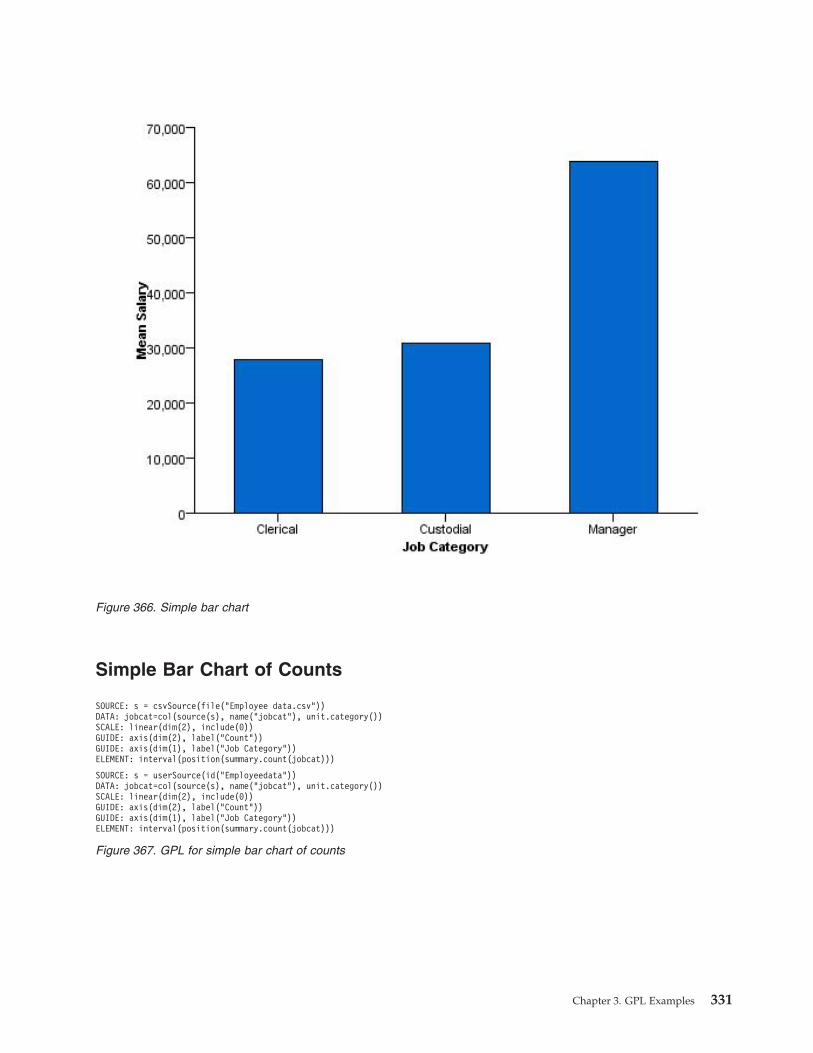
Simple Bar Chart of Counts

Figure 366. Simple bar chart

SOURCE: s = csvSource(file("Employee data.csv"))DATA: jobcat=col(source(s), name("jobcat"), unit.category())SCALE: linear(dim(2), include(0))GUIDE: axis(dim(2), label("Count"))GUIDE: axis(dim(1), label("Job Category"))ELEMENT: interval(position(summary.count(jobcat)))

SOURCE: s = userSource(id("Employeedata"))DATA: jobcat=col(source(s), name("jobcat"), unit.category())SCALE: linear(dim(2), include(0))GUIDE: axis(dim(2), label("Count"))GUIDE: axis(dim(1), label("Job Category"))ELEMENT: interval(position(summary.count(jobcat)))

Figure 367. GPL for simple bar chart of counts

Chapter 3. GPL Examples 331

Simple Horizontal Bar Chart

Figure 368. Simple bar chart of counts

SOURCE: s = csvSource(file("Employee data.csv"))DATA: jobcat=col(source(s), name("jobcat"), unit.category())DATA: salary=col(source(s), name("salary"))SCALE: linear(dim(2), min(0.0))GUIDE: axis(dim(2), label("Mean Salary"))GUIDE: axis(dim(1), label("Job Category"))COORD: transpose()ELEMENT: interval(position(summary.mean(jobcat*salary)))

SOURCE: s = userSource(id("Employeedata"))DATA: jobcat=col(source(s), name("jobcat"), unit.category())DATA: salary=col(source(s), name("salary"))SCALE: linear(dim(2), min(0.0))GUIDE: axis(dim(2), label("Mean Salary"))GUIDE: axis(dim(1), label("Job Category"))COORD: transpose()ELEMENT: interval(position(summary.mean(jobcat*salary)))

Figure 369. GPL for simple horizontal bar chart


Simple Bar Chart With Error Bars

Figure 370. Simple horizontal bar chart

SOURCE: s = csvSource(file("Employee data.csv"))DATA: jobcat=col(source(s), name("jobcat"), unit.category())DATA: salary=col(source(s), name("salary"))SCALE: linear(dim(2), include(0))GUIDE: axis(dim(2), label("Mean Salary"))GUIDE: axis(dim(1), label("Job Category"))ELEMENT: interval(position(summary.mean(jobcat*salary)))ELEMENT: interval(position(region.confi.mean(jobcat*salary)),

shape(shape.ibeam), size(size.".4in"), color(color.black))

SOURCE: s = userSource(id("Employeedata"))DATA: jobcat=col(source(s), name("jobcat"), unit.category())DATA: salary=col(source(s), name("salary"))SCALE: linear(dim(2), include(0))GUIDE: axis(dim(2), label("Mean Salary"))GUIDE: axis(dim(1), label("Job Category"))ELEMENT: interval(position(summary.mean(jobcat*salary)))ELEMENT: interval(position(region.confi.mean(jobcat*salary)),

shape(shape.ibeam), size(size.".4in"), color(color.black))

Figure 371. GPL for simple bar chart with error bars


Simple Bar Chart with Bar for All Categories

Note: Using "All" as the string is arbitrary. Any string would work (e.g., "Total" or "All Categories").Because it is blended with the jobcat categorical variable, the string acts like a new categorical value. Thisvalue is the same for all cases in the dataset. Therefore, the bar associated with that string shows theresult for all cases in the dataset.

Figure 372. Simple bar chart with error bars

SOURCE: s = csvSource(file("Employee data.csv"))DATA: jobcat=col(source(s), name("jobcat"), unit.category())DATA: salary=col(source(s), name("salary"))SCALE: linear(dim(2), include(0))GUIDE: axis(dim(2), label("Mean Salary"))GUIDE: axis(dim(1), label("Job Category"))ELEMENT: interval(position(summary.mean((jobcat+"All")*salary)))

SOURCE: s = userSource(id("Employeedata"))DATA: jobcat=col(source(s), name("jobcat"), unit.category())DATA: salary=col(source(s), name("salary"))SCALE: linear(dim(2), include(0))GUIDE: axis(dim(2), label("Mean Salary"))GUIDE: axis(dim(1), label("Job Category"))ELEMENT: interval(position(summary.mean((jobcat+"All")*salary)))

Figure 373. GPL for simple bar chart with bar for all categories


Stacked Bar Chart

Figure 374. Simple bar chart with a bar for all categories

SOURCE: s = csvSource(file("Employee data.csv"))DATA: jobcat=col(source(s), name("jobcat"), unit.category())DATA: gender=col(source(s), name("gender"), unit.category())SCALE: linear(dim(2), include(0))GUIDE: axis(dim(2), label("Count"))GUIDE: axis(dim(1), label("Job Category"))ELEMENT: interval.stack(position(summary.count(jobcat)),

color(gender))

SOURCE: s = userSource(id("Employeedata"))DATA: jobcat=col(source(s), name("jobcat"), unit.category())DATA: gender=col(source(s), name("gender"), unit.category())SCALE: linear(dim(2), include(0))GUIDE: axis(dim(2), label("Count"))GUIDE: axis(dim(1), label("Job Category"))ELEMENT: interval.stack(position(summary.count(jobcat)),

color(gender))

Figure 375. GPL for stacked bar chart


Clustered Bar Chart

Figure 376. Stacked bar chart

SOURCE: s = csvSource(file("Employee data.csv"))DATA: jobcat=col(source(s), name("jobcat"), unit.category())DATA: gender=col(source(s), name("gender"), unit.category())DATA: salary=col(source(s), name("salary"))COORD: rect(dim(1,2), cluster(3))SCALE: linear(dim(2), include(0))GUIDE: axis(dim(2), label("Mean Salary"))GUIDE: axis(dim(3), label("Gender"))ELEMENT: interval(position(summary.mean(jobcat*salary*gender)), color(jobcat))


Figure 377. GPL for clustered bar chart


Following is another option for creating a graph that appears clustered. It uses the dodge collisionmodifier. (See “dodge Collision Modifier” on page 54.) Note that the difference between this and theprevious example is that empty space is not allocated for missing categories (in this case, the combinationof "Female" and "Custodial").


SOURCE: s = csvSource(file("Employee data.csv"))DATA: jobcat=col(source(s), name("jobcat"), unit.category())DATA: gender=col(source(s), name("gender"), unit.category())DATA: salary=col(source(s), name("salary"))SCALE: linear(dim(2), include(0))GUIDE: axis(dim(2), label("Mean Salary"))GUIDE: axis(dim(1), label("Gender"))ELEMENT: interval.dodge(position(summary.mean(gender*salary)),

size(size."25%"), color(jobcat))

SOURCE: s = userSource(id("Employeedata"))DATA: jobcat=col(source(s), name("jobcat"), unit.category())DATA: gender=col(source(s), name("gender"), unit.category())DATA: salary=col(source(s), name("salary"))SCALE: linear(dim(2), include(0))GUIDE: axis(dim(2), label("Mean Salary"))GUIDE: axis(dim(1), label("Gender"))ELEMENT: interval.dodge(position(summary.mean(gender*salary)),

size(size."25%"), color(jobcat))

Figure 379. GPL for dodged bar chart


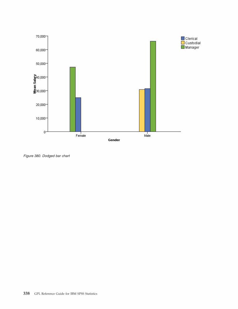
Figure 380. Dodged bar chart


Clustered and Stacked Bar Chart

SOURCE: s = csvSource(file("Employee data.csv"))DATA: jobcat = col(source(s), name("jobcat"), unit.category())DATA: gender = col(source(s), name("gender"), unit.category())DATA: minority = col(source(s), name("minority"), unit.category())DATA: salary = col(source(s), name("salary"))COORD: rect(dim(1, 2), cluster(3, 0))SCALE: linear(dim(2), include(0))GUIDE: axis(dim(2), label("Sum Salary"))GUIDE: axis(dim(3), label("Job Category"))GUIDE: legend(aesthetic(aesthetic.color.interior), label("Gender"))GUIDE: legend(aesthetic(aesthetic.texture.pattern.interior),

label("Minority Classification"))ELEMENT: interval.stack(position(summary.sum(gender*salary*jobcat)),

color.exterior(color.black),color.interior(gender), texture.pattern.interior(minority))

SOURCE: s = userSource(id("Employeedata"))DATA: jobcat = col(source(s), name("jobcat"), unit.category())DATA: gender = col(source(s), name("gender"), unit.category())DATA: minority = col(source(s), name("minority"), unit.category())DATA: salary = col(source(s), name("salary"))COORD: rect(dim(1, 2), cluster(3, 0))SCALE: linear(dim(2), include(0))GUIDE: axis(dim(2), label("Sum Salary"))GUIDE: axis(dim(3), label("Job Category"))GUIDE: legend(aesthetic(aesthetic.color.interior), label("Gender"))GUIDE: legend(aesthetic(aesthetic.texture.pattern.interior),

label("Minority Classification"))ELEMENT: interval.stack(position(summary.sum(gender*salary*jobcat)),

color.exterior(color.black),color.interior(gender), texture.pattern.interior(minority))

Figure 381. GPL for clustered and stacked bar chart

Figure 382. Clustered and stacked bar chart


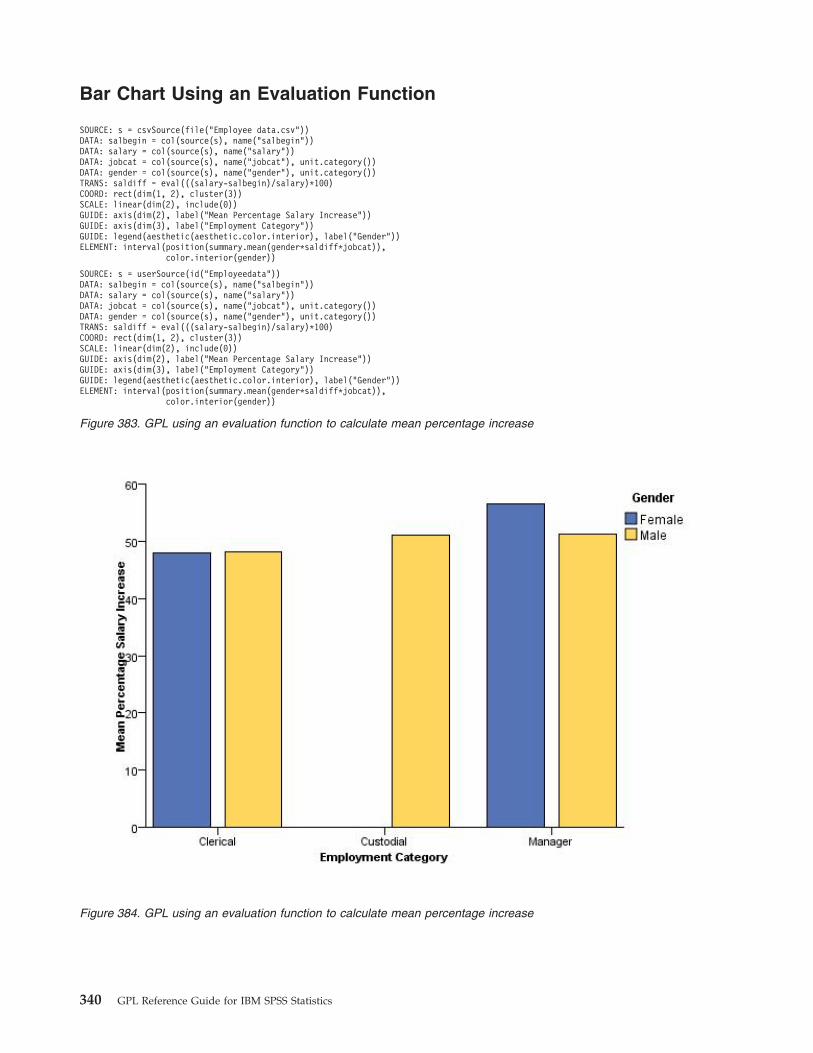
Bar Chart Using an Evaluation Function

SOURCE: s = csvSource(file("Employee data.csv"))DATA: salbegin = col(source(s), name("salbegin"))DATA: salary = col(source(s), name("salary"))DATA: jobcat = col(source(s), name("jobcat"), unit.category())DATA: gender = col(source(s), name("gender"), unit.category())TRANS: saldiff = eval(((salary-salbegin)/salary)*100)COORD: rect(dim(1, 2), cluster(3))SCALE: linear(dim(2), include(0))GUIDE: axis(dim(2), label("Mean Percentage Salary Increase"))GUIDE: axis(dim(3), label("Employment Category"))GUIDE: legend(aesthetic(aesthetic.color.interior), label("Gender"))ELEMENT: interval(position(summary.mean(gender*saldiff*jobcat)),

color.interior(gender))

SOURCE: s = userSource(id("Employeedata"))DATA: salbegin = col(source(s), name("salbegin"))DATA: salary = col(source(s), name("salary"))DATA: jobcat = col(source(s), name("jobcat"), unit.category())DATA: gender = col(source(s), name("gender"), unit.category())TRANS: saldiff = eval(((salary-salbegin)/salary)*100)COORD: rect(dim(1, 2), cluster(3))SCALE: linear(dim(2), include(0))GUIDE: axis(dim(2), label("Mean Percentage Salary Increase"))GUIDE: axis(dim(3), label("Employment Category"))GUIDE: legend(aesthetic(aesthetic.color.interior), label("Gender"))ELEMENT: interval(position(summary.mean(gender*saldiff*jobcat)),

color.interior(gender))

Figure 383. GPL using an evaluation function to calculate mean percentage increase

Figure 384. GPL using an evaluation function to calculate mean percentage increase


Bar Chart with Mapped AestheticsThis example demonstrates how you can map a specific categorical value in the graph to a specificaesthetic value. In this case, "Female" bars are colored green in the resulting graph.

SOURCE: s = csvSource(file("Employee data.csv"))DATA: salary = col(source(s), name("salary"))DATA: jobcat = col(source(s), name("jobcat"), unit.category())TRANS: greaterThan = eval(salary < 40000)SCALE: linear(dim(2), include(0))GUIDE: axis(dim(1), label("Employment Category"))GUIDE: axis(dim(2), label("% < 40000 Salary"))ELEMENT: interval(position(summary.percentTrue(jobcat*greaterThan)))

SOURCE: s = userSource(id("Employeedata"))DATA: salary = col(source(s), name("salary"))DATA: jobcat = col(source(s), name("jobcat"), unit.category())TRANS: greaterThan = eval(salary < 40000)SCALE: linear(dim(2), include(0))GUIDE: axis(dim(1), label("Employment Category"))GUIDE: axis(dim(2), label("% < 40000 Salary"))ELEMENT: interval(position(summary.percentTrue(jobcat*greaterThan)))

Figure 385. GPL using an evaluation function to calculate percent less than a value

Figure 386. GPL using an evaluation function to calculate percent less than a value


Faceted (Paneled) Bar ChartAlthough the following examples create bar charts, faceting is common to all graphs.

SOURCE: s = csvSource(file("Employee data.csv"))DATA: salary = col(source(s), name("salary"))DATA: jobcat = col(source(s), name("jobcat"), unit.category())DATA: gender = col(source(s), name("gender"), unit.category())COORD: rect(dim(1, 2), cluster(3))SCALE: cat(aesthetic(aesthetic.color), map(("Female", color.green)))GUIDE: axis(dim(2), label("Mean Salary"))GUIDE: axis(dim(3), label("Job Category"))ELEMENT: interval(position(summary.mean(gender*salary*jobcat)),

color(gender))

SOURCE: s = userSource(id("Employeedata"))DATA: salary = col(source(s), name("salary"))DATA: jobcat = col(source(s), name("jobcat"), unit.category())DATA: gender = col(source(s), name("gender"), unit.category())COORD: rect(dim(1, 2), cluster(3))SCALE: cat(aesthetic(aesthetic.color), map(("Female", color.green)))GUIDE: axis(dim(2), label("Mean Salary"))GUIDE: axis(dim(3), label("Job Category"))ELEMENT: interval(position(summary.mean(gender*salary*jobcat)),

color(gender))SCALE: cat(aesthetic(aesthetic.color), map(("f", color.green)))GUIDE: axis(dim(2), label("Mean Salary"))GUIDE: axis(dim(3), label("Job Category"))ELEMENT: interval(position(summary.mean(gender*salary*jobcat)),

color(gender))

Figure 387. GPL for bar chart with mapped aesthetics

Figure 388. Bar chart with mapped aesthetics


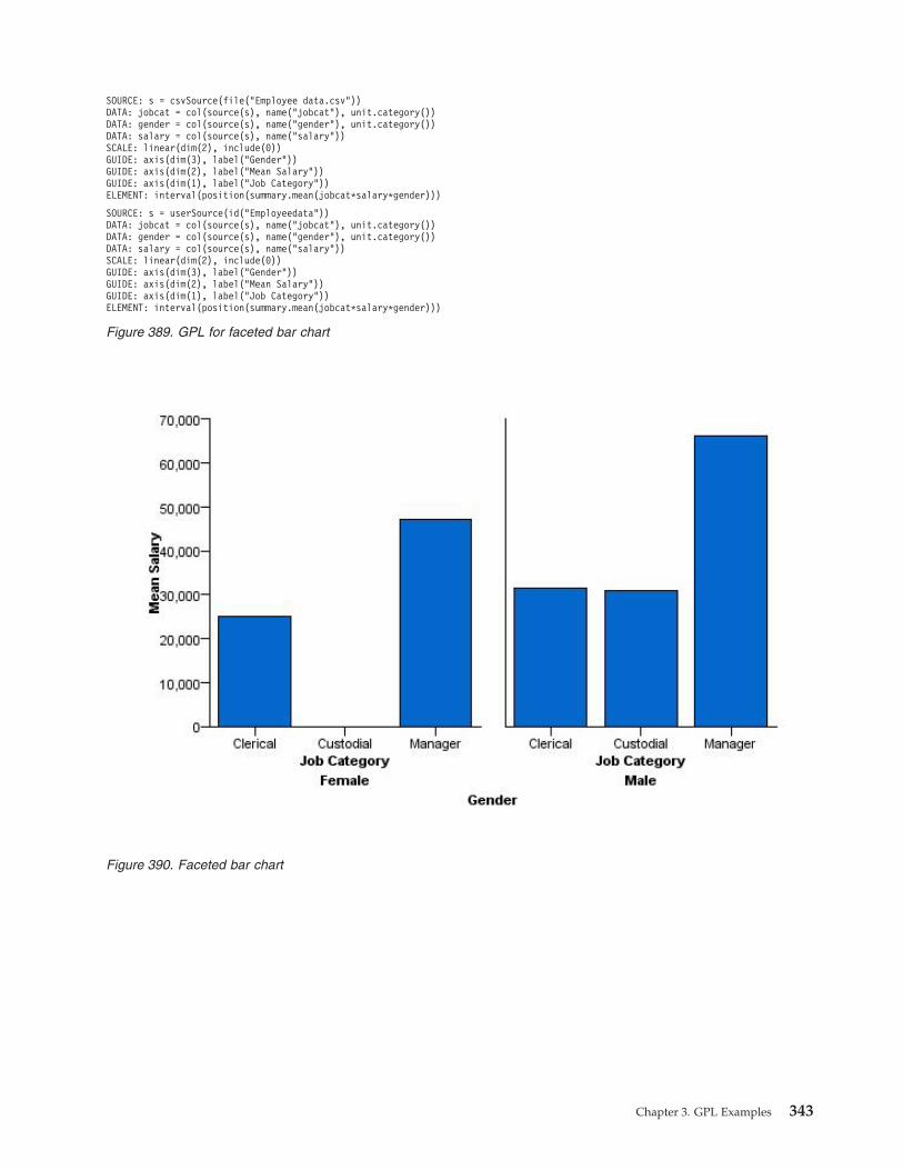
SOURCE: s = csvSource(file("Employee data.csv"))DATA: jobcat = col(source(s), name("jobcat"), unit.category())DATA: gender = col(source(s), name("gender"), unit.category())DATA: salary = col(source(s), name("salary"))SCALE: linear(dim(2), include(0))GUIDE: axis(dim(3), label("Gender"))GUIDE: axis(dim(2), label("Mean Salary"))GUIDE: axis(dim(1), label("Job Category"))ELEMENT: interval(position(summary.mean(jobcat*salary*gender)))

SOURCE: s = userSource(id("Employeedata"))DATA: jobcat = col(source(s), name("jobcat"), unit.category())DATA: gender = col(source(s), name("gender"), unit.category())DATA: salary = col(source(s), name("salary"))SCALE: linear(dim(2), include(0))GUIDE: axis(dim(3), label("Gender"))GUIDE: axis(dim(2), label("Mean Salary"))GUIDE: axis(dim(1), label("Job Category"))ELEMENT: interval(position(summary.mean(jobcat*salary*gender)))

Figure 389. GPL for faceted bar chart



SOURCE: s = csvSource(file("Employee data.csv"))DATA: jobcat = col(source(s), name("jobcat"), unit.category())DATA: gender = col(source(s), name("gender"), unit.category())DATA: salary = col(source(s), name("salary"))SCALE: linear(dim(2), include(0.0))GUIDE: axis(dim(2), label("Mean Salary"))GUIDE: axis(dim(1.1), label("Job Category"))GUIDE: axis(dim(1), label("Gender"))ELEMENT: interval(position(summary.mean(jobcat/gender*salary)))

SOURCE: s = userSource(id("Employeedata"))DATA: jobcat = col(source(s), name("jobcat"), unit.category())DATA: gender = col(source(s), name("gender"), unit.category())DATA: salary = col(source(s), name("salary"))SCALE: linear(dim(2), include(0.0))GUIDE: axis(dim(2), label("Mean Salary"))GUIDE: axis(dim(1.1), label("Job Category"))GUIDE: axis(dim(1), label("Gender"))ELEMENT: interval(position(summary.mean(jobcat/gender*salary)))

Figure 391. GPL for faceted bar chart with nested categories

Figure 392. Faceted bar chart with nested categories


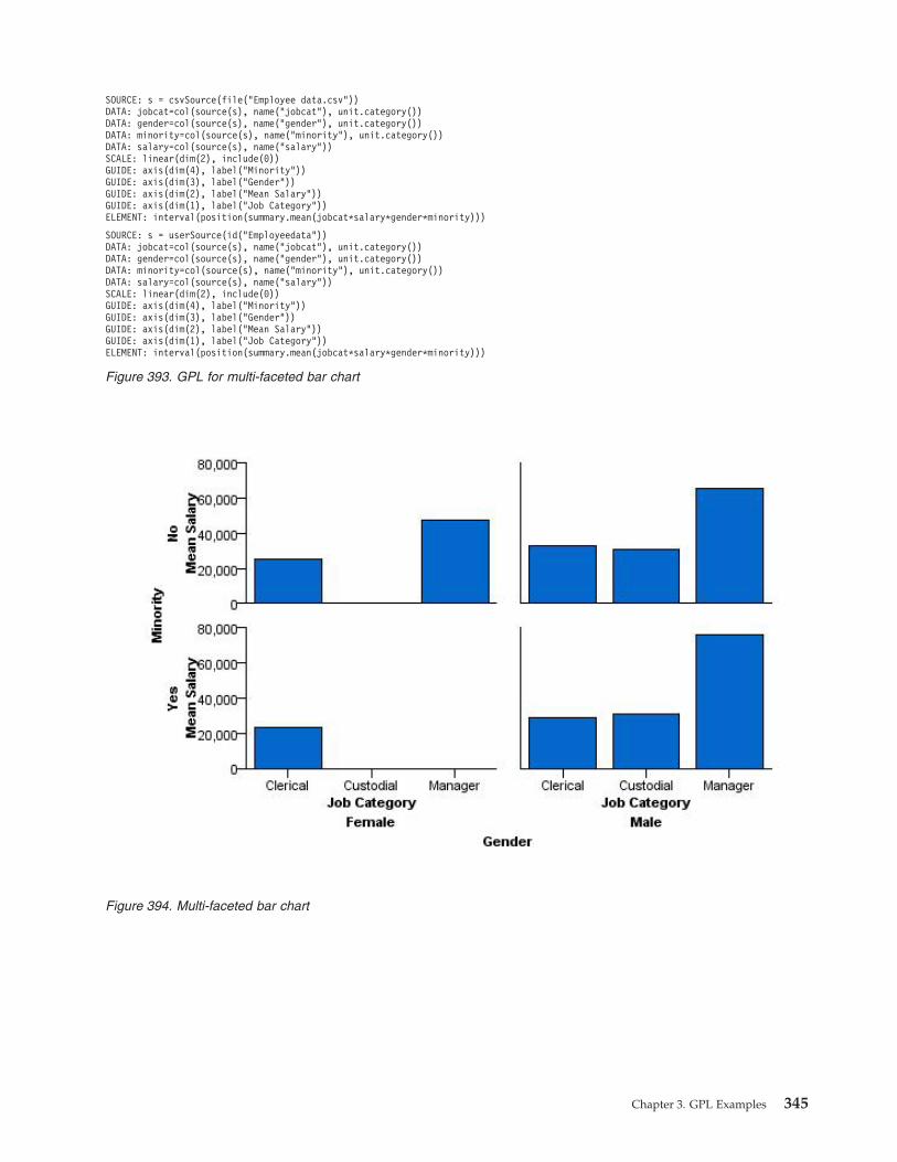
SOURCE: s = csvSource(file("Employee data.csv"))DATA: jobcat=col(source(s), name("jobcat"), unit.category())DATA: gender=col(source(s), name("gender"), unit.category())DATA: minority=col(source(s), name("minority"), unit.category())DATA: salary=col(source(s), name("salary"))SCALE: linear(dim(2), include(0))GUIDE: axis(dim(4), label("Minority"))GUIDE: axis(dim(3), label("Gender"))GUIDE: axis(dim(2), label("Mean Salary"))GUIDE: axis(dim(1), label("Job Category"))ELEMENT: interval(position(summary.mean(jobcat*salary*gender*minority)))

SOURCE: s = userSource(id("Employeedata"))DATA: jobcat=col(source(s), name("jobcat"), unit.category())DATA: gender=col(source(s), name("gender"), unit.category())DATA: minority=col(source(s), name("minority"), unit.category())DATA: salary=col(source(s), name("salary"))SCALE: linear(dim(2), include(0))GUIDE: axis(dim(4), label("Minority"))GUIDE: axis(dim(3), label("Gender"))GUIDE: axis(dim(2), label("Mean Salary"))GUIDE: axis(dim(1), label("Job Category"))ELEMENT: interval(position(summary.mean(jobcat*salary*gender*minority)))

Figure 393. GPL for multi-faceted bar chart

Figure 394. Multi-faceted bar chart


3-D Bar Chart

SOURCE: s = csvSource(file("Employee data.csv"))DATA: jobcat=col(source(s), name("jobcat"), unit.category())DATA: gender=col(source(s), name("gender"), unit.category())DATA: salary=col(source(s), name("salary"))COORD: rect(dim(1,2,3))SCALE: linear(dim(3), include(0))GUIDE: axis(dim(3), label("Mean Salary"))GUIDE: axis(dim(2), label("Gender"))GUIDE: axis(dim(1), label("Job Category"))ELEMENT: interval(position(summary.mean(jobcat*gender*salary)))

SOURCE: s = userSource(id("Employeedata"))DATA: jobcat=col(source(s), name("jobcat"), unit.category())DATA: gender=col(source(s), name("gender"), unit.category())DATA: salary=col(source(s), name("salary"))COORD: rect(dim(1,2,3))SCALE: linear(dim(3), include(0))GUIDE: axis(dim(3), label("Mean Salary"))GUIDE: axis(dim(2), label("Gender"))GUIDE: axis(dim(1), label("Job Category"))ELEMENT: interval(position(summary.mean(jobcat*gender*salary)))

Figure 395. GPL for 3-D bar chart

Figure 396. 3-D bar chart


Error Bar Chart

Histogram ExamplesThis section provides examples of different types of histograms.

SOURCE: s = csvSource(file("Employee data.csv"))DATA: salary = col(source(s), name("salary"))DATA: jobcat=col(source(s), name("jobcat"), unit.category())GUIDE: axis(dim(2), label("Mean +- 1 SD Current Salary"))GUIDE: axis(dim(1), label("Job Category"))ELEMENT: interval(position(region.confi.mean(jobcat*salary)),

shape(shape.ibeam), size(size.".4in"))ELEMENT: point(position(summary.mean(jobcat*salary)),

shape(shape.circle), color(color.red), size(size."6px"))

SOURCE: s = userSource(id("Employeedata"))DATA: salary = col(source(s), name("salary"))DATA: jobcat=col(source(s), name("jobcat"), unit.category())GUIDE: axis(dim(2), label("Mean +- 1 SD Current Salary"))GUIDE: axis(dim(1), label("Job Category"))ELEMENT: interval(position(region.confi.mean(jobcat*salary)),

shape(shape.ibeam), size(size.".4in"))ELEMENT: point(position(summary.mean(jobcat*salary)),

shape(shape.circle), color(color.red), size(size."6px"))

Figure 397. GPL for error bar chart

Figure 398. Error bar chart


Histogram

SOURCE: s = csvSource(file("Employee data.csv"))DATA: salary=col(source(s), name("salary"))GUIDE: axis(dim(2), label("Count"))GUIDE: axis(dim(1), label("Salary"))ELEMENT: interval(position(summary.count(bin.rect(salary))))

SOURCE: s = userSource(id("Employeedata"))DATA: salary=col(source(s), name("salary"))GUIDE: axis(dim(2), label("Count"))GUIDE: axis(dim(1), label("Salary"))ELEMENT: interval(position(summary.count(bin.rect(salary))))

Figure 399. GPL for histogram

Figure 400. Histogram


Histogram with Distribution Curve

SOURCE: s = csvSource(file("Employee data.csv"))DATA: salary=col(source(s), name("salary"))GUIDE: axis(dim(2), label("Count"))GUIDE: axis(dim(1), label("Salary"))ELEMENT: interval(position(summary.count(bin.rect(salary))))ELEMENT: line(position(density.normal(salary)))

SOURCE: s = userSource(id("Employeedata"))DATA: salary=col(source(s), name("salary"))GUIDE: axis(dim(2), label("Count"))GUIDE: axis(dim(1), label("Salary"))ELEMENT: interval(position(summary.count(bin.rect(salary))))ELEMENT: line(position(density.normal(salary)))

Figure 401. GPL for histogram with normal curve

Figure 402. Histogram with normal curve


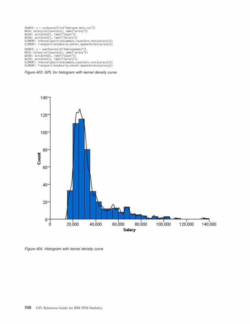
SOURCE: s = csvSource(file("Employee data.csv"))DATA: salary=col(source(s), name("salary"))GUIDE: axis(dim(2), label("Count"))GUIDE: axis(dim(1), label("Salary"))ELEMENT: interval(position(summary.count(bin.rect(salary))))ELEMENT: line(position(density.kernel.epanechnikov(salary)))

SOURCE: s = userSource(id("Employeedata"))DATA: salary=col(source(s), name("salary"))GUIDE: axis(dim(2), label("Count"))GUIDE: axis(dim(1), label("Salary"))ELEMENT: interval(position(summary.count(bin.rect(salary))))ELEMENT: line(position(density.kernel.epanechnikov(salary)))

Figure 403. GPL for histogram with kernel density curve

Figure 404. Histogram with kernel density curve


Percentage Histogram

SOURCE: s = csvSource(file("Employee data.csv"))DATA: salary = col(source(s), name("salary"))GUIDE: axis(dim(2), label("Percent"))GUIDE: axis(dim(1), label("Salary"))ELEMENT: interval(position(summary.percent.count(bin.rect(salary))))

SOURCE: s = userSource(id("Employeedata"))DATA: salary = col(source(s), name("salary"))GUIDE: axis(dim(2), label("Percent"))GUIDE: axis(dim(1), label("Salary"))ELEMENT: interval(position(summary.percent.count(bin.rect(salary))))

Figure 405. GPL for percentage histogram

Figure 406. Percentage histogram


Frequency Polygon

SOURCE: s = csvSource(file("Employee data.csv"))DATA: salary=col(source(s), name("salary"))GUIDE: axis(dim(2), label("Count"))GUIDE: axis(dim(1), label("Salary"))ELEMENT: area(position(summary.count(bin.rect(salary))))

SOURCE: s = userSource(id("Employeedata"))DATA: salary=col(source(s), name("salary"))GUIDE: axis(dim(2), label("Count"))GUIDE: axis(dim(1), label("Salary"))ELEMENT: area(position(summary.count(bin.rect(salary))))

Figure 407. GPL for frequency polygon

Figure 408. Frequency polygon


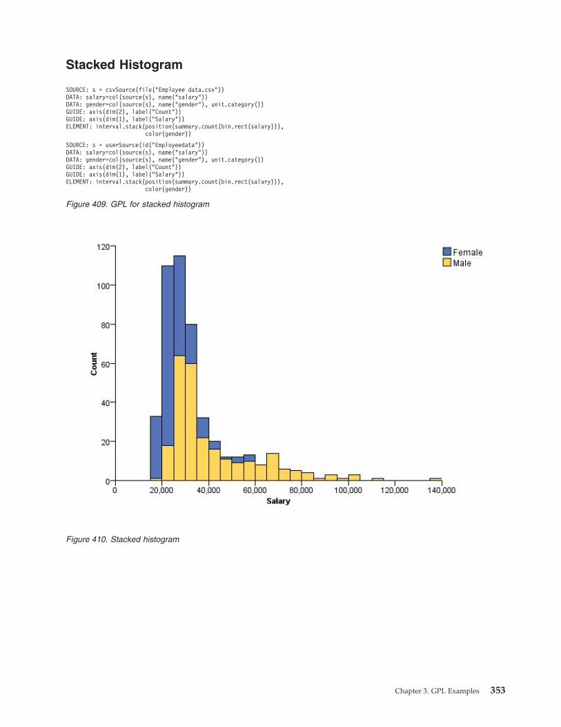
Stacked Histogram

SOURCE: s = csvSource(file("Employee data.csv"))DATA: salary=col(source(s), name("salary"))DATA: gender=col(source(s), name("gender"), unit.category())GUIDE: axis(dim(2), label("Count"))GUIDE: axis(dim(1), label("Salary"))ELEMENT: interval.stack(position(summary.count(bin.rect(salary))),

color(gender))

SOURCE: s = userSource(id("Employeedata"))DATA: salary=col(source(s), name("salary"))DATA: gender=col(source(s), name("gender"), unit.category())GUIDE: axis(dim(2), label("Count"))GUIDE: axis(dim(1), label("Salary"))ELEMENT: interval.stack(position(summary.count(bin.rect(salary))),

color(gender))

Figure 409. GPL for stacked histogram

Figure 410. Stacked histogram


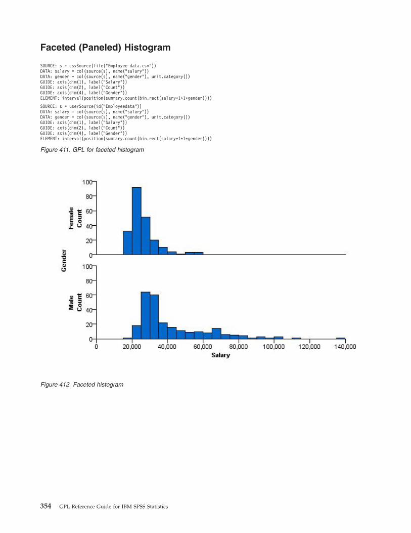
Faceted (Paneled) Histogram

SOURCE: s = csvSource(file("Employee data.csv"))DATA: salary = col(source(s), name("salary"))DATA: gender = col(source(s), name("gender"), unit.category())GUIDE: axis(dim(1), label("Salary"))GUIDE: axis(dim(2), label("Count"))GUIDE: axis(dim(4), label("Gender"))ELEMENT: interval(position(summary.count(bin.rect(salary*1*1*gender))))

SOURCE: s = userSource(id("Employeedata"))DATA: salary = col(source(s), name("salary"))DATA: gender = col(source(s), name("gender"), unit.category())GUIDE: axis(dim(1), label("Salary"))GUIDE: axis(dim(2), label("Count"))GUIDE: axis(dim(4), label("Gender"))ELEMENT: interval(position(summary.count(bin.rect(salary*1*1*gender))))

Figure 411. GPL for faceted histogram

Figure 412. Faceted histogram


Population Pyramid

SOURCE: s = csvSource(file("Employee data.csv"))DATA: gender = col(source(s), name("gender"), unit.category())DATA: salary = col(source(s), name("salary"))COORD: transpose(mirror())GUIDE: axis(dim(1), label("Current Salary"))GUIDE: axis(dim(1), label(""), opposite())GUIDE: axis(dim(2), label("Frequency"))GUIDE: axis(dim(3), label("Gender"), opposite(), gap(0px))GUIDE: legend(aesthetic(aesthetic.color.interior), null())ELEMENT: interval(position(summary.count(bin.rect(salary*1*gender))), color(gender))

SOURCE: s = userSource(id("Employeedata"))DATA: gender = col(source(s), name("gender"), unit.category())DATA: salary = col(source(s), name("salary"))COORD: transpose(mirror())GUIDE: axis(dim(1), label("Current Salary"))GUIDE: axis(dim(1), label(""), opposite())GUIDE: axis(dim(2), label("Frequency"))GUIDE: axis(dim(3), label("Gender"), opposite(), gap(0px))GUIDE: legend(aesthetic(aesthetic.color.interior), null())ELEMENT: interval(position(summary.count(bin.rect(salary*1*gender))), color(gender))

Figure 413. GPL for population pyramid

Figure 414. Population pyramid


Cumulative Histogram

SOURCE: s = csvSource(file("Employee data.csv"))DATA: salary=col(source(s), name("salary"))GUIDE: axis(dim(2), label("Cumulative Percent"))GUIDE: axis(dim(1), label("Salary"))ELEMENT: interval(position(summary.percent.count.cumulative(bin.rect(salary))))

SOURCE: s = userSource(id("Employeedata"))DATA: salary=col(source(s), name("salary"))GUIDE: axis(dim(2), label("Cumulative Percent"))GUIDE: axis(dim(1), label("Salary"))ELEMENT: interval(position(summary.percent.count.cumulative(bin.rect(salary))))

Figure 415. GPL for cumulative histogram

Figure 416. Cumulative histogram


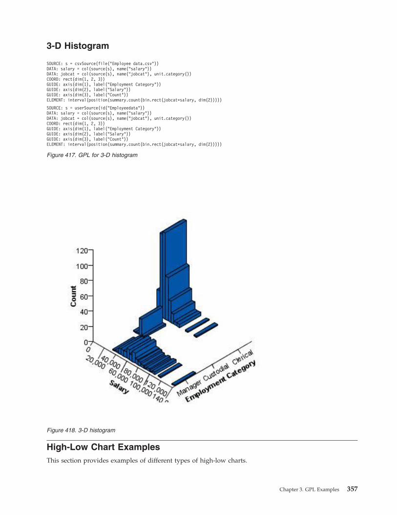
3-D Histogram

High-Low Chart ExamplesThis section provides examples of different types of high-low charts.

SOURCE: s = csvSource(file("Employee data.csv"))DATA: salary = col(source(s), name("salary"))DATA: jobcat = col(source(s), name("jobcat"), unit.category())COORD: rect(dim(1, 2, 3))GUIDE: axis(dim(1), label("Employment Category"))GUIDE: axis(dim(2), label("Salary"))GUIDE: axis(dim(3), label("Count"))ELEMENT: interval(position(summary.count(bin.rect(jobcat*salary, dim(2)))))

SOURCE: s = userSource(id("Employeedata"))DATA: salary = col(source(s), name("salary"))DATA: jobcat = col(source(s), name("jobcat"), unit.category())COORD: rect(dim(1, 2, 3))GUIDE: axis(dim(1), label("Employment Category"))GUIDE: axis(dim(2), label("Salary"))GUIDE: axis(dim(3), label("Count"))ELEMENT: interval(position(summary.count(bin.rect(jobcat*salary, dim(2)))))

Figure 417. GPL for 3-D histogram

Figure 418. 3-D histogram


Simple Range Bar for One Variable

SOURCE: s = csvSource(file("Employee data.csv"))DATA: jobcat=col(source(s), name("jobcat"), unit.category())DATA: salary=col(source(s), name("salary"))SCALE: linear(dim(2), min(0.0))GUIDE: axis(dim(2), label("Min Current Salary - Max Current Salary"))GUIDE: axis(dim(1), label("Job Category"))ELEMENT: interval(position(region.spread.range(jobcat*salary)))

SOURCE: s = userSource(id("Employeedata"))DATA: jobcat=col(source(s), name("jobcat"), unit.category())DATA: salary=col(source(s), name("salary"))SCALE: linear(dim(2), min(0.0))GUIDE: axis(dim(2), label("Min Current Salary - Max Current Salary"))GUIDE: axis(dim(1), label("Job Category"))ELEMENT: interval(position(region.spread.range(jobcat*salary)))

Figure 419. GPL for simple range bar for one variable

Figure 420. Simple range bar for one variable


Simple Range Bar for Two Variables

SOURCE: s = csvSource(file("Employee data.csv"))DATA: jobcat=col(source(s), name("jobcat"), unit.category())DATA: salbegin=col(source(s), name("salbegin"))DATA: salary=col(source(s), name("salary"))SCALE: linear(dim(2), min(0.0))GUIDE: axis(dim(2), label("Min Beginning Salary - Max Current Salary"))GUIDE: axis(dim(1), label("Job Category"))ELEMENT: interval(position(region.spread.range(jobcat*(salbegin+salary))))

SOURCE: s = userSource(id("Employeedata"))DATA: jobcat=col(source(s), name("jobcat"), unit.category())DATA: salbegin=col(source(s), name("salbegin"))DATA: salary=col(source(s), name("salary"))SCALE: linear(dim(2), min(0.0))GUIDE: axis(dim(2), label("Min Beginning Salary - Max Current Salary"))GUIDE: axis(dim(1), label("Job Category"))ELEMENT: interval(position(region.spread.range(jobcat*(salbegin+salary))))

Figure 421. GPL for simple range bar for two variables

Figure 422. Simple range bar for two variables


High-Low-Close Chart

SOURCE: s = csvSource(file("stocks.csv"))DATA: Date = col(source(s), name("Date"), unit.time(), format("MM/dd/yy"))DATA: Close = col(source(s), name("Close"))DATA: High = col(source(s), name("High"))DATA: Low = col(source(s), name("Low"))GUIDE: axis(dim(1), label("Date"))GUIDE: axis(dim(2), label("Close"))SCALE: time(dim(1), dataMaximum())ELEMENT: interval(position(region.spread.range(Date*(Low+High))))ELEMENT: point(position(Date*Close), color.exterior(color.red), size(size."2px"))

SOURCE: s = userSource(id("stocks"))DATA: Date = col(source(s), name("Date"), unit.time(), format("MM/dd/yy"))DATA: Close = col(source(s), name("Close"))DATA: High = col(source(s), name("High"))DATA: Low = col(source(s), name("Low"))GUIDE: axis(dim(1), label("Date"))GUIDE: axis(dim(2), label("Close"))SCALE: time(dim(1), dataMaximum())ELEMENT: interval(position(region.spread.range(Date*(Low+High))))ELEMENT: point(position(Date*Close), color.exterior(color.red), size(size."2px"))

Figure 423. GPL for high-low-close chart

Figure 424. High-low-close chart


Scatter/Dot ExamplesThis section provides examples of different types of scatterplots and dot plots.

Simple 1-D Scatterplot

SOURCE: s = csvSource(file("Employee data.csv"))DATA: salary = col(source(s), name("salary"))COORD: rect(dim(1))GUIDE: axis(dim(1), label("Salary"))ELEMENT: point(position(salary))

SOURCE: s = userSource(id("Employeedata"))DATA: salary = col(source(s), name("salary"))COORD: rect(dim(1))GUIDE: axis(dim(1), label("Salary"))ELEMENT: point(position(salary))

Figure 425. GPL for simple 1-D scatterplot



Simple 2-D Scatterplot

SOURCE: s = csvSource(file("Employee data.csv"))DATA: salbegin=col(source(s), name("salbegin"))DATA: salary=col(source(s), name("salary"))GUIDE: axis(dim(2), label("Current Salary"))GUIDE: axis(dim(1), label("Beginning Salary"))ELEMENT: point(position(salbegin*salary))


Figure 427. GPL for simple 2-D scatterplot



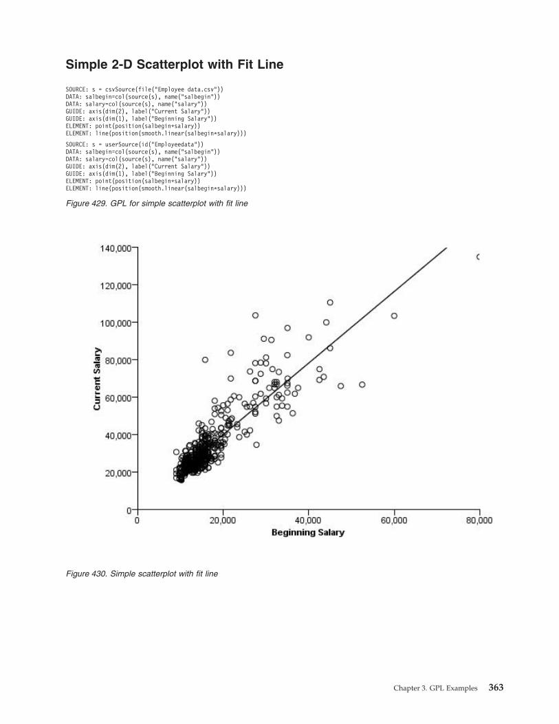
Simple 2-D Scatterplot with Fit Line

SOURCE: s = csvSource(file("Employee data.csv"))DATA: salbegin=col(source(s), name("salbegin"))DATA: salary=col(source(s), name("salary"))GUIDE: axis(dim(2), label("Current Salary"))GUIDE: axis(dim(1), label("Beginning Salary"))ELEMENT: point(position(salbegin*salary))ELEMENT: line(position(smooth.linear(salbegin*salary)))

SOURCE: s = userSource(id("Employeedata"))DATA: salbegin=col(source(s), name("salbegin"))DATA: salary=col(source(s), name("salary"))GUIDE: axis(dim(2), label("Current Salary"))GUIDE: axis(dim(1), label("Beginning Salary"))ELEMENT: point(position(salbegin*salary))ELEMENT: line(position(smooth.linear(salbegin*salary)))

Figure 429. GPL for simple scatterplot with fit line

Figure 430. Simple scatterplot with fit line


Grouped Scatterplot

SOURCE: s = csvSource(file("Employee data.csv"))DATA: salbegin=col(source(s), name("salbegin"))DATA: salary=col(source(s), name("salary"))DATA: gender=col(source(s), name("gender"), unit.category())GUIDE: axis(dim(2), label("Current Salary"))GUIDE: axis(dim(1), label("Beginning Salary"))ELEMENT: point(position(salbegin*salary), color(gender))

SOURCE: s = userSource(id("Employeedata"))DATA: salbegin=col(source(s), name("salbegin"))DATA: salary=col(source(s), name("salary"))DATA: gender=col(source(s), name("gender"), unit.category())GUIDE: axis(dim(2), label("Current Salary"))GUIDE: axis(dim(1), label("Beginning Salary"))ELEMENT: point(position(salbegin*salary), color(gender))

Figure 431. GPL for grouped scatterplot

Figure 432. Grouped scatterplot


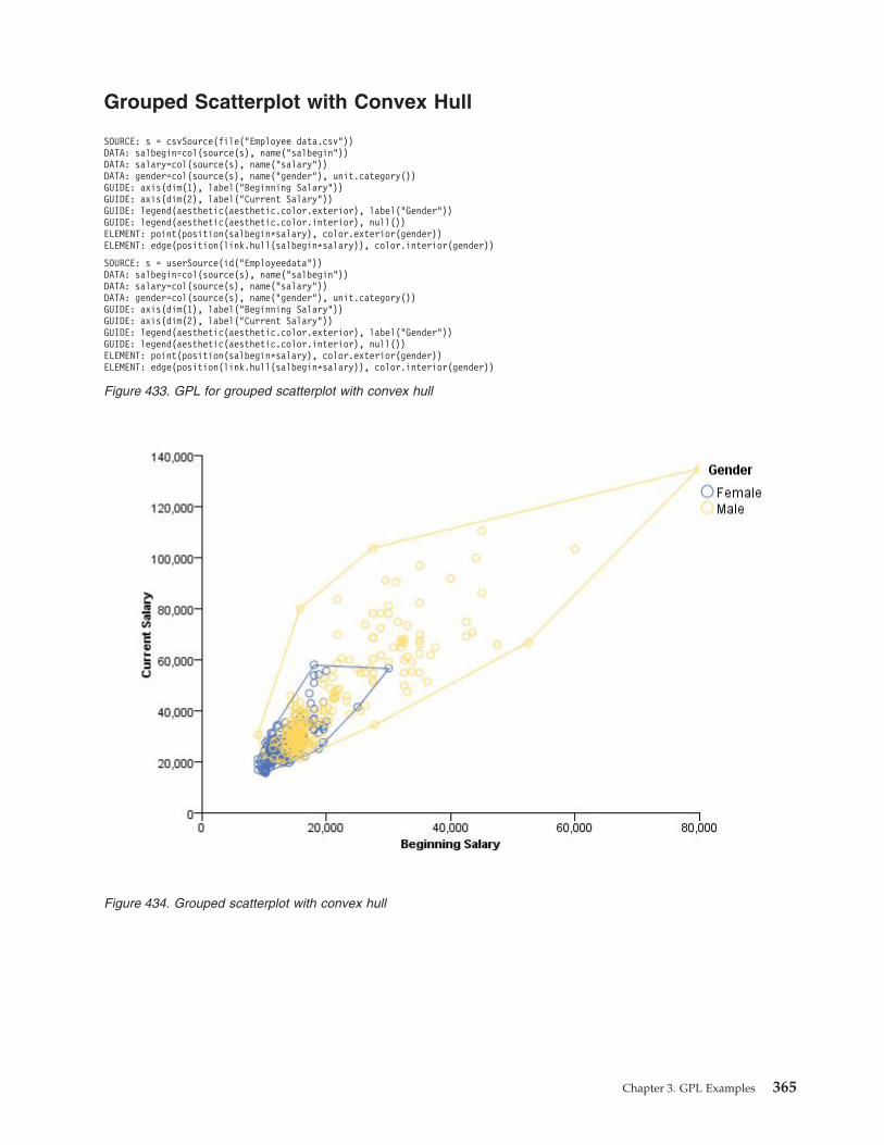
Grouped Scatterplot with Convex Hull

SOURCE: s = csvSource(file("Employee data.csv"))DATA: salbegin=col(source(s), name("salbegin"))DATA: salary=col(source(s), name("salary"))DATA: gender=col(source(s), name("gender"), unit.category())GUIDE: axis(dim(1), label("Beginning Salary"))GUIDE: axis(dim(2), label("Current Salary"))GUIDE: legend(aesthetic(aesthetic.color.exterior), label("Gender"))GUIDE: legend(aesthetic(aesthetic.color.interior), null())ELEMENT: point(position(salbegin*salary), color.exterior(gender))ELEMENT: edge(position(link.hull(salbegin*salary)), color.interior(gender))

SOURCE: s = userSource(id("Employeedata"))DATA: salbegin=col(source(s), name("salbegin"))DATA: salary=col(source(s), name("salary"))DATA: gender=col(source(s), name("gender"), unit.category())GUIDE: axis(dim(1), label("Beginning Salary"))GUIDE: axis(dim(2), label("Current Salary"))GUIDE: legend(aesthetic(aesthetic.color.exterior), label("Gender"))GUIDE: legend(aesthetic(aesthetic.color.interior), null())ELEMENT: point(position(salbegin*salary), color.exterior(gender))ELEMENT: edge(position(link.hull(salbegin*salary)), color.interior(gender))

Figure 433. GPL for grouped scatterplot with convex hull

Figure 434. Grouped scatterplot with convex hull


Scatterplot Matrix (SPLOM)

SOURCE: s = csvSource(file("customer_subset.csv"))DATA: age=col(source(s), name("age"))DATA: income=col(source(s), name("income"))DATA: creddebt=col(source(s), name("creddebt"))GUIDE: axis(dim(1.1), ticks(null()))GUIDE: axis(dim(2.1), ticks(null()))GUIDE: axis(dim(1), gap(0px))GUIDE: axis(dim(2), gap(0px))ELEMENT: point(position((age/"Age"+income/"Income"+creddebt/"CC Debt")*

(age/"Age"+income/"Income"+creddebt/"CC Debt")))

SOURCE: s = userSource(id("customer_subset"))DATA: age=col(source(s), name("age"))DATA: income=col(source(s), name("income"))DATA: creddebt=col(source(s), name("creddebt"))GUIDE: axis(dim(1.1), ticks(null()))GUIDE: axis(dim(2.1), ticks(null()))GUIDE: axis(dim(1), gap(0px))GUIDE: axis(dim(2), gap(0px))ELEMENT: point(position((age/"Age"+income/"Income"+creddebt/"CC Debt")*

(age/"Age"+income/"Income"+creddebt/"CC Debt")))

Figure 435. GPL for scatterplot matrix

Figure 436. Scatterplot Matrix


Bubble Plot

SOURCE: s = csvSource(file("Employee data.csv"))DATA: salbegin=col(source(s), name("salbegin"))DATA: salary=col(source(s), name("salary"))DATA: prevexp=col(source(s), name("prevexp"))SCALE: linear(aesthetic(aesthetic.size),

aestheticMinimum(size."5px"), aestheticMaximum(size."35px"))GUIDE: axis(dim(2), label("Current Salary"))GUIDE: axis(dim(1), label("Beginning Salary"))GUIDE: legend(aesthetic(aesthetic.size), label("Previous Experience (months)"))ELEMENT: point(position(salbegin*salary), size(prevexp))

SOURCE: s = userSource(id("Employeedata"))DATA: salbegin=col(source(s), name("salbegin"))DATA: salary=col(source(s), name("salary"))DATA: prevexp=col(source(s), name("prevexp"))SCALE: linear(aesthetic(aesthetic.size),

aestheticMinimum(size."5px"), aestheticMaximum(size."35px"))GUIDE: axis(dim(2), label("Current Salary"))GUIDE: axis(dim(1), label("Beginning Salary"))GUIDE: legend(aesthetic(aesthetic.size), label("Previous Experience (months)"))ELEMENT: point(position(salbegin*salary), size(prevexp))

Figure 437. GPL for bubble plot

Figure 438. Bubble plot


Binned Scatterplot

SOURCE: s = csvSource(file("Employee data.csv"))DATA: salbegin=col(source(s), name("salbegin"))DATA: salary=col(source(s), name("salary"))GUIDE: axis(dim(2), label("Current Salary"))GUIDE: axis(dim(1), label("Beginning Salary"))GUIDE: legend(aesthetic(aesthetic.color), label("Count"))ELEMENT: point(position(bin.rect(salbegin*salary, dim(1,2))),

color(summary.count()))

SOURCE: s = userSource(id("Employeedata"))DATA: salbegin=col(source(s), name("salbegin"))DATA: salary=col(source(s), name("salary"))GUIDE: axis(dim(2), label("Current Salary"))GUIDE: axis(dim(1), label("Beginning Salary"))GUIDE: legend(aesthetic(aesthetic.color), label("Count"))ELEMENT: point(position(bin.rect(salbegin*salary, dim(1,2))),


Figure 439. GPL for binned scatterplot

Figure 440. Binned scatterplot


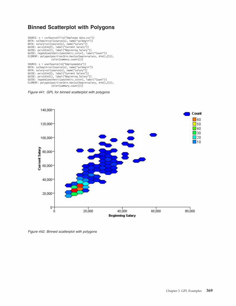
Binned Scatterplot with Polygons

SOURCE: s = csvSource(file("Employee data.csv"))DATA: salbegin=col(source(s), name("salbegin"))DATA: salary=col(source(s), name("salary"))GUIDE: axis(dim(2), label("Current Salary"))GUIDE: axis(dim(1), label("Beginning Salary"))GUIDE: legend(aesthetic(aesthetic.color), label("Count"))ELEMENT: polygon(position(bin.hex(salbegin*salary, dim(1,2))),


SOURCE: s = userSource(id("Employeedata"))DATA: salbegin=col(source(s), name("salbegin"))DATA: salary=col(source(s), name("salary"))GUIDE: axis(dim(2), label("Current Salary"))GUIDE: axis(dim(1), label("Beginning Salary"))GUIDE: legend(aesthetic(aesthetic.color), label("Count"))ELEMENT: polygon(position(bin.hex(salbegin*salary, dim(1,2))),


Figure 441. GPL for binned scatterplot with polygons

Figure 442. Binned scatterplot with polygons


Scatterplot with Border Histograms

SOURCE: s = csvSource(file("Employee data.csv"))DATA: salary = col(source(s), name("salary"))DATA: salbegin = col(source(s), name("salbegin"))GRAPH: begin(origin(5%, 10%), scale(85%, 85%))GUIDE: axis(dim(1), label("Beginning Salary"))GUIDE: axis(dim(2), label("Current Salary"))ELEMENT: point(position(salbegin*salary))GRAPH: end()GRAPH: begin(origin(5%, 0%), scale(85%, 10%))GUIDE: axis(dim(1), ticks(null()))GUIDE: axis(dim(2), null())ELEMENT: interval(position(summary.count(bin.rect(salbegin))))GRAPH: end()GRAPH: begin(origin(90%, 10%), scale(10%, 85%))COORD: rect(dim(1, 2), transpose())GUIDE: axis(dim(1), ticks(null()))GUIDE: axis(dim(2), null())ELEMENT: interval(position(summary.count(bin.rect(salary))))GRAPH: end()

SOURCE: s = userSource(id("Employeedata"))DATA: salary = col(source(s), name("salary"))DATA: salbegin = col(source(s), name("salbegin"))GRAPH: begin(origin(5%, 10%), scale(85%, 85%))GUIDE: axis(dim(1), label("Beginning Salary"))GUIDE: axis(dim(2), label("Current Salary"))ELEMENT: point(position(salbegin*salary))GRAPH: end()GRAPH: begin(origin(5%, 0%), scale(85%, 10%))GUIDE: axis(dim(1), ticks(null()))GUIDE: axis(dim(2), null())ELEMENT: interval(position(summary.count(bin.rect(salbegin))))GRAPH: end()GRAPH: begin(origin(90%, 10%), scale(10%, 85%))COORD: rect(dim(1, 2), transpose())GUIDE: axis(dim(1), ticks(null()))GUIDE: axis(dim(2), null())ELEMENT: interval(position(summary.count(bin.rect(salary))))GRAPH: end()

Figure 443. GPL for scatterplot with border histograms


Scatterplot with Border Boxplots

SOURCE: s = csvSource(file("Employee data.csv"))DATA: salary = col(source(s), name("salary"))DATA: salbegin = col(source(s), name("salbegin"))GRAPH: begin(origin(5%, 10%), scale(85%, 85%))GUIDE: axis(dim(1), label("Beginning Salary"))GUIDE: axis(dim(2), label("Current Salary"))ELEMENT: point(position(salbegin*salary))GRAPH: end()GRAPH: begin(origin(5%, 0%), scale(85%, 10%))COORD: rect(dim(1))GUIDE: axis(dim(1), ticks(null()))ELEMENT: schema(position(bin.quantile.letter(salbegin)), size(size."80%"))GRAPH: end()GRAPH: begin(origin(90%, 10%), scale(10%, 85%))COORD: transpose(rect(dim(1)))GUIDE: axis(dim(1), ticks(null()))ELEMENT: schema(position(bin.quantile.letter(salary)), size(size."80%"))GRAPH: end()

SOURCE: s = userSource(id("Employeedata"))DATA: salary = col(source(s), name("salary"))DATA: salbegin = col(source(s), name("salbegin"))GRAPH: begin(origin(5%, 10%), scale(85%, 85%))GUIDE: axis(dim(1), label("Beginning Salary"))GUIDE: axis(dim(2), label("Current Salary"))ELEMENT: point(position(salbegin*salary))GRAPH: end()GRAPH: begin(origin(5%, 0%), scale(85%, 10%))COORD: rect(dim(1))GUIDE: axis(dim(1), ticks(null()))ELEMENT: schema(position(bin.quantile.letter(salbegin)), size(size."80%"))GRAPH: end()GRAPH: begin(origin(90%, 10%), scale(10%, 85%))COORD: transpose(rect(dim(1)))GUIDE: axis(dim(1), ticks(null()))ELEMENT: schema(position(bin.quantile.letter(salary)), size(size."80%"))GRAPH: end()

Figure 444. GPL for scatterplot with border boxplots


Dot Plot

Figure 445. Scatterplot with border boxplots

SOURCE: s = csvSource(file("Employee data.csv"))DATA: salary = col(source(s), name("salary"))COORD: rect(dim(1))GUIDE: axis(dim(1), label("Salary"))ELEMENT: point.dodge.asymmetric(position(bin.dot(salary)))

SOURCE: s = userSource(id("Employeedata"))DATA: salary = col(source(s), name("salary"))COORD: rect(dim(1))GUIDE: axis(dim(1), label("Salary"))ELEMENT: point.dodge.asymmetric(position(bin.dot(salary)))

Figure 446. GPL for dot plot


Figure 447. Dot plot

SOURCE: s = csvSource(file("Employee data.csv"))DATA: gender = col(source(s), name("gender"), unit.category())DATA: salary = col(source(s), name("salary"))GUIDE: axis(dim(1), label("Salary"))COORD: rect(dim(1))ELEMENT: point.dodge.asymmetric(position(bin.dot(salary)),

color(gender), shape(shape.square))

SOURCE: s = userSource(id("Employeedata"))DATA: gender = col(source(s), name("gender"), unit.category())DATA: salary = col(source(s), name("salary"))GUIDE: axis(dim(1), label("Salary"))COORD: rect(dim(1))ELEMENT: point.dodge.asymmetric(position(bin.dot(salary)),

color(gender), shape(shape.square))

Figure 448. GPL for grouped dot plot


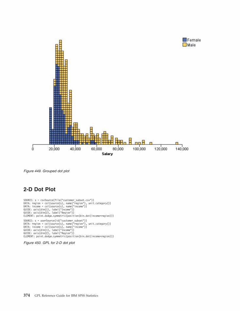
2-D Dot Plot

Figure 449. Grouped dot plot

SOURCE: s = csvSource(file("customer_subset.csv"))DATA: region = col(source(s), name("region"), unit.category())DATA: income = col(source(s), name("income"))GUIDE: axis(dim(1), label("Income"))GUIDE: axis(dim(2), label("Region"))ELEMENT: point.dodge.symmetric(position(bin.dot(income*region)))

SOURCE: s = userSource(id("customer_subset"))DATA: region = col(source(s), name("region"), unit.category())DATA: income = col(source(s), name("income"))GUIDE: axis(dim(1), label("Income"))GUIDE: axis(dim(2), label("Region"))ELEMENT: point.dodge.symmetric(position(bin.dot(income*region)))

Figure 450. GPL for 2-D dot plot


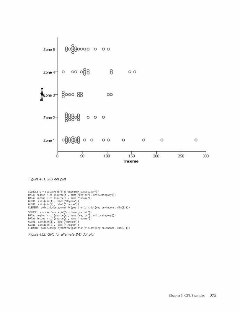
Figure 451. 2-D dot plot

SOURCE: s = csvSource(file("customer_subset.csv"))DATA: region = col(source(s), name("region"), unit.category())DATA: income = col(source(s), name("income"))GUIDE: axis(dim(1), label("Region"))GUIDE: axis(dim(2), label("Income"))ELEMENT: point.dodge.symmetric(position(bin.dot(region*income, dim(2))))

SOURCE: s = userSource(id("customer_subset"))DATA: region = col(source(s), name("region"), unit.category())DATA: income = col(source(s), name("income"))GUIDE: axis(dim(1), label("Region"))GUIDE: axis(dim(2), label("Income"))ELEMENT: point.dodge.symmetric(position(bin.dot(region*income, dim(2))))

Figure 452. GPL for alternate 2-D dot plot


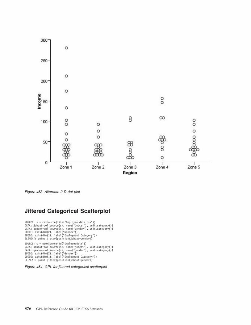
Jittered Categorical Scatterplot

Figure 453. Alternate 2-D dot plot

SOURCE: s = csvSource(file("Employee data.csv"))DATA: jobcat=col(source(s), name("jobcat"), unit.category())DATA: gender=col(source(s), name("gender"), unit.category())GUIDE: axis(dim(2), label("Gender"))GUIDE: axis(dim(1), label("Employment Category"))ELEMENT: point.jitter(position(jobcat*gender))

SOURCE: s = userSource(id("Employeedata"))DATA: jobcat=col(source(s), name("jobcat"), unit.category())DATA: gender=col(source(s), name("gender"), unit.category())GUIDE: axis(dim(2), label("Gender"))GUIDE: axis(dim(1), label("Employment Category"))ELEMENT: point.jitter(position(jobcat*gender))

Figure 454. GPL for jittered categorical scatterplot


Line Chart ExamplesThis section provides examples of different types of line charts.

Simple Line Chart

Figure 455. Jittered categorical scatterplot

SOURCE: s = csvSource(file("Employee data.csv"))DATA: salbegin=col(source(s), name("salbegin"))DATA: salary=col(source(s), name("salary"))GUIDE: axis(dim(2), label("Current Salary"))GUIDE: axis(dim(1), label("Beginning Salary"))ELEMENT: line(position(salbegin*salary))

SOURCE: s = userSource(id("Employeedata"))DATA: salbegin=col(source(s), name("salbegin"))DATA: salary=col(source(s), name("salary"))GUIDE: axis(dim(2), label("Current Salary"))GUIDE: axis(dim(1), label("Beginning Salary"))ELEMENT: line(position(salbegin*salary))

Figure 456. GPL for simple line chart


Simple Line Chart with Points

Figure 457. Simple line chart

SOURCE: s = csvSource(file("Employee data.csv"))DATA: salbegin=col(source(s), name("salbegin"))DATA: salary=col(source(s), name("salary"))GUIDE: axis(dim(2), label("Current Salary"))GUIDE: axis(dim(1), label("Beginning Salary"))ELEMENT: line(position(salbegin*salary))ELEMENT: point(position(salbegin*salary))

SOURCE: s = userSource(id("Employeedata"))DATA: salbegin=col(source(s), name("salbegin"))DATA: salary=col(source(s), name("salary"))GUIDE: axis(dim(2), label("Current Salary"))GUIDE: axis(dim(1), label("Beginning Salary"))ELEMENT: line(position(salbegin*salary))ELEMENT: point(position(salbegin*salary))

Figure 458. GPL for simple line chart with points


Line Chart of Date Data

Figure 459. Simple line chart with points

SOURCE: s = csvSource(file("stocks.csv"))DATA: Date = col(source(s), name("Date"), unit.time(), format("MM/dd/yy"))DATA: Close = col(source(s), name("Close"))GUIDE: axis(dim(1), label("Date"))GUIDE: axis(dim(2), label("Close"))SCALE: time(dim(1), dataMaximum())ELEMENT: line(position(Date*Close))

SOURCE: s = userSource(id("stocks"))DATA: Date = col(source(s), name("Date"), unit.time(), format("MM/dd/yy"))DATA: Close = col(source(s), name("Close"))GUIDE: axis(dim(1), label("Date"))GUIDE: axis(dim(2), label("Close"))SCALE: time(dim(1), dataMaximum())ELEMENT: line(position(Date*Close))

Figure 460. GPL for line chart of date data


Line Chart With Step Interpolation

Figure 461. Line chart of date data

SOURCE: s = csvSource(file("Employee data.csv"))DATA: salbegin=col(source(s), name("salbegin"))DATA: salary=col(source(s), name("salary"))GUIDE: axis(dim(2), label("Current Salary"))GUIDE: axis(dim(1), label("Beginning Salary"))ELEMENT: line(position(smooth.step.center(salbegin*salary)))

SOURCE: s = userSource(id("Employeedata"))DATA: salbegin=col(source(s), name("salbegin"))DATA: salary=col(source(s), name("salary"))GUIDE: axis(dim(2), label("Current Salary"))GUIDE: axis(dim(1), label("Beginning Salary"))ELEMENT: line(position(smooth.step.center(salbegin*salary)))

Figure 462. GPL for line chart with step interpolation


Fit Line

Figure 463. Line chart with step interpolation

SOURCE: s = csvSource(file("Employee data.csv"))DATA: salbegin=col(source(s), name("salbegin"))DATA: salary=col(source(s), name("salary"))GUIDE: axis(dim(2), label("Current Salary"))GUIDE: axis(dim(1), label("Beginning Salary"))ELEMENT: point(position(salbegin*salary))ELEMENT: line(position(smooth.linear(salbegin*salary)))

SOURCE: s = userSource(id("Employeedata"))DATA: salbegin=col(source(s), name("salbegin"))DATA: salary=col(source(s), name("salary"))GUIDE: axis(dim(2), label("Current Salary"))GUIDE: axis(dim(1), label("Beginning Salary"))ELEMENT: point(position(salbegin*salary))ELEMENT: line(position(smooth.linear(salbegin*salary)))

Figure 464. GPL for linear fit line overlaid on scatterplot


Line Chart from Equation

Figure 465. Linear fit line overlaid on scatterplot

DATA: x = iter(0,10,0.01)TRANS: y = eval(sin(x)*cos(x)*(x-5))ELEMENT: line(position(x*y))

Figure 466. GPL for line chart from equation


Figure 467. Line chart from equation

DATA: x = iter(0,6.28,0.01)TRANS: y = eval(cos(6*x))COORD: polar()SCALE: linear(dim(1), min(0.0), max(6.28))GUIDE: axis(dim(2), null())ELEMENT: line(position(x*y))

Figure 468. GPL for line chart from equation in polar coordinates


Line Chart with Separate Scales

Figure 469. Line chart from equation in polar coordinates

SOURCE: s = csvSource(file("stocks.csv"))DATA: date = col(source(s), name("Date"), unit.time(), format("MM/dd/yy"))DATA: close = col(source(s), name("Close"))DATA: volume = col(source(s), name("Volume"))SCALE: time(dim(1), dataMaximum())ELEMENT: line(position(date*(close/"Close"+volume/"Volume")))

SOURCE: s = userSource(id("stocks"))DATA: date = col(source(s), name("Date"), unit.time(), format("MM/dd/yy"))DATA: close = col(source(s), name("Close"))DATA: volume = col(source(s), name("Volume"))SCALE: time(dim(1), dataMaximum())ELEMENT: line(position(date*(close/"Close"+volume/"Volume")))

Figure 470. GPL for line chart with separate scales


Pie Chart ExamplesThis section provides examples of different types of pie charts.

Pie Chart

Figure 471. Line chart with separate scales

SOURCE: s = csvSource(file("Employee data.csv"))DATA: jobcat=col(source(s), name("jobcat"), unit.category())COORD: polar.theta()SCALE: linear(dim(1), dataMinimum(), dataMaximum())GUIDE: axis(dim(1), null())ELEMENT: interval.stack(position(summary.count(1)), color(jobcat))

SOURCE: s = userSource(id("Employeedata"))DATA: jobcat=col(source(s), name("jobcat"), unit.category())COORD: polar.theta()SCALE: linear(dim(1), dataMinimum(), dataMaximum())GUIDE: axis(dim(1), null())ELEMENT: interval.stack(position(summary.count(1)), color(jobcat))

Figure 472. GPL for pie chart


Figure 473. Pie chart

SOURCE: s = csvSource(file("Employee data.csv"))DATA: jobcat=col(source(s), name("jobcat"), unit.category())COORD: polar.theta()SCALE: linear(dim(1), dataMinimum(), dataMaximum())GUIDE: axis(dim(1), null())GUIDE: legend(aesthetic(aesthetic.color), null())ELEMENT: interval.stack(position(summary.count(1)), color(jobcat),

label(jobcat))

SOURCE: s = userSource(id("Employeedata"))DATA: jobcat=col(source(s), name("jobcat"), unit.category())COORD: polar.theta()SCALE: linear(dim(1), dataMinimum(), dataMaximum())GUIDE: axis(dim(1), null())GUIDE: legend(aesthetic(aesthetic.color), null())ELEMENT: interval.stack(position(summary.count(1)), color(jobcat),

label(jobcat))

Figure 474. GPL for pie chart with labels


Paneled Pie Chart

Figure 475. Pie chart with labels

SOURCE: s = csvSource(file("Employee data.csv"))DATA: jobcat = col(source(s), name("jobcat"), unit.category())DATA: gender = col(source(s), name("gender"), unit.category())COORD: polar.theta()SCALE: linear(dim(1), dataMinimum(), dataMaximum())GUIDE: axis(dim(1), null())GUIDE: axis(dim(2), label("Gender"))ELEMENT: interval.stack(position(summary.percent.count(1*gender))),

color(jobcat))

SOURCE: s = userSource(id("Employeedata"))DATA: jobcat = col(source(s), name("jobcat"), unit.category())DATA: gender = col(source(s), name("gender"), unit.category())COORD: polar.theta()SCALE: linear(dim(1), dataMinimum(), dataMaximum())GUIDE: axis(dim(1), null())GUIDE: axis(dim(2), label("Gender"))ELEMENT: interval.stack(position(summary.percent.count(1*gender))),

color(jobcat))

Figure 476. GPL for paneled pie chart


Stacked Pie Chart

Figure 477. Paneled pie chart

SOURCE: s = csvSource(file("Employee data.csv"))DATA: jobcat = col(source(s), name("jobcat"), unit.category())DATA: gender = col(source(s), name("gender"), unit.category())COORD: polar(transpose())GUIDE: axis(dim(1), null())GUIDE: axis(dim(2), null())GUIDE: legend(aesthetic(aesthetic.texture.pattern.interior), label("Employment Category"))GUIDE: legend(aesthetic(aesthetic.color.interior), label("Gender"))ELEMENT: interval.stack(position(summary.percent.count(jobcat*1, base.coordinate(dim(1)))),

texture.pattern(jobcat), color(gender), size(size."100%"))

SOURCE: s = userSource(id("Employeedata"))DATA: jobcat = col(source(s), name("jobcat"), unit.category())DATA: gender = col(source(s), name("gender"), unit.category())COORD: polar(transpose())GUIDE: axis(dim(1), null())GUIDE: axis(dim(2), null())GUIDE: legend(aesthetic(aesthetic.texture.pattern.interior), label("Employment Category"))GUIDE: legend(aesthetic(aesthetic.color.interior), label("Gender"))ELEMENT: interval.stack(position(summary.percent.count(jobcat*1, base.coordinate(dim(1)))),

texture.pattern(jobcat), color(gender), size(size."100%"))

Figure 478. GPL for stacked pie chart


Boxplot ExamplesThis section provides examples of different types of box plots.

1-D Boxplot

Figure 479. Stacked pie chart

SOURCE: s = csvSource(file("Employee data.csv"))DATA: salary = col(source(s), name("salary"))COORD: rect(dim(1))GUIDE: axis(dim(1), label("Salary"))ELEMENT: schema(position(bin.quantile.letter(salary)), size(size."50%"))

SOURCE: s = userSource(id("Employeedata"))DATA: salary = col(source(s), name("salary"))COORD: rect(dim(1))GUIDE: axis(dim(1), label("Salary"))ELEMENT: schema(position(bin.quantile.letter(salary)), size(size."50%"))

Figure 480. GPL for 1-D box plot


Boxplot

Figure 481. 1-D boxplot

SOURCE: s = csvSource(file("Employee data.csv"))DATA: jobcat=col(source(s), name("jobcat"), unit.category())DATA: salary=col(source(s), name("salary"))GUIDE: axis(dim(2), label("Salary"))GUIDE: axis(dim(1), label("Job Category"))ELEMENT: schema(position(bin.quantile.letter(jobcat*salary)))

SOURCE: s = userSource(id("Employeedata"))DATA: jobcat=col(source(s), name("jobcat"), unit.category())DATA: salary=col(source(s), name("salary"))GUIDE: axis(dim(2), label("Salary"))GUIDE: axis(dim(1), label("Job Category"))ELEMENT: schema(position(bin.quantile.letter(jobcat*salary)))

Figure 482. GPL for boxplot


Figure 483. Boxplot

SOURCE: s = csvSource(file("Employee data.csv"))DATA: jobcat=col(source(s), name("jobcat"), unit.category())DATA: salary=col(source(s), name("salary"))DATA: id = col(source(s), name("id"), unit.category())GUIDE: axis(dim(2), label("Salary"))GUIDE: axis(dim(1), label("Job Category"))ELEMENT: schema(position(bin.quantile.letter(jobcat*salary)), label(id))

SOURCE: s = userSource(id("Employeedata"))DATA: jobcat=col(source(s), name("jobcat"), unit.category())DATA: salary=col(source(s), name("salary"))DATA: id = col(source(s), name("id"), unit.category())GUIDE: axis(dim(2), label("Salary"))GUIDE: axis(dim(1), label("Job Category"))ELEMENT: schema(position(bin.quantile.letter(jobcat*salary)), label(id))

Figure 484. GPL for boxplot with labeled outliers


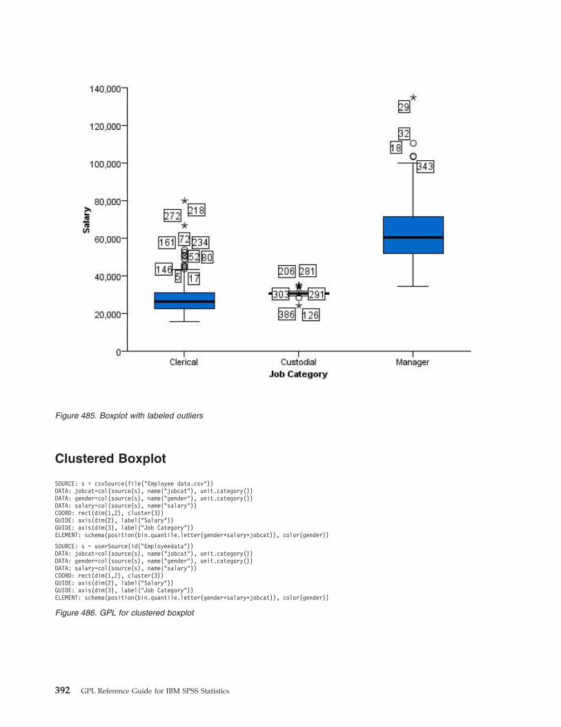
Clustered Boxplot

Figure 485. Boxplot with labeled outliers

SOURCE: s = csvSource(file("Employee data.csv"))DATA: jobcat=col(source(s), name("jobcat"), unit.category())DATA: gender=col(source(s), name("gender"), unit.category())DATA: salary=col(source(s), name("salary"))COORD: rect(dim(1,2), cluster(3))GUIDE: axis(dim(2), label("Salary"))GUIDE: axis(dim(3), label("Job Category"))ELEMENT: schema(position(bin.quantile.letter(gender*salary*jobcat)), color(gender))

SOURCE: s = userSource(id("Employeedata"))DATA: jobcat=col(source(s), name("jobcat"), unit.category())DATA: gender=col(source(s), name("gender"), unit.category())DATA: salary=col(source(s), name("salary"))COORD: rect(dim(1,2), cluster(3))GUIDE: axis(dim(2), label("Salary"))GUIDE: axis(dim(3), label("Job Category"))ELEMENT: schema(position(bin.quantile.letter(gender*salary*jobcat)), color(gender))

Figure 486. GPL for clustered boxplot


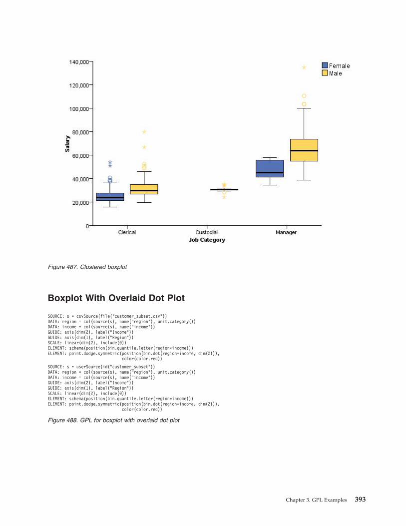
Boxplot With Overlaid Dot Plot

Figure 487. Clustered boxplot

SOURCE: s = csvSource(file("customer_subset.csv"))DATA: region = col(source(s), name("region"), unit.category())DATA: income = col(source(s), name("income"))GUIDE: axis(dim(2), label("Income"))GUIDE: axis(dim(1), label("Region"))SCALE: linear(dim(2), include(0))ELEMENT: schema(position(bin.quantile.letter(region*income)))ELEMENT: point.dodge.symmetric(position(bin.dot(region*income, dim(2))),

color(color.red))

SOURCE: s = userSource(id("customer_subset"))DATA: region = col(source(s), name("region"), unit.category())DATA: income = col(source(s), name("income"))GUIDE: axis(dim(2), label("Income"))GUIDE: axis(dim(1), label("Region"))SCALE: linear(dim(2), include(0))ELEMENT: schema(position(bin.quantile.letter(region*income)))ELEMENT: point.dodge.symmetric(position(bin.dot(region*income, dim(2))),

color(color.red))

Figure 488. GPL for boxplot with overlaid dot plot


Multi-Graph ExamplesThis section provides examples of multiple graphs in the same page display.

Figure 489. Boxplot with overlaid dot plot


Scatterplot with Border Histograms

SOURCE: s = csvSource(file("Employee data.csv"))DATA: salary = col(source(s), name("salary"))DATA: salbegin = col(source(s), name("salbegin"))GRAPH: begin(origin(5%, 10%), scale(85%, 85%))GUIDE: axis(dim(1), label("Beginning Salary"))GUIDE: axis(dim(2), label("Current Salary"))ELEMENT: point(position(salbegin*salary))GRAPH: end()GRAPH: begin(origin(5%, 0%), scale(85%, 10%))GUIDE: axis(dim(1), ticks(null()))GUIDE: axis(dim(2), null())ELEMENT: interval(position(summary.count(bin.rect(salbegin))))GRAPH: end()GRAPH: begin(origin(90%, 10%), scale(10%, 85%))COORD: rect(dim(1, 2), transpose())GUIDE: axis(dim(1), ticks(null()))GUIDE: axis(dim(2), null())ELEMENT: interval(position(summary.count(bin.rect(salary))))GRAPH: end()

SOURCE: s = userSource(id("Employeedata"))DATA: salary = col(source(s), name("salary"))DATA: salbegin = col(source(s), name("salbegin"))GRAPH: begin(origin(5%, 10%), scale(85%, 85%))GUIDE: axis(dim(1), label("Beginning Salary"))GUIDE: axis(dim(2), label("Current Salary"))ELEMENT: point(position(salbegin*salary))GRAPH: end()GRAPH: begin(origin(5%, 0%), scale(85%, 10%))GUIDE: axis(dim(1), ticks(null()))GUIDE: axis(dim(2), null())ELEMENT: interval(position(summary.count(bin.rect(salbegin))))GRAPH: end()GRAPH: begin(origin(90%, 10%), scale(10%, 85%))COORD: rect(dim(1, 2), transpose())GUIDE: axis(dim(1), ticks(null()))GUIDE: axis(dim(2), null())ELEMENT: interval(position(summary.count(bin.rect(salary))))GRAPH: end()

Figure 490. GPL for scatterplot with border histograms


Figure 491. Scatterplot with border histograms


Scatterplot with Border Boxplots

SOURCE: s = csvSource(file("Employee data.csv"))DATA: salary = col(source(s), name("salary"))DATA: salbegin = col(source(s), name("salbegin"))GRAPH: begin(origin(5%, 10%), scale(85%, 85%))GUIDE: axis(dim(1), label("Beginning Salary"))GUIDE: axis(dim(2), label("Current Salary"))ELEMENT: point(position(salbegin*salary))GRAPH: end()GRAPH: begin(origin(5%, 0%), scale(85%, 10%))COORD: rect(dim(1))GUIDE: axis(dim(1), ticks(null()))ELEMENT: schema(position(bin.quantile.letter(salbegin)), size(size."80%"))GRAPH: end()GRAPH: begin(origin(90%, 10%), scale(10%, 85%))COORD: transpose(rect(dim(1)))GUIDE: axis(dim(1), ticks(null()))ELEMENT: schema(position(bin.quantile.letter(salary)), size(size."80%"))GRAPH: end()

SOURCE: s = userSource(id("Employeedata"))DATA: salary = col(source(s), name("salary"))DATA: salbegin = col(source(s), name("salbegin"))GRAPH: begin(origin(5%, 10%), scale(85%, 85%))GUIDE: axis(dim(1), label("Beginning Salary"))GUIDE: axis(dim(2), label("Current Salary"))ELEMENT: point(position(salbegin*salary))GRAPH: end()GRAPH: begin(origin(5%, 0%), scale(85%, 10%))COORD: rect(dim(1))GUIDE: axis(dim(1), ticks(null()))ELEMENT: schema(position(bin.quantile.letter(salbegin)), size(size."80%"))GRAPH: end()GRAPH: begin(origin(90%, 10%), scale(10%, 85%))COORD: transpose(rect(dim(1)))GUIDE: axis(dim(1), ticks(null()))ELEMENT: schema(position(bin.quantile.letter(salary)), size(size."80%"))GRAPH: end()

Figure 492. GPL for scatterplot with border boxplots


Figure 493. Scatterplot with border boxplots


Stocks Line Chart with Volume Bar Chart

SOURCE: s = csvSource(file("stocks.csv"))DATA: date = col(source(s), name("Date"), unit.time(), format("MM/dd/yy"))DATA: close = col(source(s), name("Close"))DATA: volume = col(source(s), name("Volume"))GRAPH: begin(origin(10%, 0%), scale(90%, 60%))GUIDE: axis(dim(1), ticks(null()))GUIDE: axis(dim(2), label("Close"))ELEMENT: line(position(date*close)))GRAPH: end()GRAPH: begin(origin(10%, 70%), scale(90%, 25%))GUIDE: axis(dim(1), label("Date"))GUIDE: axis(dim(2), label("Volume"))ELEMENT: interval(position(date*volume))GRAPH: end()

SOURCE: s = userSource(id("stocks"))DATA: date = col(source(s), name("Date"), unit.time(), format("MM/dd/yy"))DATA: close = col(source(s), name("Close"))DATA: volume = col(source(s), name("Volume"))GRAPH: begin(origin(10%, 0%), scale(90%, 60%))GUIDE: axis(dim(1), ticks(null()))GUIDE: axis(dim(2), label("Close"))ELEMENT: line(position(date*close)))GRAPH: end()GRAPH: begin(origin(10%, 70%), scale(90%, 25%))GUIDE: axis(dim(1), label("Date"))GUIDE: axis(dim(2), label("Volume"))ELEMENT: interval(position(date*volume))GRAPH: end()

Figure 494. GPL for stocks and volume chart


Dual Axis Graph

Figure 495. Stocks and volume chart

SOURCE: s = csvSource(file("Employee data.csv"))DATA: jobcat = col(source(s), name("jobcat"), unit.category())DATA: salary = col(source(s), name("salary"))SCALE: y1 = linear(dim(2), include(0.0))SCALE: y2 = linear(dim(2), include(0.0))GUIDE: axis(dim(1), label("Employment Category"))GUIDE: axis(scale(y1), label("Mean Salary"))GUIDE: axis(scale(y2), label("Count"), opposite(), color(color.red))ELEMENT: interval(position(summary.mean(jobcat*salary)), scale(y1))ELEMENT: line(position(summary.count(jobcat)), color(color.red), scale(y2))

SOURCE: s = userSource(id("Employeedata"))DATA: jobcat = col(source(s), name("jobcat"), unit.category())DATA: salary = col(source(s), name("salary"))SCALE: y1 = linear(dim(2), include(0.0))SCALE: y2 = linear(dim(2), include(0.0))GUIDE: axis(dim(1), label("Employment Category"))GUIDE: axis(scale(y1), label("Mean Salary"))GUIDE: axis(scale(y2), label("Count"), opposite(), color(color.red))ELEMENT: interval(position(summary.mean(jobcat*salary)), scale(y1))ELEMENT: line(position(summary.count(jobcat)), color(color.red), scale(y2))

Figure 496. GPL for dual axis graph


Figure 497. Dual axis graph


Histogram with Dot Plot

SOURCE: s = csvSource(file("Employee data.csv"))DATA: salary = col(source(s), name("salary"))GRAPH: begin(origin(5.0%, 5.0%), scale(90.0%, 90.0%))COORD: rect(dim(1, 2))ELEMENT: interval(position(summary.count(bin.rect(salary))),

transparency.interior(transparency."0.9"))GRAPH: end()GRAPH: begin(origin(5.0%, 5.0%), scale(90.0%, 90.0%))COORD: rect(dim(1))GUIDE: axis(dim(1), ticks(null()))GUIDE: axis(dim(2), ticks(null()))ELEMENT: point.dodge.asymmetric(position(bin.dot(salary)))GRAPH: end()

SOURCE: s = userSource(id("Employeedata"))DATA: salary = col(source(s), name("salary"))GRAPH: begin(origin(5.0%, 5.0%), scale(90.0%, 90.0%))COORD: rect(dim(1, 2))ELEMENT: interval(position(summary.count(bin.rect(salary))),

transparency.interior(transparency."0.9"))GRAPH: end()GRAPH: begin(origin(5.0%, 5.0%), scale(90.0%, 90.0%))COORD: rect(dim(1))GUIDE: axis(dim(1), ticks(null()))GUIDE: axis(dim(2), ticks(null()))ELEMENT: point.dodge.asymmetric(position(bin.dot(salary)))GRAPH: end()

Figure 498. GPL for histogram with dot plot


Other ExamplesThis section provides examples that demonstrate other features of GPL that are not specific to chart types.

Collapsing Small CategoriesIf you are creating a graph with several, small categories (that is, categories with a small sum), you maywant to collapse those categories into a larger, common category. Following is an example that collapsessmall categories in a pie chart.

Figure 499. Histogram with dot plot


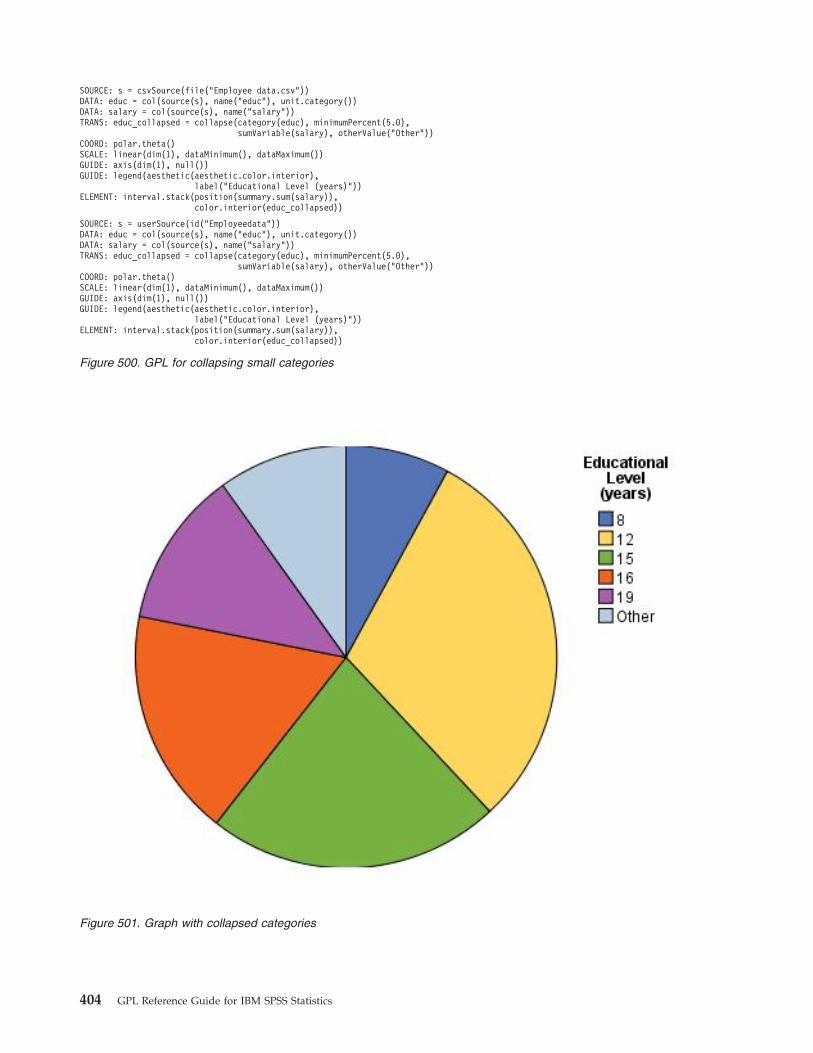
SOURCE: s = csvSource(file("Employee data.csv"))DATA: educ = col(source(s), name("educ"), unit.category())DATA: salary = col(source(s), name("salary"))TRANS: educ_collapsed = collapse(category(educ), minimumPercent(5.0),

sumVariable(salary), otherValue("Other"))COORD: polar.theta()SCALE: linear(dim(1), dataMinimum(), dataMaximum())GUIDE: axis(dim(1), null())GUIDE: legend(aesthetic(aesthetic.color.interior),

label("Educational Level (years)"))ELEMENT: interval.stack(position(summary.sum(salary)),

color.interior(educ_collapsed))

SOURCE: s = userSource(id("Employeedata"))DATA: educ = col(source(s), name("educ"), unit.category())DATA: salary = col(source(s), name("salary"))TRANS: educ_collapsed = collapse(category(educ), minimumPercent(5.0),

sumVariable(salary), otherValue("Other"))COORD: polar.theta()SCALE: linear(dim(1), dataMinimum(), dataMaximum())GUIDE: axis(dim(1), null())GUIDE: legend(aesthetic(aesthetic.color.interior),

label("Educational Level (years)"))ELEMENT: interval.stack(position(summary.sum(salary)),

color.interior(educ_collapsed))

Figure 500. GPL for collapsing small categories

Figure 501. Graph with collapsed categories


Mapping AestheticsThis example demonstrates how you can map a specific categorical value in the graph to a specificaesthetic value. In this case, "Female" bars are colored green in the resulting graph.

SOURCE: s = csvSource(file("Employee data.csv"))DATA: salary = col(source(s), name("salary"))DATA: jobcat = col(source(s), name("jobcat"), unit.category())DATA: gender = col(source(s), name("gender"), unit.category())COORD: rect(dim(1, 2), cluster(3))SCALE: cat(aesthetic(aesthetic.color), map(("Female", color.green)))GUIDE: axis(dim(2), label("Mean Salary"))GUIDE: axis(dim(3), label("Job Category"))ELEMENT: interval(position(summary.mean(gender*salary*jobcat)),

color(gender))

SOURCE: s = userSource(id("Employeedata"))DATA: salary = col(source(s), name("salary"))DATA: jobcat = col(source(s), name("jobcat"), unit.category())DATA: gender = col(source(s), name("gender"), unit.category())COORD: rect(dim(1, 2), cluster(3))SCALE: cat(aesthetic(aesthetic.color), map(("Female", color.green)))GUIDE: axis(dim(2), label("Mean Salary"))GUIDE: axis(dim(3), label("Job Category"))ELEMENT: interval(position(summary.mean(gender*salary*jobcat)),

color(gender))SCALE: cat(aesthetic(aesthetic.color), map(("f", color.green)))GUIDE: axis(dim(2), label("Mean Salary"))GUIDE: axis(dim(3), label("Job Category"))ELEMENT: interval(position(summary.mean(gender*salary*jobcat)),

color(gender))

Figure 502. GPL for mapping aesthetics

Figure 503. Graph with mapped aesthetics


Faceting by Separate VariablesThis example demonstrates how you can create facets based on separate variables, so that each facetshows the different variable information. Note that you can do something similar with nesting. See thetopic “Line Chart with Separate Scales” on page 384 for more information.

Grouping by Separate VariablesThis example demonstrates how you can create groups based on separate variables, so that each instanceof the graphic element shows the different variable information. In this example, you are comparing theresults of two variables across a categorical variable.

SOURCE: s = csvSource(file("Employee data.csv"))DATA: jobcat = col(source(s), name("jobcat"), unit.category())DATA: salary = col(source(s), name("salary"))DATA: salbegin = col(source(s), name("salbegin"))ELEMENT: schema(position(bin.quantile.letter(jobcat*salbegin*"Beginning Salary"+

jobcat*salary*"Current Salary")))

SOURCE: s = userSource(id("Employeedata"))DATA: jobcat = col(source(s), name("jobcat"), unit.category())DATA: salary = col(source(s), name("salary"))DATA: salbegin = col(source(s), name("salbegin"))ELEMENT: schema(position(bin.quantile.letter(jobcat*salbegin*"Beginning Salary"+

jobcat*salary*"Current Salary")))

Figure 504. GPL for faceting by separate variables

Figure 505. Faceting by separate variables


Clustering Separate VariablesThis example demonstrates how you can cluster separate variables.

SOURCE: s = csvSource(file("Employee data.csv"))DATA: salbegin=col(source(s), name("salbegin"))DATA: salary=col(source(s), name("salary"))DATA: educ=col(source(s), name("educ"), unit.category())GUIDE: axis(dim(1), label("Educational Level (years)"))ELEMENT: line(position(summary.mean(educ*salary)),color("Current Salary"))ELEMENT: line(position(summary.mean(educ*salbegin)),color("Beginning Salary"))

SOURCE: s = userSource(id("Employeedata"))DATA: salbegin=col(source(s), name("salbegin"))DATA: salary=col(source(s), name("salary"))DATA: educ=col(source(s), name("educ"), unit.category())GUIDE: axis(dim(1), label("Educational Level (years)"))ELEMENT: line(position(summary.mean(educ*salary)),color("Current Salary"))ELEMENT: line(position(summary.mean(educ*salbegin)),color("Beginning Salary"))

Figure 506. GPL for grouping by separate variables

Figure 507. Grouping by separate variables


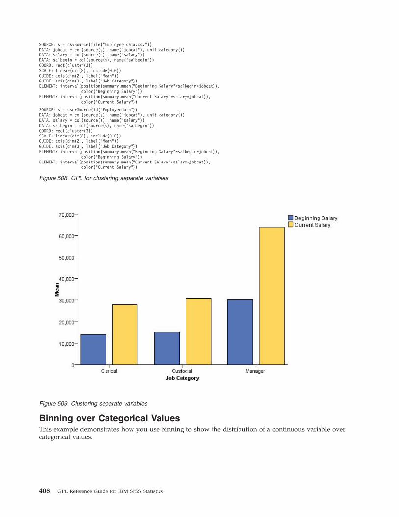
Binning over Categorical ValuesThis example demonstrates how you use binning to show the distribution of a continuous variable overcategorical values.

SOURCE: s = csvSource(file("Employee data.csv"))DATA: jobcat = col(source(s), name("jobcat"), unit.category())DATA: salary = col(source(s), name("salary"))DATA: salbegin = col(source(s), name("salbegin"))COORD: rect(cluster(3))SCALE: linear(dim(2), include(0.0))GUIDE: axis(dim(2), label("Mean"))GUIDE: axis(dim(3), label("Job Category"))ELEMENT: interval(position(summary.mean("Beginning Salary"*salbegin*jobcat)),

color("Beginning Salary"))ELEMENT: interval(position(summary.mean("Current Salary"*salary*jobcat)),

color("Current Salary"))

SOURCE: s = userSource(id("Employeedata"))DATA: jobcat = col(source(s), name("jobcat"), unit.category())DATA: salary = col(source(s), name("salary"))DATA: salbegin = col(source(s), name("salbegin"))COORD: rect(cluster(3))SCALE: linear(dim(2), include(0.0))GUIDE: axis(dim(2), label("Mean"))GUIDE: axis(dim(3), label("Job Category"))ELEMENT: interval(position(summary.mean("Beginning Salary"*salbegin*jobcat)),

color("Beginning Salary"))ELEMENT: interval(position(summary.mean("Current Salary"*salary*jobcat)),

color("Current Salary"))

Figure 508. GPL for clustering separate variables

Figure 509. Clustering separate variables


SOURCE: s = csvSource(file("Employee data.csv"))DATA: jobcat = col(source(s), name("jobcat"), unit.category())DATA: salary = col(source(s), name("salary"))GUIDE: axis(dim(1), label("Employment Category"))GUIDE: axis(dim(2), label("Current Salary"))GUIDE: legend(aesthetic(aesthetic.color), label("Count"))ELEMENT: polygon(position(bin.rect(jobcat*salary, dim(2))), color(summary.count()))

SOURCE: s = userSource(id("Employeedata"))DATA: jobcat = col(source(s), name("jobcat"), unit.category())DATA: salary = col(source(s), name("salary"))GUIDE: axis(dim(1), label("Employment Category"))GUIDE: axis(dim(2), label("Current Salary"))GUIDE: legend(aesthetic(aesthetic.color), label("Count"))ELEMENT: polygon(position(bin.rect(jobcat*salary, dim(2))), color(summary.count()))

Figure 510. GPL for binning over categorical values

Figure 511. Binning over categorical values


Categorical Heat Map

SOURCE: s = csvSource(file("Employee data.csv"))DATA: gender = col(source(s), name("gender"), unit.category())DATA: educ = col(source(s), name("educ"), unit.category())DATA: salary = col(source(s), name("salary"))GUIDE: axis(dim(1), label("Educational Level"))GUIDE: axis(dim(2), label("Gender"))GUIDE: legend(aesthetic(aesthetic.color), label("Mean Salary"))ELEMENT: point(position(educ*gender), shape(shape.square), size(size."10%"),

color(summary.mean(salary)))

SOURCE: s = userSource(id("Employeedata"))DATA: gender = col(source(s), name("gender"), unit.category())DATA: educ = col(source(s), name("educ"), unit.category())DATA: salary = col(source(s), name("salary"))GUIDE: axis(dim(1), label("Educational Level"))GUIDE: axis(dim(2), label("Gender"))GUIDE: legend(aesthetic(aesthetic.color), label("Mean Salary"))ELEMENT: point(position(educ*gender), shape(shape.square), size(size."10%"),

color(summary.mean(salary)))

Figure 512. GPL for categorical heat map

Figure 513. Categorical heat map


Creating Categories Using the eval FunctionThis example demonstrates how you can use the eval function to create categories based on anexpression.

SOURCE: s = csvSource(file("Employee data.csv"))DATA: gender = col(source(s), name("gender"), unit.category())DATA: educ = col(source(s), name("educ"), unit.category())DATA: salary = col(source(s), name("salary"))GUIDE: axis(dim(1), label("Educational Level"))GUIDE: axis(dim(2), label("Gender"))GUIDE: legend(aesthetic(aesthetic.color), label("Mean Salary"))ELEMENT: polygon(position(educ*gender), color(summary.mean(salary)))

SOURCE: s = userSource(id("Employeedata"))DATA: gender = col(source(s), name("gender"), unit.category())DATA: educ = col(source(s), name("educ"), unit.category())DATA: salary = col(source(s), name("salary"))GUIDE: axis(dim(1), label("Educational Level"))GUIDE: axis(dim(2), label("Gender"))GUIDE: legend(aesthetic(aesthetic.color), label("Mean Salary"))ELEMENT: polygon(position(educ*gender), color(summary.mean(salary)))

Figure 514. GPL for alternate categorical heat map

Figure 515. Alternate categorical heat map


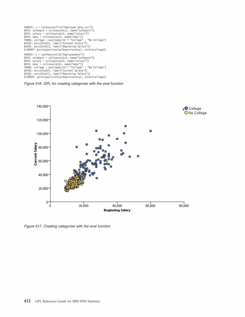
SOURCE: s = csvSource(file("Employee data.csv"))DATA: salbegin = col(source(s), name("salbegin"))DATA: salary = col(source(s), name("salary"))DATA: educ = col(source(s), name("educ"))TRANS: college = eval(educ>12 ? "College" : "No College")GUIDE: axis(dim(2), label("Current Salary"))GUIDE: axis(dim(1), label("Beginning Salary"))ELEMENT: point(position(salbegin*salary), color(college))

SOURCE: s = userSource(id("Employeedata"))DATA: salbegin = col(source(s), name("salbegin"))DATA: salary = col(source(s), name("salary"))DATA: educ = col(source(s), name("educ"))TRANS: college = eval(educ>12 ? "College" : "No College")GUIDE: axis(dim(2), label("Current Salary"))GUIDE: axis(dim(1), label("Beginning Salary"))ELEMENT: point(position(salbegin*salary), color(college))

Figure 516. GPL for creating categories with the eval function

Figure 517. Creating categories with the eval function


Chapter 4. GPL Constants

Color ConstantsColor constants: aliceblue, aqua, azure, bisque, black, blanchedalmond, blue, blueviolet, brown,burlywood, cadetblue, chartreuse, chocolate, coral, cornflowerblue, cornsilk, crimson, cyan, darkblue,darkcyan, darkgoldenrod, darkgray, darkgreen, darkgrey, darkkhaki, darkmagenta, darkolivegreen,darkorange, darkorchid, darkred, darksalmon, darkseagreen, darkslateblue, darkslategray, darkslategrey,darkturquoise, darkviolet, deeppink, deepskyblue, dimgray, dimgrey, dodgerblue, firebrick, floralwhite,forestgreen, fuchsia, gainsboro, ghostwhite, gold, goldenrod, gray, grey, green, greenyellow, honeydew,hotpink, indianred, indigo, ivory, khaki, lavender, lavenderblush, lawngreen, lemonchiffon, lightblue,lightcoral, lightcyan, lightgoldenrodyellow, lightgray, lightgreen, lightgrey, lightpink, lightsalmon,lightseagreen, lightskyblue, lightslategray, lightslategrey, lightsteelblue, lightyellow, lime, limegreen, linen,magenta, maroon, mediumaquamarine, mediumblue, mediumorchid, mediumpurple, mediumseagreen,mediumslateblue, mediumspringgreen, mediumturquoise, mediumvioletred, midnightblue, mintcream,mistyrose, moccasin, navajowhite, navy, oldlace, olive, olivedrab, orange, orangered, orchid,palegoldenrod, palegreen, paleturquoise, palevioletred, papayawhip, peachpuff, peru, pink, plum,powderblue, purple, red, rosybrown, royalblue, saddlebrown, salmon, sandybrown, seagreen, seashell,sienna, silver, skyblue, slateblue, slategray, slategrey, snow, springgreen, steelblue, tan, teal, thistle,tomato, turquoise, violet, wheat, white, whitesmoke, yellow, yellowgreen

Shape ConstantsThe following constants are all the valid constants for the different graphic element types. Note that theconstants for the edge graphic element appear in multiple tables.

shape.interior constants for interval elements: ibeam, line, square

shape.interior constants for edge and point elements: arrow, bowtie, circle, cross, decagon, elbow,elbowArrow, female, flower, flower3, flower4, flower5, flower6, flower7, flower8, flower9, flower10,heptagon, hexagon, hollowBowtie, hollowCircle, hollowDecagon, hollowHeptagon, hollowHexagon,hollowNonagon, hollowOctagon, hollowPentagon, hollowPolygon, hollowRoundRectangle, hollowSquare,hollowStar, hollowStar3, hollowStar4, hollowStar5, hollowStar6, hollowStar7, hollowStar8, hollowStar9,hollowStar10, hollowTriangle, ibeam, line, male, nonagon, octagon, pentagon, plus, polygon,roundRectangle, square, star, star3, star4, star5, star6, star7, star8, star9, star10, triangle

The following constants can also be used with the shape.exterior function to specify the border dashingof all other graphic elements. (An exception is the edge element, for which shape.interior defines theoverall shape or dashing.) These constants are also used with the shape function that specifies the dashingof form.line guides.

shape.interior constants for edge, line, and path elements: dash, dash_1_dot, dash_2_dots, dash_3_dots,dash_2x, dash_3x, dash_4_dots, dash_dash2x, half_dash, solid

Size ConstantsSize constants: tiny, small, medium, large, huge

Pattern ConstantsPattern constants: checkered, grid, grid2, grid3, grid4, grid5, mesh, mesh2, mesh3, mesh4, mesh5, pluses,pluses2, solid

413


Notices

This information was developed for products and services offered in the U.S.A.

IBM may not offer the products, services, or features discussed in this document in other countries.Consult your local IBM representative for information on the products and services currently available inyour area. Any reference to an IBM product, program, or service is not intended to state or imply thatonly that IBM product, program, or service may be used. Any functionally equivalent product, program,or service that does not infringe any IBM intellectual property right may be used instead. However, it isthe user's responsibility to evaluate and verify the operation of any non-IBM product, program, orservice.

IBM may have patents or pending patent applications covering subject matter described in thisdocument. The furnishing of this document does not grant you any license to these patents. You can sendlicense inquiries, in writing, to:

IBM Director of LicensingIBM CorporationNorth Castle DriveArmonk, NY 10504-1785U.S.A.

For license inquiries regarding double-byte (DBCS) information, contact the IBM Intellectual PropertyDepartment in your country or send inquiries, in writing, to:

Intellectual Property LicensingLegal and Intellectual Property LawIBM Japan Ltd.1623-14, Shimotsuruma, Yamato-shiKanagawa 242-8502 Japan

The following paragraph does not apply to the United Kingdom or any other country where suchprovisions are inconsistent with local law: INTERNATIONAL BUSINESS MACHINES CORPORATIONPROVIDES THIS PUBLICATION "AS IS" WITHOUT WARRANTY OF ANY KIND, EITHER EXPRESS ORIMPLIED, INCLUDING, BUT NOT LIMITED TO, THE IMPLIED WARRANTIES OFNON-INFRINGEMENT, MERCHANTABILITY OR FITNESS FOR A PARTICULAR PURPOSE. Somestates do not allow disclaimer of express or implied warranties in certain transactions, therefore, thisstatement may not apply to you.

This information could include technical inaccuracies or typographical errors. Changes are periodicallymade to the information herein; these changes will be incorporated in new editions of the publication.IBM may make improvements and/or changes in the product(s) and/or the program(s) described in thispublication at any time without notice.

Any references in this information to non-IBM Web sites are provided for convenience only and do not inany manner serve as an endorsement of those Web sites. The materials at those Web sites are not part ofthe materials for this IBM product and use of those Web sites is at your own risk.

IBM may use or distribute any of the information you supply in any way it believes appropriate withoutincurring any obligation to you.

415

Licensees of this program who wish to have information about it for the purpose of enabling: (i) theexchange of information between independently created programs and other programs (including thisone) and (ii) the mutual use of the information which has been exchanged, should contact:

IBM Software GroupATTN: Licensing200 W. Madison St.Chicago, IL; 60606U.S.A.

Such information may be available, subject to appropriate terms and conditions, including in some cases,payment of a fee.

The licensed program described in this document and all licensed material available for it are providedby IBM under terms of the IBM Customer Agreement, IBM International Program License Agreement orany equivalent agreement between us.

Any performance data contained herein was determined in a controlled environment. Therefore, theresults obtained in other operating environments may vary significantly. Some measurements may havebeen made on development-level systems and there is no guarantee that these measurements will be thesame on generally available systems. Furthermore, some measurements may have been estimated throughextrapolation. Actual results may vary. Users of this document should verify the applicable data for theirspecific environment.

Information concerning non-IBM products was obtained from the suppliers of those products, theirpublished announcements or other publicly available sources. IBM has not tested those products andcannot confirm the accuracy of performance, compatibility or any other claims related to non-IBMproducts. Questions on the capabilities of non-IBM products should be addressed to the suppliers ofthose products.

All statements regarding IBM's future direction or intent are subject to change or withdrawal withoutnotice, and represent goals and objectives only.

This information contains examples of data and reports used in daily business operations. To illustratethem as completely as possible, the examples include the names of individuals, companies, brands, andproducts. All of these names are fictitious and any similarity to the names and addresses used by anactual business enterprise is entirely coincidental.

COPYRIGHT LICENSE:

This information contains sample application programs in source language, which illustrate programmingtechniques on various operating platforms. You may copy, modify, and distribute these sample programsin any form without payment to IBM, for the purposes of developing, using, marketing or distributingapplication programs conforming to the application programming interface for the operating platform forwhich the sample programs are written. These examples have not been thoroughly tested under allconditions. IBM, therefore, cannot guarantee or imply reliability, serviceability, or function of theseprograms. The sample programs are provided "AS IS", without warranty of any kind. IBM shall not beliable for any damages arising out of your use of the sample programs.

Each copy or any portion of these sample programs or any derivative work, must include a copyrightnotice as follows:

© your company name) (year). Portions of this code are derived from IBM Corp. Sample Programs.

© Copyright IBM Corp. _enter the year or years_. All rights reserved.


TrademarksIBM, the IBM logo, and ibm.com are trademarks or registered trademarks of International BusinessMachines Corp., registered in many jurisdictions worldwide. Other product and service names might betrademarks of IBM or other companies. A current list of IBM trademarks is available on the Web at“Copyright and trademark information” at www.ibm.com/legal/copytrade.shtml.

Adobe, the Adobe logo, PostScript, and the PostScript logo are either registered trademarks or trademarksof Adobe Systems Incorporated in the United States, and/or other countries.

Intel, Intel logo, Intel Inside, Intel Inside logo, Intel Centrino, Intel Centrino logo, Celeron, Intel Xeon,Intel SpeedStep, Itanium, and Pentium are trademarks or registered trademarks of Intel Corporation or itssubsidiaries in the United States and other countries.

Linux is a registered trademark of Linus Torvalds in the United States, other countries, or both.

Microsoft, Windows, Windows NT, and the Windows logo are trademarks of Microsoft Corporation in theUnited States, other countries, or both.

UNIX is a registered trademark of The Open Group in the United States and other countries.

Java and all Java-based trademarks and logos are trademarks or registered trademarks of Oracle and/orits affiliates.

Notices 417

http://www.ibm.com/legal/copytrade.shtml


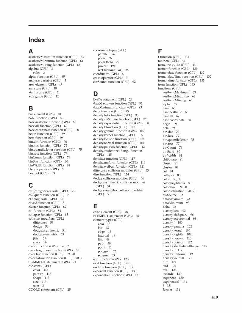
Index

AaestheticMaximum function (GPL) 63aestheticMinimum function (GPL) 64aestheticMissing function (GPL) 65algebra (GPL) 3

rules 3alpha function (GPL) 65analysis variable (GPL) 3area element (GPL) 47asn scale (GPL) 30atanh scale (GPL) 31axis guide (GPL) 42

Bbar element (GPL) 48base function (GPL) 66base.aesthetic function (GPL) 66base.all function (GPL) 67base.coordinate function (GPL) 68begin function (GPL) 69beta function (GPL) 69bin.dot function (GPL) 70bin.hex function (GPL) 72bin.quantile.letter function (GPL) 75bin.rect function (GPL) 77binCount function (GPL) 79binStart function (GPL) 80binWidth function (GPL) 81blend operator (GPL) 3boxplot (GPL) 53

Ccat (categorical) scale (GPL) 32chiSquare function (GPL) 81cLoglog scale (GPL) 32closed function (GPL) 81cluster function (GPL) 82col function (GPL) 84collapse function (GPL) 85collision modifiers (GPL)

difference 53dodge 54dodge.asymmetric 54dodge.symmetric 55jitter 55stack 56

color function (GPL) 86, 87color.brightness function (GPL) 88color.hue function (GPL) 89, 90color.saturation function (GPL) 90, 91COMMENT statement (GPL) 21constants (GPL)

color 413pattern 413shape 413size 413user 3

COORD statement (GPL) 25

coordinate types (GPL)parallel 26polar 26polar.theta 27project 194rect (rectangular) 28

coordinates (GPL) 6cross operator (GPL) 3csvSource function (GPL) 92

DDATA statement (GPL) 24dataMaximum function (GPL) 92dataMinimum function (GPL) 93delta function (GPL) 93density.beta function (GPL) 93density.chiSquare function (GPL) 96density.exponential function (GPL) 98density.f function (GPL) 100density.gamma function (GPL) 102density.kernel function (GPL) 105density.logistic function (GPL) 108density.normal function (GPL) 110density.poisson function (GPL) 112density.studentizedRange function

(GPL) 115density.t function (GPL) 117density.uniform function (GPL) 119density.weibull function (GPL) 121difference collision modifier (GPL) 53dim function (GPL) 124dodge collision modifier (GPL) 54dodge.asymmetric collision modifier

(GPL) 54dodge.symmetric collision modifier

(GPL) 55

Eedge element (GPL) 48ELEMENT statement (GPL) 46element types (GPL)

area 47bar 48edge 48interval 49line 49path 50point 51polygon 52schema 53

end function (GPL) 125eval function (GPL) 126exclude function (GPL) 130exponent function (GPL) 130exponential function (GPL) 131

Ff function (GPL) 131footnote (GPL) 44form.line guide (GPL) 43format function (GPL) 131format.date function (GPL) 132format.dateTime function (GPL) 132format.time function (GPL) 133from function (GPL) 133functions (GPL)

aestheticMaximum 63aestheticMinimum 64aestheticMissing 65alpha 65base 66base.aesthetic 66base.all 67base.coordinate 68begin 69beta 69bin.dot 70bin.hex 72bin.quantile.letter 75bin.rect 77binCount 79binStart 80binWidth 81chiSquare 81closed 81cluster 82col 84collapse 85color 86, 87color.brightness 88color.hue 89, 90color.saturation 90, 91csvSource 92dataMaximum 92dataMinimum 93delta 93density.beta 93density.chiSquare 96density.exponential 98density.f 100density.gamma 102density.kernel 105density.logistic 108density.normal 110density.poisson 112density.studentizedRange 115density.t 117density.uniform 119density.weibull 121dim 124end 125eval 126exclude 130exponent 130exponential 131f 131format 131

419

functions (GPL) (continued)format.date 132format.dateTime 132format.time 133from 133gamma 133gap 134gridlines 134in 135include 135index 136iter 136jump 136label 137, 138layout.circle 139layout.dag 141layout.data 143layout.grid 145layout.network 147layout.random 150layout.tree 152link.alpha 154link.complete 156link.delaunay 159link.distance 161link.gabriel 163link.hull 165link.influence 168link.join 170link.mst 172link.neighbor 175link.relativeNeighborhood 177link.sequence 179link.tsp 181logistic 183map 184marron 184max 185min 185mirror 186missing.gap 186missing.interpolate 187missing.listwise 187missing.pairwise 188missing.wings 188multiple 188noConstant 189node 189normal 190notIn 190opposite 190origin 191poisson 192position 192, 193preserveStraightLines 194proportion 195reflect 195region.confi.count 196region.confi.mean 198region.confi.percent.count 200region.confi.proportion.count 202region.confi.smooth 205region.spread.range 207region.spread.sd 209region.spread.se 212reverse 214root 215

functions (GPL) (continued)savSource 216scale 216, 217, 218scaledToData 218segments 219shape 219, 220showAll 221size 221, 222smooth.cubic 222smooth.linear 225smooth.loess 227smooth.mean 230smooth.median 232smooth.quadratic 235smooth.spline 237smooth.step 239sort.data 241sort.natural 241sort.statistic 242sort.values 242split 243sqlSource 243start 244startAngle 244studentizedRange 245summary.count 245summary.count.cumulative 247summary.countTrue 250summary.first 252summary.kurtosis 254summary.last 257summary.max 259summary.mean 261summary.median 263summary.min 265summary.mode 268summary.percent 270, 276summary.percent.count 271, 274summary.percent.sum 278, 281summary.percentile 283summary.percentTrue 285summary.proportion 288summary.proportion.count 289, 292summary.proportion.cumulative 294summary.proportion.sum 294, 297summary.proportionTrue 299summary.range 302summary.sd 304summary.se 306summary.se.kurtosis 308summary.se.skewness 311summary.sum 313summary.sum.cumulative 315summary.variance 317t 320texture.pattern 320tick 321to 321transparency 322, 323transpose 323uniform 324unit.percent 324userSource 324values 325visible 325weibull 326weight 326

functions (GPL) (continued)wrap 327

Ggamma function (GPL) 133gap function (GPL) 134GPL

algebra 3algebra and coordinate interaction 6algebra rules 3analysis variable 3blend operator 3clustering 17color constants 413constants, color 413constants, pattern 413constants, shape 413constants, size 413cross operator 3data sources for examples 329example data sources 329faceting 15introduction 1nest operator 3operator precedence 3operators 3paneling 15pattern constants 413shape constants 413size constants 413stacking 14syntax rules 3unity variable 3user constants 3using aesthetics 18

GRAPH statement (GPL) 22graphic element types (GPL)

area 47bar 48edge 48interval 49line 49path 50point 51polygon 52schema 53

graphic elements (GPL) 46gridlines function (GPL) 134GUIDE statement (GPL) 41guide types (GPL)

axis 42form.line 43legend 43line 43text.footnote 44text.subfootnote 44text.subsubfootnote 44text.subsubtitle 45text.subtitle 45text.title 45

Iin function (GPL) 135include function (GPL) 135


index function (GPL) 136interval element (GPL) 49iter function (GPL) 136

Jjitter collision modifier (GPL) 55jump function (GPL) 136

Llabel function (GPL) 137, 138layout.circle function (GPL) 139layout.dag function (GPL) 141layout.data function (GPL) 143layout.grid function (GPL) 145layout.network function (GPL) 147layout.random function (GPL) 150layout.tree function (GPL) 152legend guide (GPL) 43line element (GPL) 49line guide (GPL) 43linear scale (GPL) 34link.alpha function (GPL) 154link.complete function (GPL) 156link.delaunay function (GPL) 159link.distance function (GPL) 161link.gabriel function (GPL) 163link.hull function (GPL) 165link.influence function (GPL) 168link.join function (GPL) 170link.mst function (GPL) 172link.neighbor function (GPL) 175link.relativeNeighborhood function

(GPL) 177link.sequence function (GPL) 179link.tsp function (GPL) 181log scale (GPL) 34logistic function (GPL) 183logit scale (GPL) 35

Mmap function (GPL) 184marron function (GPL) 184max function (GPL) 185min function (GPL) 185mirror function (GPL) 186missing.gap function (GPL) 186missing.interpolate function (GPL) 187missing.listwise function (GPL) 187missing.pairwise function (GPL) 188missing.wings function (GPL) 188multiple function (GPL) 188

Nnest operator (GPL) 3noConstant function (GPL) 189node function (GPL) 189normal function (GPL) 190notIn function (GPL) 190

Ooperator precedence (GPL) 3operators (GPL) 3opposite function (GPL) 190origin function (GPL) 191

PPAGE statement (GPL) 22parallel coordinates (GPL) 26path element (GPL) 50point element (GPL) 51poisson function (GPL) 192polar coordinates (GPL) 26polar.theta coordinates (GPL) 27polygon element (GPL) 52position function (GPL) 192, 193pow scale (GPL) 36preserveStraightLines function

(GPL) 194prob scale (GPL) 37probit scale (GPL) 37project coordinates (GPL) 194proportion function (GPL) 195

Rrect (rectangular) coordinates (GPL) 28reference line (GPL) 43reflect function (GPL) 195region.confi.count function (GPL) 196region.confi.mean function (GPL) 198region.confi.percent.count function

(GPL) 200region.confi.proportion.count function

(GPL) 202region.confi.smooth function (GPL) 205region.spread.range function (GPL) 207region.spread.sd function (GPL) 209region.spread.se function (GPL) 212reverse function (GPL) 214root function (GPL) 215

SsafeLog scale (GPL) 38safePower scale (GPL) 39savSource function (GPL) 216scale function (GPL) 216, 217, 218SCALE statement (GPL) 29scale types (GPL) 30

asn 30atanh 31cat (categorical) 32cLoglog 32linear 34log 34logit 35pow 36prob 37probit 37safeLog 38safePower 39time 40

scaledToData function (GPL) 218

schema element (GPL) 53segments function (GPL) 219shape function (GPL) 219, 220showAll function (GPL) 221size function (GPL) 221, 222smooth.cubic function (GPL) 222smooth.linear function (GPL) 225smooth.loess function (GPL) 227smooth.mean function (GPL) 230smooth.median function (GPL) 232smooth.quadratic function (GPL) 235smooth.spline function (GPL) 237smooth.step function (GPL) 239sort.data function (GPL) 241sort.natural function (GPL) 241sort.statistic function (GPL) 242sort.values function (GPL) 242SOURCE statement (GPL) 23split function (GPL) 243sqlSource function (GPL) 243stack collision modifier (GPL) 56start function (GPL) 244startAngle function (GPL) 244statements (GPL) 21

COMMENT 21COORD 25DATA 24ELEMENT 46GRAPH 22GUIDE 41PAGE 22SCALE 29SOURCE 23TRANS 24

studentizedRange function (GPL) 245subfootnote guide (GPL) 44subsubfootnote guide (GPL) 44subsubtitle guide (GPL) 45subtitle guide (GPL) 45summary.count function (GPL) 245summary.count.cumulative function

(GPL) 247summary.countTrue function (GPL) 250summary.first function (GPL) 252summary.kurtosis function (GPL) 254summary.last function (GPL) 257summary.max function (GPL) 259summary.mean function (GPL) 261summary.median function (GPL) 263summary.min function (GPL) 265summary.mode function (GPL) 268summary.percent function (GPL) 270,

276summary.percent.count function

(GPL) 271, 274summary.percent.sum function

(GPL) 278, 281summary.percentile function (GPL) 283summary.percentTrue function

(GPL) 285summary.proportion function (GPL) 288summary.proportion.count function

(GPL) 289, 292summary.proportion.cumulative function

(GPL) 294summary.proportion.sum function

(GPL) 294, 297

Index 421

summary.proportionTrue function(GPL) 299

summary.range function (GPL) 302summary.sd function (GPL) 304summary.se function (GPL) 306summary.se.kurtosis function (GPL) 308summary.se.skewness function

(GPL) 311summary.sum function (GPL) 313, 315summary.variance function (GPL) 317syntax rules

GPL 3

Tt function (GPL) 320text.footnote guide (GPL) 44text.subfootnote guide (GPL) 44text.subsubfootnote guide (GPL) 44text.subsubtitle guide (GPL) 45text.subtitle guide (GPL) 45text.title guide (GPL) 45texture.pattern function (GPL) 320ticks function (GPL) 321time scale (GPL) 40title 2 (GPL) 45title 3 (GPL) 45title guide (GPL) 45to function (GPL) 321TRANS statement (GPL) 24transparency function (GPL) 322, 323transpose function (GPL) 323

Uuniform function (GPL) 324unit.percent function (GPL) 324unity variable (GPL) 3user constants (GPL) 3userSource function (GPL) 324

Vvalues function (GPL) 325visible function (GPL) 325

Wweibull function (GPL) 326Weibull scale (GPL) 32weight function (GPL) 326wrap function (GPL) 327


��

Printed in USA

Documents

GPL Reference Guide for IBM SPSS Statistics line in the example is a statement.One or more statements make up a block of GPL. Each statement specifies an aspect of the graph, such