Embed Size (px)
Citation preview

GPH: Similarity Search in Hamming SpaceJianbin Qin† Yaoshu Wang† Chuan Xiao‡ Wei Wang† Xuemin Lin† Yoshiharu Ishikawa‡
†University of New South Wales, Australia{jqin, yaoshuw, weiw, lxue}@cse.unsw.edu.au
‡ Nagoya University, [email protected] [email protected]
Abstract—A similarity search in Hamming space finds binaryvectors whose Hamming distances are no more than a thresholdfrom a query vector. It is a fundamental problem in manyapplications, including image retrieval, near-duplicate Web pagedetection, and machine learning. State-of-the-art approaches toanswering such queries are mainly based on the pigeonholeprinciple to generate a set of candidates and then verify them.
We observe that the constraint based on the pigeonhole prin-ciple is not always tight and hence may bring about unnecessarycandidates. We also observe that the distribution in real datais often skew, but most existing solutions adopt a simple equi-width partitioning and allocate the same threshold to all thepartitions, and hence fail to exploit the data skewness to optimizethe query processing. In this paper, we propose a new form ofthe pigeonhole principle which allows variable partition size andthreshold. Based on the new principle, we first develop a tightconstraint of candidates, and then devise cost-aware methodsfor dimension partitioning and threshold allocation to optimizequery processing. Our evaluation on datasets with various datadistributions shows the robustness of our solution and its superiorquery processing performance to the state-of-the-art methods.
I. INTRODUCTION
Finding similar objects is a fundamental problem in databaseresearch and has been studied for several decades [37]. Amongmany types of queries to find similar objects, Hamming distancesearch on binary vectors is an important one. Given a queryq, a Hamming distance search finds all vectors in a databasewhose Hamming distances to q are no greater than a thresholdτ . Answering such queries efficiently plays an important rolein many applications. In addition, it will receive increasinglyattention due to the continuous development and adoption ofdeep learning techniques.• Various forms of Hamming similarity search are fundamental
issues in computational geometry and theoretical computer sci-ence. For example, nearest neighbor [14] or range searches [9]can be reduced and solved in a Hamming cube using theHamming distance.
• Hamming similarity searches have been used in varioussimilarity search or retrieval applications. This is because onecan use various hashing techniques (either locality sensitivehashing [39] or metric-learning or deep-learning based learnedhash functions [38]) or manual feature exactions (e.g., inCheminformatics [40]) to obtain a compact binary code forobjects, and similarity search or retrieval can be performedefficiently in this Hamming cube.
We give several concrete and diverse application examples inthe following three areas:
• For image retrieval, images are converted to compact binaryvectors in traditional methods [34], [28]. Zhang et al. proposedto identify the vectors within a Hamming distance thresholdof 16 as candidates for further image-level verification [42].Recently, deep learning has become remarkably successful inimage recognition. Learning to hash algorithms that utilizeneural networks have been actively explored [17], [19], [7].In these studies, images are represented by binary vectorsand Hamming distance is utilized to capture the dissimilaritybetween images.
• To process text documents, state-of-the-art information retrievalmethods [29], [8] represent documents by binary vectorsthrough hashing. For Web page deduplication, Google usesSimHash to convert a Web page to a 64-bit vector, and thentwo pages are considered as near-duplicate if the Hammingdistance of the vectors are within 3 [22].
• For scientific databases, a fundamental task in cheminformaticsis to find similar molecules [12], [24]. In this task, moleculesare converted into binary vectors, and the Tanimoto similarityis used to measure the similarity between molecules. Thissimilarity constraint can be converted to an equivalentHamming distance constraint [43].
The naıve algorithm to answer a Hamming distance searchquery requires access and computation of every vector in thedatabase; hence it is expensive and does not scale well to largedatasets. Therefore, there has been much interest in devisingefficient indexes and algorithms. Many existing methods [1],[18], [43], [25] adopt the filter-and-refine framework to quicklyfind a set of candidates and then verify them. They are basedon the naıve application of the pigeonhole principle to thisproblem: If the n dimensions are partitioned into m equi-widthparts1, then a necessary condition for the Hamming distanceof two vectors to be within τ is that they must share a partin which the Hamming distance is within
⌊τm
⌋. This leads to
a filtering condition, and produces a set of candidate vectors,which are then verified by calculating the Hamming distancesand comparing with the threshold. As a result, the efficienciesof these methods critically depend on the candidate size.
However, despite the success and prevalence of this framework,we identify that the filtering condition has two inherent majorweaknesses: (1) The threshold on each partition is notalways tight. Hence, many unnecessary candidates are included.For example, when m = 3, the filtering conditions for τ in
1In this paper, we assume n mod m = 0.

0
0.2
0.4
0.6
0.8
1
0 20 40 60 80 100 120
Sk
ew
ness
Dimension
PubChemGIST
mSongTrevi3200
Ran50Cifar10
GloveRan100
Bigann2MNotreSIFT
UQVideo
FastText
Fig. 1. Skewness ( |#1s−#0s|#data
) by dimension of datasets in [16].
[9, 11] are the same (Hamming distance ≤⌊τm
⌋= 3), and hence
will produce the same set of candidates.(2) The thresholds on the partitions are evenly dis-
tributed. It assumes a uniform distribution and does not workwell when the dataset is skewed. We found that many realdatasets are skewed to varying degrees and complex correlationsexist among dimensions. Fig. 1 shows that 8 out of 11 realdatasets have dimensions with skewness greater than 0.3 2, and5 out of the 8 datasets contain a vector whose frequency ≥ 0.1on a partition, meaning that at least 1/10 data vectors becomecandidates if the query matches the data vector on this partition.
In this paper, we propose a novel method to answer theHamming distance search problem and address the above-mentioned weaknesses. We propose a tight form of the pigeonholeprinciple named general pigeonhole principle. Based on the newprinciple, the thresholds of the m partitions sum up to τ−m+1,less than τ , thus yielding a stricter filtering condition than theexisting methods. In addition, the threshold on each partition isa variable in the range of [−1, τ ], where −1 indicates that thispartition is ignored when generating candidates. This enablesus to choose proper thresholds for different partitions in orderto improve query processing performance. We prove that thecandidate condition based on the general pigeonhole principleis tight; i.e., the threshold allocated to each partition cannotbe further reduced. To tackle data skewness and dimensioncorrelations, we first devise an online algorithm to allocatethresholds to partitions using a query processing cost model, andthen devise an offline algorithm to optimize the partitioning ofvectors by taking account of the distribution of dimensions. Theproposed techniques constitute the GPH algorithm. Experimentsare run on several real datasets with different data distributions.The results show that the GPH algorithm performs consistentlywell on all these datasets and is faster than state-of-the-artmethods by up to two orders of magnitude.
Our contributions can be summarized as follows. (1) Wepropose a new form of the pigeonhole principle to obtain a tightfiltering condition and enable flexible threshold allocation. (2) Wepropose an efficient online query optimization method to allocatethresholds on the basis of the new pigeonhole principle. (3) Wepropose an offline partitioning method to address the selectivityissue caused by data skewness and dimension correlations. (4) We
2To measure the skewness of the i-th dimension, we calculate the numbersof vectors whose values on the i-th dimension are 0 and 1, respectively, andthen take the ratio of their difference and the total number of vectors.
conduct extensive experimental study on several real datasetsto evaluate the proposed method. The results demonstrate thesuperiority of the proposed method over state-of-the-art methods.
II. PRELIMINARIES
A. Problem Definition
In this paper, we focus on the similarity search on binaryvectors. We can view an object as an n-dimensional binaryvector x. x[i] denotes the value of the i-th dimension of x. Let∆(x[i], y[i]) = 0, if x[i] = y[i]; or 1, otherwise. The Hammingdistance between two vectors x and y, denoted H(x, y), is thenumber of dimensions on which x and y differ:
H(x, y) =
n∑i=1
∆(x[i], y[i]).
Hamming distance is a symmetric measure. If we regard x (re-spectively, y) as a yardstick, we can also say that y (respectively,x) has H(x, y) errors with respect to x (respectively, y).
Given a collection of data objects D, a query object q, aHamming distance search is to find all data objects whoseHamming distance to q is no greater than a threshold τ , i.e.,{x | x ∈ D, H(x, q) ≤ τ }.
B. Basic Pigeonhole Principle
Most exact solutions to Hamming distance search are basedon the filter-and-refine framework to generate a set of candidatesthat satisfy a necessary condition of the Hamming distanceconstraint. The majority of these methods [1], [18], [43], [25]are based on the intuition that if two vectors are similar, therewill be a pair of similar partitions from the two vectors. Hencethe (basic) pigeonhole principle is utilized by these methods.
Lemma 1 (Basic Pigeonhole Principle): x and y are di-vided into m partitions. Each partition consists of n
m dimensions.Let xi and yi (1 ≤ i ≤ m) denote each partition in x and y,respectively. If H(x, y) ≤ τ , there exists at least one partition isuch that H(xi, yi) ≤
⌊τm
⌋.
Any data object x satisfying the condition that ∃i, H(xi, qi) ≤⌊τm
⌋is called a candidate. Since these candidates will be verified
by computing the exact Hamming distance to the query, thequery processing performance depends heavily on the numberof candidates.
C. Overview of Existing Approaches
We briefly introduce a state-of-the-art method, Multi-indexHamming (MIH) [25]; other methods based on the basicpigeonhole principle work in a similar way. MIH partitions the ndimensions into m equi-width partitions. In each partition, basedon basic pigeonhole principle, it performs Hamming distancesearch on n′ =
⌊nm
⌋dimensions with a threshold τ ′ =
⌊τm
⌋.
MIH builds an inverted index offline, mapping each partition ofa data object to the object ID. For each partition of the query, itenumerates n′-dimensional vectors whose Hamming distances tothe partition are within τ ′. These vectors are called signatures.Then it looks up signatures in the index to find candidates andverifies them.
2

D. Weaknesses of Basic Pigeonhole Principle
Next we analyze the major drawbacks of the filtering conditionbased on the basic pigeonhole principle. Note that the filteringcondition is uniquely characterized by a vector of thresholdsallocated to each corresponding partition; we call the vectorthreshold vector, and denote the one used by the basic pigeonholeprinciple as Tbasic = [
⌊τm
⌋, . . . ,
⌊τm
⌋]. We also define the
dominance relationship between threshold vectors. Let ni denotethe number of dimensions in the i-th partition. T1 dominatesT2, or T1 ≺ T2, iff ∀i ∈ { 1, . . . ,m }, T1[i] ≤ T2[i] and[T1[i], T2[i]] ∩ [−1, ni − 1] 6= ∅, and ∃i, T1[i] < T2[i].• Tbasic is not always tight. By the tightness of a threshold
vector T , we mean that (1) (correctness) every vector whoseHamming distance to the query is within the thresholdwill be found by the filtering condition based on T , and(2) (minimality) there does not exists another vector T ′
that dominates T yet still guarantees correctness. As thecandidate size is monotonic with respect to the threshold, analgorithm based on a threshold vector which dominates Tbasicwill generate fewer or at most equal number of candidatescompared with an algorithm based on Tbasic.
Example 1: Consider τ = 9 and m = 3. The thresholdvector Tbasic is [3, 3, 3]. We can find a dominating thresholdvector T = [2, 2, 3] which is tight and guarantees bothcorrectness and minimality. Note that there may be multipletight threshold vectors for the same τ . E.g., another tightthreshold vector for the example can be [2, 3, 2] or [4, 3, 0] 3.
• The filtering condition does not adapt to the data distri-bution in the partitions. Skewness and correlations amongdimensions often exist in real data. Equal allocation ofthresholds, as done in Tbasic, may result in poor selectivityfor some partitions, hence excessive number of candidates.Several recent studies recognized this issue and proposedseveral methods to either obtain relatively less skew partitionsby partition rearrangement [43] or allocating varying thresholdsheuristically to different partitions [11]. In contrast, we proposethat skewed partitions can be beneficial and we can reduce thecandidate size by judiciously allocating different thresholds todifferent partitions for each query to exploit such skewness,as shown in Example 2.
Example 2: Suppose n = 8, m = 2, and τ = 2. Considerthe four data vectors and the query, and two differentpartitioning schemes in Table I. Consider the first query andexisting method will use Tbasic = [1, 1]. This will results in allthe four data vectors recognized as candidates, but only one(x1) is the result. If we use the first six dimensions as onepartition and the rest two dimensions as the other dimension,and use T = [2, 0], the candidate size will be reduced to 2(x1 and x2).
III. GENERAL PIGEONHOLE PRINCIPLE
In this section, we propose a general form of the pigeonholeprinciple which allows variable thresholds to guarantee thetightness of threshold vectors.
3Please refer to Section III for more explanation of tightness.
TABLE IBENEFITS OF ADAPTIVE PARTITIONING AND THRESHOLDING
Equi-width Partitioning Variable Partitioning
Partition 1 Partition 2 Partition 1 Partition 2
x1 = 00000000 0000 0000 000000 00x2 = 00000111 0000 0111 000001 11x3 = 00001111 0000 1111 000011 11x4 = 10011111 1001 1111 100111 11
q1 = 10000000 1000 0000 100000 00τ1 = 1 τ2 = 1 τ1 = 2 τ2 = 0
We begin with the allocation of thresholds. Given a thresholdvector, we use the notation ‖T‖1 to denote the sum of thresholdsin all the partitions, i.e., ‖T‖1 =
∑mi=1 T [i]. The flexible
pigeonhole principle is stated below.Lemma 2 (Flexible Pigeonhole Principle): A partitioning
P divides a n-dimensional vector into m disjoint partitions. xand y are partitioned by P . Consider a vector T = [τ1, . . . , τm]such that τi are integers and ‖T‖1 = τ . If H(x, y) ≤ τ , thereexists at least one partition i such that H(xi, yi) ≤ τi.
Proof: Assume that @i such that H(xi, yi) ≤ τi. Sincepartitions are disjoint, H(x, y) =
∑mi=1H(xi, yi) >
∑mi=1 τi.
Hence H(x, y) > τ , which contradicts that H(x, y) ≤ τ .The principle stated by Lemma 2 is more flexible than the
basic pigeonhole principle in the sense that we can choosearbitrary thresholds for different partitions. Intuitively, we maytolerate more errors for selective partitions and fewer errors forunselective partitions.
To achieve tightness, we first extend the threshold allocationfrom integers to real numbers.
Lemma 3: x and y are partitioned by P into m disjointpartitions. Consider a vector T = [τ1, . . . , τm] in which thethresholds are real numbers. ‖T‖1 = τ . If H(x, y) ≤ τ , thereexists at least one partition i such that H(xi, yi) ≤ bτic.
Proof: The proof of Lemma 2 also applies to real numbers.Therefore, if
∑mi=1 τi = τ and H(x, y) ≤ τ , then ∃i,
H(xi, yi) ≤ τi. Because τi are real numbers and H(xi, yi)are integers, ∃i, H(xi, yi) ≤ bτic.
Definition 1 (Integer Reduction): Given a threshold vec-tor T = [τ1, τ2, . . . , τm], we can reduce it to T ′ =[bτ1c , bτ2c , . . . , bτmc]. This reduction is called integer reduc-tion.
It is obvious that the candidate size does not change after aninteger reduction, as the Hamming distances must be integers.
When we combine Lemma 3 and the integer reductiontechnique, they can produce a threshold vector which dominatesTbasic, as shown in Example 3.
Example 3: Recall in Example 1, Tbasic is [3, 3, 3] using thebasic pigeonhole principle.
To obtain a dominating vector, we can start with a possiblethreshold vector T = [2.9, 2.9, 3.2]. Then by the integerreduction technique, T is reduced to T ′ = [2, 2, 3]. To see thisis correct, if 6 ∃i, H(xi, yi) ≤ T ′[i], there will be 3+3+4 = 10errors between x and y. Compared to [3, 3, 3], T ′ is a dominatingthreshold vector, and the constraints on the first two partitionsare stricter.
3
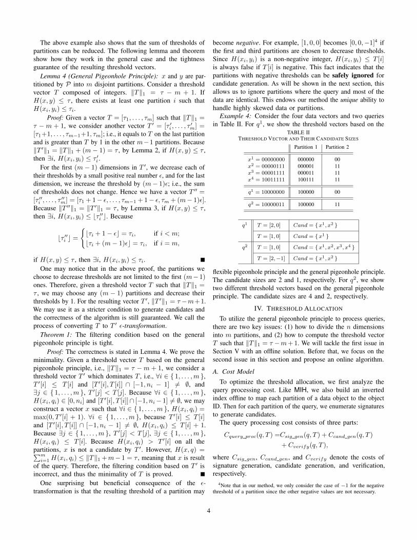
The above example also shows that the sum of thresholds ofpartitions can be reduced. The following lemma and theoremshow how they work in the general case and the tightnessguarantee of the resulting threshold vectors.
Lemma 4 (General Pigeonhole Principle): x and y are par-titioned by P into m disjoint partitions. Consider a thresholdvector T composed of integers. ‖T‖1 = τ − m + 1. IfH(x, y) ≤ τ , there exists at least one partition i such thatH(xi, yi) ≤ τi.
Proof: Given a vector T = [τ1, . . . , τm] such that ‖T‖1 =τ −m + 1, we consider another vector T ′ = [τ ′i , . . . , τ
′m] =
[τ1+1, . . . , τm−1+1, τm]; i.e., it equals to T on the last partitionand is greater than T by 1 in the other m−1 partitions. Because‖T ′‖1 = ‖T‖1 + (m− 1) = τ , by Lemma 2, if H(x, y) ≤ τ ,then ∃i, H(xi, yi) ≤ τ ′i .
For the first (m− 1) dimensions in T ′, we decrease each oftheir thresholds by a small positive real number ε, and for the lastdimension, we increase the threshold by (m− 1)ε; i.e., the sumof thresholds does not change. Hence we have a vector T ′′ =[τ ′′i , . . . , τ
′′m] = [τ1 + 1− ε, . . . , τm−1 + 1− ε, τm + (m− 1)ε].
Because ‖T ′′‖1 = ‖T ′‖1 = τ , by Lemma 3, if H(x, y) ≤ τ ,then ∃i, H(xi, yi) ≤ bτ ′′i c. Because
bτ ′′i c =
{bτi + 1− εc = τi, if i < m;
bτi + (m− 1)εc = τi, if i = m,
if H(x, y) ≤ τ , then ∃i, H(xi, yi) ≤ τi.One may notice that in the above proof, the partitions we
choose to decrease thresholds are not limited to the first (m−1)ones. Therefore, given a threshold vector T such that ‖T‖1 =τ , we may choose any (m − 1) partitions and decrease theirthresholds by 1. For the resulting vector T ′, ‖T ′‖1 = τ −m+1.We may use it as a stricter condition to generate candidates andthe correctness of the algorithm is still guaranteed. We call theprocess of converting T to T ′ ε-transformation.
Theorem 1: The filtering condition based on the generalpigeonhole principle is tight.
Proof: The correctness is stated in Lemma 4. We prove theminimality. Given a threshold vector T based on the generalpigeonhole principle, i.e., ‖T‖1 = τ −m + 1, we consider athreshold vector T ′ which dominates T , i.e., ∀i ∈ { 1, . . . ,m },T ′[i] ≤ T [i] and [T ′[i], T [i]] ∩ [−1, ni − 1] 6= ∅, and∃j ∈ { 1, . . . ,m }, T ′[j] < T [j]. Because ∀i ∈ { 1, . . . ,m },H(xi, qi) ∈ [0, ni] and [T ′[i], T [i]]∩ [−1, ni− 1] 6= ∅, we mayconstruct a vector x such that ∀i ∈ { 1, . . . ,m }, H(xi, qi) =max(0, T ′[i] + 1). ∀i ∈ { 1, . . . ,m }, because T ′[i] ≤ T [i]and [T ′[i], T [i]] ∩ [−1, ni − 1] 6= ∅, H(xi, qi) ≤ T [i] + 1.Because ∃j ∈ { 1, . . . ,m }, T ′[j] < T [j], ∃j ∈ { 1, . . . ,m },H(xi, qi) ≤ T [i]. Because H(xi, qi) > T ′[i] on all thepartitions, x is not a candidate by T ′. However, H(x, q) =∑mi=1H(xi, qi) ≤ ‖T‖1 +m− 1 = τ , meaning that x is result
of the query. Therefore, the filtering condition based on T ′ isincorrect, and thus the minimality of T is proved.
One surprising but beneficial consequence of the ε-transformation is that the resulting threshold of a partition may
become negative. For example, [1, 0, 0] becomes [0, 0,−1]4 ifthe first and third partitions are chosen to decrease thresholds.Since H(xi, yi) is a non-negative integer, H(xi, yi) ≤ T [i]is always false if T [i] is negative. This fact indicates that thepartitions with negative thresholds can be safely ignored forcandidate generation. As will be shown in the next section, thisallows us to ignore partitions where the query and most of thedata are identical. This endows our method the unique ability tohandle highly skewed data or partitions.
Example 4: Consider the four data vectors and two queriesin Table II. For q1, we show the threshold vectors based on the
TABLE IITHRESHOLD VECTOR AND THEIR CANDIDATE SIZES
Partition 1 Partition 2
x1 = 00000000 000000 00x2 = 00000111 000001 11x3 = 00001111 000011 11x4 = 10011111 100111 11
q1 = 10000000 100000 00
q2 = 10000011 100000 11
q1 T = [2, 0] Cand = {x1, x2 }
T = [1, 0] Cand = {x1 }
q2 T = [1, 0] Cand = {x1, x2, x3, x4 }
T = [2,−1] Cand = {x1, x2 }
flexible pigeonhole principle and the general pigeonhole principle.The candidate sizes are 2 and 1, respectively. For q2, we showtwo different threshold vectors based on the general pigeonholeprinciple. The candidate sizes are 4 and 2, respectively.
IV. THRESHOLD ALLOCATION
To utilize the general pigeonhole principle to process queries,there are two key issues: (1) how to divide the n dimensionsinto m partitions, and (2) how to compute the threshold vectorT such that ‖T‖1 = τ −m+ 1. We will tackle the first issue inSection V with an offline solution. Before that, we focus on thesecond issue in this section and propose an online algorithm.
A. Cost Model
To optimize the threshold allocation, we first analyze thequery processing cost. Like MIH, we also build an invertedindex offline to map each partition of a data object to the objectID. Then for each partition of the query, we enumerate signaturesto generate candidates.
The query processing cost consists of three parts:
Cquery proc(q, T ) =Csig gen(q, T ) + Ccand gen(q, T )
+ Cverify(q, T ),
where Csig gen, Ccand gen, and Cverify denote the costs ofsignature generation, candidate generation, and verification,respectively.
4Note that in our method, we only consider the case of −1 for the negativethreshold of a partition since the other negative values are not necessary.
4

For each partition i, a signature is a vector whose Hammingdistance is within τi to the i-th partition of query q. Since weenumerate all such vectors, the signature generation cost is
Csig gen(q, T ) =
m∑i=1
(niτi
)· cenum,
where ni denotes the number of dimensions in the i-th partition,and cenum is the cost of enumerating the value of a dimensionin a given vector. If τi < 0, the cost is 0 for the i-th partition.
Let Ssig denote the set of signatures generated. The candidategeneration cost can be modeled by inverted index lookup:
Ccand gen(q, T ) =∑s∈Ssig
|Is| · caccess,
where |Is| denotes the length of the postings list of signature s,and caccess is the cost of accessing an entry in a postings list.
The verification cost is
Cverify(q, T ) = |Scand| · cverify,
where Scand is the set of candidates, and cverify is the costto check if two n-dimensional vectors’ Hamming distance iswithin τ .
In practice, the signature generation cost is usually much lessthan the candidate generation cost and the verification cost (seeSection VII-B for experiments). So we can ignore the signaturegeneration cost when optimizing the threshold allocation. Inaddition, it is difficult to accurately estimate the size of Scandusing the lengths of postings lists, because it can be reducedfrom the minimal k-union problem [35], which is proved to beNP-hard. Nonetheless, |Scand| is upper-bounded by the sum ofcandidates generated in all the partitions, i.e.,
∑s∈Ssig |Is|. Our
experiments (Section VII-B) show that the ratio of |Scand| andthis upper bound depends on data distribution and τ . Given adataset, the ratio with respect to varying τ can be computed andrecorded by generating a number of queries and processing them.Let α denote this ratio. We may rewrite the number of candidatesin the form of α ·
∑mi=1 CN(qi, τi), where CN(qi, τi) is the
number of candidates generated by the i-th partition of the queryq with a threshold of τi (when τi = −1, CN(qi, τi) = 0).Hence the query processing cost can be estimated as:
Cquery proc(q, T ) =
m∑i=1
CN(qi, τi) · (caccess + α · cverify).
(1)
With the above cost model, we can formulate the thresholdallocation as an optimization problem.
Problem 1 (Threshold Allocation): Given a collection ofdata objects D, a query q and a threshold τ , find the thresholdvector T that minimizes the estimated query processing costunder the general pigeonhole principle; i.e.,
arg minT
Cquery proc(q, T ), s.t. ‖T‖1 = τ −m+ 1.
Algorithm 1: DPAllocate(q,m, τ)
1 for e = −1 to τ do2 OPT [1, e]← CN(q1, e), PATH[1, e]← e;
3 for i = 2 to m do4 for t = −i to τ − i+ 1 do5 cmin = +∞;6 for e = −1 to t+ i− 1 do7 if OPT [i− 1, t− e] + CN(qi, e) < cmin then8 cmin ← OPT [i− 1, t− e] + CN(qi, e);9 emin ← e;
10 OPT [i, t] = cmin, PATH[i, t] = emin;
11 e← τ −m+ 1;12 for i = m to 1 do13 T [i]← PATH[i, e];14 e← e− PATH[i, e];
15 return T ;
B. Threshold Allocation Algorithm
Since caccess, cverify , and α are independent of CN(qi, τi),we can omit the coefficient (caccess + α · cverify) in Equa-tion 1 and find the minimum query processing cost with onlyCN(qi, τi). The computation of CN(qi, τi) values will beintroduced in Section IV-C. Here we treat CN(qi, τi) as ablack box with O(1) time complexity and propose an onlinethreshold allocation algorithm based on dynamic programming.
Let OPT [i, t] record the minimum query processing cost(omitting the coefficient (caccess + α · cverify)) for partitions1, . . . , i with a sum of thresholds t. We have the followingrecursive formula:
OPT [i, t] =
t+i−1mine=−1
OPT [i− 1, t− e] + CN(qi, e),if i > 1;
CN(qi, t), if i = 1.
With the recursive formula, we design a dynamic programmingalgorithm for threshold allocation, whose pseudo-code is shownin Algorithm 1. It first initializes the costs for the first partition(Lines 1 – 2), i.e., OPT [1,−1], . . . , OPT [1, τ ]. Then it iteratesthrough the other partitions and compute the minimum costs(Lines 3 – 10). Note that the negative threshold −1 is alsoconsider for each partition. Finally, we trace the path that reachesOPT [m, τ −m+ 1] to obtain the threshold vector (Lines 11– 14). The time complexity of the algorithm is O(m · (τ + 1)2).
Example 5: Consider a dataset of 100 binary vectors and wepartition it into 4 partitions. Given a query q, for each partitioni, suppose the numbers of candidates (denoted CNi) underdifferent thresholds are provided in the table below.
τi = −1 τi = 0 τi = 1 τi = 2 τi = 3 τi = 4
CN1 0 5 10 15 50 100CN2 0 10 80 90 95 100CN3 0 5 15 20 70 100CN4 0 10 70 80 95 100
We use Algorithm 1 to compute the threshold vector. TheOPT [i, t] values are given in the table below.
5

t = i = 1 i = 2 i = 3 i = 4
-3 0 0 0 5-2 0 0 5 10-1 0 5 10 200 5 15 20 301 10 20 20 302 15 25 35 453 50 60 40 454 100 110 45 55
The minimum query processing cost OPT [4, 4] = 55. Wetrace the path (in boldface) that reaches this value and obtainthe threshold vector [2, 0, 2, 0].
C. Computing Candidate Numbers
In order to run the threshold allocation algorithms, we need toobtain the candidate numbers CN(qi, τi) beforehand. An exactsolution to computing CN(qi, τi) is to enumerate all possiblevectors for the i-th partition and then count how many vectors inD has a Hamming distance within τi to the enumerated vectorin this partition. These numbers are stored in a table. Whenprocessing the query, with the given qi, the table is looked upfor the corresponding entry CN(qi, τi). The time complexityof this algorithm is O(m · 2n · 2τ ), and the space complexityis O(m · 2n). This method is only feasible when n and τ aresmall. To cope with large n and τ , we devise two approximationalgorithms to estimate the number of candidates.
Sub-partitioning. The basic idea of the first approximationalgorithm is splitting qi into smaller equi-width sub-partitionsand estimating CN(qi, τi) with the candidate numbers of thesub-partitions. We divide qi into mi sub-partitions. Each sub-partition has a fixed number of dimensions so that its candidatenumber can be computed using the exact algorithm in reasonableamount of time and stored in main memory. For the thresholds ofthe sub-partitions, we may use the general pigeonhole principleand divide τi into mi values such that they sum up to τi−mi+1.Let qij denote a sub-partition of qi and τij denote its threshold.Let G(mi, τi) be the set of threshold vectors of which thetotal thresholds sum up to no more than τi − mi + 1; i.e.,{ [τi1, . . . , τimi ]|τij ∈ [−1, τi] ∧
∑mij=1 τij ≤ τi −mi + 1 }.
We offline compute all the CN(qij , τij) values for all τij ∈[−1, τi] using the aforementioned exact algorithm; i.e., enumerateall possible query vectors and then count how many data vectorsin D has a Hamming distance within τij to the enumeratedvector in this sub-partition. We assume that the candidates inthe mi sub-partitions are independent. Then CN(qi, τi) can beapproximately estimated online with the following equation.
CN(qi, τi) =∑
g∈G(mi,τi)
mi∏j=1
(CN(qij , g[j])− CN(qij , g[j]− 1)).
Machine Learning. We may also use machine learningtechnique to predict the candidate number for a given 〈qi, τi〉.For each τi, we regard each dimension of qi as a feature andrandomly generate feature vectors xk = [b1, . . . , b|qi|]. Thecandidate number CN(xk, τi) can be obtained by processing
xk as a query with a threshold τi. Then we apply the regressionmodel on the training data Ti = { 〈xk, CN(xk, τi)〉 }.
Let hτi(xi, θi) denote the machine learning model, whereθi denotes its parameters. Traditional regression models utilizemean squared error as loss function. To reduce the impact oflarge CN(xk, τi), we use relative error as our loss function:J(Ti, θi) =
∑|Ti|k=1{
CN(xk,τi)−hτi (xk,θi)CN(xk,τi)
}2. According to [27],we utilize the approximation ln(t) ≈ t−1 to estimate J(Ti, θi):
J(Ti, θi) =
|Ti|∑k=1
{1− hτi(xk, θi)
CN(xk, τi)
}2
≈|Ti|∑i=1
{lnCN(xk, τi)
hτi(xk, θi)
}2
=
|Ti|∑i=1
{lnCN(xk, τi)− lnhτi(xk, θi)}2.
From the above equation, we can simply convert training data〈xk, CN(xk, τi)〉 into 〈xk, lnCN(xk, τi)〉 and then take meansquared error to train an SVM model with RBF kernel.
V. DIMENSION PARTITIONING
To deal with data skewness and dimension correlations, theexisting methods for Hamming distance search resort to randomshuffle [1] or dimension rearrangement [43], [36], [20]. Allof them are aiming towards the direction that the dimensionsin each partition or the signatures in the index are uniformlydistributed, so as to reduce the candidates caused by frequentsignatures. In this section, we present our method for dimensionpartitioning. We devise a cost model of dimension partitioningand convert the partitioning into an optimization problem tooptimize query processing performance. Then we propose thealgorithm to solve this problem.
A. Cost Model
Let Pi denote a set of dimensions in the range [1, n]. Ourgoal is to find a partitioning P = {P1, . . . , Pm } such thatPi∩Pj = ∅ if i 6= j, and ∪mi=1Pi = { 1, . . . , n }. Given a queryworkload Q = {< q1, τ1 >, . . . , < q|Q|, τ |Q| > }, the queryprocessing cost of the workload is the sum of the costs of itsconstituent queries:
Cworkload(Q,P) =
|Q|∑i=1
Cquery proc(qi, τ i,P), (2)
where Cquery proc(qi, τ i,P) is the processing cost of query
qi with a threshold τ i, which can be computed using the dynamicprogramming algorithm proposed in Section IV. Then we canformulate the dimension partitioning as an optimization problem.
Problem 2 (Dimension Partitioning): Given a collection ofdata objects D, a query workload Q, find the partitioning Pthat minimizes the query processing cost of Q under the generalpigeonhole principle; i.e.,
arg minP
Cworkload(Q,P).
6

Lemma 5: The dimension partitioning problem is NP-hard.Proof: We can reduce the dimension partitioning problem
from the number partitioning problem [2], which is to partitiona multiset of positive integers, S, into two subsets S1 andS2 such that the difference between the sums in two sets isminimized. Consider a special case of m = 2 and a Q ofonly one query. Let S be a multiset of n positive integers,each representing a dimension in the dimension partitioningproblem. Let sum(S) denote the sum of numbers in S. Fori ∈ { 1, 2 }, Let CN(qi, τi) = sum(Si)
2, ∀τi ∈ [−1, τ ]; i.e.,the candidate number in partition i equals to the square ofthe sum of numbers in this partition. By Equations 1 and 2,Cworkload(Q,P) = (sum(S1)2 + sum(S2)2) · (caccess + α ·cverify). Cworkload is minimized when the difference betweensum(S1) and sum(S2) is minimized. Hence the special caseof dimension partitioning problem is reduced from the numberpartitioning problem. Because the number partitioning problemis NP-complete, the dimension partitioning is NP-hard.
B. Partitioning Algorithm
Seeing the difficulty of the dimension partitioning problem,we propose a heuristic algorithm to select a good partitioning:first generate an initial partitioning and then refine it.
Algorithm 2 captures the pseudo-code of the heuristicpartitioning algorithm. It first generates an initial partitioning Pof m partitions (Line 1). The details of the initialization stepwill be introduced in Section V-C. Then the algorithm iterativelyimproves the current partitioning by selecting the best optionof moving a dimension from one partition to another. In eachiteration, we pick a dimension from a partition Pi (Line 8), tryto move it to another partition Pj , j 6= i (Line 10), and computethe resulting query processing cost of the workload. We try allpossible combination of Pi and Pj , and the option that yieldsthe minimum cost is taken as the move of this iteration (Line 16).The above steps repeat until the cost cannot be further improvedby moving a dimension. The time complexity of the algorithm isO(lmnc). l is the number of iterations. c is the time complexityof computing the cost of the workload, O(|Q| ·m ·(τ+1)2). Wealso note that due to the replacement of dimensions, partitionsmay become empty in our algorithm. Hence it is not mandatoryto output exactly m partitions for an input partition number m.
For the input query workload Q, in case a historical queryworkload is unavailable, a sample of data objects can be used asa surrogate. Our experiments show that even if the distributionof real queries are different from the query workload that we useto compute the partitioning, our query processing algorithm stillachieves good performance (Section VII-G). We also note thatwe may assign varying thresholds to the queries in the workloadQ. The benefit is that we can offline compute the partitioningusing the workload which cover a wide range of thresholds, andthen build an index without being aware of the thresholds ofreal queries beforehand.
C. Initial Partitioning
Since the dimension partitioning algorithm stops at a localoptimum, we may achieve a better result with a carefully
Algorithm 2: HeuristicPartition(D,Q,m)
1 P ← InitialPartition(D,Q,m);2 cmin ← Cworkload(Q,P);3 f ← true;4 while f = true do5 f ← false;6 foreach Pi ∈ P do7 foreach d ∈ Pi do8 P ′i ← Pi \ { d }, P ′ ← (P \ Pi) ∪ P ′i ;9 foreach Pj ∈ P, j 6= i do
10 P ′j ← Pj ∪ { d }, P ′ ← (P ′ \ Pj) ∪ P ′j ;11 if Cworkload(Q,P ′) < cmin then12 f ← true;13 cmin ← Cworkload(Q,P ′);14 Pmin ← P ′;
15 if f = true then16 P ← Pmin;
17 return P;
selected initial partitioning. The correlation of dimensions playan important role here. Unlike the existing methods which tryto make dimensions in each partition uniformly distributed, ourmethod aims at the opposite direction. We observe that the queryprocessing performance is usually improved if highly correlateddimensions are put into the same partitions. This is because ourthreshold allocation algorithm works online and optimizes eachquery individually. When highly correlated dimensions are puttogether, more errors are likely to be identified in a partition,and thus our threshold allocation algorithm can assign a largerthreshold to this partition and smaller thresholds to the otherpartitions; i.e., choosing proper thresholds for different partitions.If the dimensions are uniformly distributed, all the partitions willhave the same distribution and there is little chance to optimizefor specific partitions.
We may measure the correlation of dimensions with entropy.For a partition Pi, we project all the data objects in D on thedimensions of Pi, and use DPi to denote the set of the resultingvectors. The correlation of the dimensions of Pi is measured by:
H(DPi) = −∑
X∈DPi
P (X) · logP (X).
According to the definition of entropy, a smaller value ofentropy indicates a higher correlation of the dimensions of Pi.The entropy of the partitioning P is the sum of the entropies ofits constituent partitions:
H(P) =
m∑i=1
H(DPi).
Our goal is to find an initial partitioning P to minimize H(P).To achieve this, we generate an equi-width partitioning in agreedy manner: Starting with an empty partition, we select thedimension which yields the smallest entropy if it is put intothis partition. This is repeated until a fixed partition size
⌊nm
⌋is reached, and thereby the first partition is obtained. Then we
7

repeat the above procedure on the unselected dimensions togenerate the other (m− 1) partitions.
VI. THE GPH ALGORITHM
Based on the general pigeonhole principle and the techniquesproposed in Sections IV and V, we devise the GPH (short forthe General Pigeonhole principle-based algorithm for Hammingdistance search) algorithm.
The GPH algorithm consists of two phases: indexing phaseand query processing phase. In the indexing phase, it takesas input the dataset D, the query workload Q, and a tunableparameter m for the number of partitions. The partitioning Pis generated using the heuristic partitioning algorithm proposedin Section V. Then for each n-dimensional vector x in D, wedivided it by P into m partitions. Then for the projection ofx on each partition, the ID of vector x is inserted into thepostings list of this projection. In the query processing phase,the query q and the threshold τ are input to the algorithm. Itfirst partitions q by P into m partitions. Then the thresholdvector T is computed using the dynamic programming algorithmproposed in Section IV. For the projection of q on each partition,we enumerate the signatures whose Hamming distances to theprojection do not exceed the allocated threshold. Then for eachsignature, we probe the inverted index to find the data objectsthat have this signature in the same partition, and insert thevector IDs into the candidate set. The candidates are finallyverified using Hamming distance and the true results are returned.We omit the pseudo-code here in the interest of space.
We note that in case of a query service level agreement, withthe data and query workloads provided by the user, we are ableto estimate the query response time of GPH using the costreturned by the threshold allocation algorithm. Then we caneither guarantee the number of queries that can be handled in aspecific amount of time using current computing resources, orlet the user know the amount of additional resources required toprocess the queries.
VII. EXPERIMENTS
We report experiment results and analyses in this section.
A. Experiments Setup
The following algorithms are compared in the experiment.• MIH is a method based on the basic pigeonhole principle [25].
It divides vectors into m equi-width partitions and uses athreshold
⌊τm
⌋on all the partitions to generate candidates.
Its filtering condition is not tight. Signatures are enumeratedon the query side. We utilize the open source of MIH onGitHub 5 and chose the fastest m setting on each dataset.
• HmSearch is a method based on the basic pigeonholeprinciple [43]. Vectors are divided into
⌊τ+32
⌋equi-width
partitions. It has a filtering condition in multiple cases but nottight. The threshold of a partition is either 0 or 1. This is oneof our previous work and we utilize the existing source code.
• PartAlloc is a method to solve the set similarity joinproblem [11]. It divides vectors into τ+1 equi-width partitions5https://github.com/norouzi/mih
and allocate thresholds to partitions with three options: −1,0, and 1. −1 means that the partition is disregarded forcandidate generation. Its filtering condition is tight. Signaturesare enumerated on both data and query vectors. The sourcecode is received from the authors of [11]. We convert theHamming distance constraint to an equivalent Jaccard similarityconstraint [1], which is supported by the source code. Thegreedy method [11] is chosen to allocate thresholds. Positionalfilters (checking the number of dimensions whose values are1 in each partition and discarding a candidate if the differenceexceeds τ ) have already been implemented in the providedsource code and are invoked when generating candidates.
• LSH is an algorithm to retrieve approximate answers. Weconvert the Hamming distance constraint to an equivalentJaccard similarity constraint and then use the minhash LSH [5].The dimension which yields the minimum hash value is chosenas a minhash. k minhashes are concatenated into a singlesignature, and this is repeated l times to obtain l signatures. Weset k to 3 and recall to 95%. l =
⌈log1−tk(1− r)
⌉, where t is
the Jaccard similarity threshold. The algorithm is implementedby ourselves.
• GPH is the method proposed in this paper. We implement iton top of the source code of MIH for fair comparison.Other methods for Hamming distance search, e.g., [18], [15],
[22], are not compared since prior work [43] showed they areoutperformed by HmSearch. We do not consider the methodin [30] because it focuses on small n (≤ 64) and small τ (≤ 4),and it is significantly slower than the other algorithms in ourexperiments. E.g., on GIST, when τ = 8, its average queryresponse time is 128 times longer than GPH. The approximatemethod proposed in [26] is only fast for small thresholds. OnSIFT, when τ ≥ 12, it becomes slower than MIH even if therecall is set to 0.9 [26]. Due to its performance compared toMIH and the much larger threshold settings in our experiments,we do not compare with the method in [26].
We select five publicly available real datasets with differentdata distributions and application domains.• SIFT is a set of 1 billion SIFT features from the BIGANN
dataset 6 [13]. We follow the method used in [25] to convertthem into 128-dimensional binary vectors.
• GIST is a set of 80 million 256-dimensional GIST descriptorsfor tiny images 7 [33].
• PubChem is a database of chemical molecules 8. We sample1 million entries, each of which is a 881-dimensional vector.
• FastText is a set of 1 million English word vectors trainedon Wikipedia 2017 9. We convert them into binary vectors of128 dimensions by spectral hashing [39].
• UQVideo is a set of 3.3 million keyframes of Web videosfrom the UQ Video project 10. Each keyframe is convertedto a binary vector of 256 dimensions by multiple featurehashing [31].
6http://corpus-texmex.irisa.fr/7http://horatio.cs.nyu.edu/mit/tiny/data/index.html8https://pubchem.ncbi.nlm.nih.gov/9https://fasttext.cc/docs/en/english-vectors.html10http://staff.itee.uq.edu.au/shenht/UQ VIDEO/
8

0.01
0.1
1
10
100
1000
10000
6 12 18 24 30
Av
g.
Qu
ery
Tim
e (m
s)
Threshold
verification
S
S
S
SS
candidate generationsignature enumeration
threshold allocation
0.01
0.1
1
10
100
1000
10000
6 12 18 24 30
Av
g.
Qu
ery
Tim
e (m
s)
Threshold
GG
GG
G
0.01
0.1
1
10
100
1000
10000
6 12 18 24 30
Av
g.
Qu
ery
Tim
e (m
s)
Threshold
P
PP
PP
(a) Response Time Decomposed
1000
10000
100000
1x10⁶
1x10⁷
1x10⁸
4 8 12 16 20 24 28 32
Can
d v
s.
Su
m
Threshold
SIFT-sum
SIFT-cand
GIST-sum
GIST-cand
PubChem-sum
PubChem-cand
(b) Compare∑s∈Ssig
|Is| and Scand
Fig. 2. Justification of Assumptions
SIFT has the smallest skewness among the five. GIST andUQVideo are medium skewed datasets. PubChem and FastTextare highly skewed datasets. In addition to the five real datasets,we generate a synthetic dataset with varying skewness.
We sample a subset of 100 vectors from each dataset asthe query workload for the partitioning of GPH. To generatereal queries, for each dataset we sample 1,000 vectors (differfrom the query workload for partitioning) and take the rest asdata objects. We vary τ and measure the query response timeaveraged over 1,000 queries. For GPH and PartAlloc, thresholdallocation time are also included. The τ settings are up to 32,64, 32, 20, and 48 on the five real datasets, respectively. Thereason why we set smaller thresholds on PubChem is that dueto the skewness, more than 10% data objects are results whenτ = 32.
The experiments are carried out on a server with a Quad-Core Intel Xeon E3-1231 @3.4GHz Processor and 96GB RAM,running Debian 6.0. All the algorithms are implemented in C++in a main memory fashion.
B. Justification of Assumptions
We first justify our assumptions for the cost model of thresholdallocation. Fig. 2(a) shows the query processing time of GPH onSIFT, GIST, and PubChem (denoted S, G, and P, respectively).The time is decomposed into four parts: threshold allocation,signature enumeration, candidate generation, and verification.The figure is plotted in logscale so that threshold allocationand signature enumeration can be seen. Compared to candidategeneration and verification, the time spent on threshold allocationand signature enumeration is negligible (< 3%), meaning thatwe can ignore them when estimating the query processingcost. Fig. 2(b) shows the sum of candidates generated inall the partitions (
∑s∈Ssig |Is|, denoted dataset-sum) and
the candidate sizes (|Scand|, denoted dataset-cand) on thethree datasets. It can be seen that |Scand| is upper-boundedby∑s∈Ssig |Is|. The ratio of them varies from 0.69 to 0.98,
depending on dataset and τ . The ratios on different datasets andτ settings are recorded as the value of α in Equation 1 for costestimation.
C. Evaluation of Threshold Allocation
We evaluate threshold allocation by comparing with a baselinealgorithm (denoted RR). RR allocates thresholds in a round robinmanner, and the thresholds of all partitions sum up to τ −m+1.For a fair comparison, we randomly shuffle the dimensions andthen use the equi-width partitioning (m is chosen for the best
1x10⁶
1x10⁷
1x10⁸
4 8 12 16 20 24 28 32
Av
g.
Est
imat
ed C
ost
Threshold
RR DP
(a) SIFT, Allocation Method, Cost
100
1000
10000
4 8 12 16 20 24 28 32
Av
g.
Qu
ery
Tim
e (m
s)
Threshold
RR DP
(b) SIFT, Allocation Method, Time
10000
100000
1x10⁶
1x10⁷
1x10⁸
8 16 24 32 40 48 56 64
Av
g.
Est
imat
ed C
ost
Threshold
RR DP
(c) GIST, Allocation Method, Cost
10
100
1000
8 16 24 32 40 48 56 64
Av
g.
Qu
ery
Tim
e (m
s)
Threshold
RR DP
(d) GIST, Allocation Method, Time
10000
100000
1x10⁶
1x10⁷
4 8 12 16 20 24 28 32
Av
g.
Est
imat
ed C
ost
Threshold
RR DP
(e) PubChem, Allocation Method, Cost
1
10
100
4 8 12 16 20 24 28 32
Av
g.
Qu
ery
Tim
e (m
s)
Threshold
RR DP
(f) PubChem, Allocation Method, Time
Fig. 3. Evaluation of Threshold Allocation
performance) for the competitors in this set of experiments.Figs. 3(a), 3(c), and 3(e) show the query processing costs (interms of candidate numbers) estimated by DP on SIFT, GIST,and PubChem. We also plot the costs of RR using our costmodel. The corresponding query response times are shown inFigs. 3(b), 3(d), and 3(f). The trends of the cost and the timeare similar, indicating that the cost model effectively estimatesthe query processing performance. DP is significantly faster thanRR in query processing, and the gap is more remarkable ondatasets with more skewness. On PubChem, the time of RRis close to sequential scan due to the skewness. With judiciousthreshold allocation, the time is reduced by nearly two ordersof magnitude.
To evaluate the candidate number computation, we comparethe sub-partitioning algorithm (denoted SP) and the machinelearning algorithm based on SVM model (denoted SVM). Toshow why we choose SVM as the machine learning model, wealso compare with two other learning models: random forest(RF) and a 3-layer deep neural network (DNN). The number ofsub-partitions is 2. The size of the training data is 1,000 for themachine learning algorithms. Table III shows the relative errorswith respect to the exact method and the times of candidatenumber computation (in microseconds). Since the performanceson the real datasets are similar, we only show the results onthe GIST dataset. The relative error of SVM is very small, andit is more accurate and faster than SP. To compare learningmodels, the relative error of RF is much higher than the othermethods. Although DNN estimates candidate numbers slightlymore accurately than SVM in some settings, their relative errorsare both very small, and the running time of DNN is much morethan SVM. In addition, we tried logistic regression and gradientboosting decision tree. Their relative errors are higher than theabove methods and hence not shown here. Seeing these results,
9

100
1000
10000
4 8 12 16 20 24 28 32
Av
g.
Qu
ery
Tim
e (m
s)
Threshold
GR
OR
OS
DD
RS
(a) SIFT, Partitioning Method, Time
100
1000
10000
4 8 12 16 20 24 28 32
Av
g.
Qu
ery
Tim
e (m
s)
Skewness
GreedyInitOriginalInit
RandomInit
(b) SIFT, Initial Partitioning, Time
10
100
1000
8 16 24 32 40 48 56 64
Av
g.
Qu
ery
Tim
e (m
s)
Threshold
GR
OR
OS
DD
RS
(c) GIST, Partitioning Method, Time
10
100
1000
8 16 24 32 40 48 56 64
Av
g.
Qu
ery
Tim
e (m
s)
Skewness
GreedyInitOriginalInit
RandomInit
(d) GIST, Initial Partitioning, Time
1
10
100
4 8 12 16 20 24 28 32
Av
g.
Qu
ery
Tim
e (m
s)
Threshold
GR
OR
OS
DD
RS
(e) PubChem, Partitioning Method, Time
1
10
4 8 12 16 20 24 28 32
Av
g.
Qu
ery
Tim
e (m
s)
Skewness
GreedyInitOriginalInit
RandomInit
(f) PubChem, Initial Partitioning, Time
Fig. 4. Evaluation of Dimension Partitioning
we choose the machine learning algorithm based on SVM modelto estimate candidate numbers in the rest of the experiments.
TABLE IIIESTIMATION WITH VARIOUS MODELS ON GIST (EACH CELL SHOWSPERCENTAGE ERROR AND PREDICTION TIME (µS), SEPARATED BY /)
τ SP SVM RF DNN
16 1.75%/0.47 1.64%/0.31 8.73%/0.40 1.78%/2.6432 0.37%/0.77 0.28%/0.28 12.43%/0.39 0.19%/2.6048 0.15%/2.67 0.10%/0.43 9.26%/0.73 0.08%/3.8364 0.07%/3.45 0.06%/0.29 3.58%/0.44 0.03%/2.44
D. Evaluation of Dimension Partitioning
To evaluate the effect of partitioning, we compare our method(denoted GR) with the following competitors: (1) OR is to usethe original unshuffled order of the dataset. (2) RS is to performa random shuffle on the original order. (3) OS [43] and DD [36]are two dimension rearrangement methods to make dimensionsin each partition uniformly distributed. We run GPH with theabove partitioning methods and show the query response timesin Figs. 4(a), 4(c), and 4(e). On SIFT, their performances areclose. When the dataset has more skewness, the advantage ofGR becomes remarkable. It is faster than the runner-up by upto 4 times on GIST and 8 times on PubChem.
To evaluate the effect of initial partitioning, we run ourpartitioning algorithm with three initial states: (1) the proposedmethod which tries to minimize entropy (denoted GreedyInit),(2) equi-width partitioning on the original unshuffled data(denoted OriginalInit), and (3) equi-width partitioning afterrandom shuffle (denoted RandomInit). The corresponding queryresponse times on the three datasets are plotted in Figs. 4(b), 4(d),and 4(f). The trends are similar to the previous set of experiments.On datasets with more skewness, GreedyInit is consistently
100
1000
10000
4 8 12 16 20 24 28 32
Av
g.
Qu
ery
Tim
e (m
s)
Threshold
m=6
m=8
m=10
m=12
m=14
(a) SIFT, Effect of m, Time
10
100
1000
8 16 24 32 40 48 56 64
Av
g.
Qu
ery
Tim
e (m
s)
Threshold
m=10
m=12
m=14
m=16
m=18
(b) GIST, Effect of m, Time
1
10
4 8 12 16 20 24 28 32
Av
g.
Qu
ery
Tim
e (m
s)
Threshold
m=38
m=44
m=50
m=56
m=62
(c) PubChem, Effect of m, Time
Fig. 5. Effect of Partition Number
faster than the other competitors, and the gap to the runner-upcan be up to 2 times.
As for the query workload Q to compute dimension parti-tioning, our results show that the effect of its size on the queryprocessing performance is not obvious.E.g., when τ = 64, theaverage query processing times vary from 4.19 to 3.97 secondson GIST, if we increase |Q| from 100 to 1000. Thus we choose100 as the size of Q in our experiments.
We also study the effect of partition number on the queryprocessing performance. Figs. 5(a) – 5(c) show the queryresponse times on SIFT, GIST, and PubChem by varyingthe number of partitions. The general trend is that a smaller mperforms better under small τ settings. When τ increases, the bestchoice of m slightly increases. The reason is: (1) When τ is small,a small m is good enough. Dividing vectors into unnecessarilylarge number of partitions yields very small partitions and henceincreases the frequency of signatures. (2) When τ is large, asmall m means more thresholds will be allocated to a partition,and this results in more candidates. Hence a slightly larger m isbetter in this case. Based on the results, we suggest user choosem ≈ n
24 for GPH for good query processing performance.
E. Comparison with Existing Methods
We compare GPH with alternative methods (equipped withthe OS partitioning [43]) for Hamming distance search.
Index are compared first. Figs. 6(a) – 6(e) show the indexsizes of the algorithms on the five datasets. LSH, HmSearch,and PartAlloc run out of memory for some τ settings on SIFTand GIST. We only show the points when the memory canhold their indexes. GPH consume more space than MIH dueto the machine learning-based technique to estimate candidatenumbers. Both algorithms consume less space than the otherexact competitors. This is expected as GPH and MIH enumeratesignatures on query vectors only. HmSearch and PartAllocenumerate 1-deletion variants on data vectors; i.e., removingan arbitrary dimension from a partition and taking the rest asa signature. The variants are indexed and this will increasetheir index sizes. PartAlloc and LSH exhibit variable indexsizes with respect to τ . LSH has the smallest index size onPubChem, but consumes much more space on the other datasets.
10

15000
30000
60000
4 8 12 16 20 24 28 32
Ind
ex
Siz
e (
MB
)
Threshold
GPH
MIH
PartAlloc
LSH
(a) SIFT, Index Size
2500
5000
10000
20000
40000
80000
8 16 24 32 40 48 56 64
Ind
ex
Siz
e (
MB
)
Threshold
GPH
MIH
HmSearch
PartAlloc
LSH
(b) GIST, Index Size
3
12
48
192
768
4 8 12 16 20 24 28 32
Ind
ex
Siz
e (
MB
)
Threshold
GPH
MIH
HmSearch
PartAlloc
LSH
(c) PubChem, Index Size
100
1000
4 6 8 10 12 14 16 18 20
Ind
ex
Siz
e (
MB
)
Threshold
GPH
MIH
HmSearch
PartAlloc
LSH
(d) FastText, Index Size
1000
10000
4 8 12 16 20 24 28 32 36 40 44 48
Ind
ex
Siz
e (
MB
)
Threshold
GPH
MIH
HmSearch
PartAlloc
LSH
(e) UQVideo, Index Size
Fig. 6. Comparison with Alternatives - Index Size
TABLE IVINDEX CONSTRUCTION TIME ON GIST (S)
τ MIH HmSearch PartAlloc LSH GPH
16 481 1681 1736 583 5026 + 56032 481 1689 3244 5221 5026 + 56048 481 1711 7600 64256 5026 + 56064 481 1747 9605 N/A 5026 + 560
The reason is that PubChem has much more dimensions thanthe other datasets. Hence given a τ , the equivalent Jaccardthreshold is higher on PubChem, resulting in less number ofsignatures. The corresponding index construction times on GISTare shown in Table IV. LSH runs out of memory when τ = 64,and thus is shown for the other τ settings. The time of GPHis decomposed into dimension partitioning and indexing. MIHspends the least amount of time on index construction. Despitemore time consumption on partitioning, GPH spends less timeindexing data objects than the other algorithms. We argue thatthe partitioning can be done offline and the time is affordable.Because the query workload Q for partitioning computationconsists of queries with varying thresholds, we can run thepartitioning once and use the same partitioning for different τsettings in real queries. This is also the reason why GPH hasconstant partitioning and indexing time irrespective of τ .
The candidate numbers are plotted in Figs. 7(a), 7(c), 7(e),7(g), and 7(i). The corresponding query response times are plottedin Figs. 7(b), 7(d), 7(f), 7(h), and 7(j). For all the algorithms,candidate numbers and running times increase when τ movestowards larger values, and their trends are similar. Thanks tothe tight filtering condition and cost-aware partitioning andthreshold allocation, GPH is consistently smaller than MIH andHmSearch in candidate size and faster than the two methods.The only exception is that HmSearch has smaller candidate
size when τ = 4 on PubChem and τ ≤ 8 on UQVideo, butturns out to be slower than GPH. This is because HmSearchgenerates many signatures whose postings lists are empty, andthis drastically increases signature enumeration and index lookuptimes. Although PartAlloc has a tight filtering condition andutilizes threshold allocation, it is not as fast as GPH, andeven slower than MIH. This result showcases that PartAlloc’spartitioning and threshold allocation is not efficient for Hammingdistance search, though it pays off on set similarity search.Another interesting observation is that LSH does not performwell on highly skewed data. The reason is that the hash functionsmay choose highly skewed and correlated dimensions, and thusthe selectively of the chosen signatures becomes very bad. OnPubChem, LSH’s performance is close to a sequential scan.Overall, GPH is the fastest algorithm. The speed-ups against therunner-up algorithms on the five datasets are up to 22, 21, 135,32, and 8 times, respectively. We also notice that when τ ≥ 16on FastText, the speed-up of GPH against MIH becomes lessremarkable. This is because more than 59% data objects areresults, meaning that both MIH and GPH are ineffective infiltering. Nonetheless, GPH is faster than MIH by 1.3 times, andboth methods are significantly faster than the other competitors.
F. Varying Number of Dimensions
We compare the five competitors to evaluate their performanceswhen varying the number of dimensions. We sample 25%, 50%,75%, and 100% dimensions from SIFT, GIST, and PubChem,and then run the experiment. τ = 12, 24, and 12 for the 100%sample on the three datasets, respectively, and we let τ changelinearly with the number of sampled dimensions. Figs. 8(a)– 8(c) show the query response times of the algorithms on thethree datasets. We observe that the times of all the algorithmsincrease with n. There are two factors: (1) Although τ and nincrease proportionally, the number of results increases with ndue to dimension correlations. Hence we have more candidatesto verify. (2) The verification cost increases with n becausemore dimensions are compared. Nonetheless, GPH is alwaysthe fastest algorithm among the competitors, especially on themore skewed PubChem.
G. Varying Skewness
We study the performance by varying skewness 11. As seenfrom Fig. 1, the relationship between skewness and dimensionsis approximately linear (except PubChem) on most datasets. Onthe basis of this observation, the synthetic dataset is generated asfollows: The number of dimensions is 128. The mean skewnessis controlled by a parameter γ, and the skewnesses of the 128dimensions range from 0 to 2γ. We set τ = 12. The queryprocessing times are plotted in Fig. 8(d). The general trend isthat all the algorithms become slower on more skewed data. Thisis expected as signatures become less selective. Nonetheless,thanks to variable partitioning and threshold allocation, GPH isthe fastest among the five competitors.
To demonstrate the robustness of GPH, we show that even ifthe distribution of real queries is different from the sample to
11See the footnote in Section I for the measurement of dataset skewness.
11

100000
1x10⁶
1x10⁷
1x10⁸
4 8 12 16 20 24 28 32
Av
g.
Can
did
ate
Siz
e
Threshold
GPH
MIH
PartAlloc
LSH
(a) SIFT, Candidate Number
100
1000
10000
4 8 12 16 20 24 28 32
Av
g.
Qu
ery
Tim
e (m
s)
Threshold
GPH
MIH
PartAlloc
LSH
(b) SIFT, Query Processing Time
10000
100000
1x10⁶
1x10⁷
8 16 24 32 40 48 56 64
Av
g.
Can
did
ate
Siz
e
Threshold
GPH
MIH
HmSearch
PartAlloc
LSH
(c) GIST, Candidate Number
10
100
1000
10000
8 16 24 32 40 48 56 64
Av
g.
Qu
ery
Tim
e (m
s)
Threshold
GPH
MIH
HmSearch
PartAlloc
LSH
(d) GIST, Query Processing Time
1000
10000
100000
1x10⁶
4 8 12 16 20 24 28 32
Av
g.
Can
did
ate
Siz
e
Threshold
GPH
MIH
HmSearch
PartAlloc
LSH
(e) PubChem, Candidate Number
1
10
100
4 8 12 16 20 24 28 32
Av
g.
Qu
ery
Tim
e (m
s)
Threshold
GPH
MIH
HmSearch
PartAlloc
LSH
(f) PubChem, Query Processing Time
10000
100000
1x10⁶
4 6 8 10 12 14 16 18 20
Av
g.
Can
did
ate
Nu
mb
er
Threshold
GPH
MIH
HmSearch
PartAlloc
LSH
(g) FastText, Candidate Number
1
10
100
4 6 8 10 12 14 16 18 20
Qu
ery
Tim
e (m
s)
Threshold
GPH
MIH
HmSearch
PartAlloc
LSH
(h) FastText, Query Processing Time
100
1000
10000
100000
1x10⁶
4 8 12 16 20 24 28 32 36 40 44 48
Av
g.
Can
did
ate
Nu
mb
er
Threshold
GPH
MIH
HmSearch
PartAlloc
LSH
(i) UQVideo, Candidate Number
1
10
100
1000
4 8 12 16 20 24 28 32 36 40 44 48
Qu
ery
Tim
e (m
s)
Threshold
GPH
MIH
HmSearch
PartAlloc
LSH
(j) UQVideo, Query Processing Time
Fig. 7. Comparison with Alternatives - Candidate Number & Time
compute partitioning, our method retains good performance. Wegenerate a synthetic dataset with a γ of 0.5, and then computepartitioning with two query workloads: γ = 0.5 (denoted GPH-0.5) and γ = 0.1 (denoted GPH-0.1), respectively. Then we runa set of queries with a γ of 0.1. The gap between GPH-0.5and GPH-0.1 can be regarded as the extent to which GPH’sperformance deteriorates in the presence of a different querydistribution. Then we set γ to 0.1 for the synthetic dataset andrun the experiment again. Results are plotted in Figs. 8(e) – 8(f).It can be seen that although GPH computes partitioning witha workload whose distribution is different from real queries,the query processing performance is almost the same. A slightdifference can be noticed only when τ is as large as 12, where thequery processing speed drops by 11.1% and 4.4%, respectively.
VIII. RELATED WORK
The notion of Hamming distance search was first proposedin [23]. Due to its wide range of applications, the problem hasreceived considerable attention in the last few decades.
100
1000
10000
32 64 96 128
Av
g.
Qu
ery
Tim
e (m
s)
Dimension
GPH
MIH
PartAlloc
(a) SIFT, Effect of n, Time
10
100
1000
10000
64 128 192 256
Av
g.
Qu
ery
Tim
e (m
s)
Dimension
GPH
MIH
HmSearch
PartAlloc
LSH
(b) GIST, Effect of n, Time
1
10
100
1000
220 440 660 880
Av
g.
Qu
ery
Tim
e (m
s)
Dimension
GPH
MIH
HmSearch
PartAlloc
LSH
(c) PubChem, Effect of n, Time
0.1
1
10
100
0.1 0.2 0.3 0.4 0.5
Av
g.
Qu
ery
Tim
e (m
s)
γ
GPH
MIH
HmSearch
PartAlloc
LSH
(d) Synthetic, Effect of Skewness, Time
0.1
0.2
0.3
0.4
0.5
0.6
0.7
0.8
0.9
1
3 6 9 12
Av
g.
Qu
ery
Tim
e (m
s)
Threshold
GPH-0.1 GPH-0.5
(e) Synthetic, γD = 0.5, γq = 0.1,Time
0.2
0.4
0.6
0.8
1
1.2
3 6 9 12
Av
g.
Qu
ery
Tim
e (m
s)
Threshold
GPH-0.1 GPH-0.5
(f) Synthetic, γD = 0.1, γq = 0.5,Time
Fig. 8. Varying Number of Dimensions and Skewness
A few studies focused on the special case when τ = 1 [3],[4], [21], [41]. Among them, the method by [21] indexes allthe 1-variants of the data vectors to answer the query in O(1)time and O(
(nτ
)) space. A data structure was proposed in [4] to
answer this special case in O(1) time using O(n logm) spaceby a cell probe model with word size m.
For the general case of Hamming distance search, the methodby [10] is able to answer Hamming distance search in O(m+logτ (nm) +occ) time and O(n logτ (nm)) space, where occ isthe number of results. In practice, many solutions are based onthe pigeonhole principle to convert the problem to sub-problemswith a threshold τ ′, where τ ′ < τ . In [32], [18], [25], vectorsare divided into a number of partitions such that query resultsmust have at least one exact match with the query in one of thepartitions. The idea of recursive partitioning was covered in [22].Before that, a two-level partitioning idea was adopted by thePartEnum method [1]. Song et al. [30] proposed to enumeratethe combinations within threshold τ ′ in each partition to avoidthe verification of candidates. Ong and Bober [26] proposed anapproximate method utilizing variable length hash keys. In [43],vectors are divided into
⌊τ+32
⌋partitions, and the threshold of
a partition can be either 0 or 1. Deng et al. [11] also proposedto use different thresholds on partitions, and the thresholds arecomputed by the allocation algorithm. We briefly discuss thedifferences from our method: (1) The method in [11] targetsthe set similarity join problem. Although it can be convertedto Hamming distance searches, the number of dimensions arelarge (usually > 10000) and the vectors are sparse (usually< 1000 non-zero values), which are different from the datasetsin most applications of Hamming distance search. (2) Equi-width partitioning is used in [11], and the number of partitionsis τ + 1. In GPH, we use variable partition size and the number
12

of partitions is a tunable parameter m. (3) For the thresholdson partitions, there are three options in [11]: 0, 1, and skipped(equivalent to −1 in GPH). We do not have this limitation, andthe thresholds may vary from −1 to τ . (4) To find candidates,signature enumerations are performed on both data and queryvectors in [11], whereas we only enumerate on queries.
To handle the poor selectivity caused by data skewnessand dimension correlations, existing work mainly focused ontwo strategies. The first is to perform a random shuffle [1]in original dimensions to avoid highly correlated dimensionsin same partitions. The second is to perform a dimensionrearrangement [43], [36], [20] to minimize the correlationbetween dimensions in each partition. These methods are ableto answer queries efficiently on slightly skewed datasets, but theperformances deteriorate on highly skewed datasets.
We note that a strong form of the pigeonhole principle wasintroduced in [6] which states that given n positive integersq1, . . . , qm, if (
∑mi=1 qi−m+ 1) objects are distributed into m
boxes, then either the first box contains at least q1 objects, . . .,or the n-th box contains at least qn objects. Although the generalpigeonhole principle proposed in this paper coincides with theabove strong form, by integer reduction and ε-transformation, thegeneral pigeonhole principle is not limited to positive integers(this is the reason why GPH performs well on skewed data) andthe tightness of threshold allocation is proved, hence providinga deeper understanding of the pigeonhole principle.
IX. CONCLUSION AND FUTURE WORK
In this paper, we proposed a new approach to similaritysearch in Hamming space. Observing the major drawbacksof the basic pigeonhole principle adopted by many existingmethods, we developed a new form of the pigeonhole principle,based on which the condition of candidate generation is tight.The cost of query processing was modeled, and then anoffline dimension partitioning algorithm and an online thresholdallocation algorithm were devised on top of the model. Weconducted experiments on real datasets with various distributions,and showed that our approach performs consistently well on allthese datasets and outperforms state-of-the-art methods.
Our future work includes extending general pigeonholeprinciple to other similarity constraints. Another direction is toexplore the techniques to dealing with the parallel case.
Acknowledgements. J. Qin, Y. Wang, and W. Wang arepartially supported by ARC DP170103710, and D2DCRCDC25002 and DC25003. C. Xiao and Y. Ishikawa are supportedby JSPS Kakenhi 16H01722. X. Lin is supported by NSFC61672235, ARC DP170101628 and DP180103096. We thankthe authors of [11] for kindly providing their source codes.
REFERENCES
[1] A. Arasu, V. Ganti, and R. Kaushik. Efficient exact set-similarity joins. InVLDB, 2006.
[2] J. M. Borwein and D. H. Bailey. Mathematics by experiment - plausiblereasoning in the 21st century. A K Peters, 2003.
[3] G. S. Brodal and L. Gasieniec. Approximate dictionary queries. In CPM,pages 65–74, 1996.
[4] G. S. Brodal and S. Venkatesh. Improved bounds for dictionary look-upwith one error. Inf. Process. Lett., 75(1-2):57–59, 2000.
[5] A. Z. Broder. On the resemblance and containment of documents. InSEQS, 1997.
[6] R. Brualdi. Introductory Combinatorics. Math Classics. Pearson, 2017.[7] Z. Cao, M. Long, J. Wang, and P. S. Yu. Hashnet: Deep learning to hash
by continuation. In ICCV, pages 5609–5618, 2017.[8] S. Chaidaroon and Y. Fang. Variational deep semantic hashing for text
documents. In SIGIR Conference, pages 75–84, 2017.[9] B. Chazelle, D. Liu, and A. Magen. Approximate range searching in
higher dimension. Comput. Geom., 39(1):24–29, 2008.[10] R. Cole, L.-A. Gottlieb, and M. Lewenstein. Dictionary matching and
indexing with errors and don’t cares. In STOC, pages 91–100, 2004.[11] D. Deng, G. Li, H. Wen, and J. Feng. An efficient partition based method
for exact set similarity joins. PVLDB, 9(4):360–371, 2015.[12] D. R. Flower. On the properties of bit string-based measures of chemical
similarity. Journal of Chemical Information and Computer Sciences,38(3):379–386, 1998.
[13] H. Jegou, R. Tavenard, M. Douze, and L. Amsaleg. Searching in onebillion vectors: re-rank with source coding. CoRR, abs/1102.3828, 2011.
[14] E. Kushilevitz, R. Ostrovsky, and Y. Rabani. Efficient search forapproximate nearest neighbor in high dimensional spaces. In Proceedingsof the Thirtieth Annual ACM Symposium on Theory of Computing, STOC’98, pages 614–623, New York, NY, USA, 1998. ACM.
[15] C. Li, J. Lu, and Y. Lu. Efficient merging and filtering algorithms forapproximate string searches. In ICDE, 2008.
[16] W. Li, Y. Zhang, Y. Sun, W. Wang, W. Zhang, and X. Lin. Approximatenearest neighbor search on high dimensional data - experiments, analyses,and improvement (v1.0). CoRR, abs/1610.02455, 2016.
[17] K. Lin, H. Yang, J. Hsiao, and C. Chen. Deep learning of binary hashcodes for fast image retrieval. In CVPR Workshops, pages 27–35, 2015.
[18] A. X. Liu, K. Shen, and E. Torng. Large scale hamming distance queryprocessing. In ICDE, pages 553–564, 2011.
[19] H. Liu, R. Wang, S. Shan, and X. Chen. Deep supervised hashing for fastimage retrieval. In CVPR Conference, pages 2064–2072, 2016.
[20] Y. Ma, H. Zou, H. Xie, and Q. Su. Fast search with data-oriented multi-index hashing for multimedia data. TIIS, 9(7):2599–2613, 2015.
[21] U. Manber and S. Wu. An algorithm for approximate membership checkingwith application to password security. Inf. Process. Lett., 50(4):191–197,1994.
[22] G. S. Manku, A. Jain, and A. D. Sarma. Detecting near-duplicates forweb crawling. In WWW, pages 141–150, 2007.
[23] M. Minsky and S. Papert. Perceptrons - an introduction to computationalgeometry. MIT Press, 1987.
[24] R. Nasr, R. Vernica, C. Li, and P. Baldi. Speeding up chemical searchesusing the inverted index: The convergence of chemoinformatics and textsearch methods. J. Chem. Inf. Model, 2012.
[25] M. Norouzi, A. Punjani, and D. J. Fleet. Fast search in hamming spacewith multi-index hashing. In CVPR, pages 3108–3115, 2012.
[26] E. Ong and M. Bober. Improved hamming distance search using variablelength hashing. In CVPR Conference, pages 2000–2008, 2016.
[27] H. Park and L. Stefanski. Relative-error prediction. Statistics & ProbabilityLetters, 40(3):227 – 236, 1998.
[28] M. Raginsky and S. Lazebnik. Locality-sensitive binary codes fromshift-invariant kernels. In NIPS Conference, pages 1509–1517, 2009.
[29] R. Salakhutdinov and G. E. Hinton. Semantic hashing. Int. J. Approx.Reasoning, 50(7):969–978, 2009.
[30] J. Song, H. T. Shen, J. Wang, Z. Huang, N. Sebe, and J. Wang. Adistance-computation-free search scheme for binary code databases. IEEETrans. Multimedia, 18(3):484–495, 2016.
[31] J. Song, Y. Yang, Z. Huang, H. T. Shen, and R. Hong. Multiplefeature hashing for real-time large scale near-duplicate video retrieval. InProceedings of the 19th ACM International Conference on Multimedia,MM ’11, pages 423–432, New York, NY, USA, 2011. ACM.
[32] Y. Tabei, T. Uno, M. Sugiyama, and K. Tsuda. Single versus multiplesorting in all pairs similarity search. Journal of Machine Learning Research- Proceedings Track, 13:145–160, 2010.
[33] A. Torralba, R. Fergus, and W. T. Freeman. 80 million tiny images: Alarge data set for nonparametric object and scene recognition. IEEE Trans.Pattern Anal. Mach. Intell., 30(11):1958–1970, 2008.
[34] A. Torralba, R. Fergus, and Y. Weiss. Small codes and large imagedatabases for recognition. In CVPR Conference, 2008.
[35] S. A. Vinterbo. A note on the hardness of the k-ambiguity problem.Technical report, Harvard Medical School, 06 2002.
[36] J. Wan, S. Tang, Y. Zhang, L. Huang, and J. Li. Data driven multi-indexhashing. In ICIP Conference, pages 2670–2673, 2013.
13

[37] J. Wang, H. T. Shen, J. Song, and J. Ji. Hashing for similarity search: Asurvey. CoRR, abs/1408.2927, 2014.
[38] J. Wang, T. Zhang, J. Song, N. Sebe, and H. T. Shen. A survey on learningto hash. CoRR, abs/1606.00185, 2016.
[39] Y. Weiss, A. Torralba, and R. Fergus. Spectral hashing. In NIPS Conference,pages 1753–1760, 2008.
[40] P. Willett, J. M. Barnard, and G. M. Downs. Chemical similarity searching.Journal of Chemical Information and Computer Sciences, 38(6):983–996,
1998.[41] A. C.-C. Yao and F. F. Yao. Dictionary look-up with one error. J.
Algorithms, 25(1):194–202, 1997.[42] W. Zhang, K. Gao, Y. Zhang, and J. Li. Efficient approximate nearest
neighbor search with integrated binary codes. In ICMM Conference, pages1189–1192, 2011.
[43] X. Zhang, J. Qin, W. Wang, Y. Sun, and J. Lu. Hmsearch: an efficienthamming distance query processing algorithm. In SSDBM, page 19, 2013.
14


![Notes on Distance and Similarity Measures of Dual Hesitant ... · Li and Cheng [14] generalized the Hamming distance and the Euclidean distance by adding a parameter and gave a similarity](https://img.dokumen.tips/doc/110x75/5fa6f577a31a954f2d5377fc/notes-on-distance-and-similarity-measures-of-dual-hesitant-li-and-cheng-14.jpg)