GOWDY PHENOMENOLOGY IN SCALE-INVARIANT - … · muting spacelike Killing vector ﬁelds, ... associated with the approach to the so-called “silent boundary. ... where techniques

arX

iv:g

r-qc

/031

0127

v1 3

0 O

ct 2

003

GOWDY PHENOMENOLOGY IN SCALE-INVARIANT

VARIABLES

LARS ANDERSSON1, HENK VAN ELST, AND CLAES UGGLA2

Abstract. The dynamics of Gowdy vacuum spacetimes is considered interms of Hubble-normalized scale-invariant variables, using the timelike areatemporal gauge. The resulting state space formulation provides for a simplemechanism for the formation of “false” and “true spikes” in the approachto the singularity, and a geometrical formulation for the local attractor.

1. Introduction

Our map of general relativity has been, and still is, full of areas marked“Terra Incognita”. Its oceans and forests are as full of monsters, as ever theouter limits of the world during the dark ages. Only recently hunters have goneout to bring down some of the large prey of general relativity. This is a huntthat requires the utmost ingenuity and perseverance of the hunter. It is withpleasure that we dedicate this paper to Vince Moncrief, who has brought homea number of prize specimens, both in the field of general relativity as well as onthe African veldt.

The cosmic censorship conjecture is the most elusive of the game animals ofgeneral relativity. No one has come close to bringing it down, though it is thesubject of many stories told around the camp fires. However, some of its lessercousins, appearing as cosmologies with isometries, can and have been huntedsuccessfully. Here, Vince Moncrief has consistently led the way. This is true forspatially homogeneous (Bianchi) cosmologies, Gowdy vacuum spacetimes, aswell as U(1)-symmetric spacetimes. In addition, he has made fundamental con-tributions to our understanding of the structure of 3+1 dimensional spacetimeswith no isometries.

In this paper we will discuss Gowdy vacuum spacetimes, a class of spa-tially inhomogeneous cosmological models with no matter sources, two com-muting spacelike Killing vector fields, and compact spacelike sections. Gowdyspacetimes are named after Robert H. Gowdy who, inspired by a study ofEinstein-Rosen gravitational wave metrics [16] 1, initially investigated this classof metrics [22, 23]. The dynamics of Gowdy spacetimes exhibit considerable

Date: October 29, 2003.To appear in: A Spacetime Safari: Papers in Honour of Vincent Moncrief.1Supported in part by the Swedish Research Council, contract no. R-RA 4873-307 and the

NSF, contract no. DMS 0104402.2Supported by the Swedish Research Council.1Piotr Chrusciel pointed out that Einstein–Rosen metrics were discussed more than a

decade earlier by Guido Beck [1, §2].

1

http://arxiv.org/abs/gr-qc/0310127v1

2 L. ANDERSSON, H. VAN ELST, AND C. UGGLA

complexity, and reflect the nonlinear interactions between the two polarizationstates of gravitational waves. The symmetry assumption restricts the spatialtopology to S3, S1×S2, or T3. In a series of papers, Moncrief and collaboratorshave built up a picture of the large scale structure of these spacetimes, and, inparticular, of the nature of their cosmological singularities.

In Ref. [33], Vince Moncrief laid the foundation for the analysis of Gowdyvacuum spacetimes, by providing a Hamiltonian framework and proving, awayfrom the singularity, the global existence of smooth solutions to the associatedinitial value problem. The Hamiltonian formulation has played a central role inthe later work with Berger; in particular, in the method of consistent potentials(see Refs. [4] and [6] for a discussion).

Isenberg and Moncrief [28] proved that for polarized Gowdy vacuum space-times (i) the approach to the singularity is “asymptotically velocity-term domi-nated” (AVTD), i.e., the asymptotic dynamics is Kasner-like, and (ii) in generalthe spacetime curvature becomes unbounded. Chrusciel et al [11] constructedpolarized Gowdy vacuum spacetimes with prescribed regularity at the singu-larity, while Isenberg et al [27] studied the evolution towards the singularity ofthe Bel–Robinson energy in the unpolarized case.

Grubisic and Moncrief [24] studied perturbative expansions of solutions forGowdy vacuum spacetimes with topology T3×R near the singularity, which areconsistent when a certain “low velocity” assumption holds. Based on the intu-ition developed in this work, Kichenassamy and Rendall [29] used the Fuchsianalgorithm to construct whole families of solutions, depending on the maximumpossible number of four (here analytic) free functions.

Berger and Moncrief [8] performed numerical simulations of the approachto the singularity and found that “spiky features” form in the solutions nearthe singularity, and that these features “freeze in”. A nongeneric conditionused in the work of Grubisic and Moncrief [24] turns out to be related to theformation of spikes. Further numerical experiments clarifying the nature of thespiky features have been carried out by Berger and Garfinkle [5], and recentlyby Garfinkle and Weaver [21]. Garfinkle and Weaver studied the dynamicalbehavior of general spikes with “high velocity” in Gowdy vacuum spacetimeswith topology T3 × R, using a combination of a Cauchy and a characteristicintegration code. They found numerical evidence of a mechanism that drivesspikes with initially “high velocity” to “low velocity” so that only spikes of thelatter type appear to persist in the approach to the singularity.

The understanding of the spiky features for generic Gowdy vacuum space-times is the main obstacle to a complete understanding of the nature of thesingularity in this setting. Rendall and Weaver [34] have constructed familiesof Gowdy vacuum spacetimes with spikes by an explicit transformation, startingfrom smooth “low velocity” solutions. In addition, they introduced a classifica-tion of spikes into “false spikes” (also: “downward pointing spikes”) and “truespikes” (also: “upward pointing spikes”), which by now has become part of thestandard terminology in this area. Substantial progress in understanding thestructure of Gowdy vacuum spacetimes going beyond what is possible by meansof the Fuchsian algorithm has been made recently by Chae and Chrusciel [9]and Ringstrom [36, 37].

GOWDY PHENOMENOLOGY IN SCALE-INVARIANT VARIABLES 3

In spite of the fact that Hamiltonian methods are Vince’s weapon of choice,in this paper we will bring the dynamical systems formalism, developed byJohn Wainwright, Claes Uggla and collaborators, to bear on the problem ofunderstanding the dynamics of Gowdy vacuum spacetimes near the singular-ity (assuming spatial topology T3 throughout). This approach is a comple-mentary alternative to the method of consistent potentials, often used in thework of Moncrief, Berger and collaborators. The dynamical systems formalismbreaks the canonical nature of the evolution equations by passing to a systemof equations for typically Hubble-normalized scale-invariant orthonormal framevariables. The picture of a dynamical state space with a hierarchical structureemerges naturally. By casting the evolution equations into a first order form,this approach allows one to extract an asymptotic dynamical system which ap-proximates the dynamics near the singularity increasingly accurately. The guid-ing principle for understanding the approach to the singularity is “asymptoticsilence”, the gradual freezing-in of the propagation of geometrical informationdue to rapidly increasing spacetime curvature. One finds that in this regime,with spacetime curvature radii of the order of the Planck scale, the dynamicsalong individual timelines can be approximated by the asymptotic dynamicsof spatially self-similar and spatially homogeneous models — a feature directlyassociated with the approach to the so-called “silent boundary.”

1.1. Dynamical systems methods. In this paper, we will study Gowdyvacuum spacetimes in terms of Hubble-normalized scale-invariant orthonormalframe variables. This approach was first pursued systematically in the contextof spatially homogeneous (Bianchi) cosmology by Wainwright and Hsu [41] 2,building on earlier work by Collins [12]. The main reference on this material isthe book edited by Wainwright and Ellis (WE) [40], where techniques from thetheory of dynamical systems are applied to study the asymptotic dynamics ofcosmological models with a perfect fluid matter source that have isometries.

Hewitt and Wainwright [26] obtained a Hubble-normalized system of equa-tions for spatially inhomogeneous cosmological models with a perfect fluid mat-ter source that admit an Abelian G2 isometry group which acts orthogonallytransitively (i.e., there exists a family of timelike 2-surfaces orthogonal to theG2-orbits).

3 When restricting these models to the vacuum subcase, imposingtopology T2 on the G2-orbits, and compactifying the coordinate associated withthe spatial inhomogeneity (so that overall spatial topology T3 results), one getsGowdy vacuum spacetimes as an invariant set.

The nature of the singularity in orthogonally transitive perfect fluid G2 cos-mologies has been studied by dynamical systems methods in Ref. [20], wherethe area expansion rate of the G2-orbits was used as a normalization variableinstead of the more common Hubble scalar H. In recent work, Uggla et al [38]introduced a general dynamical systems framework for dealing with perfectfluid G0 cosmologies, i.e., the full 3+1 dimensional case without isometries.

2More accurately, in this work the authors employed the volume expansion rate Θ as thenormalization variable rather than the Hubble scalar H ; these two variables are related byΘ = 3H .

3See previous footnote.


Using again a Hubble-normalized system of equations, this work studies the as-ymptotic dynamics of the approach to the singularity. Physical considerationssuggest that the past directed evolution gradually approaches a boundary ofthe G0 state space on which the Hubble-normalized frame variables Eα

i, i.e.,the coefficients of the spatial derivatives, vanish. This so-called “silent bound-ary” is distinguished by a reduction of the evolution equations to an effectivesystem of ordinary differential equations, with position dependent coefficients.In this dynamical regime, typical orbits in the G0 state space shadow more andmore closely the subset of orbits in the silent boundary, governed by the scale-invariant evolution equations restricted to the silent boundary, which coincidewith the evolution equations for spatially self-similar and spatially homogeneousmodels. It is a strength of the dynamical systems framework that it providesfor the possibilities (i) to make some interesting conjectures on the nature of thelocal past attractor for the Hubble-normalized system of equations of G0 cos-mology, and, in particular, (ii) to give a precise mathematical formulation of thewell known BKL4 conjecture in theoretical cosmology: For almost all cosmolog-ical solutions of Einstein’s field equations, a spacelike initial singularity is silent,vacuum dominated and oscillatory (see Refs. [2, §§2,3], [3, §§3,5] and [38, §6]).Both the AVTD behavior of Gowdy vacuum spacetimes and the past attractorassociated with the BKL conjecture turn out to be associated with invariantsubsets on the silent boundary. Moreover, the dynamics on the silent boundaryalso governs the approach towards these subsets. Hence, the silent boundaryprovides a natural setting for studying AVTD as well as asymptotic oscillatoryBKL behavior, and how such behavior arises.

1.2. Overview of this paper. In Sec. 2, we introduce the system of equationsfor Gowdy vacuum spacetimes with topology T3 ×R in the metric form usedin the work of Moncrief and collaborators, and also describe the orthonormalframe variables. In Sec. 3, we introduce two alternative scale-invariant systemsof equations. In Subsec. 3.1, we introduce Hubble-normalized variables, andderive the system of evolution equations and constraints which govern the dy-namics of the Hubble-normalized state vector X(t, x). In Subsec. 3.2, on theother hand, we discuss the area expansion rate-normalized variables and equa-tions, introduced in Ref. [20]. Invariant sets of the Hubble-normalized systemof equations for Gowdy vacuum spacetimes are described in Sec. 4, the mostnotable ones being the polarized models and the silent boundary of the Hubble-normalized state space; the latter is associated with spatially self-similar andspatially homogeneous models (including the Kasner subset). In Sec. 5, we startthe discussion of the asymptotic dynamics towards the singularity of the Gowdyequations. In Subsec. 5.1, we review the picture found numerically by Moncrief,Berger and collaborators, and in Subsec. 5.2, we describe the phenomenology interms of Hubble-normalized variables, using principles introduced in Refs. [38]and [20]. In particular, we numerically show that there is good agreement be-tween state space orbits of the full Gowdy equations for X(t, x) and state spaceorbits of the system of equations on the silent boundary. We thus give evidencefor the hypothesis that the silent boundary describes both the final state and

4Named after Vladimir Belinskiı, Isaac Khalatnikov and Evgeny Lifshitz.


the approach towards it, as claimed above. We then derive and solve the sys-tem of ordinary differential equations which governs the asymptotic behaviorof the state vector X(t, x) in a neighborhood of the Kasner subset on the silentboundary. The connection between these analytic results and others obtainedthrough various numerical experiments are subsequently discussed. In partic-ular, we point out the close correspondence between the formation of spikesand state space orbits of X(t, x) of Bianchi Type–I and Type–II, for timelinesx = constant close to spike point timelines. In Subsec. 5.3, we then commenton the behavior of the Hubble-normalized Weyl curvature in the “low velocity”regime. In Sec. 6, we conclude with some general remarks. We discuss thedynamical nature of the silent boundary of the state space, relate this conceptto the AVTD and BKL pictures in Subsec. 6.1, and review its application toGowdy vacuum spacetimes in Subsec. 6.2. We also comment on the conjec-tural picture that emerges from the present work, and make links to a moregeneral context. Finally, expressions for the Hubble-normalized components ofthe Weyl curvature tensor, as well as some scalar quantities constructed fromit, are given in an appendix.

2. Gowdy vacuum spacetimes

2.1. Metric approach. Gowdy vacuum spacetimes with topology T3×R aredescribed by the metric5 (in units such that c = 1, and with ℓ0 the unit of thephysical dimension [ length ])

ℓ−20 ds2 = e(t−λ)/2 (− e−2t dt2 + dx2)

+ e−t [ eP (dy1 +Q dy2)2 + e−P dy22 ] ,

(2.1)

using the sign conventions of Berger and Garfinkle [5], but denoting by t theirtime coordinate τ . The metric variables λ, P and Q are functions of the localcoordinates t and x only. Each of the spatial coordinates x, y1 and y2 hasperiod 2π, while the (logarithmic) area time coordinate t runs from −∞ to+∞, with the singularity at t = +∞. This metric is invariant under thetransformations generated by an Abelian G2 isometry group, with spacelikeKilling vector fields ξ = ∂y1 and η = ∂y2 acting orthogonally transitively on T2

(see, e.g., Hewitt and Wainwright [26]). Note that the volume element on T3

is given by√

3g = ℓ30e−(3t+λ)/4.

Einstein’s field equations in vacuum give for P and Q the coupled semilinearwave equations

P,tt − e−2tP,xx = e2P(

Q2,t − e−2tQ2

,x

)

, (2.2a)

Q,tt − e−2tQ,xx = − 2(

P,tQ,t − e−2tP,xQ,x

)

, (2.2b)

and for λ the Gauß and Codacci constraints

0 = λ,t −[

P 2,t + e−2tP 2

,x + e2P (Q2,t + e−2tQ2

,x)]

, (2.3a)

0 = λ,x − 2(

P,tP,x + e2PQ,tQ,x

)

. (2.3b)

5The most general form of the Gowdy metric on T3 × R has been given in Ref. [10, §2].

However, the additional constants appearing in that paper have no effect on the evolutionequations.


For Gowdy vacuum spacetimes the evolution (wave) equations decouple fromthe constraints. Consequently, the initial data for P , Q, P,t and Q,t as 2π-periodic real-valued functions of x can be specified freely, subject only to ap-propriate requirements of minimal differentiability and the zero total linearmomentum condition [33]

0 =

∫ 2π

0λ,x dx . (2.4)

The fact that the initial data contains four arbitrary functions supports the in-terpretation of Gowdy vacuum spacetimes as describing nonlinear interactionsbetween the two polarization states of gravitational waves. The so-called polar-ized Gowdy vacuum spacetimes form the subset of solutions with 0 = Q,t = Q,x.Note that in this case, without loss of generality, a coordinate transformation onH2 can be used to set 0 = Q identically, and thus obtain the standard diagonalform of the metric.

As is well known, the metric functions P and Q can be viewed as coordinateson the hyperbolic plane H2 (this is just the Teichmuller space of the flat metricson the T2 orbits of the G2 isometry group), with metric

gH2 = dP 2 + e2P dQ2 . (2.5)

The Gowdy evolution equations form a system of wave equations which is essen-tially a 1+1 dimensional wave map system with a friction term, the target spacebeing H2. The sign of the friction term is such that the standard wave mapenergy decreases in the direction away from the singularity, i.e., as t → −∞.The friction term diverges as t → +∞. This is more easily seen using thedimensional time coordinate τ = ℓ0e

−t. In terms of this time coordinate, thewave equations take the form

− ∂2τu− 1

τ∂τu+ ∂2

xu+ Γ(∂u · ∂u) = 0 , (2.6)

where this can be seen explicitly. Here u is a map u: R1,1 → H2, and Γ arethe Christoffel symbols defined with respect to the coordinates used on H2. Itis convenient to define a hyperbolic velocity v by

v := ||∂tu||H2 =√

P 2,t + e2P Q2

,t . (2.7)

Then v(t, x) is the velocity in (H2, gH2) of the point [P (t, x), Q(t, x) ] (cf.Ref. [24]).

2.2. Orthonormal frame approach. In the orthonormal frame approach,Gowdy vacuum spacetimes arise as a subcase of vacuum spacetimes which admitan Abelian G2 isometry group that acts orthogonally transitively on spacelike 2-surfaces (cf. Refs. [26] and [20]). One introduces a group invariant orthonormalframe ea a=0,1,2,3, with e0 a vorticity-free timelike reference congruence, e1a hypersurface-orthogonal vector field defining the direction of spatial inhomo-geneity, and with e2 and e3 tangent to the G2-orbits; the latter are generated bycommuting spacelike Killing vector fields ξ and η (see Ref. [39, §3] for furtherdetails). It is a convenient choice of spatial gauge to globally align e2 with ξ.Thus, within a (3+1)-splitting picture that employs a set of symmetry adapted


local coordinates xµ = (t, x, y1, y2), the frame vector fields ea can be expressedby

e0 = N−1 ∂t , e1 = e11 ∂x , e2 = e2

2 ∂y1 , e3 = e32 ∂y1 + e3

3 ∂y2 , (2.8)

where, for simplicity, the shift vector field N i was set to zero.For Gowdy vacuum spacetimes with topology T3×R, the orthonormal frame

equations (16), (17) and (33)–(44) given in Ref. [19] need to be specialized bysetting (α, β = 1, 2, 3)

0 = e2(f) = e3(f) , (2.9a)

0 = ωα = σ31 = σ12 = aα = n1α = n33 = u2 = u3 = Ω2 = Ω3 , (2.9b)

0 = µ = p = qα = παβ , (2.9c)

for f any spacetime scalar. The remaining nonzero connection variables are

(1) Θ, which measures the volume expansion rate of the integral curvesof e0; it determines the Hubble scalar H by H := 1

3 Θ,(2) σ11, σ22, σ33 and σ23 (with 0 = σ11 + σ22 + σ33), which measure the

shear rate of the integral curves of e0,(3) n22 and n23, which are commutation functions for e1, e2 and e3 and

constitute the spatial connection on T3,(4) u1, the acceleration (or nongeodesity) of the integral curves of e0, and(5) Ω1, the angular velocity at which the frame vector fields e2 and e3 rotate

about the Fermi propagated6 frame vector field e1.

The area density A of the G2-orbits is defined (up to a constant factor) by

A2 := (ξaξa)(ηbη

b)− (ξaηa)2 , (2.10)

which, in terms of the coordinate components of the frame vector fields e2 ande3 tangent to the G2-orbits, becomes

A−1 = e22 e3

3 . (2.11)

The physical dimension of A is [ length ]2. The key equations for A, derivablefrom the commutators (16) and (17) in Ref. [19], are

N−1 ∂tAA = (2H − σ11) , e1

1 ∂xAA = 0 , (2.12)

i.e., (2H − σ11) is the area expansion rate of the G2-orbits.We now introduce connection variables σ+, σ−, σ×, n− and n× by

σ+ =1

2(σ22 + σ33) = − 1

2σ11 , σ− =

1

2√3(σ22 − σ33) , (2.13a)

σ× =1√3σ23 , n− =

1

2√3n22 , (2.13b)

n× =1√3n23 . (2.13c)

Together with the Hubble scalar H, for Gowdy vacuum spacetimes this is acomplete set of connection variables.

6A spatial frame vector field eα is said to be Fermi propagated along e0 if 〈eβ,∇e0eα〉 = 0,

α, β = 1, 2, 3.


Recall that e2 was chosen such that it is globally aligned with ξ. One findsthat Ω1 = −

√3σ× (see Ref. [20, §3]). The spatial frame gauge variable Ω1

quantifies the extent to which e2 and e3 are not Fermi propagated along e0in the dynamics of Gowdy vacuum spacetimes, starting from a given initialconfiguration.

We now give the explicit form of the natural orthonormal frame associ-ated with the metric (2.1). With respect to the coordinate frame employedin Eq. (2.1), the frame vector fields are

e0 = N−1 ∂t = ℓ−10 e(3t+λ)/4 ∂t , (2.14a)

e1 = e11 ∂x = ℓ−1

0 e−(t−λ)/4 ∂x , (2.14b)

e2 = e22 ∂y1 = ℓ−1

0 e(t−P )/2 ∂y1 , (2.14c)

e3 = e32 ∂y1 + e3

3 ∂y2 = ℓ−10 e(t+P )/2 (−Q∂y1 + ∂y2) . (2.14d)

Note that the lapse function is related to the volume element on T3 by N =

ℓ−20

√

3g. Hence, in addition to being an area time coordinate, t is simultaneouslya wavelike time coordinate.7

3. Scale-invariant variables and equations

3.1. Hubble-normalization. Following WE and Ref. [38], we now employ theHubble scalar H as normalization variable to derive scale-invariant variablesand equations to formulate the dynamics of Gowdy vacuum spacetimes withtopology T3 ×R. Hubble-normalized frame and connection variables are thusdefined by

(N−1, E11 ) := (N−1, e1

1 )/H (3.1)

(Σ..., N..., U , R ) := (σ..., n..., u1, Ω1 )/H . (3.2)

In order to write the dimensional equations8 in dimensionless Hubble-normalizedform, it is advantageous to introduce the deceleration parameter, q (which isa standard scale-invariant quantity in observational cosmology), and the loga-rithmic spatial Hubble gradient, r, by

(q + 1) := −N−1 ∂t ln(ℓ0H) , (3.3)

r := −E11 ∂x ln(ℓ0H) . (3.4)

These two relations need to satisfy the integrability condition

N−1 ∂tr −E11 ∂xq = (q + 2Σ+) r − (r − U) (q + 1) , (3.5)

7By definition, wavelike time coordinates satisfy the equation gµν ∇µ∇νt = f(xµ); f isa freely prescribable coordinate gauge source function of physical dimension [ length ]−2. Interms of the lapse function, this equation reads N−1(∂t − N i ∂i)N = 3HN + fN2. For the

metric (2.1) we have N i = 0 and f = 0; the lapse equation thus integrates to N ∝√

3g. In

the literature, wavelike time coordinates are often referred to as “harmonic time coordinates”.8In the orthonormal frame formalism, using units such that G/c2 = 1 = c, the dynami-

cal relations provided by the commutator equations, Einstein’s field equations and Jacobi’sidentities all carry physical dimension [ length ]−2.


as follows from the commutator equations (see Ref. [38] for the analogousG0 case). The Hubble-normalized versions of the key equations (2.12) are

N−1 ∂tAA = 2(1 + Σ+) , E1

1 ∂xAA = 0 , (3.6)

so that the magnitude of the spacetime gradient ∇aA is

(∇aA) (∇aA) = − 4H2 (1 + Σ+)2 A2 . (3.7)

Thus, ∇aA is timelike as long as (1 + Σ+)2 > 0. As discussed later, Σ+ = − 1

yields the (locally) Minkowski solution.In terms of the Hubble-normalized variables, the hyperbolic velocity, defined

in Eq. (2.7), reads

v =√3

√

Σ2−+Σ2

×

(1 + Σ+); (3.8)

hence, it constitutes a scale-invariant measure of the transverse (with respectto e1) shear rate of the integral curves of e0.

3.1.1. Gauge choices. The natural choice of temporal gauge is the timelike area

gauge (see Ref. [20, §3] for terminology). In terms of the Hubble-normalizedvariables, this is given by setting

N =C

(1 + Σ+), C ∈ R\0 , (3.9)

N i = 0, so that by Eqs. (3.6) we have

A = ℓ20e2Ct , (3.10)

implying e0 ‖ ∇aA. This choice for N and N i thus defines the dimensionless(logarithmic) area time coordinate t. For convenience we keep the real-valuedconstant C, so that the direction of t can be reversed when this is preferred.With the choice C = − 1

2 , t coincides with that used in the metric (2.1).Having adopted a spatial gauge that globally aligns e2 with ξ has the conse-

quence (see Ref. [20, §3])R = −

√3Σ× . (3.11)

This fixes the value of the Hubble-normalized angular velocity at which e2and e3 rotate about e1 during the evolution. Thus, while in this spatial gaugee1 is Fermi propagated along e0, e2 and e3 are not .

3.1.2. Hubble–normalized equations. The autonomous Hubble-normalized con-

straints are

(r − U) = E11 ∂x ln(1 + Σ+) , (3.12a)

1 = Σ2+ +Σ2

−+Σ2

×+N2

×+N2

−, (3.12b)

(1 + Σ+) U = − 3(N× Σ− −N−Σ×) . (3.12c)

These follow, respectively, from the commutators and the Gauß and the Codacciconstraints. The first is a gauge constraint, induced by fixing N accordingto Eq. (3.9). Note that Eq. (3.12b) bounds the magnitudes of the Hubble-normalized variables Σ+, Σ−, Σ×, N× and N− between the values 0 and 1.


The autonomous Hubble-normalized evolution equations are

C−1(1 + Σ+) ∂tE11 = (q + 2Σ+)E1

1 , (3.13a)

C−1(1 + Σ+) ∂t(1 + Σ+) = (q − 2) (1 + Σ+) , (3.13b)

C−1(1 + Σ+) ∂tΣ− + E11 ∂xN× = (q − 2)Σ− + (r − U)N×

+ 2√3Σ2

×− 2

√3N2

−, (3.13c)

C−1(1 + Σ+) ∂tN× + E11 ∂xΣ− = (q + 2Σ+)N× + (r − U)Σ− , (3.13d)

C−1(1 + Σ+) ∂tΣ× − E11 ∂xN− = (q − 2− 2

√3Σ−)Σ×

− (r − U + 2√3N×)N− , (3.13e)

C−1(1 + Σ+) ∂tN− − E11 ∂xΣ× = (q + 2Σ+ + 2

√3Σ−)N−

− (r − U − 2√3N×)Σ× , (3.13f)

where

q = 2(Σ2+ +Σ2

−+Σ2

×)− 1

3(E1

1 ∂x − r + U) U . (3.14)

Note that from Eq. (3.13b) q can also be expressed by

q = 2 + C−1 ∂t(1 + Σ+) . (3.15)

Equations (3.12)–(3.14) govern the dynamics on the Hubble-normalized statespace for Gowdy vacuum spacetimes of the state vector

X = (E11,Σ+,Σ−, N×,Σ×, N−)

T . (3.16)

Initial data can be set freely, as suitably differentiable 2π-periodic real-valuedfunctions of x, for the four variables Σ−, N×, Σ× and N−. Up to a sign, thedata for Σ+ then follows from the Gauß constraint (3.12b), while the data

for U follows from the Codacci constraint (3.12c). The data for r, finally, isobtained from the gauge constraint (3.12a). Note that there is no free functionassociated with E1

1. Any such function can be absorbed in a reparametrizationof the coordinate x.

It is generally helpful to think of the variable pair (Σ−, N×) as relating tothe “+-polarization state” and the variable pair (Σ×, N−) as relating to the“×-polarization state” of the gravitational waves in Gowdy vacuum spacetimes(see also Ref. [20, p. 58]).

3.1.3. Conversion formulae. We will now express the Hubble-normalized frameand connection variables in terms of the metric variables λ, P and Q. For themetric (2.1), the choice for the nonzero real-valued constant C is

C = − 1

2.

The Hubble scalar, given by H = 13 N

−1(∂t√

3g)/√

3g, evaluates to

H = − ℓ−10 e(3t+λ)/4 3 + λ,t

12. (3.17)


As, by Eq. (2.3a), λ,t ≥ 0, we thus have H < 0 (i.e., the spacetime is contractingin the direction t → +∞). We then find

(

N−1, E11)

= − 12

(

1

3 + λ,t, e−t 1

3 + λ,t

)

, (3.18a)

(

Σ+, U)

=

(

3− λ,t

3 + λ,t, 3 e−t λ,x

3 + λ,t

)

, (3.18b)

(Σ−, N×) = 2√3

(

− P,t

3 + λ,t, e−t P,x

3 + λ,t

)

, (3.18c)

(Σ×, N−) = − 2√3

(

ePQ,t

3 + λ,t, e−(t−P ) Q,x

3 + λ,t

)

, (3.18d)

and R = −√3Σ×. Note that Eq. (3.18a) leads to NE1

1 = e−t, implying thatfor the metric (2.1) the timelike area and the null cone gauge conditions aresimultaneously satisfied (see Ref. [20, §3] for terminology). The latter corre-sponds to choosing t to be a wavelike time coordinate.

The auxiliary variables q and r, defined in Eqs. (3.3) and (3.4), are given by

q = 2 +12λ,tt

(3 + λ,t)2, r = e−t 3

3 + λ,t

(

λ,x +4λ,tx

3 + λ,t

)

. (3.19)

Note that the gauge constraint (3.12a) reduces to an identity when r, U , E11

and Σ+ are substituted by their expressions in terms of λ, P and Q, given inEqs. (3.19) and (3.18). Thus, this gauge constraint is redundant when formulat-ing the dynamics of Gowdy vacuum spacetimes in terms of the metric variablesof Eq. (2.1); it has been solved already.

3.2. Area expansion rate normalization. Noting that the variable combi-nation (r − U), as well as the deceleration parameter q, show up frequently onthe right hand sides of the Hubble-normalized evolution equations (3.13), andso making explicit use of the gauge constraint (3.12a) and Eq. (3.15), one finds

that (for Σ+ 6= − 1) it is convenient to introduce variables E11, Σ−, Σ×, N−

and N× by

(E11, Σ−, Σ×, N−, N×) := (E1

1,Σ−,Σ×, N−, N×)/(1 + Σ+) . (3.20)

In terms of these variables, Eqs. (3.13) convert into the unconstrained au-tonomous symmetric hyperbolic evolution system

C−1∂tE11 = 2E1

1 , (3.21a)

C−1∂tΣ− + E11 ∂xN× = 2

√3Σ2

×− 2

√3N2

−, (3.21b)

C−1∂tN× + E11 ∂xΣ− = 2N× , (3.21c)

C−1∂tΣ× − E11 ∂xN− = − 2

√3Σ− Σ× − 2

√3N× N− , (3.21d)

C−1∂tN− − E11 ∂xΣ× = 2N− + 2

√3Σ− N− + 2

√3N× Σ× , (3.21e)

with an auxiliary equation given by

C−1∂t

[

1

(1 + Σ+)

]

− 1

3E1

1 ∂x

[

U

(1 + Σ+)

]

= 2N2×+ 2N2

−. (3.22)


The latter is redundant though, since the variables ˜U := U/(1 + Σ+) and

Σ+ := Σ+/(1 + Σ+) are given algebraically by

˜U = r , (3.23a)

Σ+ =1

2(1− Σ2

−− N2

×− Σ2

×− N2

−) , (3.23b)

r = − 3(N× Σ− − N− Σ×) , (3.23c)

the relations to which Eqs. (3.12) transform. But Eqs. (3.21)–(3.23) are nothingbut the Gowdy equations written in terms of the area expansion rate normalizedvariables of Ref. [20]; it is obtained by appropriately specializing Eqs. (113)–(117) in that paper. The evolution system is well defined everywhere except (i)at Σ+ = − 1, and (ii) (for C > 0) in the limit t → +∞.

We now give the area expansion rate normalized frame and connection vari-ables in terms of the metric variables λ, P and Q, and C = − 1

2 . Thus(

N−1, E11)

= − 2(

1, e−t)

, (3.24a)

(

Σ+,˜U)

=1

2

(

1− 1

3λ,t, e

−tλ,x

)

, (3.24b)

(

Σ−, N×

)

=1√3

(

−P,t, e−tP,x

)

, (3.24c)

(

Σ×, N−

)

= − 1√3

(

eP Q,t, e−(t−P )Q,x

)

, (3.24d)

and R = −√3Σ× (see also Ref. [20, §A.3]).

We will employ the Hubble-normalized variables and equations in the discus-sion which follows.

4. Invariant sets

For the Hubble-normalized orthonormal frame representation of the systemof equations describing the dynamics of Gowdy vacuum spacetimes, given byEqs. (3.12)-(3.14), it is straightforward to identify several invariant sets. Themost notable ones are:

(1) Gowdy vacuum spacetimes with

0 = Σ× = N− ,

referred to as the polarized invariant set ,(2) Vacuum spacetimes that are spatially self-similar (SSS) in the sense of

Eardley [15, §3], given by

0 = ∂xX , U = r ,

and U and r as in Eqs. (3.12c) and (3.4). We refer to these as the SSS

invariant set . Within the SSS invariant set we find as another subsetspatially homogeneous (SH) vacuum spacetimes, obtained by setting

0 = U = r. These form the SH invariant set .


(3) the invariant set given by

0 = E11 ,

which, following Ref. [38, §3.2.3], we refer to as the silent boundary .

Note that for the plane symmetric invariant set , defined by 0 = Σ× = N− =Σ− = N×, one has Σ+ = ±1 due to the Gauß constraint (3.12b); Σ+ = −1 yieldsa locally Minkowski solution, while Σ+ = 1 yields a non-flat plane symmetriclocally Kasner solution. Thus, contrary to some statements in the literature,general Gowdy vacuum spacetimes are not plane symmetric.

There exists a deep connection between the SSS invariant set and the silentboundary: in the SSS case the evolution equation (3.13a) for E1

1 decouplesand leaves a reduced system of equations for the remaining variables9; theevolution equations in this reduced system are identical to those governing thedynamics on the silent boundary, obtained by setting E1

1 = 0. The reducedsystem thus describes the essential dynamical features of the SSS problem. Incontrast to the true SSS and SH cases, the variables on the silent boundary arex-dependent; thus orbits on the silent boundary do not in general correspondto exact solutions of Einstein’s field equations. As will be shown, the silentboundary plays a key role in the asymptotic analysis towards the singularityof the Hubble-normalized system of equations. Therefore, we now take a moredetailed look at the silent boundary and some of its associated invariant subsets.

4.1. Silent boundary. Setting E11 = 0 in the Hubble-normalized system of

equations (3.12)–(3.14) describing Gowdy vacuum spacetimes (and hence can-celling all terms involving E1

1 ∂x), reduces it to the system of constraints

(r − U) = 0 , (4.1a)

1 = Σ2+ +Σ2

−+Σ2

×+N2

×+N2

−, (4.1b)

(1 + Σ+) U = − 3(N× Σ− −N−Σ×) , (4.1c)

and evolution equations

C−1(1 + Σ+) ∂t(1 + Σ+) = (q − 2) (1 + Σ+) , (4.2a)

C−1(1 + Σ+) ∂tΣ− = (q − 2)Σ− + 2√3Σ2

×− 2

√3N2

−, (4.2b)

C−1(1 + Σ+) ∂tN× = (q + 2Σ+)N× , (4.2c)

C−1(1 + Σ+) ∂tΣ× = (q − 2− 2√3Σ−)Σ× − 2

√3N×N− , (4.2d)

C−1(1 + Σ+) ∂tN− = (q + 2Σ+ + 2√3Σ−)N− + 2

√3N×Σ× , (4.2e)

with

q = 2(Σ2+ +Σ2

−+Σ2

×) . (4.3)

The integrability condition (3.5) reduces to

C−1(1 + Σ+) ∂tr = (q + 2Σ+) r . (4.4)

9The variable E11 only appears as part of the spatial frame derivative E1

1 ∂x in the equa-tions for these variables; the SSS requirement implies that these terms have to be dropped.We discuss these issues again in Sec. 6.


In the above system, the variables U and r decouple, and so Eqs. (4.1a), (4.1c)and (4.4) can be treated separately; the remaining autonomous system thuscontains the key dynamical information. Note that it follows from Eqs. (4.2c)and (4.4) that r is proportional to N×, with an x-dependent proportionalityfactor. This is not a coincidence: for the corresponding SSS equations thesquare of this factor is proportional to the constant self-similarity parameter f ,defined in Ref. [15, p. 294].

On the silent boundary we see a great simplification: firstly, the systemis reduced from a system of partial differential equations to one of ordinarydifferential equations; secondly, the reduction of the gauge constraint (3.12a)

to Eq. (4.1a) yields a decoupling of U and r; note, however, that the Gauß andCodacci constraints, Eqs. (3.12b) and (3.12c), remain unchanged .

We will see in Sec. 5 below that the “silent equations,” Eqs. (3.12b), (3.12c),(4.2) and (4.3), significantly influence and govern the asymptotic dynamics ofGowdy vacuum spacetimes in the approach to the singularity.

4.1.1. Polarized set on the silent boundary. Taking the intersection betweenthe polarized invariant set (0 = Σ× = N−) and the silent boundary (0 = E1

1)yields:

1 = Σ2+ +Σ2

−+N2

×, (4.5a)

(1 + Σ+) U = − 3Σ−N× = (1 + Σ+) r , (4.5b)

and

C−1∂t(1 + Σ+) = − 2N2×, (4.6a)

C−1(1 + Σ+) ∂tN× = 2

[

(

Σ+ +1

2

)2

+Σ2−− 1

4

]

N× , (4.6b)

Σ− = constant × (1 + Σ+) . (4.6c)

Note that with C < 0, N× increases to the future when (Σ+,Σ−) take val-ues inside a disc of radius 1

2 centered on (−12 , 0) in the (Σ+Σ−)-plane of the

Hubble-normalized state space, and decreases outside of it. Note also that theprojections into the (Σ+Σ−)-plane of the orbits determined by these equationsconstitute a 1-parameter family of straight lines that emanate from the point(−1, 0) (which we will later refer to as the Taub point T1).

4.2. SH invariant set. By setting 0 = U = r one obtains the SH invariant setas a subset of the SSS invariant set. Since in the present case nαβ n

αβ−(nαα)2 ≥

0, it follows that this invariant set contains vacuum Bianchi models of Type–I,Type–II and Type–VI0 only (see King and Ellis [30, p. 216]), though in generalnot in the canonical frame representation of Ellis and MacCallum [17] (presentlythe spatial frame eα is not an eigenframe of Nαβ , nor is it Fermi propagatedalong e0). However, the conversion to the latter can be achieved by a timedependent global rotation of the spatial frame about e1. Note that the presentrepresentation means that there exists only one reduction (Lie contraction) fromType–VI0 to Type–II, in contrast to the diagonal representation where thereexist two possible reductions. This has the consequence that the dynamics


of Gowdy vacuum spacetimes allows only for the existence of a single kind ofcurvature transition (see Sec. 5), described by the Taub invariant set introducedbelow.

The SH restrictions, 0 = ∂xX and 0 = U = r, yield the constraints

1 = Σ2+ +Σ2

−+Σ2

×+N2

×+N2

−, (4.7a)

0 = N×Σ− −N−Σ× , (4.7b)

and the evolution equations (4.2), with Eq. (4.3), and the decoupled evolutionequation for E1

1, Eq. (3.13a).

4.2.1. Taub invariant set. The Taub invariant set, a set of SH vacuum solutionsof Bianchi Type–II, is defined as the subset

0 = Σ× = N×

of Eqs. (4.7), (4.2) and (4.3). This leads to the reduced system of equations

1 = Σ2+ +Σ2

−+N2

−, (4.8)

and

C−1(1 + Σ+) ∂t(1 + Σ+) = (q − 2) (1 + Σ+) , (4.9a)

C−1(1 + Σ+) ∂tΣ− = (q − 2)Σ− − 2√3N2

−, (4.9b)

C−1(1 + Σ+) ∂tN− = (q + 2Σ+ + 2√3Σ−)N− , (4.9c)

withq = 2(Σ2

+ +Σ2−) . (4.10)

On account of employing Eq. (4.8) in Eq. (4.10), one finds from Eqs. (4.9a)and (4.9b) that the Taub orbits are represented in the (Σ+Σ−)-plane of theHubble-normalized state space by a 1-parameter family of straight lines, i.e.,

Σ− = constant × (1 + Σ+)−√3 , (4.11)

(see WE, Subsec. 6.3.2, for further details).

4.2.2. Kasner invariant set. The Kasner invariant set, a set of SH vacuumsolutions of Bianchi Type–I, is defined as the subset

0 = N× = N−

of Eqs. (4.7), (4.2) and (4.3). This leads to the reduced system of equations

1 = Σ2+ +Σ2

−+Σ2

×, (4.12)

and

C−1(1 + Σ+) ∂t(1 + Σ+) = 0 , (4.13a)

C−1(1 + Σ+) ∂tΣ− = 2√3Σ2

×, (4.13b)

C−1(1 + Σ+) ∂tΣ× = − 2√3Σ−Σ× , (4.13c)

withq = 2 . (4.14)

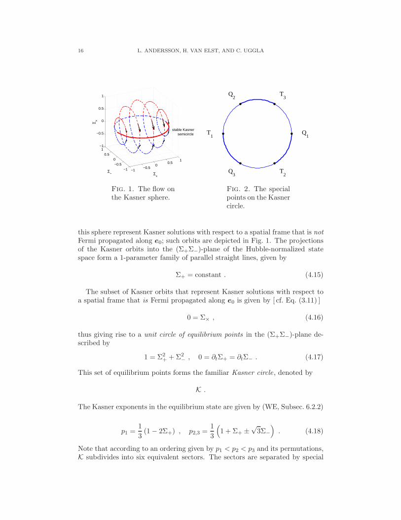
These equations define a flow on the unit sphere in Σ-space, with coordinates(Σ+,Σ−,Σ×), which we refer to as the Kasner sphere. The Kasner orbits on


−1−0.5

00.5

1

−1−0.50

0.51

−1

−0.5

0

0.5

1

← stable Kasner semicircle

Σ+

Σ−

Σ ×

Fig. 1. The flow onthe Kasner sphere.

T1

T2

T3

Q1

Q2

Q3

Fig. 2. The specialpoints on the Kasnercircle.

this sphere represent Kasner solutions with respect to a spatial frame that is notFermi propagated along e0; such orbits are depicted in Fig. 1. The projectionsof the Kasner orbits into the (Σ+Σ−)-plane of the Hubble-normalized statespace form a 1-parameter family of parallel straight lines, given by

Σ+ = constant . (4.15)

The subset of Kasner orbits that represent Kasner solutions with respect toa spatial frame that is Fermi propagated along e0 is given by [ cf. Eq. (3.11) ]

0 = Σ× , (4.16)

thus giving rise to a unit circle of equilibrium points in the (Σ+Σ−)-plane de-scribed by

1 = Σ2+ +Σ2

−, 0 = ∂tΣ+ = ∂tΣ− . (4.17)

This set of equilibrium points forms the familiar Kasner circle, denoted by

K .

The Kasner exponents in the equilibrium state are given by (WE, Subsec. 6.2.2)

p1 =1

3(1− 2Σ+) , p2,3 =

1

3

(

1 + Σ+ ±√3Σ−

)

. (4.18)

Note that according to an ordering given by p1 < p2 < p3 and its permutations,K subdivides into six equivalent sectors. The sectors are separated by special


points for which the variable pair (Σ+,Σ−) takes the fixed values

Q1 : (1, 0) , T3 :

(

1

2,

√3

2

)

,

Q2 :

(

− 1

2,

√3

2

)

, T1 : (− 1, 0) ,

Q3 :

(

− 1

2,−

√3

2

)

, T2 :

(

1

2,−

√3

2

)

,

so that two of the Kasner exponents become equal. The points Qα correspondto Kasner solutions that are locally rotationally symmetric, while the pointsTα correspond to Taub’s representation of the Minkowski solution (see WE,Subsec. 6.2.2, for further details).

5. Asymptotic dynamics towards the singularity

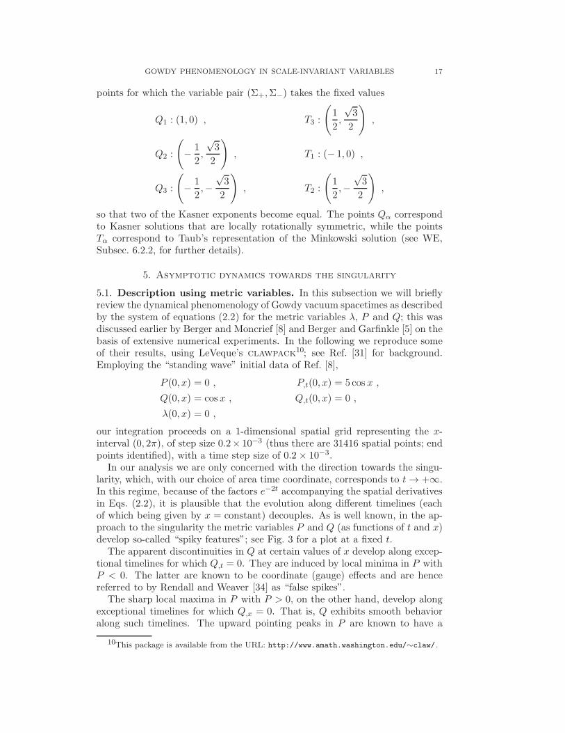
5.1. Description using metric variables. In this subsection we will brieflyreview the dynamical phenomenology of Gowdy vacuum spacetimes as describedby the system of equations (2.2) for the metric variables λ, P and Q; this wasdiscussed earlier by Berger and Moncrief [8] and Berger and Garfinkle [5] on thebasis of extensive numerical experiments. In the following we reproduce someof their results, using LeVeque’s clawpack10; see Ref. [31] for background.Employing the “standing wave” initial data of Ref. [8],

P (0, x) = 0 , P,t(0, x) = 5 cos x ,

Q(0, x) = cos x , Q,t(0, x) = 0 ,

λ(0, x) = 0 ,

our integration proceeds on a 1-dimensional spatial grid representing the x-interval (0, 2π), of step size 0.2× 10−3 (thus there are 31416 spatial points; endpoints identified), with a time step size of 0.2 × 10−3.

In our analysis we are only concerned with the direction towards the singu-larity, which, with our choice of area time coordinate, corresponds to t → +∞.In this regime, because of the factors e−2t accompanying the spatial derivativesin Eqs. (2.2), it is plausible that the evolution along different timelines (eachof which being given by x = constant) decouples. As is well known, in the ap-proach to the singularity the metric variables P and Q (as functions of t and x)develop so-called “spiky features”; see Fig. 3 for a plot at a fixed t.

The apparent discontinuities in Q at certain values of x develop along excep-tional timelines for which Q,t = 0. They are induced by local minima in P withP < 0. The latter are known to be coordinate (gauge) effects and are hencereferred to by Rendall and Weaver [34] as “false spikes”.

The sharp local maxima in P with P > 0, on the other hand, develop alongexceptional timelines for which Q,x = 0. That is, Q exhibits smooth behavioralong such timelines. The upward pointing peaks in P are known to have a

10This package is available from the URL: http://www.amath.washington.edu/∼claw/.

http://www.amath.washington.edu/~claw/

http://www.amath.washington.edu/~claw/


1 2 3 4 5 6

0

20

40

60

80

100

← "false spike" in Q

← Q

P →

Fig. 3. P and Q at t = 40.

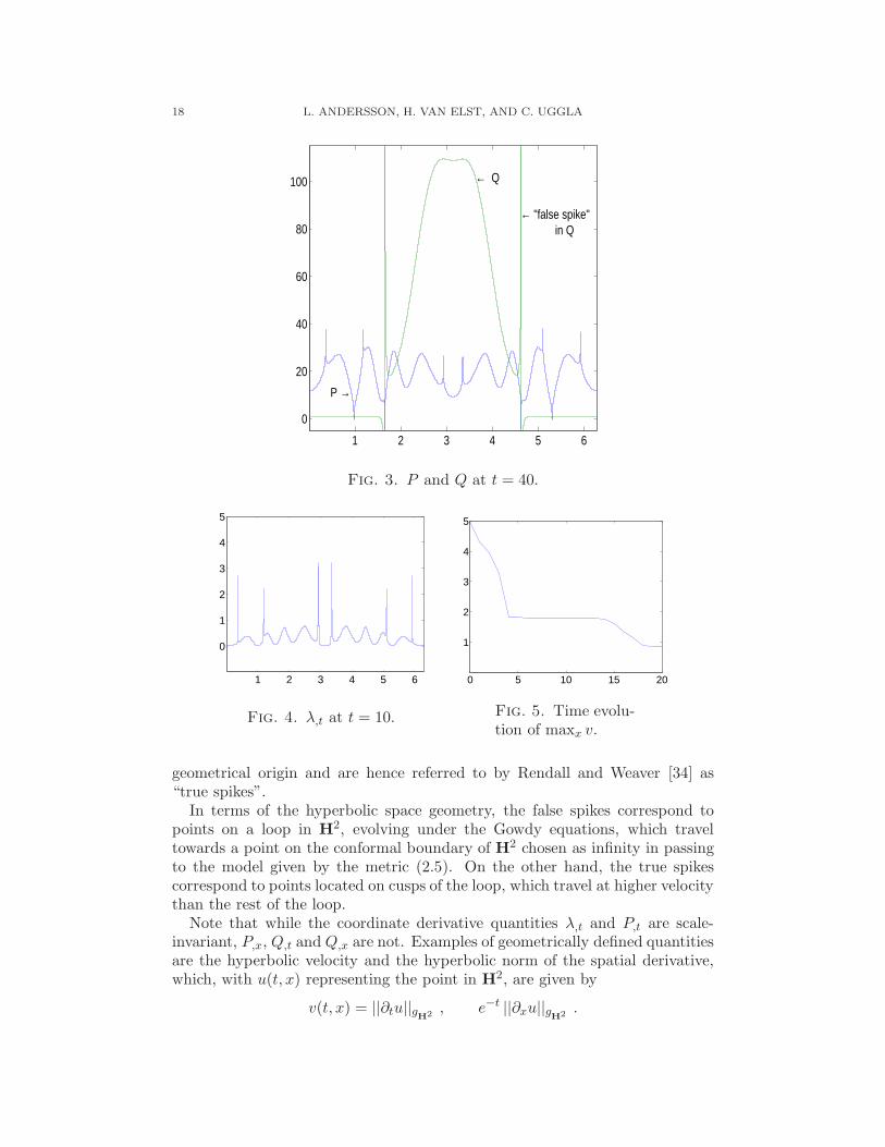
1 2 3 4 5 6

0

1

2

3

4

5

Fig. 4. λ,t at t = 10.

0 5 10 15 20

1

2

3

4

5

Fig. 5. Time evolu-tion of maxx v.

geometrical origin and are hence referred to by Rendall and Weaver [34] as“true spikes”.

In terms of the hyperbolic space geometry, the false spikes correspond topoints on a loop in H2, evolving under the Gowdy equations, which traveltowards a point on the conformal boundary of H2 chosen as infinity in passingto the model given by the metric (2.5). On the other hand, the true spikescorrespond to points located on cusps of the loop, which travel at higher velocitythan the rest of the loop.

Note that while the coordinate derivative quantities λ,t and P,t are scale-invariant, P,x, Q,t and Q,x are not. Examples of geometrically defined quantitiesare the hyperbolic velocity and the hyperbolic norm of the spatial derivative,which, with u(t, x) representing the point in H2, are given by

v(t, x) = ||∂tu||gH2

, e−t ||∂xu||gH2

.


Since we are using a logarithmic time coordinate, these two quantities are scale-invariant by construction. One is inexorably led to consider the scale-invariantoperators ∂t and e−t ∂x. In terms of the dimensional time coordinate τ = ℓ0e

−t,these operators are − τ ∂τ and τ ∂x, respectively.

The “energy density”, λ,t, depicted at a fixed t in Fig. 4, decreases moreslowly at spike points. Since we are not using an adaptive solver, we are notable to numerically resolve the behavior of λ,t at spike points. With u(t, x)representing the point in H2, however, we have from the Gauß constraint (2.3a)

λ,t(t, x) = v2(t, x) + e−2t ||∂xu||2gH2

,

where the second term is expected to tend to zero pointwise. Therefore, weexpect that λ,t asymptotically tends to a nonzero limit pointwise, given by theasymptotic hyperbolic velocity which we define as

v(x) := limt→+∞

v(t, x) , (5.1)

where the limit exists. As argued by Berger and Moncrief [8] and Berger andGarfinkle [5], the dynamics force the hyperbolic velocity to values v ≤ 1 at latetimes, except along timelines where spikes form; see Fig. 5. The reason maxx vappears to be less than 1 at late times in Fig. 5 is that the spikes have becomeso narrow that they are not resolved numerically.

Rendall and Weaver [34] have shown how to construct Gowdy solutions withboth false and true spikes from smooth solutions by a hyperbolic inversionfollowed by an Ernst transformation. In particular, they show that along thoseexceptional timelines, x = xtSpike, where (in numerical simulations) true spikesform as t → +∞, the asymptotic hyperbolic velocity satisfies v(xtSpike) = 1+s,with s ∈ (0, 1). On the other hand, along nearby, typical, timelines the limitingvalue is v = 1 − s. The speed at which v approaches v = 1 − s along thelatter timelines decreases rapidly as x approaches xtSpike. For the exceptionaltimelines, x = xfSpike, where (in numerical simulations) false spikes form ast → +∞, the asymptotic hyperbolic velocity satisfies v(xfSpike) = s, again withs ∈ (0, 1). Nearby, typical, timelines have limiting velocities v close to s. Theregimes 1 < v(xtSpike) < 2 and 0 < v(xfSpike) < 1 are referred to by Garfinkleand Weaver [21] as the regimes of “low velocity spikes”.

The true spikes with v(xtSpike) ∈ (1, 2) correspond, as has been known for along time, to simple zeros of Q,x. Higher velocity spikes were also constructedby Rendall and Weaver. However, these correspond to higher order zeros ofQ,x, and are therefore nongeneric.

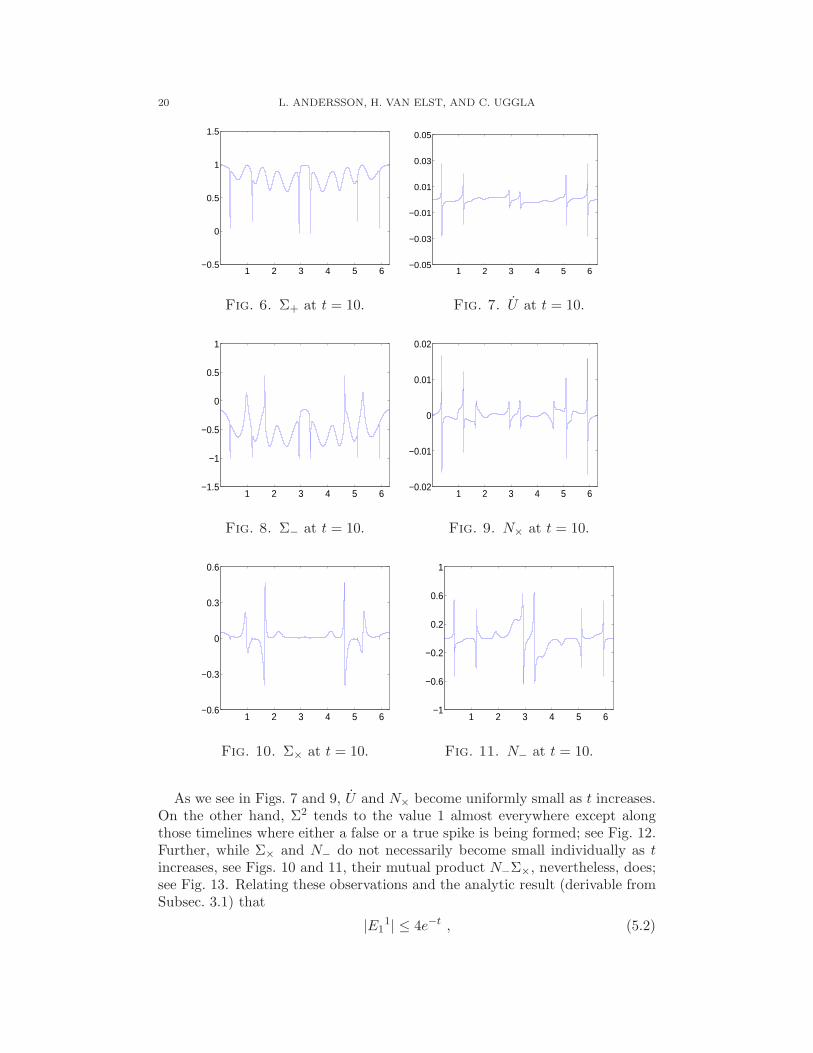
5.2. Description using Hubble-normalized variables. Here we first de-scribe the behavior of the Hubble-normalized variables Σ+, Σ−, N×, Σ×, N−

and U , when expressed in terms of the metric variables λ, P and Q and theircoordinate derivatives as in Eqs. (3.18), under the numerical integration of theGowdy equations (2.2)–(2.3). We use the same “standing wave” initial data asin Subsec. 5.1. The spatial variation of the values of the Hubble-normalizedvariables at a fixed t is depicted in Figs. 6–11. Note, in particular, the scalesalong the vertical axes in these figures.


1 2 3 4 5 6−0.5

0

0.5

1

1.5

Fig. 6. Σ+ at t = 10.

1 2 3 4 5 6−0.05

−0.03

−0.01

0.01

0.03

0.05

Fig. 7. U at t = 10.

1 2 3 4 5 6−1.5

−1

−0.5

0

0.5

1

Fig. 8. Σ− at t = 10.

1 2 3 4 5 6−0.02

−0.01

0

0.01

0.02

Fig. 9. N× at t = 10.

1 2 3 4 5 6−0.6

−0.3

0

0.3

0.6

Fig. 10. Σ× at t = 10.

1 2 3 4 5 6−1

−0.6

−0.2

0.2

0.6

1

Fig. 11. N− at t = 10.

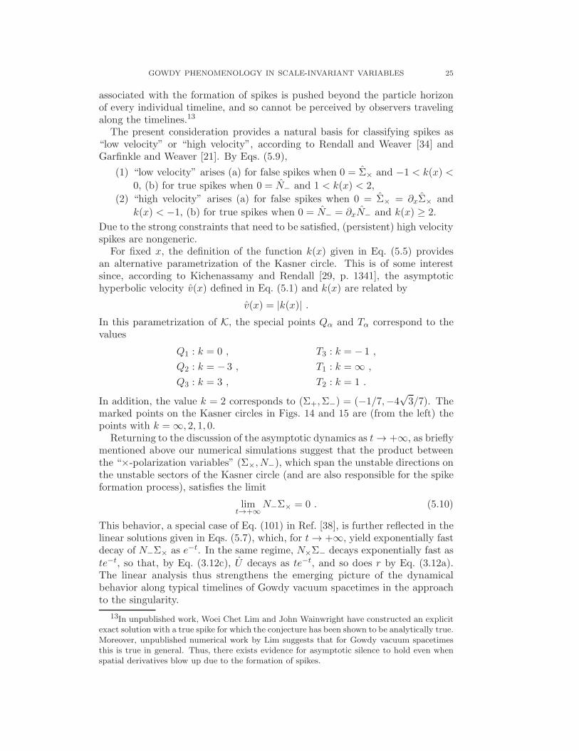
As we see in Figs. 7 and 9, U and N× become uniformly small as t increases.On the other hand, Σ2 tends to the value 1 almost everywhere except alongthose timelines where either a false or a true spike is being formed; see Fig. 12.Further, while Σ× and N− do not necessarily become small individually as tincreases, see Figs. 10 and 11, their mutual product N−Σ×, nevertheless, does;see Fig. 13. Relating these observations and the analytic result (derivable fromSubsec. 3.1) that

|E11| ≤ 4e−t , (5.2)


1 2 3 4 5 60.4

0.6

0.8

1

1.2

Fig. 12. Σ2 at t = 10.

1 2 3 4 5 6−0.01

−0.005

0

0.005

0.01

Fig. 13. N−Σ× att = 10.

so E11 → 0 uniformly as t → +∞, to the system of equations (3.12)–(3.14)

suggests that, in the approach to the singularity, for Gowdy vacuum space-times the ultra-strong spacetime curvature phenomenon of asymptotic silence,described in Refs. [20, §5.3] and [38, §4.1], sets in. Asymptotic silence refersto the collapse of the local null cones onto the timelines as t → +∞, withthe physical consequence that the propagation of gravitational waves betweenneighboring timelines is gradually frozen in. Based on these considerations, it isnatural to expect that near the singularity the spatial derivatives of the Hubble-normalized connection variables become dynamically irrelevant, and that thus,in a neighborhood of the silent boundary of the Hubble-normalized state space,the dynamics of Gowdy vacuum spacetimes is well approximated by the dy-namics on the silent boundary. More precisely, it is well approximated by thesystem of equations (3.12b), (3.12c), (4.2), (4.3) and (4.1a), but note that theHubble-normalized variables are now x-dependent. This aspect of the asymp-totic dynamics may also be viewed as a consequence of the friction term τ−1 ∂τin Eq. (2.6). In Figs. 14 and 15 we show the projections into the (Σ+Σ−)-planeof the Hubble-normalized state space of orbits for (i) the evolution system onthe silent boundary, Eqs. (4.2), and (ii) a typical timeline of the full Gowdyevolution equations (3.13). It is apparent that qualitative features of the full

Gowdy evolution system along an individual timeline are correctly reproduced

by the evolution system on the silent boundary.

To gain further insight into the dynamics towards the singularity, we will nowinvestigate the local stability of the Kasner circle K on the silent boundary ofthe Hubble-normalized state space for Gowdy vacuum spacetimes, thus probingthe closest parts of the interior of the state space.

5.2.1. Linearized dynamics at the Kasner circle on the silent boundary. Werecall that on the silent boundary the Hubble-normalized variables are x-depen-dent. Consequently, the Kasner circle K on the silent boundary is representedby the conditions

0 = E11 = Σ× = N× = N− = U = r , Σ+ = Σ+ , Σ− = Σ− , (5.3a)

1 = Σ2+ + Σ2

−, q = 2 , (5.3b)


−1 0 1 2−2

−1

0

1

2

Σ+

Σ −

Fig. 14. Projectioninto the (Σ+Σ−)-plane of an orbit de-termined by the SBsystem (4.2).

−1 0 1 2−2

−1

0

1

2

Σ+

Σ −

Fig. 15. Projectioninto the (Σ+Σ−)-plane of a Gowdy or-bit along the typicaltimeline x = 2.7.

where we introduce the convention that “hatted” variables are functions of thespatial coordinate x only. Thus, linearizing the Hubble-normalized Gowdy evo-lution equations (3.13) on the silent boundary at an equilibrium point (Σ+, Σ−)of K yields (with C = − 1

2)

∂tE11 = −E1

1 , (5.4a)

∂tδΣ+ = − 2 (Σ+ δΣ+ + Σ− δΣ−) , (5.4b)

∂tδΣ− = − 2Σ−

(1 + Σ+)(Σ+ δΣ+ + Σ− δΣ−) , (5.4c)

∂tN× = −N× +1

2

∂xΣ−

(1 + Σ+)E1

1 , (5.4d)

∂tΣ× =

√3Σ−

(1 + Σ+)Σ× , (5.4e)

∂tN− = −[

1 +

√3Σ−

(1 + Σ+)

]

N− ; (5.4f)

here δΣ+ and δΣ− denote the deviations in Σ+ and Σ− from their equilibrium

values Σ+ and Σ− on K. Let us define an x-dependent function

k(x) := −√3Σ−(x)

1 + Σ+(x), (5.5)


corresponding to a particular function used in Refs. [29] and [34]. Then, inte-grating Eqs. (5.4) with respect to t, we find for E1

1, δΣ+, δΣ− and N×

E11 = O(e−t) , (5.6a)

δΣ+ = O(e−t) , (5.6b)

δΣ− = O(e−t) , (5.6c)

N× = N× e−t +O(te−t) . (5.6d)

That is, as t → +∞, the solutions for E11, δΣ+ and δΣ− decay exponentially

fast as e−t, while N× decays exponentially fast as te−t, independent of the

values of (Σ+, Σ−) [ and so k(x) ] along an individual timeline. Consequently,these variables are stable on K. The solutions for the variable pair (Σ×, N−)associated with the “×-polarization state”, on the other hand, are given by

Σ× = Σ× e−k(x)t , (5.7a)

N− = N− e−[1−k(x)]t , (5.7b)

(see also Eqs. (140) and (141) in Ref. [20]).11 Thus,

(1) Σ× is an unstable variable on K as t → +∞ whenever k(x) < 0; this

happens along timelines for which the values of (Σ+, Σ−) define a point

on the upper semicircle of K (unless, of course, 0 = Σ× along such atimeline), and

(2) N− is an unstable variable on K as t → +∞ whenever k(x) > 1; this

happens along timelines for which the values of (Σ+, Σ−) define a pointeither on the arc(T1Q3) ⊂ K or on the arc(Q3T2) ⊂ K (unless, of course,

0 = N− along such a timeline).

This implies that in the approach to the singularity, the Kasner equilibriumset K in the Hubble-normalized state space of every individual timeline has a1-dimensional unstable manifold , except when the values of (Σ+, Σ−) coincidewith those of the special points Qα and Tα, or correspond to points on thearc(T2Q1) ⊂ K which is stable.12

Close to the singularity (and so to the silent boundary of the state space),

it follows that along those timelines where (Σ+, Σ−) take values in the Σ×-unstable sectors of K, a frame transition orbit of Bianchi Type–I according toEq. (4.15) to the Σ×-stable part of K is induced (corresponding to a rotationof the spatial frame by π/2 about the e1-axis). Notice that timelines along

which 0 = Σ× do not participate in these frame transitions and so are “leftbehind” by the asymptotic dynamics. This provides a simple mechanism forthe gradual formation of false spikes on T3. As, by Eq. (3.11), Σ× quantifiesthe Hubble-normalized angular velocity at which e2 and e3 rotate about e1(the latter being a spatial frame gauge variable), false spikes clearly are a gaugeeffect.

11Altogether, the linear solutions contain four arbitrary 2π-periodic real-valued functions

of x, namely k, N×, Σ× and N−.12For the polarized invariant set, on the other hand, here included as the special case

0 = Σ× = N−, the entire Kasner equilibrium set K is stable.


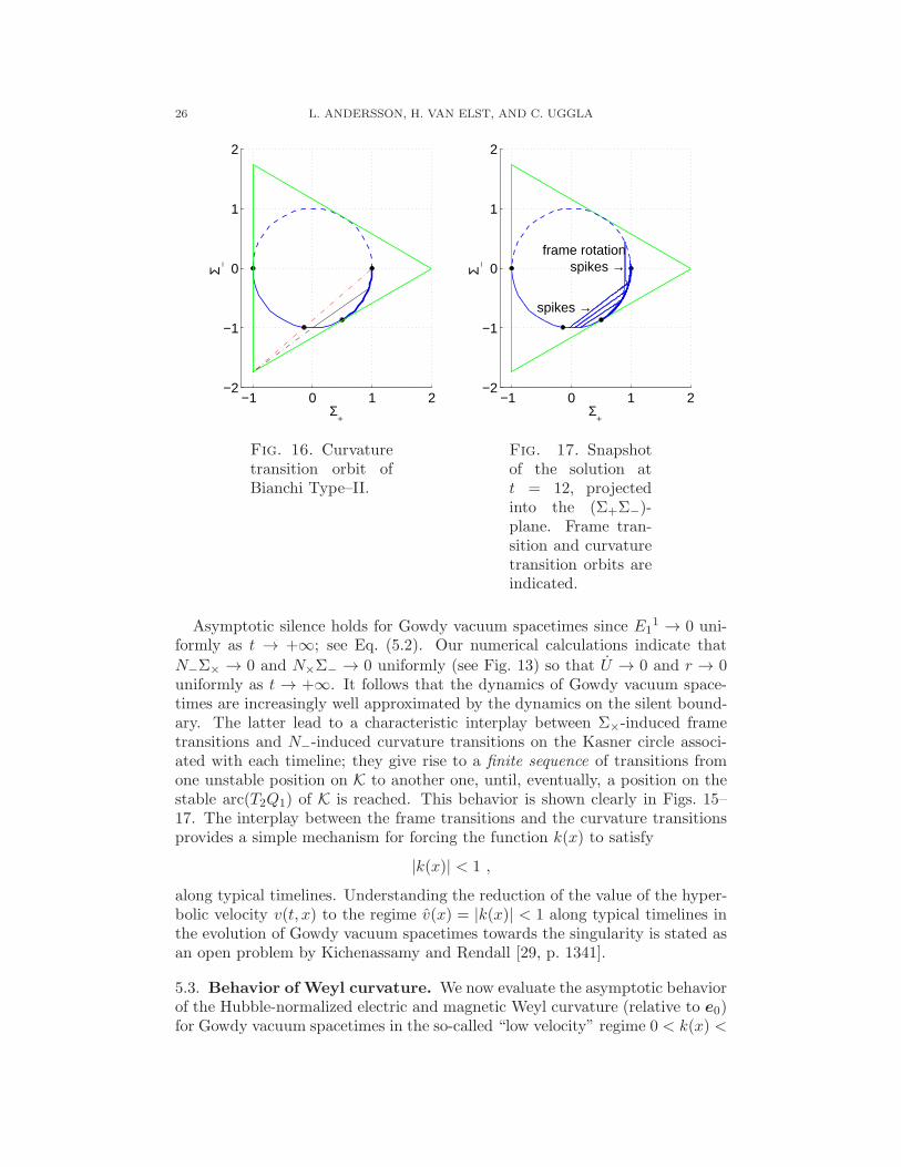
On the other hand, along those timelines where (Σ+, Σ−) take values inthe N−-unstable sectors of K, a curvature transition orbit of Bianchi Type–IIaccording to Eq. (4.11) to the N−-stable part of K is induced; this is shown in

Fig. 16. Notice that timelines along which 0 = N− do not participate in thesecurvature transitions and so are “left behind” by the asymptotic dynamics.This provides a simple mechanism for the gradual formation of true spikeson T3. As N− presently relates to the intrinsic curvature of T3, true spikes area geometrical effect.

It was pointed out in Ref. [38, §4.1] that it is natural to expect from theconsideration of asymptotic silence that

limt→+∞

E11 ∂xY = 0 (5.8)

is satisfied along typical timelines; in our case Y = (Σ+,Σ−, N×,Σ×, N−)T .

This limit is certainly attained for each of Σ+, Σ− and N× when we use thelinear solutions of Eqs. (5.6) for these variables which are valid in a neighbor-hood of K on the silent boundary. For the “×-polarization variables” (Σ×, N−)an analogous substitution from Eqs. (5.7) leads to

E11 ∂xΣ× ∝

(

∂xΣ× − t Σ× ∂xk(x))

e−[1+k(x)]t , (5.9a)

E11 ∂xN− ∝

(

∂xN− + t N− ∂xk(x))

e−[2−k(x)]t . (5.9b)

Here a number of cases arise when we consider the behavior of these spatialderivative expressions in the limit t → +∞. Firstly, both decay exponentiallyfast along those timelines for which the dynamics has entered the regime 0 ≤k(x) < 1. As discussed in some detail below, this happens asymptotically along

typical timelines. Secondly, along timelines where false spikes (0 = Σ×) form,both decay exponentially fast when the dynamics is confined to the regime−1 < k(x) < 0. Thirdly, along timelines where true spikes (0 = N−) form,both decay exponentially fast when the dynamics is confined to the regime1 < k(x) < 2. Outside the regime −1 < k(x) < 2, one or the other of thespatial derivative expressions (5.9) may grow temporarily along timelines, untilone of the unstable modes (5.7) drives the dynamics towards a neighborhoodof a different sector of K. Also, outside the regime −1 < k(x) < 2, spikes ofhigher order may form along exceptional timelines, through choice of specialinitial conditions.

In recent numerical work, Garfinkle and Weaver [21] investigated spikes withk(x) initially outside the regime −1 < k(x) < 2 and reported that they generallydisappear in the process of evolution. It has been suggested by Lim [32] that so-called spike transition orbits could provide an explanation for this phenomenon.Unfortunately, no analytic approximations are available to date and furtherwork is needed. Nevertheless, numerical experiments so far indicate that thelimit (5.8) does hold for timelines with nonspecial initial conditions [32].

According to a conjecture by Uggla et al [38, §4.1], the exceptional dynamicalbehavior towards the singularity along those timelines where either false ortrue spikes form does not disturb the overall asymptotically silent nature of thedynamics, as in the (here) asymptotic limit t → +∞ any spatial inhomogeneity


associated with the formation of spikes is pushed beyond the particle horizonof every individual timeline, and so cannot be perceived by observers travelingalong the timelines.13

The present consideration provides a natural basis for classifying spikes as“low velocity” or “high velocity”, according to Rendall and Weaver [34] andGarfinkle and Weaver [21]. By Eqs. (5.9),

(1) “low velocity” arises (a) for false spikes when 0 = Σ× and −1 < k(x) <

0, (b) for true spikes when 0 = N− and 1 < k(x) < 2,

(2) “high velocity” arises (a) for false spikes when 0 = Σ× = ∂xΣ× and

k(x) < −1, (b) for true spikes when 0 = N− = ∂xN− and k(x) ≥ 2.

Due to the strong constraints that need to be satisfied, (persistent) high velocityspikes are nongeneric.

For fixed x, the definition of the function k(x) given in Eq. (5.5) providesan alternative parametrization of the Kasner circle. This is of some interestsince, according to Kichenassamy and Rendall [29, p. 1341], the asymptotichyperbolic velocity v(x) defined in Eq. (5.1) and k(x) are related by

v(x) = |k(x)| .In this parametrization of K, the special points Qα and Tα correspond to thevalues

Q1 : k = 0 , T3 : k = − 1 ,

Q2 : k = − 3 , T1 : k = ∞ ,

Q3 : k = 3 , T2 : k = 1 .

In addition, the value k = 2 corresponds to (Σ+,Σ−) = (−1/7,−4√3/7). The

marked points on the Kasner circles in Figs. 14 and 15 are (from the left) thepoints with k = ∞, 2, 1, 0.

Returning to the discussion of the asymptotic dynamics as t → +∞, as brieflymentioned above our numerical simulations suggest that the product betweenthe “×-polarization variables” (Σ×, N−), which span the unstable directions onthe unstable sectors of the Kasner circle (and are also responsible for the spikeformation process), satisfies the limit

limt→+∞

N−Σ× = 0 . (5.10)

This behavior, a special case of Eq. (101) in Ref. [38], is further reflected in thelinear solutions given in Eqs. (5.7), which, for t → +∞, yield exponentially fastdecay of N−Σ× as e−t. In the same regime, N×Σ− decays exponentially fast aste−t, so that, by Eq. (3.12c), U decays as te−t, and so does r by Eq. (3.12a).The linear analysis thus strengthens the emerging picture of the dynamicalbehavior along typical timelines of Gowdy vacuum spacetimes in the approachto the singularity.

13In unpublished work, Woei Chet Lim and John Wainwright have constructed an explicitexact solution with a true spike for which the conjecture has been shown to be analytically true.Moreover, unpublished numerical work by Lim suggests that for Gowdy vacuum spacetimesthis is true in general. Thus, there exists evidence for asymptotic silence to hold even whenspatial derivatives blow up due to the formation of spikes.


−1 0 1 2−2

−1

0

1

2

Σ+

Σ −

Fig. 16. Curvaturetransition orbit ofBianchi Type–II.

−1 0 1 2−2

−1

0

1

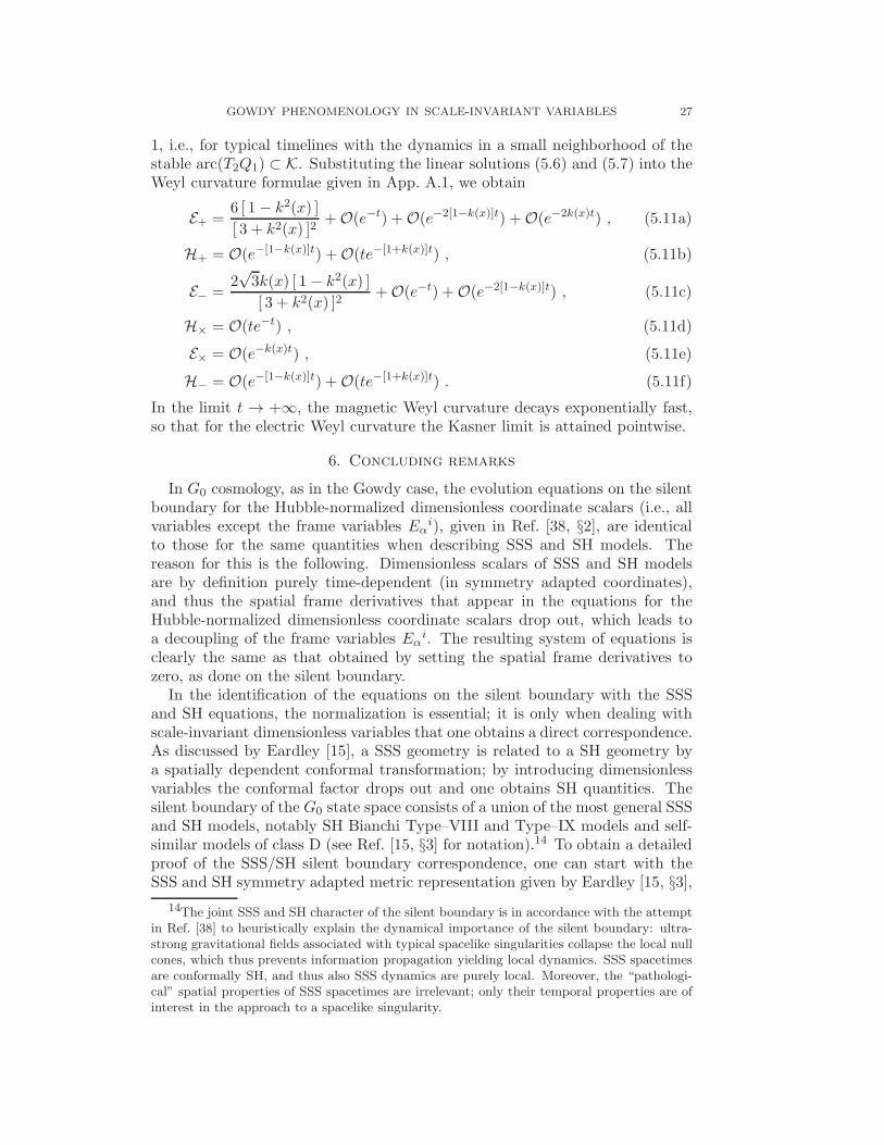
2

frame rotation spikes →

spikes →

Σ+

Σ −

Fig. 17. Snapshotof the solution att = 12, projectedinto the (Σ+Σ−)-plane. Frame tran-sition and curvaturetransition orbits areindicated.

Asymptotic silence holds for Gowdy vacuum spacetimes since E11 → 0 uni-

formly as t → +∞; see Eq. (5.2). Our numerical calculations indicate that

N−Σ× → 0 and N×Σ− → 0 uniformly (see Fig. 13) so that U → 0 and r → 0uniformly as t → +∞. It follows that the dynamics of Gowdy vacuum space-times are increasingly well approximated by the dynamics on the silent bound-ary. The latter lead to a characteristic interplay between Σ×-induced frametransitions and N−-induced curvature transitions on the Kasner circle associ-ated with each timeline; they give rise to a finite sequence of transitions fromone unstable position on K to another one, until, eventually, a position on thestable arc(T2Q1) of K is reached. This behavior is shown clearly in Figs. 15–17. The interplay between the frame transitions and the curvature transitionsprovides a simple mechanism for forcing the function k(x) to satisfy

|k(x)| < 1 ,

along typical timelines. Understanding the reduction of the value of the hyper-bolic velocity v(t, x) to the regime v(x) = |k(x)| < 1 along typical timelines inthe evolution of Gowdy vacuum spacetimes towards the singularity is stated asan open problem by Kichenassamy and Rendall [29, p. 1341].

5.3. Behavior of Weyl curvature. We now evaluate the asymptotic behaviorof the Hubble-normalized electric and magnetic Weyl curvature (relative to e0)for Gowdy vacuum spacetimes in the so-called “low velocity” regime 0 < k(x) <


1, i.e., for typical timelines with the dynamics in a small neighborhood of thestable arc(T2Q1) ⊂ K. Substituting the linear solutions (5.6) and (5.7) into theWeyl curvature formulae given in App. A.1, we obtain

E+ =6 [ 1 − k2(x) ]

[ 3 + k2(x) ]2+O(e−t) +O(e−2[1−k(x)]t) +O(e−2k(x)t) , (5.11a)

H+ = O(e−[1−k(x)]t) +O(te−[1+k(x)]t) , (5.11b)

E− =2√3k(x) [ 1 − k2(x) ]

[ 3 + k2(x) ]2+O(e−t) +O(e−2[1−k(x)]t) , (5.11c)

H× = O(te−t) , (5.11d)

E× = O(e−k(x)t) , (5.11e)

H− = O(e−[1−k(x)]t) +O(te−[1+k(x)]t) . (5.11f)

In the limit t → +∞, the magnetic Weyl curvature decays exponentially fast,so that for the electric Weyl curvature the Kasner limit is attained pointwise.

6. Concluding remarks

In G0 cosmology, as in the Gowdy case, the evolution equations on the silentboundary for the Hubble-normalized dimensionless coordinate scalars (i.e., allvariables except the frame variables Eα

i), given in Ref. [38, §2], are identicalto those for the same quantities when describing SSS and SH models. Thereason for this is the following. Dimensionless scalars of SSS and SH modelsare by definition purely time-dependent (in symmetry adapted coordinates),and thus the spatial frame derivatives that appear in the equations for theHubble-normalized dimensionless coordinate scalars drop out, which leads toa decoupling of the frame variables Eα

i. The resulting system of equations isclearly the same as that obtained by setting the spatial frame derivatives tozero, as done on the silent boundary.

In the identification of the equations on the silent boundary with the SSSand SH equations, the normalization is essential; it is only when dealing withscale-invariant dimensionless variables that one obtains a direct correspondence.As discussed by Eardley [15], a SSS geometry is related to a SH geometry bya spatially dependent conformal transformation; by introducing dimensionlessvariables the conformal factor drops out and one obtains SH quantities. Thesilent boundary of the G0 state space consists of a union of the most general SSSand SH models, notably SH Bianchi Type–VIII and Type–IX models and self-similar models of class D (see Ref. [15, §3] for notation).14 To obtain a detailedproof of the SSS/SH silent boundary correspondence, one can start with theSSS and SH symmetry adapted metric representation given by Eardley [15, §3],

14The joint SSS and SH character of the silent boundary is in accordance with the attemptin Ref. [38] to heuristically explain the dynamical importance of the silent boundary: ultra-strong gravitational fields associated with typical spacelike singularities collapse the local nullcones, which thus prevents information propagation yielding local dynamics. SSS spacetimesare conformally SH, and thus also SSS dynamics are purely local. Moreover, the “pathologi-cal” spatial properties of SSS spacetimes are irrelevant; only their temporal properties are ofinterest in the approach to a spacelike singularity.


and then derive the correspondence through a direct comparison between theSSS/SH equations and those on the silent boundary.

Gowdy vacuum spacetimes form an invariant set of the general G0 statespace. The intersection of this invariant set with the SSS and SH subsets inturn yields an invariant subset which is described by the equations on the silentboundary of the Gowdy state space.

6.1. AVTD and BKL from the point of view of the silent boundary.

Discussions of AVTD behavior near spacetime singularities and of the BKLconjecture on oscillatory behavior of vacuum dominated singularities have of-ten been associated with claims that the asymptotic dynamical behavior inthe direction of the singularity of spatially inhomogenous spacetimes is locallylike that of SH models. Indeed, BKL take as a starting point for their anal-ysis explicit SH solutions. They replace the integration constants by spatiallydependent functions and perform a perturbation analysis in the asymptoticregime around the resulting ansatz. The dynamical systems approach offerssome justification for this procedure.15

Due to the SSS/SH silent boundary correspondence, the reduced system ofequations on the silent boundary leads to the same solutions for the Hubble-normalized coordinate scalars in both cases. However, in contrast to the trueSSS/SH cases, the constants of integration become spatially dependent func-tions on the silent boundary. Then, in the true SSS/SH cases, the metric is ob-tained in a subsequent step, by integrating the decoupled system of equationsfor the frame variables Eα

i. However, the silent boundary (where 0 = Eαi)

is unphysical, since it corresponds to a degenerate metric. In order to obtainan expression for the metric which is valid in the asymptotic regime, one isforced to go into the physical interior part of the state space where the Eα

i arenonzero. By perturbing around 0 = Eα

i, starting from a seed solution to thereduced system of equations on the silent boundary, approximate solutions tothe full system can be constructed. To lowest order, the asymptotic approxi-mation so obtained is identical to the corresponding true SSS/SH solution, butwith integration constants replaced by spatially dependent functions which inturn are restricted by the Codacci constraint.

In terms of the discussion in this paper, the AVTD leading order solutionfor Gowdy vacuum spacetimes is produced by the above procedure using a seedsolution taking values in the Kasner subset on the silent boundary (note thatVTD is associated with the entire silent Kasner subset, while AVTD is associ-ated only with the stable part(s) of the Kasner circle). Indeed, the linearizationat the stable arc of the Kasner circle yields the starting point for the analysisof Kichenassamy and Rendall [29]. Similarly, BKL in their analysis considerseed data in the Taub subset (vacuum Bianchi Type–II) on the silent bound-ary, in addition to the Kasner subset. Thus, the AVTD and BKL analysis has

15An alternative point of view on the oscillatory approach to the singularity is providedby the method of consistent potentials (see Ref. [7] for a discussion of the T 2-symmetriccase). Further, Thibault Damour, Marc Henneaux and collaborators have recently developeda picture of the asymptotic behavior of stringy gravity in D = 10 spacetime dimensions, whichleads to consideration of hyperbolic billiards (see Refs. [13] and [14], and references therein).


considered only part of the past attractor conjectured in Ref. [38], while on thecontrary, the results in the present paper indicate that it is essential to considerthe entire silent boundary in order to understand the approach towards thesingularity.

6.2. Gowdy case. We conclude by discussing the picture that emerges in theGowdy case. In view of the non-oscillatory nature of the system of equationson the silent boundary, we expect Gowdy vacuum spacetimes to have a non-oscillatory singularity in the sense that limt→+∞X(t, x) = X(x) exists, and

that X takes values only on the Kasner circle K on the silent boundary. More-over, the local stability of the arc(T2Q1) ⊂ K suggests that it is a local attractor,i.e.,

A = arc(T2Q1) ⊂ K = A−

Gowdy .

This was indeed proved by Ringstrom [36, 37] and Chae and Chrusciel [9]: ifX(t, x) is sufficiently close to A, in a suitable sense, then limt→+∞X(t, x) =

X(x), with X(x): S1 → A a continuous map, and the limit is in the uni-form topology. Chae and Chrusciel [9] have also proved that for any Gowdyvacuum spacetime with smooth initial data, there is an open and dense sub-set O ⊂ S1, such that for x ∈ O, limt→+∞X(t, x) = X(x), X(x) ∈ A, and

X is smooth at x. Furthermore, they showed that, for any closed F ⊂ S1

with empty interior, a solution could be constructed with (false) spikes on F .By applying Gowdy-to-Ernst transformations, these can presumably be turnedinto true spikes with high velocity. This shows that the detailed asymptoticbehavior of Gowdy vacuum spacetimes can be quite complicated. A very usefulfurther step in the mathematical analysis of Gowdy vacuum spacetimes wouldbe to prove that it is always the case that limt→+∞(Σ−N×)

2 + (Σ×N−)2 = 0.

A limit of this kind reflects that in the asymptotic regime the propagation ofgravitational waves (represented by the “+ -polarization variables” (Σ−, N×)and the “×-polarization variables” (Σ×, N−), respectively) becomes dynami-cally insignificant.

If one considers generic smooth initial data, the picture should simplify con-siderably. For example, since a generic smooth function has at most a finitenumber of zeros on a finite interval, and true spikes correspond to zeros ofQ,x, one expects that generic solutions have at most a finite number of truespikes. An analogous argument indicates that a generic solution has at most afinite number of (true or false) spikes. High velocity spikes are expected to benongeneric since they correspond to higher order zeros of Q,x. Therefore, oneexpects that a generic solution will have a finite number of true spikes, all withvelocity in the interval (1, 2).

Due to the existence of spikes for general Gowdy vacuum spacetimes, A can-

not be a global attractor. For a Gowdy solution with spikes,

limt→+∞

supx∈S1

d(X(t, x),K) 6= 0 ,

even though we expect that the pointwise limit is a map to K. This makesit clear that the notions of “asymptotic state” and “attractor” depend, in thespatially inhomogenous case, on the choice of topology.


The numerical work in this paper indicates that the variety

U = Σ−N× = Σ×N− = 0

is the uniform attractor for Gowdy vacuum spacetimes in the sense that

limt→+∞

supx∈S1

d(X(t, x),U) = 0 .

As seen from the discussion in Subsec. 5.2, the silent boundary dynamics on Uexplain the major evolutionary features along typical Gowdy timelines.

The state space framework for spatially inhomogeneous cosmology based onthe dynamical systems approach offers a common ground where many scatteredresults and conjectures may be collected and put into a broader context. Forexample, earlier claims and results as regards SH models can now be regardedas results determined by the structure of the silent boundary of the Hubble-normalized state space. This pertains, e.g., to work by BKL, conjectures andproofs in WE, and proofs by Ringstrom. The latter showed in Ref. [35] thatthe Bianchi Type–II variety is a past attractor for nontilted SH perfect fluidmodels of Bianchi Type–IX.16

Finally, earlier results, and the results in this paper, suggest that the silentboundary, perturbations thereof, and the formation of spikes, in a G2 as well asin a G0 context, are worthy areas of exploration, and are likely to offer excitinghunting grounds in the coming years.

Acknowledgments

We thank Woei Chet Lim, John Wainwright, and Piotr Chrusciel for helpfulcomments. Further, we are grateful to Mattias Sandberg for his work duringthe early stages of this project.

Appendix A. Hubble-normalized Weyl curvature

A.1. Variables. The Hubble-normalized electric and magnetic Weyl curva-tures (relative to e0) for Gowdy vacuum spacetimes can be easily obtained byspecializing the relations given in Ref. [18]. The “+”, “−” and “×” variables

16This attractor organizes the past asymptotic dynamics and provides an explanation forthe Kasner-billiard-like behavior of nontilted SH models of Bianchi Type–IX in the approachto the singularity. The same variety is expected to be the past attractor for nontilted SHmodels of Bianchi Type–VIII. A candidate attractor variety has been identified for nontiltedSH perfect fluid models of Bianchi Type–VI∗

−1/9 by Hewitt et al [25]. This is the only nontilted

SH model in class B that exhibits oscillatory dynamical behavior into the past.


are defined analogous to the shear rate variables in Eqs. (2.13).

E+ =2

3(N2

×+N2

−) +

1

3(1 + Σ+)Σ+ − 1

3(Σ2

−+Σ2

×) , (A.1a)

H+ = −N−Σ− −N×Σ× , (A.1b)

E− =1

3(E1

1 ∂x − r)N× +2√3N2

−+

1

3(1− 2Σ+)Σ− , (A.1c)

H× =1

3(E1

1 ∂x − r)Σ− − 2√3N−Σ× −N×Σ+ , (A.1d)

E× = − 1

3(E1

1 ∂x − r)N− +2√3N×N− +

1

3(1− 2Σ+)Σ× , (A.1e)

H− = − 1

3(E1

1 ∂x − r)Σ× − 2√3N−Σ− −N−Σ+ . (A.1f)

A.2. Spatial scalars.

EαβEαβ = 6(E2+ + E2

−+ E2

×) , (A.2a)

HαβHαβ = 6(H2+ +H2

−+H2

×) , (A.2b)

EαβHαβ = 6(E+H+ + E−H− + E×H×) , (A.2c)

EαβEβγEγα = − 6E+ (E2+ − 3E2

−− 3E2

×) , (A.2d)

HαβHβ

γHγα = − 6H+ (H2

+ − 3H2−− 3H2

×) , (A.2e)

EαβHβγHγ

α = − 6 [ E+ (H2+ −H2

−−H2

×)− 2E−H+H− − 2E×H+H× ] ,

(A.2f)

HαβEβγEγα = − 6 [H+ (E2

+ − E2−− E2

×)− 2H−E+E− − 2H×E+E× ] . (A.2g)

A.3. Spacetime scalars.

I1 = 8(EαβEαβ −HαβHαβ) , (A.3a)

I2 = − 16EαβHαβ , (A.3b)

I3 = − 16(EαβEβγEγα − 3EαβHβγHγ

α) , (A.3c)

I4 = 16(HαβHβ

γHγα − 3Hα

βEβγEγα) . (A.3d)

I1 is the Hubble-normalized Kretschmann scalar.

References

1. Guido Beck, Zur Theorie binarer Gravitationsfelder, Z. Phys. 33 (1925), 713–728.2. Vladimir A. Belinskiı, Isaac M. Khalatnikov, and Evgeny M. Lifshitz, Oscillatory approach

to a singular point in the relativistic cosmology, Adv. Phys. 19 (1970), 525–573.3. , A general solution of the Einstein equations with a time singularity, Adv. Phys.

31 (1982), 639–667.4. Beverly K. Berger, Approach to the singularity in spatially inhomogeneous cosmologies,

Differential equations and mathematical physics (Birmingham, AL, 1999), AMS/IP Stud.Adv. Math., vol. 16, Amer. Math. Soc., Providence, RI, 2000, pp. 27–40.

5. Beverly K. Berger and David Garfinkle, Phenomenology of the Gowdy universe on T 3×R,Phys. Rev. D 57 (1998), 4767–4777.


6. Beverly K. Berger, David Garfinkle, James Isenberg, Vincent Moncrief, and MarshaWeaver, The singularity in generic gravitational collapse is spacelike, local and oscilla-

tory, Modern Phys. Lett. A 13 (1998), no. 19, 1565–1573.7. Beverly K. Berger, James Isenberg, and Marsha Weaver, Oscillatory approach to the

singularity in vacuum spacetimes with T 2 isometry, Phys. Rev. D 64 (2001), no. 8, 084006–20.

8. Beverly K. Berger and Vincent Moncrief, Numerical investigation of cosmological singu-

larities, Phys. Rev. D 48 (1993), no. 10, 4676–4687.9. Myeongju Chae and Piotr T. Chrusciel, On the dynamics of Gowdy space-times, gr-

qc/0305029, 2003.10. Piotr T. Chrusciel, On space-times with U(1)×U(1) symmetric compact Cauchy surfaces,

Ann. Physics (N.Y.) 202 (1990), no. 1, 100–150.11. Piotr T. Chrusciel, James Isenberg, and Vincent Moncrief, Strong cosmic censorship in

polarised Gowdy spacetimes, Classical Quantum Gravity 7 (1990), no. 10, 1671–1680.12. C. Barry Collins, More qualitative cosmology, Commun. Math. Phys. 23 (1971), 137–158.13. Thibault Damour and Marc Henneaux, E10, BE10 and arithmetical chaos in superstring

cosmology, Phys. Rev. Lett. 86 (2001), no. 21, 4749–4752.14. Thibault Damour, Marc Henneaux, and Hermann Nicolai, Cosmological billiards, Classical

Quantum Gravity 20 (2003), no. 9, R145–R200.15. Douglas M. Eardley, Self-similar spacetimes: geometry and dynamics, Commun. Math.

Phys. 37 (1974), 287–309.16. Albert Einstein and Nathan Rosen, On gravitational waves, J. Franklin Inst. 223 (1937),

43–54.17. George F. R. Ellis and Malcolm A. H. MacCallum, A class of homogeneous cosmological

models, Commun. Math. Phys. 12 (1969), 108–141.18. Henk van Elst, Hubble-normalised orthonomal frame equations for perfect fluid cosmologies

in component form, URL: www.maths.qmul.ac.uk/~hve/research.html, 2002.19. Henk van Elst and Claes Uggla, General relativistic 1+3 orthonormal frame approach,

Classical Quantum Gravity 14 (1997), no. 9, 2673–2695.20. Henk van Elst, Claes Uggla, and John Wainwright, Dynamical systems approach to G2

cosmology, Classical Quantum Gravity 19 (2002), no. 1, 51–82.21. David Garfinkle and Marsha Weaver, High velocity spikes in Gowdy spacetimes, Phys.

Rev. D 67 (2003), no. 12, 124009–5.22. Robert H. Gowdy, Gravitational waves in closed universes, Phys. Rev. Lett. 27 (1971),

no. 12, 826–829.23. , Vacuum spacetimes and compact invariant hyperspaces: Topologies and boundary

conditions, Ann. Physics (N.Y.) 83 (1974), 203–241.24. Boro Grubisic and Vincent Moncrief, Asymptotic behavior of the T 3 × R Gowdy space-

times, Phys. Rev. D 47 (1993), no. 6, 2371–2382.25. Conrad G. Hewitt, Joshua T. Horwood, and John Wainwright, Asymptotic dynamics of the

exceptional Bianchi cosmologies, Classical Quantum Gravity 20 (2003), no. 9, 1743–1756.26. Conrad G. Hewitt and John Wainwright, Orthogonally transitive G2 cosmologies, Classical

Quantum Gravity 7 (1990), no. 12, 2295–2316.27. James Isenberg, Martin Jackson, and Vincent Moncrief, Evolution of the Bel–Robinson

energy in Gowdy T 3 ×R space-times, J. Math. Phys. 31 (1990), no. 2, 517–519.28. James Isenberg and Vincent Moncrief, Asymptotic behavior of the gravitational field and

the nature of singularities in Gowdy spacetimes, Ann. Physics (N.Y.) 199 (1990), no. 1,84–122.

29. Satyanad Kichenassamy and Alan D. Rendall, Analytic description of singularities in

Gowdy spacetimes, Classical Quantum Gravity 15 (1998), no. 5, 1339–1355.30. Andrew R. King and George F. R. Ellis, Tilted homogeneous cosmological models, Com-

mun. Math. Phys. 31 (1973), 209–242.31. Randall J. LeVeque, Finite Volume Methods for Hyperbolic Problems, Cambridge Univer-

sity Press, Cambridge, 2002.32. Woei Chet Lim, private communication, 2003.

www.maths.qmul.ac.uk/~hve/research.html


33. Vincent Moncrief, Global properties of Gowdy spacetimes with T 3 × R topology, Ann.Physics (N.Y.) 132 (1981), no. 1, 87–107.

34. Alan D. Rendall and Marsha Weaver, Manufacture of Gowdy spacetimes with spikes,Classical Quantum Gravity 18 (2001), no. 15, 2959–2975.

35. Hans Ringstrom, The Bianchi IX attractor, Ann. Henri Poincare 2 (2001), no. 3, 405–500.36. , On Gowdy vacuum spacetimes, gr-qc/0204044, 2002.37. , Asymptotic expansions close to the singularity in Gowdy spacetimes, gr-

qc/0303051, 2003.38. Claes Uggla, Henk van Elst, John Wainwright, and George F. R. Ellis, The past attractor

in inhomogeneous cosmology, gr-qc/0304002, 2003.39. John Wainwright, A classification scheme for non-rotating inhomogeneous cosmologies, J.

Phys. A: Math. Gen. 12 (1979), no. 11, 2015–2029.40. John Wainwright and George F. R. Ellis (editors), Dynamical Systems in Cosmology,

Cambridge University Press, Cambridge, 1997.41. John Wainwright and Lucas Hsu, A dynamical systems approach to Bianchi cosmologies:

orthogonal models of class A, Classical Quantum Gravity 6 (1989), no. 10, 1409–1431.

Department of Mathematics, University of Miami, Coral Gables, FL 33124,

USA

E-mail address: [email protected]

Astronomy Unit, Queen Mary, University of London, Mile End Road, London

E1 4NS, United Kingdom


Department of Physics, University of Karlstad, S–651 88 Karlstad, Sweden


Documents

GOWDY PHENOMENOLOGY IN SCALE-INVARIANT - … · muting spacelike Killing vector ﬁelds, ... associated with the approach to the so-called “silent boundary. ... where techniques