GOODNESS-OF-FIT PROCESSES for LOGISTIC REGRESSION:

SIMULATION RESULTS

D.W. Hosmer# and N.L. Hjort+

Department of Biostatistics and Epidemiology, University of Massachusetts, Amherst, MA,

U.S.A.#

Department of Mathematics and Statistics, University of Oslo, Oslo Norway+

t, : ..

1

/', - L

. , ' '~ .

Abstract

In this paper we build on the simulation results in Hosmer, Hosmer, Le Cessie and

Lemeshow (1997) and use new theoretical work in Hjort and Hosmer (2000) on weighted

goodness-of-fit processes. We compare the performance of the new weighted goodness-of-fit

processes statistics, the Hosmer-Lemeshow decile of risk statistic, the Pearson chi square and

unweighted sum-of-squares statistic. By considering different weights and grouping strategies

we consider up to 24 different test statistics. The simulations demonstrate that, in all but a few

exceptions, the statistics had the correct size. An examination of the performance of the tests

when the correct model has a quadratic term but a model containing only the linear term has

been fit shows that all tests, have power close to or exceeding 50% to detect moderate departures

from linearity when the sample size is 100 and have power over 90% for these same alternatives

for samples of size 500. All tests had low power with sample size 100 when the correct model

had an interaction between a dichotomous and continuous covariate but the model containing the

continuous and dichotomous covariate was fit. Power exceeded 80 percent to detect extreme

interaction with a sample size of 500. Power to detect an incorrectly specified link was poor for

samples of size 100 and for most settings for sample size 500. Only with a sample size of 500 .

and an extremely asymmetric link function did power exceed 80 percent. The picture that

emerges from these simulations is that no one statistic or class of statistics performed markedly

better in all settings. However, one of the new optimally weighted tests based on the omitted

covariate had power comparable to other tests in all setting s and had the highest power in the

difficult setting of an omitted interaction term. We illustrate the tests within the context of a

model for factors associated with low birth weight. We conclude the paper with specific

recommendations for practice.

Keywords: residuals, generalized linear models, chi-square tests, goodness-of-fit tests

2

•.- ~· : ;

An Example of Some Problems in Using Overall Goodness-of-Fit Tests

To illustrate some of the problems with currently available tests assessing overall

goodness-of-fit we present the results of the fit of a model using the low birth weight data from

Hosmer and Lemeshow (2000). The outcome variable was whether or not birth weight was less

than 2500 grams. Data were collected on 189 births of which 59 were low birth weight and 130

were normal birth weight. Our purpose is to illustrate problems with assessing model fit rather

than to provide a definitive analysis of these data. The independent variables used in this

example are age of the mother (AGE), weight of the mother at the last menstrual period (LWT),

race of the mother, (white, black, or other, coded into two design variables using white race as

the referent group (RACE_2, RACE_3)) and whether or not the mother smoked, 1 =yes, 0 =no,

(SMOKE)). To avoid differences between packages when ties are present in the estimated

probabilities we jittered AGE and LWT by adding the value of an independent U (-0.5, 0.5)

variate. The jittered variables are denoted paper as A GEj and L WTj. We show in Table 1 the

results of fitting this logistic regression model. We note that the jittered data are different from

the jittered data used in Hosmer et. al. (1997) so the fitted model this paper is slightly different

from their model. We present the values of currently available goodness-of-fit tests computed

from a few widely used software packages in Table 2. We include the p- value for the Pearson

chi square computed using the normal approximation as well as the unweighted sum-of-squares

statistic and its p-value computed using the normal approximation. The later two statistics

emerged from the work of Hosmer, et. al. (1997) as having the reasonable power among tests

examined. The p-values are calqllated using the normal approximation described in Hosmer et.

al. (1997) and Hosmer and Lemeshow (2000).

The fitted model shown in Table 1 contains variables known to be important risk factors

for low birth weight. Mother's age, although not significant, was retained in the model because

of its known clinical significance. All five packages mentioned in Table 2 obtained the same

estimated coefficients and estimated standard errors.

The p-values for the goodness-of-fit statistics presented in Table 2 highlight current

problems in trying to interpret summary tests of goodness-of-fit from packaged programs. First,

the p-value for the Pearson chi-square statistic obtained from a chi square distribution with 183

degrees-of-freedom is, in this case, meaningless as it is based on a contingency table with

estimated expected cell frequencies that are all less than one. In Table 2 we also show p-values

computed using asymptotic normal approximations to the distribution of the Pearson chi square

and the unweighted sum-of-squares. The unweighted sum-of-squares test provides some

3

: j~! : . , '

•• ,~? ;

evidence of lack of model fit asp= 0.084. Second, we obtain three different values of the

Hosmer-Lemeshow goodness-of-fit statistic based on grouping subjects into deciles of risk.

Three packages produce the same statistic with a p = 0.229, one hasp= 0.111 and one has p = 0.041. The problem is that the packages all use slightly different algorithms to select cutpoints

that define the deciles. The results in the Table 2 show the inherent difficulties in the use of

these tests. The outcome is dichotomous and the tests based on groups are sensitive to choice of

groups. The results in Table 2 show that, even with a relative large sample, moving a positive or

negative outcome from one group to another can have a pronounced effect on the magnitude of

the test. The non-cutpoint tests have p-values based on asymptotic results that require large

sample sizes to hold.

Currently Used Overall Goodness-of-Fit Tests

The addition of goodness-of-fit tests and logistic regression diagnostic statistics to

statistical software packages has made the once difficult task of using these methods to assess the

adequacy of a fitted logistic regression model a routine step in the model building process. Any

analysis should incorporate a thorough examination of logistic regression diagnostics before

reaching a final decision on model adequacy. We do not wish to understate the importance of

the use of these statistics; but the focus of this paper is on overall goodness-of-fit tests.

We begin by setting the notation used to describe the model. Assume we are in the strictly binary case and observe n independent pairs (xi,yi),i = L ... n, where

x; = (x0i,xli, ... ,xpi),x0i = 1, denotes a vector of p +1 assumed fixed covariates for the ith subject

and yi = 0,1 denotes an observation of the outcome random variable Y;. Under the logistic

regression model we assume that P(Y; = 11 xi'~)= 1l( xi'~), where TC(x) = er(x,,f'lj ( 1 + e'(x,,P)),

and the logit transformation is r( xi,~)= x; ~. Parameter estimates are usually obtained by A A A A

maximum likelihood and are denoted by W = (f3o,f31' .•. ,f3P). We denote the fitted values as

fti = 1C(Xp~}.

As noted by Hosmer et. al. (1997) the process of examining a model's goodness-of-fit has

several facets. Namely one should determine if the fitted model's residual variation is small,

displays no systematic tendency and follows the follows the distribution postulated by the model.

The components of fit in a logistic regression model are specified by the following three

assumptions:

(A1) the logit transformation is the correct function linking the covariates with the

conditional mean, logit[TC(x)] = x'~.

~' . . . ,._,.'

4

(A2) the linear predictor, x'~, is correct (We do not need to include additional variables,

transformations of variables, or interactions of variables.),

and

( A3) the variance is Bernoulli, var( Y; I xi ) = 7r( X;) [1 -7r( xi)] .

Evidence of lack-of-fit may come from a violation of one or more of three characteristics.

We may assess model fit at a number of stages in the modeling process. We could use it

as an aid in model development where our goal is to find violations primarily in (A2) and/or to

verify that a "final" model does fit where the emphasis is more towards examining (Al) and

(A3). In the case of a logistic regression model we are faced with the practical problem that

assumptions Al-A3 are not mutually exclusive. Specifically, assumption A3 may be confounded

withAl and/or A2. If we violate A2 and misspecify the linear predictor then the model-based

estimate of the variance is also incorrect. Similarly if we have the incorrect link function, with

or without linear predictor misspecification, then the model-based estimate of the variance is also

incorrect.

A useful conceptual framework for thinking about assessment of model fit is to consider

the data as described by a 2 x n contingency table. The two rows are defined by the values of

the dichotomous outcome variable y and the n columns by the assumed number of possible

distinct values taken on by the p non-constant covariates in the model. The replicated design

occurs when there are fewer than n distinct values (patterns) of the covariates. The likelihood

ratio D (Deviance) and Pearson chi-square, X2 , statistics that compare observed values to those

predicted by the fitted logistic regression model in the 2 x n table are

Evidence for model lack-of-fit occurs when the values of these statistics are large. Towards this

end, many packages provide a p-value computed using the X2 (n- p -1) distribution. For the

situation considered in this paper, the strictly binary case, this p-value is not useful . For the p­

value to be a valid measure of model fit the number of columns in the table must be fixed and the

sample size large enough that the estimated expected values in the table all exceed some

minimum number such as five. Hosmer and Lemeshow (2000, Chapter 5) discuss using groups

of equal numbers of subjects grouping based on the ranked estimated logistic probabilities. The

statistic, based on 10 equal sized groups (called "deciles of risk"), is denoted C, and is currently

computed in most statistical packages. Hosmer and Lemeshow (1980) and Hosmer et. al. (1997)

.... ', .. ···. :.',

',-' I

·,'' . ~ I ' .', .

'·,'

5

,· ' ,.

showed, via simulations, that when the logistic regression model is correct, assumptions A 1- A3

hold, and the estimated expected values are "large" in all cells, the distributions ofC with g groups is well approximated by the chi-square distribution with g- 2 degrees-of-freedom,

X2(g- 2).

Based on the simulation results in Hosmer et. al. (1997) Hosmer and Lemeshow (2000)

recommend that in addition to the decile of risk statistic, C, one use X2 with the p-value

computed using a normal approximation to its distribution derived by Osius and Rojek (1992).

The mean of the approximating normal distribution is the model degrees-of-freedom, n-p- 1

adjusted by a correction factor described in Hosmer et. al. (1997) The estimate of the variance

is calculated as the residual sum-of-squares from the linear regression of [( 1-2nJ/vi] on xi with weights vi , where -Y; = ii ( 1- iri). In addition, we consider in this paper the unweighted

sum-of-squares statistic S = I,~=1 (yi - ii t with a p-value computed using a normal

approximation to its distribution, also derived by Osius and Rojek (1992). The mean of the '

distribution is I,i:l vi and the estimate of the variance is the residual sum-of-squares from the

linear regression of (1- 2nJ on x, with weights v,. Hosmer and Lemeshow (2000) also suggest

using a score test for alternative link functions proposed by Stukel (1988). In this paper rather

than using Stukel's test we consider several tests incorporating the covariate that forms the basis

of her test.

Goodness-of-Fit Processes for Logistic Regression

Hjort and Hosmer (2000) consider generalized weighted goodness of fit tests that have

their foundation in statistical process theory. The tests are similar in spirit to tests proposed by

Su and Wei (1991) and Royston (1992). The main building block of these tests is the process

where 1( x;P ~ r) = 1 if x;~ ~ r and 0 otherwise. We consider two types of tests based on the

process in (1).

(1)

One test is a weighted version of the Hosmer-Lemeshow decile of risk that results from

considering g values obtained by summing lY, (r) over the respective g ordered risk groups,

6

·(.X:~;~fj]Jf;.~rf:,:.},<:t'.··"··;; ...

(2)

where the cutpoints ~ , j = 1,2, .. . ,g define the risk groups. Specifically the cutpoint ~ is such

that the (n xj /g )th largest fitted value is ir(nxjfn) = exp(~)/(1 +exp(~ )) , j = 1,2, . .. ,g -1 with

To = -oo and rg = 00. The right hand side of the expression in (2) is of the form ( 1/ n) X ( 0 j - ej ) where

and

ej = f w(xi,~)I(~-1 < x;~ ~~prj, i=1

for j = 1,2, . .. ,g. Hjort and Hosmer (2000) show that the estimator of the limiting covariance A A A A 1 .....

matrix of the g-vector of sums is of the form Q = D-B' .r B. In order to simplify the notation

some we use I i = {i:I(~-1 < xj} ~ 0)} to denote the indices of the subjects whose fitted values are A

in the jth risk group. The matrix D is g x g diagonal with jth diagonal element

The matrix B' is g x (p+ 1) with the jth row defined by the vector

The matrix j is the observed information matrix scaled by n, namely j = (1/n X X'Vx) where V is n x n diagonal with ith diagonal element ~ and X is the n x (p + 1) data matrix. Hjort and

Hosmer (2000) suggest as a goodness-of-fit test the statistic

(3)

with limiting null distribution X 2(df) with df = rank(n-) and .Q- denotes a generalized inverse

of .Q-. Hjort (1990, pl234) shows that the generalized inverse is of the form A A 1 A 1"" A. A A 1 A A A AA t"' n- = D- + D- B'G-BD- , where G- is a generalized inverse of G = J- BD- B'. Substituting

these expressions into (3) and simplifying yields that the test statistics is

7

,-, ,'. __, (

,; -·. .,'

J' •••• '( ' -' :' -; . ) i,,' '' ·.J '·, ·, .; •, , •• •

,' ,'', ;' ~ I 0 ~ / ' I \, I ~ ; 1 0 .'

(4)

The right hand side of equation (4) contains two parts. The first part is essentially a weighted

version of the Hosmer-Lemeshow goodness-of-fit test. If we use w{xj>~) = 1 then the difference

between the two tests is that an estimator of the exact variance of the sum is used in ( 4) where as

Hosmer and Lemeshow (2000) approximate it by n/ti(1-1ri) where 1fi = _!_ Lii-; and ni rj .

ni = L1. In the simulations we examine the rise of the first part of (4) and denote it as Ij

(5)

Based on the work of Hosmer and Lemeshow (1980) and Hosmer et. al. (1997) we calculate p­

values using the z2(g- 2) distribution. Each of the weight functions we consider in this paper

yields a G matrix of full rank. Thus we use the z2(g) distribution to compute p-values for the

limiting null distribution of X2 w.

The second type of test we consider is based on the maximum of the a~solute values of

the terms in equation (1). Specifically we let

Ww = m:u(l~(~)l). (6)

In equation (6) we take advantage of the fact that the value of (1) changes at the observed values,

7; . To obtain a p-value we use the simulation approach suggested by Su and Wei (1991). The

procedure is as follows:

1. Generate a random sample of new outcomes, y; ,i = 1,2, .. . ,n using the fitted values A

'lr;, e.g.

* { 1 if U; ~ if; Y; = . , where u;,..., U(0,1)

0 otherwise

2. Fit the model using the data (y; ,xJ ,i = 1,2, ... ,n to obtain 1( and~·.

3. Calculate a new value of the test statistic in (6) using f = xj3*, ww*.

8

·-- ......... -.. ·-i,

·:',

4. Repeat steps 1 - 3 m = 1, 2, ... ,M times

1 M 5. Calculate the p-value asp= -2)(ww: ~ Ww).

M m=l

The statistics in equations (4), (5) and (6) each involve a weight function, generically

denoted by win the notation. As mentioned, all be it briefly, one choice of a weight function is

simply to use no weight, that is w{ ~. ~) = 1. The advantage of this weight function is the A

computations are simpler. As we noted above in this case we expect Hl1 = C.

We derive in Hjort and Hosmer (2000) optimal weight functions in the sense that they

maximize the power of the tests to detect a particular type of alternative to the null model.

Weight functions are obtained for a missing covariate from the model and for a one parameter

generalization of the logistic model. The basic form of each weight function is the same. Then­

vector of weights is

w = (I-H)z, (7)

where His the logistic regression hat matrix, H =X(x'vxfxv, and z is then-vector of values

of the "omitted" covariate. The weight function for a specific omitted covariate uses z equal to

the values of the covariate. If we are trying to detect a departure from the null model due to the

omission of a quadratic term then z contains the values of the square of the particular continuous

covariate. As another example suppose we are trying to detect a departure from the null model·

due to the omission of an interaction between a continuous and dichotomous covariate then z

contains the values of the product of the continuous and dichotomous covariates.

The one-parameter generalization we consider in Hosmer and Hjort (2000) is

It follows from equation (8) that if r = 0 then the generalized model is equal to the logistic

model. The omitted covariate for this type of model departure is to use the values of ~ = ii; ln(ii;) ,i = 1,2, ... ,n. The form of this covariate is similar to one discussed in Cook and

(8)

Weisberg (1982, page 73) to assess departures from linearity in normal errors linear regression-.

To our knowledge this transformation has never been used in logistic regression to assess over

all model adequacy. Cook and Weisberg ( 1982, page 73 discuss use of the square of the linear

model as a covariate to detect model departure from linearity. They note that in the linear

9

--- --~ ~- -.--- ..... -..--~--.- ·-' .. '\··: ,,'

' ~ . -~ - ...... ' . '

~i·~i~fiivtf~~~t~~?Ji,~< ·:,: \,.· ·' •' ! I' • ,: ', ,~' '

' ' ... '· !. ;.

;·',

regression setting it is equivalent to Tukey's one degree-of-freedom for additivity test. Pregibon

(1984) uses it in the context of assessing model adequacy for the 1-1 matched pairs logistic

model. Stukel (1988) uses a signed version in her two degree-of-freedom test. In the same spirit

we consider weights using as the omitted covariate the values of Z; = (x~r ,i = 1,2, ... , n.

To compute the weights one needs to evaluate the expression in equation (7). We

consider two forms. The first and computationally simplest is to ignore the off diagonal

elements of the hat matrix, H, and use only the leverage values, yielding approximate optimal

weights, wh1 (x 1 ,~) = (1- h1 )z1 • These are quite easy to calculate as the leverage values, hi' are

routinely available from software packages following the fit of a logistic model. The second

approach uses the fact that the weights in equation (7) are the residuals from the weighted linear

regression of z on x with weights v, the n- vector with general element v1 • Another way to

describe the weights is they are the "x" components for the added variable plot in linear

regression. These weights are a bit more work to calculate in that one must fit a regression and

save/compute the residuals. However, linear regression programs are quite fast and this step

does not add a huge burden to the computation, Recall that to compute the p-value for the test

statistic in equation (6) one has to do all the computations Mtimes.

The collection of previously used tests and new tests using different omitted covariates

and two forms of the weight function leads to 18 possible statistics to simulate when we do not

have a specific model omitted covariate, e.g. z = x2 • These are listed in the first 18 rows of

Table 3. The addition of a model specific covariate when looking at specific alternative models

leads to six more tests. These are listed in rows 19 to 24 in Table 3. We use the notation in

second column of Table 4 in subsequent tables.

Simulation Results

We used simulations to study the properties of the goodness-of-fit tests listed in Table 3.

The goal was to assess the adequacy of the proposed null distribution of the statistics when the

fitted logistic model was the correct model and to assess the power of the tests to detect a variety

of departures from the logistic model. We performed all simulations using STA TA 6.0.

10

Null Distribution

We considered a number of different situations to examine the performance of the tests

when the logistic model fit was the correct model. The settings we examined are similar to those

used in Hosmer et. al. (1997). We chose the various distributions of the covariate to produce

distributions of probabilities in the (0,1) interval that one might encounter in practice. We

present in Table 5 thee distribution of the covariate(s), the true coefficients for the logistic

model. In addition we provide the minimum, maximum and the three quartiles of the resulting

distribution of the logistic probabilities for a sample of size 100. The Uniform distribution on

the ( -6,6) interval, U( -6,6), produces a symmetric distribution with mostly small or large

probabilities, while the U(-1,1) produces probabilities mostly in center of the (0,1) interval. A

highly skewed right distribution results, (mostly small but a few large probabilities), when the

covariate has the z\4) distribution. The Normal-Bernoulli model was chosen to represent the

type of data one might typically encounter in practice, a mix of correlated continuous and

dichotomous covariates.

In all simulations we first generated a sample of size n = 100 or 500 values of the

covariate(s) and then we generated the outcome variable by comparing an independently

generated U(0,1) variate, u, to the true logistic probability using the rule y = 1 if u ~ n-(x) and

y = 0 otherwise. In all settings we used 500 replications.

The computation of the p-value for the partial sum-of-residuals tests requires M simulated

values of the statistics. We performed some preliminary simulations to study the effect of the

choice of M on the accuracy of the estimate of the size of the tests over 500 replications. We

compared the results for M = 20,40,80 and 160. The results indicated that the empirical alpha

levels were unstable using 20 or 40 simulations. The results for M = 80 and M = 160 were

stable and similar. Thus we chose to use 80 simulations for each replication of the study.

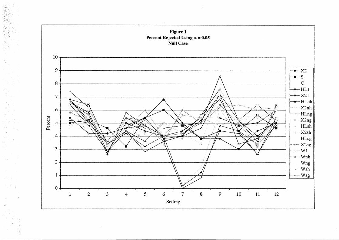
We present in Table 5 the percent of time each of the first 18 statistics denoted in Table 3

rejected the hypothesis of fit at the a= 0.05 level. These empirical alpha levels are plotted

versus the setting number in Figure 1. The plot shows with only a few exceptions the empirical

rejection percents are within two percent of the desired five percent level of significance. The

two partial sum-of-residuals tests that use (x'~r as the omitted covariate and the optimally

weighted partial sum-of-residuals tests using nln(i) as the covariate do not reject often enough

in settings 7 and 8. It is not clear exactly why this is the case; but may it be due to the narrow

;,,,

J:.: '•··- . ,-, ,.'•

11

range in values of the omitted covariate as x-U( -1,1). Further investigations into the reasons

for this behavior are planned.

Power

We use the same three settings used by Hosmer et. al. (1997) to examine the power of the

tests. These are: the omission of a quadratic term in a continuous variable, the omission of the

interaction of a dichotomous variable and a continuous variable and an incorrectly specified link

function. In all settings studied the distribution of the continuous covariate, x, is U( -3,3). The

distribution of the dichotomous covariate, d, is Bernoulli(l/2) and is independent of the

continuous covariate.

We use five different models to evaluate power with omission of a quadratic term from

the model. We generate the outcome variable using a logistic model with logit r(x,~) = /30 + f31x + f32x 2 where the values of the three coefficients are set such that

n(-1.5) = 0.05, n(3) = 0.95 and n(-3) = J for J= 0.01, 0.05, 0.1, 0.2, and 0.4. The linear

logistic model with n(-1.5) = 0.05, n(3) = 0.95 corresponds to a value of J = 0.007. As the J

parameter increases the lack of linearity in the logit function becomes progressively more

pronounced.

We use four different interaction models to study the power with omission of the

dichotomous-continuous interaction term from the model. We generated the outcome variable from a model with logit r(x,d,~) = /30 + f31x + f32d + f33 xd. The four parameters are set such that

n(-3,0) = 0.1, n(-3,1) = 0.1, n(3,0) = 0.2 and n(3,1) = 0.2+1 where 1= 0.1,0.3,0.5,0.7. Thus

the four models display progressively more interaction.

We examine five different models to assess the power to detect an incorrectly specified

link function. We generate the values of the outcome variable from Stukel's generalized logistic

model using the function 'T](X) = 0.8x as the linear predictor and values of the parameters ~ and

a2 as specified in Table 6. Stukel (1988) noted that if~= a2 =0.165 then the resulting

generalized logistic model has nearly the same shape as the probit model. The model with when

~ =0.62 and a2 = -0.037 has the same shape as the complimentary log-log model. We chose

the remaining three situations to yield one model with both tails longer, one model with both

tails shorter tails and an asymmetric model with one tail longer and one tail shorter than the

logistic model.

12

The situations we use to examine the power of the tests were chosen to represent typical

logistic regression models encountered in practice. The combination of two sample sizes, 100

and 500, and the various models examined yields results that further our understanding of what

types of departures from a linear logistic model the various tests can detect with moderate to high

power.

We present in Table 7 the percent of time each of the 24 tests denoted in Table 3 rejected

the hypothesis of fit at the a= 0.05 level.

The results for the quadratic model are presented in Table 7.1 and are plotted versus

setting in Figure 2. We see that the power is, as expected, poor when trying to detect models that·

are quite close to the logistic. As the departure from linearity in the logit increases, the power

increases rapidly. High power is attained for samples of size 100 in those settings where there

are substantial differences over the entire [0,1] interval between the true quadratic model and the

fitted linear model, settings 7 and 9 in Figure 2 where J = 0.20 and J = 0.40. In setting 4 where

J = 0.05 and the sample size is 500 the power is around 80 percent for most tests. In settings 6,

8 and.10 where the sample is size 500 and J ~ 0.1 the power is over 90 percent for all tests. In

settings 5 and 7 where n = 100 and J = 0.1, 0.2 the range in power between the 24 different tests

is nearly 30 percent. The most powerful test, at 65 percent, is the unweighted sum-of-squared

residuals and 11 other tests have power nearly as good, over 55 percent. The least powerful tests

in these as well as most other settings are the unweighted partial sum-of-residuals test and the optimally weighted partial-sum-of-residuals test using omitted covariate irln(n). The pattern of

the test specific polygons in Figure 2 show that power of all the tests increases at about the same

rate as a function of both sample size and deviation from the null model. The power for tests 19

- 24 in Table 3 that use weights optimal for the omitted term, x 2 , have power that is comparable

to but not better than the other tests. In summary, the results in Table 7.1 indicate that when

there is a substantial difference between the linear and quadratic model all tests have high power

and all tests have low power when there is little difference between the fitted and true models.

The results on the power to detect an omitted dichotomous-continuous variable

interaction are presented in Table 7.2 and are plotted versus the setting number in Figure 3. As

can be seen in Figure 3 the power is low, less than about 40 percent, for all tests when the sample

size is 100, settings 1, 3, 5 and 7. One setting where there are important differences in the tests

is setting 6, n = 500 and I= 0.5. The results in Figure 3 show two clusters of tests, ones with

power over 60 percent and those with power less than 50 percent. Among those with power over

60 percent the best four tests are: the partial sum-of-residuals test with optimal omitted covariate,

x x d, and optimal weights, the unweighted sum-of-squared residuals test, the Pearson chi-

13

square statistic and the partial sum-of-residuals test with optimal omitted covariate, x x d, with

approximate optimal weights. As can be seen in Table 7.2 these four tests are the most powerful

in all eight settings. The power is high, over 80 percent, only setting 8 and in setting 6 for the

partial sum-of-residuals test with optimal omitted covariate, x x d, and optimal weights and the

unweighted sum-of-squared residuals test. In summary ,we see that the power to detect the

interaction is generally low. However the new test using the optimal omitted covariate and

optimal weights seems to provide an improvement in power over the less specific tests. We

believe that this improvement in power is important as interactions of the type considered in

these settings are often difficult to detect during model. Any test that can aid in detecting

omitted terms of this type should be used during assessment of model fit.

One exception to the performance of the tests in the quadratic model is the behavior of

the grouped sum-of-residuals tests, HLoh and X2oh, using the optimal omitted covariate and

approximate optimal weights. Further examination of the simulation results of the distribution of

these two tests suggests that the degrees-of-freedom may differ from the values of 8 and 10 used

to compute the significance levels. The results suggest that the degrees-of-freedom may be 6 and

8 respectively. Results, not shown, indicate that power when significance levels are calculated

using 6 and 8 degrees-of-freedom are in line with the other grouped process based tests.

We note that the power results in Table 7.2 indicate substantially better power to detect

an omitted interaction term than results previously in reported in Hosmer et. al. (1997). The

simulations performed here are slightly different in that we fit the model containing both the

continuous and dichotomous covariates while Hosmer ec al.Tit the model only containing the

continuous covariate. We replicated the simulations fitting the model containing only the

continuous covariate and the results were similar to those previously reported. One possible

explanation for the difference in power is that the model one obtains when fitting only fitting the

continuous covariate essentially has a line on the logit scale intermediate between the separate

lines non-parallel lines in the true model. Thus it appears to fit better than a model with two

different parallel lines on the logit scale.

The results for the power to detect an alternative link function are presented in Table 7.3

and plotted versus the setting number in Figure 4. The power is always less than 30 percent for

sample size 100, settings 1, 3, 5, 7 and 9. The only exception is for the asymmetric link function

in setting 9 where the power for the optimally weighted partial sum-of-residuals test using omitted covariate fCln(i) has power of 44.2 percent. The power is over 80 percent only in

setting 10 when n = 500 with the asymmetric link function. In general the results are quite

variable with no single test being optimal in all settings. The unweighted sum-of-squares test

14

performs about the best and has strikingly higher power than all other tests in setting 8, n = 500

and the short tailed link function. As noted in Hosmer et. al. (1997) when both~ and a2 are

large and positive in the Stukel model, the probability function becomes quite steep and the fitted

values, ic, tend to be either small or large. When this occurs the Pearson chi-square and

unweighted sum-of-squares tests approach zero. However, their estimated variances become

quite large due to the range in the fitted values. The normalized goodness-of fit tests tend to be

not significant since the numerator is small and the estimated variance is large. The same holds

true for the various "decile-of-risk" tests. We note that the power of the Pearson chi-square

statistic and the "decile-of-risk" tests in Table 7.3 are less than the riominal alpha level when

lXr = a2 = 1. Although not shown here when the two parameters, CXr and a2 , become sufficiently

large the tests degenerate. However with a sample of size 500 there are a sufficient number of

estimated probabilities that are not near zero or one to allow the unweighted sum-of-squares test

to have a distribution which leads to relatively high power.

In summary, the results in Table 7 and Figure 2- 4 show that overall the goodness-of-fit

tests have reasonable power for detecting a curvature type misspecification of the logit function.

The power is low for sample size 100 to detect an omitted interaction that yields a linear model

with different slopes and an incorrect but still symmetric link function. However, for sample

size 500 several tests had reasonable power to detect a moderately large interaction term.

The overall performance of the Pearson chi-square statistic and unweighted sum-of­

squares statistic was, overall, superior to most tests. The performances of all the "decile-of-risk"

type tests were similar. The performance of the new optimally weighted partial residual sum-of­

residuals test using the optimal covariate shows promise in detecting lack-of-fit due to omitted

interactions. The weighted partial sum-of-residuals test using the generic omitted covariates

irln(ir) and (x'Pt did not have power better than more easily calculated tests.

When we consider computational issues, power and current availability in packages a

practical strategy is to use the Pearson chi-square statistic and/or the unweighted sum-of-squares A

statistics in conjunction with the Hosmer-Lemeshow decile-of-risk statistic, C. We recommend A

obtaining the 2 by 10 table, of observed and estimated expected frequencies used to compute C

as it provides a useful overall summary of the fit or lack-of-fit of the model and is easily

understood by subject matter scientists. In addition, we recommend using the optimally

weighted partial sum-of-residuals test using perhaps several "educated guesses" about possible

omitted covariates, especially interactions, from the model.

·',:'• ' ~ i -·:

', ' ' ' .... ' i~:."' ~

15

;, t''

Return to the Example

We return to an evaluating the fit of the model for low birth weight shown in Table 1.

We present in Table 9 the p-values of al124 tests. These results in show that only one of the 24

tests, X2 sh, hasp< 0.05 and two others have p-values between 0.05 and 0.15. When we

employ the recommended strategy of using the Pearson chi square and/or unweighted sum-of­

squares tests for power against overall non-linearity in the logit, the Hosmer-Lemeshow decile of

risk statistic and 2 by 10 table for confirmatory evidence we see that it suggests overall fit of the

model. The optimally weighted partial sum-of-residuals test using AGE2 as the omitted

covariate yields p = 0.40, further supporting model fit.

Summary

The use of overall summary measures of goodness-of-fit of logistic regression models has

become an important and easily performed step in model building. Decisions on model fit using

tests based on cutpoints may depend on choice of cutpoints. A new class of overall goodness-of­

fit tests based on weighted partial sum-of-residuals tests has been studied via simulation under

both null and alternative scenarios. The simulation results showed that, with a few exceptions,

all tests had the correct size. The optimal weighted partial sum-of-residuals test had the highest

power for omission of a quadratic term. The Pearson chi-square and unweighted sum-of-squares

statistics had power nearly as high. All tests had low power to detect continuous-dichotomous

variable interaction with a small sample size. With a large sample size power was adequate to

detect a moderate interaction for the optimal weighted partial sum-of-residuals test as well as the

Pearson chi -square and unweighted sum of squares test. All tests had more power to detect lack­

of-fit due to model misspecification when the logit was non-monotone increasing (decreasing)

under the alternative than when it was monotone under both null and alternative models. None

of the tests studied had high power to detect an incorrectly specified link function with sample

size 100. Power was high for all tests to detect an asymmetric link function with a sample size of

500 ..

Because of the superior power of the unweighted sum-of-squares statistic and the

Pearson chi-square/unweighted sum-of-squares statistics, we recommend their use. In addition

the optimally weighted partial sum-of-residuals test using one or more choices for an omitted

covariate could be expected to add to the assessment of model fit. We suggest using the decile

of risk tests for confirmation of model fit or lack-of-fit and its associated 2 x 10 table of

observed and estimated expected frequencies as it is easily understood by subject matter

16

scientists. In all cases one must keep in mind the lack of power with small sample sizes to detect

subtle deviations from the logistic model. Thus the choice of both the logistic regression model

and its covariates should have a strong biological or clinical basis.

References

Cook, R.D. and Weisberg, S. Residuals and Influence in Regression, Chapman Hall, New York

NY (1982)

Hosmer, D.W., Hosmer, T., le Cessie, S. and Lemeshow, S. 'A comparison of goodness-of-fit

tests for the logistic regression model', Statistics in Medicine, 16, 965-980 (1997).

Hosmer, D.W. and Lemeshow, S. 'A goodness-of-fit test for the multiple logistic regression

model', Communications in Statistics, A1 0, 1043-1069 (1980).

Hosmer, D.W. and Lemeshow, S. Applied Logistic Regression: Second Edition, John Wiley and

Sons Inc., New York, NY (2000).

Hjort, N.L. Goodness-of-fit tests in models for life history data based on cumulative hazard

rates, Annals of Statistics, 18, 1221-1258 ( 1990).

Hjort, N.L. and Hosmer, D.W. 'Goodness-of-fit processes for logistic regression', Technical

Report, Department of Mathematics and Statistics, University of Oslo, Oslo Norway (2000)

Royston ,P. 'The use of cusums and other techniques in modeling continuous covariates in

logistic regression', Statistics in Medicine, 11, 1115-1129 ( 1992).

Stukel, T.A. 'Generalized logistic models', Journal of the American Statistical Association,

83,426-431 (1988).

Osius, G. and Rojek, D. 'Normal goodness-of-fit tests for multinomial models with large degrees

of freedom', Journal of the American Statistical Association, 8 7,1145-1152 ( 1992).

17

' .. ,_ ·.<··:,I t'.' •

. :··'

Table 1

Estimated Coefficients, Estimated Standard Errors and p­

values from a Model Fit to the Jittered Low Birth Weight

Data

Variable Coefficient Std. Err. p-value

AGEj -0.022 0.0341 0.512

LWTj -0.013 0.0064 0.050

RACE_1 1.232 0.5171 0.017

RACE_2 0.943 0.4162 0.023

SMOKE 1.054 0.3800 0.006

CONSTANT 0.333 1.1085 0.764

Table 2

V aloe of the Pearson Chi Square Statistic, X 2 , and Values

of the Hosmer-Lemeshow Decile of Risk Statistic, C, Computed by Six Different Packages

Statistic Value DF p-value

X2 ~ x2 (183) 180.81 183 0.532 X2 ~Normal 180.81 * 0.667 S ~Normal 36.90 * 0.084

A

LOGXACT's C 13.02 8 0.111 A

SAS's C 10.55 8 0.229 A

SPSS's C 10.54 8 0.229

STATA's C 10.55 8 0.229 A

SYSTAT's C 16.10 8 0.041

Tables Page 1

Table 4

Settings Used to Examine the Null Distribution of the Tests for n = 100 and 500 Distributional Characteristics of the

Logistic Probabilities (n = 100) Covariate Distribution Logistic Coefficients nc1J Q1 Qz Q, n(n)

U(-6,6) f3o = 0,{31 =0.8 0.009 0.083 0.5 0.917 0.991 U( -4.5,4.5) f3o = 0,/31 =0.8 0.029 0.142 0.5 0.858 0.971

U(-3,3) f3o = 0,/31 =0.8 0.087 0.231 0.5 0.769 0.913 U(-1,1) f3o = 0,/31 =0.8 0.313 0.400 0.5 0.600 0.687 xz(4) f3o = -4.9,{31 = 0.65 0.009 0.025 0.062 0.202 0.965

Normal-Bernoulli f3o = 0,{31 =0.8,/3z = -0.8, Model* /33 =ln(2) 0.020 0.288 0.589 0.834 0.989

*: (X1,X2 I D= d),..., N((2d,2d),:E], Var(X1) = Var(X2 ) =6,Cor~Xt. X2 ) = 0.5, D,..., B(0.5)

Tables Page 2

/ ' . . ,·

Test# Test Notation

1 xz 2 s 3 c 4 HLl

5 X2 1 6 HLnh

7 X 2nh

8 HLng

9 X 2ng

10 HLsh

11 X 2sh

12 HLsg

13 X 2sg

14 Wl

15 Wnh

16 Wng

17 Wsh

18 Wsg

19 HLoh

20 X 2oh

21 HLog

22 X 2og

23 Woh

24 Wog

' ~· . }. ' ... '·. . . '. ' ." '

Table 3 Definition of Notation for Test Statistics

Description

Pearson Chi -Square

Unweighted Sum-of-Squares

Hosmer-Lemeshow Decile of Risk

Hosmer-Lemeshow, weights= 1

Full Grouped Chi-Square, weights= 1 Hosmer-Lemeshow, omit cov = itln(il"), approximate weights

Full Grouped Chi-Square, omit cov = il"ln(it), approximate weights Hosmer-Lemeshow, omit cov = itln(it), optimal weights

Full Grouped Chi-Square, omit cov = itln(n), optimal weights Hosmer-Lemeshow, omit cov = g2 , approximate weights

Full Grouped Chi-Square, omit cov = g2 , approximate weights

Hosmer-Lemeshow, omit cov = g2 , optimal weights

Full Grouped Chi-Square, omit cov = g2 , optimal weights

Partial Sums-of-Residuals, weights= 1 Partial Sums-of-Residuals, omit cov = nln(il"), approximate weights

Partial Sums-of-Residuals, omit cov = itln(it), optimal weights Partial Sums-of-Residuals, omit cov = gz, approximate weights

Partial Sums-of-Residuals, omit cov = g2 , optimal weights Hosmer-Lemeshow, model specif. omit cov , approximate weights

Full Grouped Chi-Square, model specif. omit cov, approximate weights

Hosmer-Lemeshow, model specif. omit cov, optimal weights Full Grouped Chi-Square, model specif. omit cov, optimal weights Partial Sums-of-Residuals, model specif. omit cov, approximate weights

Partial Sums-of-Residuals, model specif. omit cov, optimal weights s

Tables Page 3

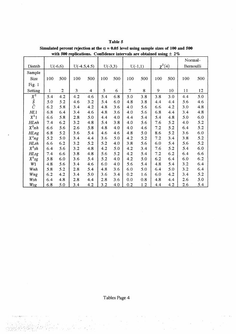
Table 5

Simulated percent rejection at the a= 0.05 level using sample sizes of 100 and 500 with 500 replications. Confidence intervals are obtained using ± 2%

Normal-Distrib U(-6,6) U( -4.5,4.5) U(-3,3) U(-1,1) xz(4) Bernoulli

Sample Size 100 500 100 500 100 500 100 500 100 500 100 500

Fig. 1 Setting 1 2 3 4 5 6 7 8 9 10 11 12

xz 5.4 4.2 4.2 4.6 5.4 6.8 5.0 3.8 3.8 3.0 4.4 5.0 ~ s 5.0 5.2 4.6 3.2 5.4 6.0 4.8 3.8 4.4 4.4 5.6 4.6 A c 6.2 5.8 3.4 4.2 4.8 3.6 4.0 5.6 6.6 4.2 3.0 4.8

HL1 6.8 6.4 3.4 4.6 4.8 3.6 4.0 5.6 6.8 4.4 3.4 4.8 X2 1 6.6 5.8 2.8 5.0 4.4 4.0 4.4 5.4 5.4 4.8 5.0 6.0

HLnh 7.4 6.2 3.2 4.8 5.4 3.8 4.0 5.6 7.6 5.2 4.0 5.2 X 2nh 6.6 5.6 2.6 5.8 4.8 4.0 4.0 4.6 7.2 5.2 6.4 5.2 HLng 6.8 5.2 3.6 5.4 4.6 4.6 4.8 5.0 8.6 5.2 3.6 6.0 xzng 5.2 5.0 3.4 4.4 3.6 5.0 4.2 5.2 7.2 3.4 3.8 5.2 HLsh 6.6 6.2 3.2 5.2 5.2 4.0 3.8 5.6 6.0 5.4 5.6 5.2 X 2sh 6.4 5.6 3.2 4.8 4.2 5.0 4.2 3.4 7.6 5.2 5.4 6.0 HLsg 7.4 6.6 3.8 4.8 5.6 5.2 4.2 5.4 7.2 6.2 6.4 6.6 X 2sg 5.8 6.0 3.6 5.4 5.2 4.0 4.2 5.0 6.2 6.4 6.0 6.2 WI 4.8 5.6 3.4 4.6 6.0 4.0 5.6 5.4 4.8 5.4 3.2 6.4

Wnh 5.8 5.2 2.8 5.4 4.8 3.6 6.0 5.0 6.4 5.0 3.2 6.4 Wng 6.2 4.2 3.4 5.0 3.6 3.4 0.2 1.6 6.0 4.2 3.4 5.2 Wsh 6.4 4.8 2.8 4.4 2.8 3.6 0.0 0.8 4.8 4.4 2.6 5.0 Ws,l? 6.8 5.0 3.4 4.2 3.2 4.0 0.2 1.2 4.4 4.2 2.6 5.4

Tables Page 4

'' J

Table 6 CoeMcients for the Generalized Logistic Model

Model at ~

Pro bit 0.165 0.165

Comp. Log-Log 0.620 -0.037

Long Tails -1.0 -1.0

Short Tails 1.0 1.0

Asymmetric Long-

Short Tails -1.0 1.0

Tables Page 5

,,. ·,·

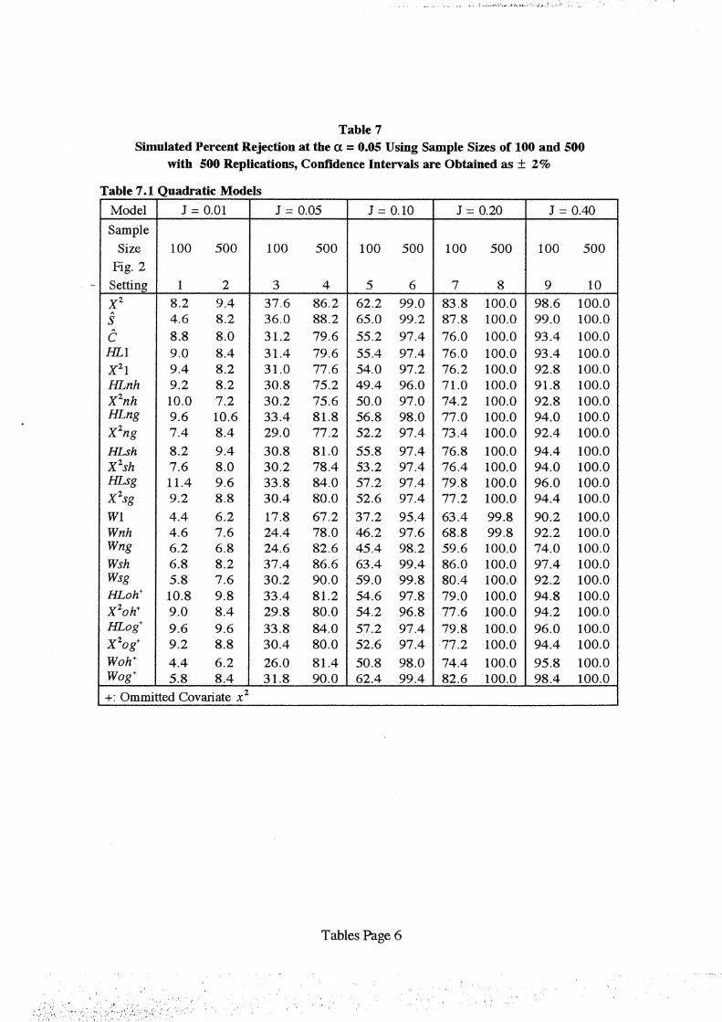
Table 7 Simulated Percent Rejection at the a= 0.05 Using Sample Sizes of 100 and 500

with 500 Replications, Confidence Intervals are Obtained as ± 2%

Table 7.1 Quadratic Models

Model J = 0.01 J = 0.05 J = 0.10 J = 0.20 J = 0.40

Sample

Size 100 500 100 500 100 500 100 500 100 500 Fig. 2

Setting 1 2 3 4 5 6 7 8 9 10 xz 8.2 9.4 37.6 86.2 62.2 99.0 83.8 100.0 98.6 100.0 ~ s 4.6 8.2 36.0 88.2 65.0 99.2 87.8 100.0 99.0 100.0 ~ c 8.8 8.0 31.2 79.6 55.2 97.4 76.0 100.0 93.4 100.0

HL1 9.0 8.4 31.4 79.6 55.4 97.4 76.0 100.0 93.4 100.0 X21 9.4 8.2 31.0 77.6 54.0 97.2 76.2 100.0 92.8 100.0 HLnh 9.2 8.2 30.8 75.2 49.4 96.0 71.0 100.0 91.8 100.0 X 2nh 10.0 7.2 30.2 75.6 50.0 97.0 74.2 100.0 92.8 100.0 HLng 9.6 10.6 33.4 81.8 56.8 98.0 77.0 100.0 94.0 100.0 X 2ng 7.4 8.4 29.0 77.2 52.2 97.4 73.4 100.0 92.4 100.0

HLsh 8.2 9.4 30.8 81.0 55.8 97.4 76.8 100.0 94.4 100.0 X 2sh 7.6 8.0 30.2 78.4 53.2 97.4 76.4 100.0 94.0 100.0 HLsg 11.4 9.6 33.8 84.0 57.2 97.4 79.8 100.0 96.0 100.0 X 2sg 9.2 8.8 30.4 80.0 52.6 97.4 77.2 100.0 94.4 100.0

W1 4.4 6.2 17.8 67.2 37.2 95.4 63.4 99.8 90.2 100.0 Wnh 4.6 7.6 24.4 78.0 46.2 97.6 68.8 99.8 92.2 100.0 Wng 6.2 6.8 24.6 82.6 45.4 98.2 59.6 100.0 74.0 100.0 Wsh 6.8 8.2 37.4 86.6 63.4 99.4 86.0 100.0 97.4 100.0 Wsg 5.8 7.6 30.2 90.0 59.0 99.8 80.4 100.0 92.2 100.0 HLoh+ 10.8 9.8 33.4 81.2 54.6 97.8 79.0 100.0 94.8 100.0 X 2oh+ 9.0 8.4 29.8 80.0 54.2 96.8 77.6 100.0 94.2 100.0 HLog +

9.6 9.6 33.8 84.0 57.2 97.4 79.8 100.0 96.0 100.0 X 2og+ 9.2 8.8 30.4 80.0 52.6 97.4 77.2 100.0 94.4 100.0 Woh+ 4.4 6.2 26.0 81.4 50.8 98.0 74.4 100.0 95.8 100.0 Wog+ 5.8 8.4 31.8 90.0 62.4 99.4 82.6 100.0 98.4 100.0

+: Ommitted Covariate x 2

Tables Page 6

'·, ;J·•'.

''

Table 7.2 Interaction Models

Model I= 0.1 I= 0.30 I = 0.50 I= 0.70

Sample

Size 100 500 100 500 100 500 100 500 Fig. 3

Setting 1 2 3 4 5 6 7 8

~ 5.2 5.6 8.8 29.8 23.0 68.0 38.4 93.8 s 5.6 5.0 8.2 26.8 21.8 72.0 40.2 98.6

A

c 4.6 5.6 5.0 11.4 10.8 40.2 23.2 84.2 HL1 4.6 5.6 5.0 12.0 10.8 40.2 23.2 84.4 X21 5.4 6.0 5.8 12.6 11.8 39.2 23.0 82.2

HLnh 4.6 5.8 5.4 12.0 11.4 38.0 23.4 82.0 X 2nh 5.0 6.0 6.0 12.2 12.2 40.8 25.0 82.6 HLng 5.8 5.6 7.2 13.6 11.8 42.6 26.2 85.8 X 2ng 4.6 5.8 6.6 13.8 10.8 41.2 24.4 84.4 HLsh 5.4 6.0 5.6 12.0 10.6 42.4 23.0 86.4 X 2sh 5.6 5.2 5.6 13.0 11.2 39.6 23.4 85.0 HLsg 6.0 5.4 6.8 12.8 12.2 45.8 27.2 86.4 X 2sg 6.0 5.4 6.4 1.3 10.2 43.8 25.0 84.6 Wl 5.4 5.8 7.2 16.4 13.4 49.8 21.2 86.4

Wnh 3.0 4.8 7.0 18.2 15.8 60.0 26.8 94.6 Wng 0.0 0.4 0.8 10.8 8.4 59.4 27.8 97.0 Wsh 1.6 3.4 3.2 20.8 13.8 61.4 31.8 96.4 Wsg 0.4 0.8 1.6 14.4 8.0 62.6 27.2 97.4

HLoh+ 2.2 3.4 2.4 1.6 1.4 2.2 0.4 10.6 X 2oh- 1.4 3.7 2.6 4.6 2.8 26.8 4.8 71.0 HLog + 5.6 5.0 6.4 14.0 11.8 46.2 26.8 89.0 X 2og 6.0 4.2 6.8 13.2 9.6 43.4 24.0 84.6 Wah+ 7.0 7.6 8.0 23.6 15.8 64.8 29.8 95.2. Wo£ 6.6 8.0 10.6 32.8 24.0 76.4 38.0 98.6

+: Ommitted Covariate x x d

Tables Page 7

'• .'

~ ~. ' •' · .. ' ~ -... \

Table 7.3 Alternative Link Functions

Model Pro bit Comp. Log-Log Long Tails Short Tails Asymmetric Long-

Short Tail

Sample Size 100 500 100 500 100 500 100 500 100 500

Fig. 4 Setting 1 2 3 4 5 6 7 8 9 10

xz 6.4 7.6 2.6 17.6 5.0 13.0 0.4 43.6 2.4 87.2 A s 5.8 10.2 5.2 23.4 5.4 12.6 11.0 77.2 17.8 86.4 A

c 4.8 6.8 3.4 27.0 4.0 7.8 3.4 19.0 12.2 92.6 HL1 5.0 6.8 3.6 27.6 4.0 7.8 3.4 19.2 12.6 92.8 X21 5.0 7.6 4.4 25.4 5.2 7.8 3.0 19.4 11.8 91.8

HLnh 5.6 6.8 4.0 26.2 3.8 7.8 5.0 19.4 12.0 91.8 X 2nh 4.2 7.6 5.4 26.0 4.6 7.0 3.8 16.2 10.2 91.6 HLng 6.2 8.6 6.0 28.0 5.6 8.4 3.2 12.0 13.4 94.0 X 2ng 4.0 8.0 6.6 26.4 4.2 7.8 2.6 19.0 12.0 91.0 HLsh 4.2 7.0 5.6 23.8 4.6 7.4 3.6 17.2 13.0 90.8 X2sh 3.8 6.6 6.0 24.8 3.6 7.8 3.0 17.0 11.0 91.8 HLsg 6.2 9.6 7.0 31.0 6.6 8.2 3.2 13.8 15.0 94.4 X 2sg 4.0 11.2 6.8 25.0 4.4 7.6 2.4 18.4 12.0 92.0 W1 6.0 7.6 9.0 37.6 6.4 8.2 11.0 41.6 25.4 95.0

Wnh 5.8 7.2 8.4 21.4 6.0 8.0 13.4 46.2 28.0 98.0 Wng 5.6 5.2 10.8 36.0 1.4 4.4 7.6 19.6 44.2 99.8 Wsh 3.2 4.0 8.0 48.0 0.0 4.0 10.2 2.6 22.4 99.8 Ws,R" 2.8 4.6 9.6 5.1 0.0 4.0 0.8 2.0 28.8 99.8

Tables Page 8

• . ' .-"'. 1,.

': '. ·,-, I , .. 'r'/-r•·. • -~~. -.·"'~

.::,

Table 8 P-Values ofthe Goodness-of-Fit

Statistics for the Low Birth Weight

Model in Table 1

Statistic p-value x2 0.667

A

s 0.084 A c 0.229

HL1 0.385

X 2 1 0.543

HLnh 0.367

X 2nh 0.498

HLng 0.127

X 2ng 0.239

HLsh 0.340

X 2sh .0446

HLsg 0.147

X 2sg 0.270

W1 0.362

Wnh 0.438

Wng 0.325

Wsh 0.900

Wsg 0.300 HLoh+ 0.359 X 2oh+ 0.520 HLog+ 0.239 X 2og+ 0.053 Woh+ 0.188 Wog+ 0.400

+: Omitted Covariate = AGE/

Tables Page 9

9

8

f\

7 .....

6

~ 8 5 1 ~-"-"~ tu ~~· ..

0...

4j ·~~~

3 y

2

Figure 1 Percent Rejected Using a= 0.05

Null Case

1,-----0 ---------

1 2 3 4 5 6 7 8

Setting

9 10 11 12

····J.i•-·Wnh Wng

--Wsh --Wsg

- ... -

100.0

90.0

80.0

70.0

60.0 +-'

5 50.0 ~ 0..

40.0

30.0

20.0

10.0

0.0

)

1 2 3 4

Figure 2 Percent Rejected Using a. = 0.05

Quadratic Models

5 6 7

Setting

""

-+-X2

-s2 c

~HLl

-*-X21 _,._HLnh

-t--X2nh

-HLng -X2ng

HLsh

X2sh HLsg

--+<~ X2sg

Wl ··.";fr····Wnh

Wng --Wsh

-Wsg

---.-·-- Hloh ;,1;<-X2oh

---·<i·--Hlog ---*- X2og

~Wah

8 9 10 ,-.-wag

' . . ~

100.0

90.0

80.0

70.0

60.0

'· :_; ,,

~

§ 50.0 1-<

~ 40.0

30.0

-~. -'

20.0

10.0

0.0

. -..,_•.

I

-----

1 2 3

Figure 3 Percent Rejected Using a = 0.05

Interaction Models

/

4 5

Setting

./· ·.,,

'•.,

i

6 7

/ /

//

/ / /

~./

8

-+-X2

------ S2 c

~HL1

-.-x21 -+-HLnh -+-X2nh --HLng -X2ng

HLsh X2sh HLsg

_,,*, .. X2sg

<~··W1

.• ,01- .. Wnh

Wng --Wsh --Wsg --+-- Hloh

··i1i~ ·X2oh - &--- Hlog

-*-X2og -.-woh ----.-"-- Wog

100.00

90.00 .. ·'

80.00

- _..::. 70.00

60.00

~ 50.00 8

~ 40.00

30.00

20.00

10.00

0.00 1 2 3

Figure 4 Percent Rejected Using a = 0.05

Alternative Link Models

4 5 6 7

Setting

8 9 10

-+-X2 ---s2

c --*-HLl __._X21 -.-HLnh --t-X2nh --HLng -X2ng

HLsh X2sh HLsg

---J<:--· X2sg ·· :JcW1 ..... .., .. Wnh

Wng -Wsh --Wsg

• - ~' ~· .;------ --c.o·'.-~ ..... , .. ,~_. ......... _~--------