GO-GARCH: a multivariate generalized orthogonal GARCH model

JOURNAL OF APPLIED ECONOMETRICSJ. Appl. Econ. 17: 549–564 (2002)Published online in Wiley InterScience (www.interscience.wiley.com). DOI: 10.1002/jae.688

GO-GARCH: A MULTIVARIATE GENERALIZED ORTHOGONALGARCH MODEL

ROY VAN DER WEIDE*Department of Economics, CeNDEF, University of Amsterdam, Roetersstraat 11, 1018 WB Amsterdam, The Netherlands

SUMMARYMultivariate GARCH specifications are typically determined by means of practical considerations such as theease of estimation, which often results in a serious loss of generality. A new type of multivariate GARCHmodel is proposed, in which potentially large covariance matrices can be parameterized with a fairly largedegree of freedom while estimation of the parameters remains feasible. The model can be seen as a naturalgeneralization of the O-GARCH model, while it is nested in the more general BEKK model. In order to avoidconvergence difficulties of estimation algorithms, we propose to exploit unconditional information first, sothat the number of parameters that need to be estimated by means of conditional information is more thanhalved. Both artificial and empirical examples are included to illustrate the model. Copyright 2002 JohnWiley & Sons, Ltd.

1. INTRODUCTION

The ‘holy grail’ in multivariate GARCH modelling is without any doubt a parameterization ofthe covariance matrix that is feasible in terms of estimation at a minimum loss of generality.The general multivariate GARCH models available parameterize the covariance matrix by a verylarge number of parameters that are hard to estimate, which often leads to convergence difficultiesof estimation algorithms. Therefore, the choice of the multivariate model is often determined bymeans of practical considerations, i.e. the ease of estimation. The strong restrictions are often notbelieved to reflect the ‘truth’, but they are imposed to guarantee feasibility.

Some of the best-known multivariate GARCH models available include the VECH model ofBollerslev and Wooldridge (1988), the constant correlation model of Bollerslev (1990), the factorARCH model of Engle and Rothschild (1990), and the BEKK model studied by Engle and Kroner(1995). For an overview of the multivariate GARCH models, as well as tests for misspecification,see the paper by Kroner and Ng (1998). An extensive survey of empirical applications of time-varying covariance models in finance can be found in Bollerslev, Chou and Kroner (1992). Inparticular the model of Bollerslev (1990) has been a popular choice for modelling high-variatetime series. A test for its assumption of a constant correlation is introduced in a recent paper byTse (2000). Shortly after, both Engle (2002) and Tsui and Tse (2002) generalized the model toallow for time-varying correlations.

A somewhat different approach is the Orthogonal GARCH (O-GARCH) or principal componentsGARCH method. The principal components approach has first been applied in a GARCH-type context by Ding (1994). Shortly after, Alexander and Chibumba (1996) introduced the

Ł Correspondence to: Roy van der Weide, Department of Economics, CeNDEF, University of Amsterdam, Roetersstraat11, 1018 WB Amsterdam, The Netherlands. E-mail: [email protected]/grant sponsor: Netherlands Organization for Scientific Research (NWO).

Copyright 2002 John Wiley & Sons, Ltd. Received 21 November 2001Revised 17 May 2002

550 R. VAN DER WEIDE

strongly related O-GARCH model. Thereafter, O-GARCH has been a popular choice to modelthe conditional covariances of financial data (see e.g. Klaassen, 1999), mainly because the modelremains feasible for large covariances matrices (see e.g. Alexander, 2002). Recently, the modelhas been elaborated along with applications by Alexander (1998, 2001).

The O-GARCH model implicitly assumes that the observed data can be linearly transformed intoa set of uncorrelated components by means of an orthogonal matrix. These unobserved componentscan be interpreted as a set of uncorrelated factors that drive the particular economy or market,similar to that in the Factor (G)ARCH approach of Engle and Rothschild (1990). The orthogonalityassumption, however, appears to be very restrictive. Indeed, if a linkage with a set of uncorrelatedeconomic components exists, why should the associated matrix be orthogonal? The O-GARCHmodel is also known to suffer from identification problems, mainly because estimation of the matrixis entirely based on unconditional information (the sample covariance matrix). For example, whenthe data exhibits weak correlation, the model has substantial difficulties to identify a matrix thatis truly orthogonal (see e.g. Alexander, 2001).

The multivariate GARCH model proposed in this paper can best be seen as a naturalgeneralization of the O-GARCH model. Clearly, orthogonal matrices are very special, and theyreflect only a very small subset of all possible invertible linear maps. The generalized O-GARCHmodel (GO-GARCH) allows the linkage to be given by any possible invertible matrix. Estimationof the matrix requires the use of conditional information, which in turn solves possible identificationproblems.1 The parameters are relatively easy to estimate, so that a substantial increase in thedegrees of freedom is obtained at a very affordable price.

The next section will introduce the generalized Orthogonal GARCH model (GO-GARCH).Estimation is discussed in Section 3. Sections 4 and 5 present some simulation results and anempirical example, respectively. Section 6 concludes.

2. GENERALIZED ORTHOGONAL GARCH

2.1. Notation

In a multivariate GARCH setting, the conditional covariance matrix of the m-dimensional zeromean random variable depends on elements of the information set up to time t � 1, denotedby =t�1. Assume that xt is normally distributed and that its conditional covariance matrix Vt ismeasurable with respect to =t�1, the multivariate GARCH model is then described by:

xtj=t�1 ¾ N �0, Vt� �1�

where we have assumed that xt is second-order stationary so that V D E�Vt� exists. The informationset =t contains both lagged values of the squares and cross-products of xt and elements of theconditional covariance matrices up to time t, i.e. lagged values of Vt. The challenge in multivariateGARCH modelling is to find a parameterization of Vt as a function of =t�1 that is fairly generalwhile feasible in terms of estimation.

In the following we will frequently use the terms conditional information and unconditionalinformation. We specify unconditional information as information that can be extracted from the

1 For example, the data is not required to exhibit strong correlation for the method to work.

Copyright 2002 John Wiley & Sons, Ltd. J. Appl. Econ. 17: 549–564 (2002)

GO-GARCH: A MULTIVARIATE GARCH MODEL 551

unconditional covariance matrix. By conditional information we mean the information set =t asintroduced above.

2.2. Representation

The key assumption of the GO-GARCH model is the following:

Assumption 1 The observed economic process fxtg is governed by a linear combination ofuncorrelated economic components2 fytg:

xt D Zyt �2�

The linear map Z that links the unobserved components with the observed variables is assumed tobe constant over time, and invertible.

Without loss of generality,3 we normalize the unobserved components to have unit variance,so that:

V D ExtxTt D ZZT �3�

An explicit example, which we will denote the GO-GARCH(1,1) model, would be:

xt D Zyt yt ¾ N�0, Ht� �4�

where each component is described by a GARCH(1,1) process:

Ht D diag�h1,t, . . . , hm,t� �5�

hi,t D �1 � ˛i � ˇi� C ˛iy2i,t�1 C ˇihi,t�1 i D 1, . . . , m �6�

where H0 D I equals the unconditional covariance matrix of the components.4 The conditionalcovariances of fxtg are given by:

Vt D ZHtZT �7�

2.3. Identification

Let P and denote the matrices with, respectively, the orthonormal eigenvectors and theeigenvalues of the unconditional covariance matrix V D ZZT.

2 Note that there might be more components than the number of variables observed, so that exposing a set of reliablecomponents could be troublesome. However, if the components are assumed to be described by independent GARCH-typemodels, a new set of uncorrelated components can be constructed by aggregating the ‘original’ components. Under certainconditions, the (extracted) aggregated components are also described by GARCH-type processes. See, for example, Drostand Nijman (1993) in which temporal aggregation of GARCH processes is considered. However, it is known that theGARCH-type ‘features’ typically become weaker under aggregation. As a consequence, the accuracy with which thecomponents are described by GARCH-type models increases as more components can be extracted, which will result inbetter fits.3 Note that the unconditional variances of the components and the matrix Z are directly related. Let fytg denote thecomponents with original scaling, and let the normalized set of components be denoted by fQytg, so that fQytg D fDytg,where D represents the diagonal normalization matrix. The observed process is then given by fxtg D fZytg D f QZ Qytg, whereQZ D ZD�1.4 Ling and McAleer (2002) provide a method for treating the initial value when it comes to asymptotic theory formultivariate GARCH.



Let us assume that an orthogonal linear linkage Z indeed exists, so that xt D Zyt. Theunconditional covariance matrix V is then given by: V D ZHZT, where H is diagonal. Thenthe orthogonal matrix P, the O-GARCH estimator for Z, is only guaranteed to coincide with Z,when the diagonal elements of H are all distinct. Identification problems thus arise when someof the uncorrelated components have similar unconditional variance. To see this, suppose that allcomponents have unit variance, so that V D ZIZT D I. Clearly, the matrix Z is no longer identifiedby the eigenvector matrix of V, as for every orthogonal matrix Q, we have �ZQ��ZQ�T D I. Notethat the eigenvalues of V reflect the variances of the components when the model is well identified.The estimations should therefore be interpreted with caution when some of the eigenvalues arealmost identical. Problems of this type are known to occur when, for example, the data exhibitsweak dependence.5 The next lemma states that the linkage Z is well identified when conditionalinformation is taken into account.

Lemma 2 Let Z be the map that links the uncorrelated components fytg with the observed processfxtg. Then there exists an orthogonal matrix U0 such that:

P12 U0 D Z �8�

Proof. The result follows directly from Singular Value Decomposition, see e.g. Horn andJohnson (1999). �

Let the estimator for U0 be denoted by U. Without loss of generality, we restrict the determinantof U to be 1.6

It can be verified that the orthogonal matrices P and have [m�m � 1�]/2 and m degreesof freedom, respectively. Together with the [m�m � 1�]/2 degrees of freedom for U, we havem C m�m � 1� D m2 degrees of freedom for the invertible matrix Z. The matrices P and willbe estimated by means of unconditional information, as they will be extracted from the samplecovariance matrix V. Conditional information is required to estimate U0.

Note that there is a continuum of matrices Q for which a set of linearly independent componentsut D Qxt can be obtained. For every choice of orthogonal matrix U, the linear transformation

Q D UT� 12 PT induces an uncorrelated series with unit variance: EutuT

t D QVQT D UTU D I.Clearly, these components often still exhibit a form of non-linear correlation. Therefore, linearindependence can be very deceiving, as it might give the impression that the linkage between theobserved variables and the uncorrelated components is uncovered, when more often it is not. Theoriginal components can only7 be restored by means of the inverse of Z.

According to Lemma 2, the model is well identified as there exists a U0 that is associated withthe original Z. Indeed, the additional [m�m � 1�]/2 degrees of freedom induced by the extra termU extends the representation to full generality, in the sense that any invertible linkage Z can inprinciple be estimated from the data, instead of orthogonal matrices only.

5 Given that the observed data is normalized to have unit variance, which is common practice.6 More precisely, U is considered an element of SO(m), which denotes the set of all m-dimensional orthogonal matriceswith positive determinant.7 Equivalent matrices, in the sense that they only exchange variables, for example, are included.



One way to parameterize the estimator for the orthogonal matrix U0 would be by means ofrotation matrices.8

Lemma 3 Every m-dimensional orthogonal matrix U with det�U� D 1 can be represented as aproduct of

(m2

) D [m�m � 1�]/2 rotation matrices:

U D∏i<j

Rij��ij� � � � �ij � � �9�

where Rij��ij� performs a rotation in the plane spanned by ei and ej over an angle �ij.

Proof. See Vilenkin (1968). �

The rotation angles9 f�ijg are commonly referred to as the Euler angles, which can be estimatedby means of maximum likelihood.

We have noted earlier already that the O-GARCH model suffers from identification problems,for example when the data exhibits weak correlation. These problems should not arise whenconditional information is exploited, as proposed in the GO-GARCH model. For example, whenthe uncorrelated components appear to be observed directly, we expect the estimator for U0 to

be close to PT, since OZ D P12 PT D V

12 is approximately diagonal when the data is virtually

uncorrelated.

2.4. Time-varying Correlations

The implied conditional correlations fRtg of the observed process fxtg can be computed as:

Rt D D�1t VtD

�1t Dt D �Vt°I�

12 �10�

where fVtg D fZHtZTg denotes the conditional covariances of fxtg D fZytg, and where ° denotesthe Hadamard product.

This theoretical example illustrates how possible lower and upper bounds for the correlationdepend on the type of linear map Z. Let Z� be the following two-dimensional map:

Z� D(

1 0cos � sin �

)�11�

where � measures the extent to which the uncorrelated components are mapped in the samedirection. For � D 0 the map is not invertible yielding perfect correlation between the observedvariables, whereas for � D 1

2 � we have the identity map, so that the observed variables arecompletely uncorrelated. Let the conditional variances of the uncorrelated components be denoted

8 An alternative parameterization of the orthogonal matrix can be found in van der Weide (2002).9 Note that the values for the angles will depend on the ordering of the rotation matrices. The ordering should not affectthe estimation results.



by �h1t, h2t�. It can be verified that the conditional correlation between the observed variables,denoted by �t, is given by:

�t D h1t cos �√h1t

√h1t cos2 � C h2t sin2 �

�12�

If we assume that hit > 0, we can define zt D h2t/h1t, so that �t can be expressed as:

�t D 1√1 C zt tan2 �

�13�

For finite samples, the variable zt will have finite lower and upper bounds. As a consequence, theconditional correlation �t is also bounded.

Note that a constant linkage Z� gives rise to time-varying correlations between the observedvariables. These correlations rise on average when the components are mapped more in the samedirection. We can not exclude the possibility that the ‘economic mechanism’ Z evolves overtime. If so, endogenizing Z and making it time-varying might improve the fit of the time-varyingcorrelations. Extending the GO-GARCH model to allow for a non-constant Z, however, is left forfurther research. A first step would be to test for a constant linkage, for example by means of teston structural change such as the Chow test.

3. ESTIMATION

The parameters that need to be estimated by means of conditional information, include the vector� of rotation coefficients that will identify the invertible matrix Z (see Lemma 2-3), and theparameters �˛, ˇ� for the m univariate GARCH(1,1) specifications. The log likelihood L�,˛,ˇ forthe GO-GARCH model can be represented as:

L�,˛,ˇ D �1

2

∑t

m log�2�� C log jVtj C xTt V�1

t xt �14�

D �1

2

∑t

m log�2�� C log jZ�HtZT� j C yT

t ZT� �Z�HtZ

T� ��1Z�yt �15�

D �1

2

∑t

m log�2�� C log jZ�ZT� j C log jHtj C yT

t H�1t yt �16�

where Z�ZT� D PPT is independent of �. For the initial value of Ht we take the identity matrix,

which equals the implied unconditional covariance of fytg. Even in high-variate cases, when thecovariance matrices are very large, it should not be a problem to maximize the log likelihoodover the [m�m � 1�]/2 C 2m parameters. Note that in order to avoid convergence difficultiesof estimation algorithms, we propose a kind two-step estimation. We exploit unconditionalinformation first, so that the number of parameters for Z that are estimated through maximumlikelihood is [m�m � 1�]/2 instead of m2 (see lemma 2).

3.1. Consistency

Conditions for strong consistency of the maximum likelihood estimator for general multivariateGARCH are derived by Jeantheau (1998). These conditions are verified by Comte and Lieberman



(2001) for the general BEKK model, in which a result of Boussama (1998), concerning theexistence of a stationary and ergodic solution to the multivariate GARCH(p, q) process, is used.

It can be verified that the more general BEKK model has the GO-GARCH model nested as aspecial case (see van der Weide, 2002). Strong consistency of the quasi MLE for GO-GARCH cantherefore be established by appealing to Jeantheau’s conditions, following Comte and Lieberman.To keep it simple, we focus on the GO-GARCH(1,1) model as in (4), but it can be verified that theresults also hold for the more general GO-GARCH(p,q) model. To apply the results of Jeantheau(1998), we assume that the starting value of the process is drawn from its stationary distributionP�0 , although Comte and Lieberman (2001) indicate that consistency holds for an arbitrary startingvalue. We refer to Ling and McAleer (2002) for a more extensive discussion of the treatment ofthe initial value and its implication for asymptotic properties.

Proposition 4 Consider the GO-GARCH(1,1) model, where ˛i and ˇi denote the GARCH(1,1)parameters of the independent components. If the components are stationary, i.e.

˛i C ˇi < 1 for i D 1, . . . , m �17�

then the MLE is consistent.

Proof. The result follows directly from the derivation of Comte and Lieberman (2001). �

How to conduct inference is beyond the scope of this paper. However, as Comte and Lieberman(2001) have proven asymptotic normality of the quasi-MLE for the BEKK model, having GO-GARCH nested as a special case, we conjecture that this property is also inherited by GO-GARCH.Some caution will be in place though, since we proposed a kind of two-step estimation which willaffect the distribution of the estimator. For example, the standard errors might be underestimatedby the Fisher Information matrix. We leave a precise study of the asymptotic distribution forfurther work. For tests on possible misspecification of the multivariate GARCH model see Kronerand Ng (1998), and the more recent paper by Tse (2002).

4. SIMULATION RESULTS

This section aims to illustrate the behaviour of the GO-GARCH model by experimenting withartificial data.

4.1. Orthogonal Linkage

We constructed the independent components by generating from four univariate GARCH(1,1)models to build a four-variate time series. The conditional variance of each component isdescribed by:

hi,t D ci C ˛iy2i,t�1 C ˇihi,t�1 i D 1, . . . 4 �18�

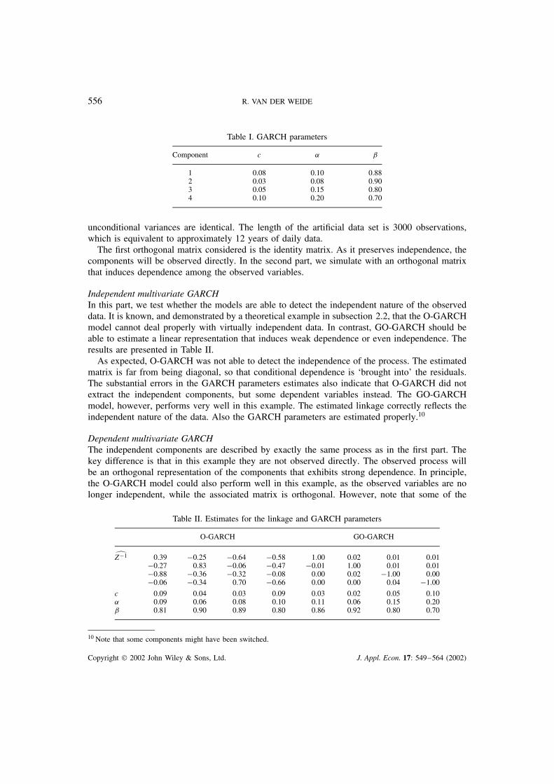
The values that are assigned to the parameters �c, ˛, ˇ� are summarized in Table I.The parameters are chosen so that variances are nearly integrated, which is commonly observed

in financial data. Also note that the parameters are chosen in such a way that some of the



Table I. GARCH parameters

Component c ˛ ˇ

1 0.08 0.10 0.882 0.03 0.08 0.903 0.05 0.15 0.804 0.10 0.20 0.70

unconditional variances are identical. The length of the artificial data set is 3000 observations,which is equivalent to approximately 12 years of daily data.

The first orthogonal matrix considered is the identity matrix. As it preserves independence, thecomponents will be observed directly. In the second part, we simulate with an orthogonal matrixthat induces dependence among the observed variables.

Independent multivariate GARCHIn this part, we test whether the models are able to detect the independent nature of the observeddata. It is known, and demonstrated by a theoretical example in subsection 2.2, that the O-GARCHmodel cannot deal properly with virtually independent data. In contrast, GO-GARCH should beable to estimate a linear representation that induces weak dependence or even independence. Theresults are presented in Table II.

As expected, O-GARCH was not able to detect the independence of the process. The estimatedmatrix is far from being diagonal, so that conditional dependence is ‘brought into’ the residuals.The substantial errors in the GARCH parameters estimates also indicate that O-GARCH did notextract the independent components, but some dependent variables instead. The GO-GARCHmodel, however, performs very well in this example. The estimated linkage correctly reflects theindependent nature of the data. Also the GARCH parameters are estimated properly.10

Dependent multivariate GARCHThe independent components are described by exactly the same process as in the first part. Thekey difference is that in this example they are not observed directly. The observed process willbe an orthogonal representation of the components that exhibits strong dependence. In principle,the O-GARCH model could also perform well in this example, as the observed variables are nolonger independent, while the associated matrix is orthogonal. However, note that some of the

Table II. Estimates for the linkage and GARCH parameters

O-GARCH GO-GARCH

Z�1 0.39 �0.25 �0.64 �0.58 1.00 0.02 0.01 0.01�0.27 0.83 �0.06 �0.47 �0.01 1.00 0.01 0.01�0.88 �0.36 �0.32 �0.08 0.00 0.02 �1.00 0.00�0.06 �0.34 0.70 �0.66 0.00 0.00 0.04 �1.00

c 0.09 0.04 0.03 0.09 0.03 0.02 0.05 0.10˛ 0.09 0.06 0.08 0.10 0.11 0.06 0.15 0.20ˇ 0.81 0.90 0.89 0.80 0.86 0.92 0.80 0.70

10 Note that some components might have been switched.



components have a similar scaling (unconditional variance). As a consequence, O-GARCH mightstill suffer from identification problems, see subsection 2.2.

The orthogonal matrix, denoted by Z, is constructed as a product of four rotation matrices, andis shown in Table III. Table IV summarizes the results.

In the case of O-GARCH, the estimates for the GARCH parameters are clearly differentfrom the true parameters suggesting that the model was not able to identify the independentcomponents. In the previous subsection we have seen that the trivial orthogonal matrix, namelyidentity, could also not be identified by O-GARCH. Thus even when the linkage is trulyorthogonal, there is no guarantee that O-GARCH is able to identify it. The model additionallyrequires that all the components have a different scaling, which might often not be the case (seesubsection 2.2).

When we look at the estimates of the GO-GARCH model, we find that the GARCH parametersof the components are estimated with reasonable accuracy.11 From this we conclude that thelinkage estimated by GO-GARCH cannot be far from the ‘truth’ as we build it.

4.2. Non-orthogonal Invertible Linkage

In this subsection, non-orthogonal invertible matrices are chosen to link the independent com-ponents with the observed process. This will be an important example, as we generalized theO-GARCH model to be able to expose linkages that are not orthogonal. Note that in section 3.3it was illustrated with a theoretical example that lower bounds for the conditional correlations canbe observed when the matrices approach singularity.

In order to have a more controlled experiment, we confine ourselves to the two-dimensionalcase. Similar to the first examples, we construct two independent components in order to build up

Table III. Orthogonal linkage

Map Z

Matrix

p3

2p

2� 1

212 � 1

2p

2p3

2p

212 � 1

2 � 12p

2

�p

34

12p

21

2p

2� 3

4

14

p3

2p

2

p3

2p

2

p3

4

Table IV. Estimates for the GARCH parameters

O-GARCH GO-GARCH

c 0.05 0.08 0.05 0.07 0.10 0.02 0.05 0.03˛ 0.06 0.07 0.07 0.06 0.20 0.06 0.15 0.11ˇ 0.89 0.84 0.89 0.87 0.70 0.92 0.80 0.86

11 Note that some components have been switched.



Table V. The GARCH parameters

Component c ˛ ˇ

1 0.05 0.15 0.802 0.05 0.25 0.70

Table VI. The invertible linkages

Map Z1 Z2 Z3 Z4

Matrix(

1 10 1

) (12 1

0 2

) (2 �21 1

) (1 22 1

)

Table VII. The unconditional covariances

Map Z1 Z2 Z3 Z4

Vi

(2 11 1

) (54 2

2 4

) (2 11 5

) (5 44 5

)

Table VIII. The true linear representations

Map Z1 Z2 Z3 Z4

Wi

(1.41 �1

0 1

) (2.24 �2

0 1

) (0.47 0.75

�0.94 0.75

) ( �0.75 1.491.49 �0.75

)

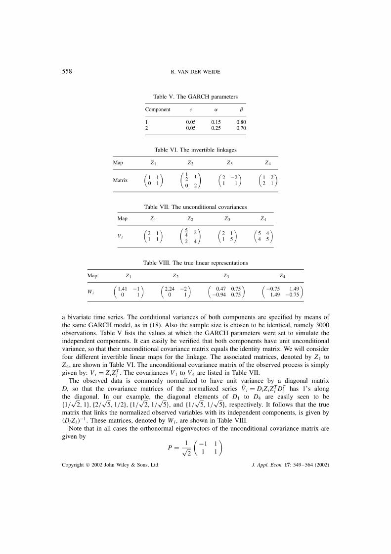
a bivariate time series. The conditional variances of both components are specified by means ofthe same GARCH model, as in (18). Also the sample size is chosen to be identical, namely 3000observations. Table V lists the values at which the GARCH parameters were set to simulate theindependent components. It can easily be verified that both components have unit unconditionalvariance, so that their unconditional covariance matrix equals the identity matrix. We will considerfour different invertible linear maps for the linkage. The associated matrices, denoted by Z1 toZ4, are shown in Table VI. The unconditional covariance matrix of the observed process is simplygiven by: Vi D ZiZT

i . The covariances V1 to V4 are listed in Table VII.The observed data is commonly normalized to have unit variance by a diagonal matrix

D, so that the covariance matrices of the normalized series QVi D DiZiZTi DT

i has 1’s alongthe diagonal. In our example, the diagonal elements of D1 to D4 are easily seen to bef1/

p2, 1g, f2/

p5, 1/2g, f1/

p2, 1/

p5g, and f1/

p5, 1/

p5g, respectively. It follows that the true

matrix that links the normalized observed variables with its independent components, is given by�DiZi��1. These matrices, denoted by Wi, are shown in Table VIII.

Note that in all cases the orthonormal eigenvectors of the unconditional covariance matrix aregiven by

P D 1p2

( �1 11 1

)Copyright 2002 John Wiley & Sons, Ltd. J. Appl. Econ. 17: 549–564 (2002)


Table IX. The estimates for the linkages and the GARCH parameters

Map O-GARCH

Z1 Z2 Z3 Z4

OWi 0.54 0.54 0.51 0.51 �0.61 �0.61 0.53 0.531.31 �1.31 2.17 �2.17 0.86 �0.86 1.59 �1.59

Oci 0.06 0.05 0.05 0.05 0.05 0.05 0.05 0.06O i 0.18 0.12 0.21 0.13 0.14 0.23 0.11 0.12O i 0.76 0.83 0.73 0.82 0.82 0.72 0.84 0.81

Table X. The estimates for the linkages and the GARCH parameters

Map GO-GARCH

Z1 Z2 Z3 Z4

OWi 0.01 0.99 0.02 0.98 �0.48 �0.73 1.49 �0.741.41 �1.01 2.23 �2.00 0.94 �0.76 0.77 �1.51

Oci 0.05 0.05 0.05 0.05 0.05 0.05 0.05 0.05O i 0.25 0.14 0.25 0.14 0.14 0.25 0.25 0.14O i 0.71 0.81 0.71 0.81 0.81 0.71 0.71 0.81

so that O-GARCH is expected to estimate scaled versions of P for the linkages. The results forboth the O-GARCH and the GO-GARCH model are presented in Table IX and X, respectively.

This example illustrates that the GO-GARCH model is able to deal with decompositions thatare not of the orthogonal type. The estimated linkages are in all cases very close12 to the ‘truth’,the matrices from Table VIII. The estimates for the GARCH parameters are also accurate.

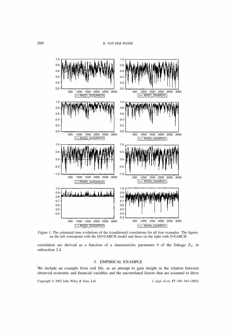
A priori we know that the O-GARCH model cannot uncover the non-orthogonal linkages, asit restricts the matrix to be orthogonal. As a consequence, it extracts components that are notindependent, which is reflected by the biased estimates for the GARCH parameters. Particularlyin example 4, the O-GARCH estimates for the GARCH parameters show substantial error. Thedifference between the estimated correlations is therefore most notable in Example 4, which canbe seen in Figure 1.

In example 4, the GO-GARCH estimates for the correlations never fall below 0.8, say,whereas the correlations estimated by O-GARCH show much stronger declines and some-times even drop to below 0.4. The reason for this effect is that the matrix from example 4shows the strongest ‘deviation’ from an orthogonal matrix. The linkage from example 4 mapsboth independent components in almost the same direction which induces a strong correlationbetween the observed variables. Exactly the same feature is observed in the empirical exam-ple described in the next section. Indeed, it seems reasonable that observed variables that arestrongly related exhibit high correlation at all times. As the linkage with the components thatinduces the high correlation is assumed constant over time, it will be surprising to observeperiods in time where the variables suddenly appear almost uncorrelated. This feature is illus-trated by a theoretical bivariate example, where the lower bound and upper bounds of the

12 Neglect signs, as they do not yield a different representation. Also note that some components might have been switched.



1.0

0.0500 1000 1500 2000 2500 3000

500 1000 1500 2000 2500 3000

500 1000 1500 2000 2500 3000

500 1000 1500 2000 2500 3000

0.2

0.4

0.6

0.8

1.0

0.0

0.2

0.4

0.6

0.8

1.0

-1.0

-0.5

0.0

0.5

1.0

0.4

0.5

0.7

0.6

0.8

0.9

RHO1_GOGARCH

RHO2_GOGARCH

RHO3_GOGARCH

RHO4_GOGARCH

1.0

0.0500 1000 1500 2000 2500 3000

0.2

0.4

0.6

0.8

1.0

0.0500 1000 1500 2000 2500 3000

0.2

0.4

0.6

0.8

1.0

-1.0500 1000 1500 2000 2500 3000

-0.5

0.0

0.5

1.0

0.40.3

500 1000 1500 2000 2500 3000

0.5

0.7

0.6

0.8

0.9

RHO3_OGARCH

RHO1_OGARCH

RHO2_OGARCH

RHO4_OGARCH

Figure 1. The estimated time evolutions of the (conditional) correlations for all four examples. The figureson the left correspond with the GO-GARCH model and those on the right with O-GARCH

correlation are derived as a function of a characteristic parameter � of the linkage Z� , insubsection 2.4.

5. EMPIRICAL EXAMPLE

We include an example from real life, as an attempt to gain insight in the relation betweenobserved economic and financial variables and the uncorrelated factors that are assumed to drive



the market. Our example considers the Dow Jones Industrial Average (DJIA) versus the NASDAQcomposite. The sample contains more than ten years of daily observations, starting on 1 January1990 and ending in October 2001. First, we estimate a first-order13 vector autoregressive (VAR)model to account for the linear structure present in the data. Subsequently, we use the residuals toestimate the conditional covariances from which the (conditional) correlations between the DJIAand the NASDAQ can be computed. Questions that arise naturally include: (i) are non-orthogonallinkages common in real-life examples? (ii) will allowing for a more general linkage (all invertiblematrices) typically induce a better description of the time-varying correlations between economicand financial variables?

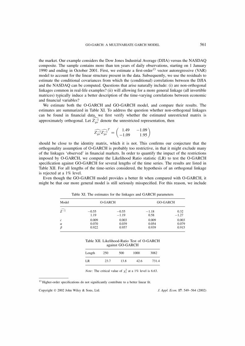
We estimate both the O-GARCH and GO-GARCH model, and compare their results. Theestimates are summarized in Table XI. To address the question whether non-orthogonal linkagescan be found in financial data, we first verify whether the estimated unrestricted matrix isapproximately orthogonal. Let Z�1

go denote the unrestricted representation, then

Z�1go Z�1

go

T D(

1.49 �1.09�1.09 1.95

)should be close to the identity matrix, which it is not. This confirms our conjecture that theorthogonality assumption of O-GARCH is probably too restrictive, in that it might exclude manyof the linkages ‘observed’ in financial markets. In order to quantify the impact of the restrictionsimposed by O-GARCH, we compute the Likelihood Ratio statistic (LR) to test the O-GARCHspecification against GO-GARCH for several lengths of the time series. The results are listed inTable XII. For all lengths of the time-series considered, the hypothesis of an orthogonal linkageis rejected at a 1% level.

Even though the GO-GARCH model provides a better fit when compared with O-GARCH, itmight be that our more general model is still seriously misspecified. For this reason, we include

Table XI. The estimates for the linkages and GARCH parameters

Model O-GARCH GO-GARCH

Z�1 �0.55 �0.55 �1.18 0.321.19 �1.19 0.58 �1.27

c 0.009 0.003 0.009 0.003˛ 0.070 0.039 0.054 0.079ˇ 0.922 0.957 0.939 0.915

Table XII. Likelihood-Ratio Test of O-GARCHagainst GO-GARCH

Length 250 500 1000 3082

LR 23.7 13.8 42.6 731.4

Note: The critical value of �21 at a 1% level is 6.63.

13 Higher-order specifications do not significantly contribute to a better linear fit.



Table XIII. Misspecification test: VAR model on the squares and the product of thetwo residuals

Model Variable O-GARCH GO-GARCH

ε21,t ε2

2,t ε1,tε2,t ε21,t ε2

2,t ε1,tε2,t

c 4.11 4.29 4.22 3.55 4.39 3.89ε2

1,t�1 1.40ŁŁ 0.08 �0.27ŁŁ 1.09Ł 0.52 0.70ε2

2,t�1 1.06ŁŁ 0.36 �0.09 0.92 0.90 0.81ε1,tε2,t �2.44ŁŁ �0.44 0.36 �1.99Ł �1.46 �1.52

adj.R2 0.14 0.00 0.01 0.00 0.00 0.00

Note: Ł,ŁŁ significant at the 5% and 1% level.

a simple test for misspecification. Since we are interested in heteroskedasticity in particular, weestimate a VAR model on the squares and the product of the two standardized residuals to verifywhether the conditional covariance has been modelled correctly. The results, which are shownin Table XIII, suggest that GO-GARCH is not seriously misspecified. The remaining structurefound in the standardized GO-GARCH residuals is fairly weak. In contrast, the residuals from theO-GARCH model still seem to exhibit significant persistence in volatility.

To examine to what extent the restrictions on the linkage affect the (conditional) correlations, wecompare the implied correlations of both models. The time evolution of the correlations is shownin Figure 2, which reveals several interesting features. Perhaps most striking is that the correlationsestimated by GO-GARCH are much less volatile. Furthermore, the GO-GARCH correlations neverseem to fall below 0.6, say, whereas the more volatile correlations estimated by O-GARCH showseveral substantial drops. In the beginning of 2000, the correlation according to O-GARCH iseven just below zero where the GO-GARCH correlations show no decline at all. Since the matrixestimated by GO-GARCH is explicitly not orthogonal, we have reason to believe that O-GARCHoften underestimates the correlations (see subsection 2.4). Indeed, it seems plausible that the DJIAand the NASDAQ, which are strongly related, exhibit high correlation at all times. Assuming thatthe linkage does not change over time, it will be surprising to observe periods where the DJIA andthe NASDAQ appear to be almost unrelated. The differences observed for the year 2000, however,

Figure 2. The estimated correlations between the DJIA and the NASDAQ



are kind of extreme. This might suggest that the linkage is not constant over time, or stronger,that it was subject to a structural change. Indeed, at the beginning of 2000 we experienced atechnological boom which could explain our findings. To test the assumption of a constant linkagewill be left for further research.

6. CONCLUDING REMARKS

A new type of multivariate GARCH model is proposed that can best be seen as a generalizationof the O-GARCH model. It supports the assumption that the observed variables are driven bysome unobserved uncorrelated components, linked by a linear map. In order to identify thesecomponents, we only need invertibility of the associated matrix. Under the null of O-GARCH,however, the matrix is assumed orthogonal which only covers a very small subset of all possibleinvertible matrices. Moreover, even when the matrix is truly orthogonal, the estimator proposedby O-GARCH is not always able to identify it. The GO-GARCH model considers every invertiblematrix as a possible linkage, which will be parameterized in such a way that it is not expected tocomplicate estimation while excluding any identification problems.

The model is tested on both artificial and financial data. The simulation results show that themodel correctly estimates both orthogonal and non-orthogonal invertible linkages. The results arenot affected by the scaling of the uncorrelated factors or a possible weak dependence among theobserved variables. The latter is known to be responsible for the identification problems of O-GARCH, which is confirmed by our experimental results. The nature of the linkage, for examplewhether it is orthogonal or not, is strongly related with the implied correlations between theobserved variables. This relation is made explicit by a theoretical example, and illustrated bysome of the simulation results. The effect of the linkage on the correlations is also observedin the empirical example, the Dow Jones Industrial Average versus the NASDAQ. A likelihoodratio test rejects the hypothesis that the associated matrix is orthogonal. In addition a simple testfor misspecification suggests that the GO-GARCH model provides a better description of theprocess, and the conditional correlations in particular. We argue that by restricting the matrix tobe orthogonal, O-GARCH will often underestimate the correlations. The differences are kind ofextreme during the year 2000, which coincides with the technology boom that initiated early thatyear. It could be that the linkage is not constant over time and that it experienced a structuralchange during the technological bust in 2000. A test for such a structural break, and perhaps evenextending the model to allow for a time-varying linkage, is left for further research. Probablythe most important question that remains is to what extent GO-GARCH is able to improve themodelling of very large covariance matrices. Indeed, it would be very interesting to comparethe model with other recently developed multivariate GARCH models, such as the DynamicConditional Correlation model of Engle (2002). The misspecification tests recently proposed byTse (2002) can be used to measure performance.

ACKNOWLEDGEMENTS

An earlier version of this paper has been presented at the International Conference on Modellingand Forecasting Financial Volatility, Perth, Western Australia, 7–9 September 2001. Stimulatingdiscussions with participants, in particular Robert Engle and the organizers Philip Hans Fransesand Michael McAleer, are gratefully acknowledged. I am especially grateful to Peter Boswijk,



Cees Diks, Roald Ramer and two anonymous referees as they provided helpful comments andsuggestions. I also thank Cars Hommes and Carol Alexander for reading preliminary versionsof the paper. This research has been supported by the Netherlands Organization for ScientificResearch (NWO) under a NWO-MaG Pionier grant. None of the above are responsible for errorsin this paper.

REFERENCES

Alexander C. 1998. Volatility and correlation: Methods, models and applications. In Risk Management andAnalysis: Measuring and Modelling Financial Risk. John Wiley: New York; 125–172.

Alexander C. 2001. Orthogonal GARCH. In Mastering Risk. Financial Times–Prentice Hall: London; 2:21–38.

Alexander C. 2002. Principal component models for generating large GARCH covariance matrices. Reviewof Banking, Finance and Monetary Economics (forthcoming).

Alexander C, Chibumba A. 1996. Multivariate orthogonal factor GARCH. University of Sussex DiscussionPapers in Mathematics.

Bollerslev T. 1990. Modelling the coherence in short-run nominal exchange rates: A multivariate generalizedARCH approach. Review of Economics and Statistics 72: 498–505.

Bollerslev T, Chou RT, Kroner K. 1992. ARCH modeling in finance: A selective review of the theory andempirical evidence. Journal of Econometrics 52: 5–59.

Bollerslev T, Engle RT, Wooldridge J. 1988. A capital asset pricing model with time varying covariances.Journal of Political Economy 96: 116–131.

Boussama F. 1998. Ergodicity, Mixing and Estimation in GARCH Models. PhD dissertation, University Paris7.

Comte F, Lieberman O. 2001. Asymptotic theory for multivariate GARCH processes. Working Paper,CREST-ENSAE, Paris.

Ding Z. 1994. Time Series Analysis of Speculative Returns. PhD dissertation, University of California, SanDiego.

Drost F, Nijman T. 1993. Temporal aggregation of GARCH processes. Econometrica 61: 909–927.Engle R. 2002. Dynamic conditional correlation—a simple class of multivariate GARCH models. Journal

of Business and Economic Statistics (forthcoming).Engle R, Kroner K. 1995. Multivariate simultaneous generalized ARCH. Econometric Theory 11: 122–150.Engle R, Ng VR, Rothschild M. 1990. Asset pricing with a factor ARCH covariance structure: Empirical

estimates for treasury bills. Journal of Econometrics 45: 213–238.Horn R, Johnson C. 1999. Matrix Analysis. Cambridge University Press: Cambridge.Jeantheau T. 1998. Strong consistency of estimators for multivariate ARCH models. Econometric Theory

14: 70–86.Klaassen F. 1999. Have exchange rates become more closely tied? evidence from a new multivariate GARCH

model. CentER Working Paper, Tilburg University.Kroner K, Ng V. 1998. Modeling asymmetric comovements of asset returns. The Review of Financial Studies

11: 817–844.Ling S, McAleer M. 2002. Asymptotic theory for a vector ARMA-GARCH model. Econometric Theory

(forthcoming).Tse Y. 2000. A test for constant correlations in a multivariate GARCH model. Journal of Econometrics 98:

107–127.Tse Y. 2002. Residual-based diagnostics for conditional heteroscedasticity models. Econometrics Journal

(forthcoming).Tsui A, Tse Y. 2002. A multivariate GARCH model with time-varying correlations. Journal of Business and

Economic Statistic (forthcoming).van der Weide R. 2002. Generalized orthogonal GARCH—a multivariate GARCH model. CeNDEF Working

Paper, 02–02.Vilenkin N. 1968. Special functions and the theory of group representation, translations of mathematical

monographs. American Math. Soc., Providence, Rhode Island, USA, 22.


Documents

GO-GARCH: a multivariate generalized orthogonal GARCH model