Global strong solutions in Sobolev or Lebesgue spaces to the ...archive.numdam.org/article/AIHPC_1996__13_3_319_0.pdf · Global strong solutions in Sobolev or Lebesgue spaces to the

ANNALES DE L’I. H. P., SECTION C

F. PLANCHONGlobal strong solutions in Sobolev or Lebesgue spaces tothe incompressible Navier-Stokes equations inR3

Annales de l’I. H. P., section C, tome 13, no 3 (1996), p. 319-336<http://www.numdam.org/item?id=AIHPC_1996__13_3_319_0>

© Gauthier-Villars, 1996, tous droits réservés.

L’accès aux archives de la revue « Annales de l’I. H. P., section C »(http://www.elsevier.com/locate/anihpc) implique l’accord avec les condi-tions générales d’utilisation (http://www.numdam.org/conditions). Toute uti-lisation commerciale ou impression systématique est constitutive d’uneinfraction pénale. Toute copie ou impression de ce fichier doit conte-nir la présente mention de copyright.

Article numérisé dans le cadre du programmeNumérisation de documents anciens mathématiques

http://www.numdam.org/

http://www.numdam.org/item?id=AIHPC_1996__13_3_319_0

http://www.elsevier.com/locate/anihpc

http://www.numdam.org/conditions



Global strong solutions in Sobolev or

Lebesgue spaces to the incompressibleNavier-Stokes equations in R3

F. PLANCHON

Centre de Mathematiques, U.R.A. 169 du C.N.R.S.,Ecole Polytechnique, F-91128 Palaiseau Cedex

Ann. Inst. Henri Poincaré,

Vol. 13, n° 3, 1996, p. 319-336 Analyse non linéaire

ABSTRACT. - We construct global strong solutions of the Navier-Stokesequations with sufficiently oscillating initial data. We will show that thecondition is for the norm in some Besov space to be small enough.

RESUME. - Nous construisons des solutions fortes globales des equationsde Navier-Stokes, pour des donnees initiales suffisamment oscillantes. Cettecondition se traduit en terme de norme petite dans un certain espace deBesov.

INTRODUCTION

We are interested in the following system, for x E R3 and t > 0,

with initial data ~c(x, 0) _ the sake of simplicity, we supposethat v = 1; a simple rescaling allows us to obtain any other value. Local

Annales de l’Institut Henri Poincaré - Analyse non linéaire - 0294-1449Vol. 13/96/03/$ 4.00/@ Gauthier-Villars

320 F. PLANCHON

existence and uniqueness in the Sobolev space and the Lebesguespace are known, if s > 1 / 2 and p > 3 (see [4]). We have globalsolutions for small initial data in L~(R~) (see [9] or [4]) and H! (R3)(see [4] and [5]), or in L~(R~) n with p > 3 (see [1]). We shallextend the results of [4], for s > 1/2 and p > 3. By adapting the auxiliaryspaces used in [4], we shall prove the existence and uniqueness of globalsolutions in provided the initial data are small in a sense whichwill be made precise later, and in up to additional conditions onuo. Let us define the homogeneous Besov spaces

DEFINITION 1. - Let us choose ~ E a radial function so thatSupp J 1 ~- ~~, and ~(~) = 1 for 1. Define

the convolution operator with and 0~ _ ,5’~+1 - ,S’~.Let f E S’(Rn), a E R, 1 p, q +0oo, f E if and only if

The reader should consult [12], [2], or [ 16] where the properties of Besovspaces are exposed in detail. Let us see how homogeneous Besov spacesarise. If we want to construct a global solution, it is useful to control anorm remaining invariant by the If this canbe achieved in a Besov space with a 0 and therefore bigger than theusual space where we want to obtain a solution, we will have weakerassumptions on uo.

Let us give the results in the case of Sobolev spaces. BC denotes theclass of bounded continuous functions.

THEOREM 1. - There exists an universal constant ~3 > 0 such that, ifs > 2, uo E HS(~3), ~ ~ uo = 0 and

then there exists a unique solution u of ( 1 ) such that

Moreover, the following properties hold for u:u(’, LZ is decreasing, and for every t > 1,

Annales de l’Institut Henri Poincaré - Analyse non linéaire

321NAVIER-STOKES EQUATIONS IN R3

. For every t > 1,

. For every t > 0,

. If s E (1,3/2], for every t 1,

Note that the space B4, ~4 is invariant under the scaling and ift c B-1/44,~ . It is very interesting that we do not need a small H1 2-norm to obtain a global solution (see [4]). On the other hand, if we wantto include the case 1/2, u is unique in the space

which was used in [4], the starting point of the present work. The weakcondition (2) is the only remaining obstacle to the problem of existenceof global smooth solutions to the Navier-Stokes equations, and we remarkthat ,~ does not depend on s. The decay estimates (4) can be found in [8],in a slightly different context. We recall it here as a natural consequenceof the construction of u.

In the Lebesgue spaces, the analogue is

then there exists a unique solution u such that

Vol. 13, n° 3-1996.

322 F. PLANCHON

The restriction p > 3/2 is due to technical considerations, and we couldprobably obtain 1 instead of 3/2, by sligthly modifying the Besov spaceinvolved.

PROPOSITION 1. - The constant satisfies:

PROPOSITION 2. - In Theorem 2, we can replace uo E LP n 2~ ~ byu0 ~ Lp ~ L3, and if p > 3 by L2 ~ Lp.

If uo E Hs , s > 1/2, then as H 2 C B4, ~4, we have a natural candidatefor the useful Besov space. On the contrary, if we take LP, we may use

3 3two different Besov spaces: the first one is B2p2p,~, as LP ~ B2p,~. Butthis space is not invariant by the rescaling. The "right" space is B-(1-3 2p)2p,~ , 2p >,but unfortunately Lp~ B-(1-3 2p)2p,~ . This explains the additional conditionimposed on uo in Theorem 2. Both spaces coincide only when 1- ~- = ~-,which means p = 3. The reader should refer to [9] and [4] for details.

Proofs. - We first reformulate the problem in order to obtain an integralequation for u. This is standard practice, and was first employed by Katoand Fujita (see [10] [11]), and very often used since (see [7] [6] [15]).All these authors use semi-group theory, but in the present case, we donot need this formalism, for the exact expression of the heat kernel in R3allows us to obtain directly the estimates we need (see [9]). Let P be theprojection operator from (L~(R~))~ onto the subspace of divergence-freevectors, denoted by and R~ the Riesz transform with symbol We easily see that

where a =: ~~ is well-known that Q~ can be extended to a bounded

operator from ( Lp ) 3 onto PLP, 1 p +00, and from

s > 0. Note that P commutes with S( t) = whereas on an openset H, we need to introduce the Stokes operator -PA and the associatedsemi-group. Note that



Using P, (1) becomes an evolution equation

We replace (u ~ V)u by V . (u @ u) to avoid problems of definition, andthis is possible only because V . u = 0. It is then standard to study (10)via the corresponding integral equation

in a space of divergence free vectors. The integral should be seen as aBochner integral. In the general case of evolution equations, a solutionof (11) might not be a solution of (10). However, in the case of the

Navier-Stokes equations without external forces, it is true without any extra

assumptions. Actually, the solutions of (11) are C°° ( (©, x 1~3 ) andverify the equations (1) in the classical sense, as we recover easily the

pressure up to a constant by

The reader should refer to [7] [10] or [13] for proofs.We remark thatsince a solution of (1) is necessarily a solution of (11), uniqueness for(11) guarantees uniqueness for (1). We aim to solve (11) by successiveapproximations, with the following lemma:

LEMMA 1. - Let E and F be two Banach functional spaces, endowed withthe norms ~ ~ ’ . ( j = ~ ~ ’ . ( _ ~ ~ ’ ~ B a continuous bilinear operator

from F x F -7 E and F x F - F:

and define the sequence Xo = 0, Xn+1 = Y + B (Xn, Xn), where Y belongsto E and to F. If

Vol. 13, n° 3-1996.

324 F. PLANCHON

then the sequence converges in both spaces E and F, and the limit Xsastisfies

and

The proof is left to the reader. Note that the value of q has no influenceon the convergence. Now we have to study the following bilinear operator

In order to simplify the notations, we limit ourselves to the followingscalar operator

s)V. is a matrix of convolution operators, the components areall operators like (17), with

LEMMA 2. - E and 0 E L1 n L°°.This can be easily seen on the Fourier transform of O.In what follows, C denotes a constant which may vary from one line

to another.

Proof of Theorem 1

PROPOSITION 3. - Let 1/2 s 3/4, then there exists a solution uof (11) such that

where w(t) = t3~g-s/2 if 0 t 1 and w(t) = if t > 1.

Annales de l ’lnstitut Henri Poincaré - Analyse non linéaire


We want to apply Lemma (1) where E and F are defined by the norms

If we use Holder and Young inequalities for B( f, g), A being the operatorwith symbol !,

We shall then verify that, for all t > 0,

Easy calculations actually show that for t 1,

and for t > 1

The continuity at t = 0 comes from the estimate when t 1. In order

to include the case s = 1 /2, we have to impose u ( ~ L4 = 0(see [4]). Note that the constant ~ of Lemma 1 is

Therefore, if satisfies condition (13), we obtain u E

PROPOSITION 4. - We have

Vol. 13, n° 3-1996.

326 F. PLANCHON

Let G = -~oo), B is bicontinuous from G x F to G:

Let

for t 1, 13 and for all t

G being a Banach space, we can use a contraction argument to showthat the sequence defined previously converges in G. It is sufficient that

2 1, which is true as p ~y and u verifies (15). Therefore,we proved (24) and hence Proposition 3, and shown that ]] ~c( ~, t) ( L2 is

uniformly bounded.We now show (6): the following estimation is verified by the heat kernel,

We have

Let us denote W( f, t) = Vi ~~ f(., s) !!oo. then

Let

then, as 14 2~y, we have 2W(S(t)uo, t)14 1. Therefore,

Now we can prove (4) as follows:

Annales de l’lnstitut Henri Poincaré - Analyse non linéaire


where

If we take q such that 2q = 1 -+- ~, ~ > ~, using interpolation and (28)we get, for t > l,

and

On the other hand, we know by (26) that Vq > 2,

Therefore, as u sastisfies ( 14), we will improve (30) in the following way: let

The term Bi can be handled very easily, so that > 0,

Now, we split in three parts. By (31 ) we have

Vol. 13, n° 3-1996.

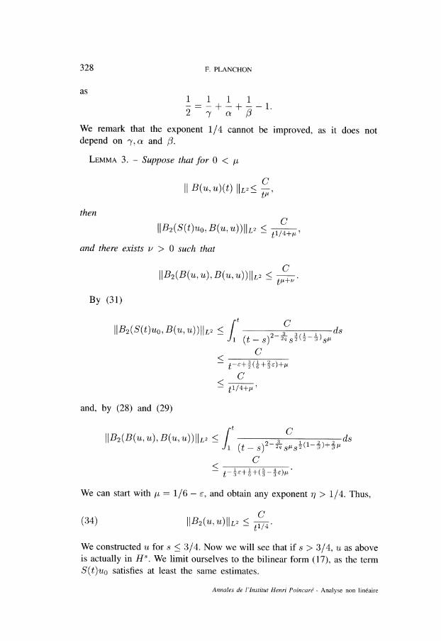
328 F. PLANCHON

as

We remark that the exponent 1 /4 cannot be improved, as it does not

depend on and ,~.

LEMMA 3. - Suppose that for 0 p

then

and there exists v > 0 such that

By (31 )

and, by (28) and (29)

We can start with = 1/6 - ~, and obtain any exponent ~ > 1/4. Thus,

We constructed u for s 3/4. Now we will see that if s > 3/4, u as aboveis actually in We limit ourselves to the bilinear form (17), as the termS(t)uo satisfies at least the same estimates.



LEMMA 4. - Let f, g E Hs(If~3), 3~4 s 3/2,

For a proof see the Appendix. Suppose now that s > 3/4, and u is thesolution of Proposition 3 for s = 3/4. Then, if ~ 1 /4, we obtain for t 1

using Lemma 4 and the boundedness of f in H3~4, so that

which gives the continuity at zero. For t > 1, we have by (29)

which allows us to improve (22), for s 3/4

Then

and,

and

then, for all t

Vol. 13, n° 3-1996.

330 F. PLANCHON

We have thus obtained u E H 4 +’~ . By applying the same argument we canreach the value s > 3/2, as

with ~ + 3/2 - s 1. Before dealing with the case s > 3/2, let us brieflyshow (7) . By Sobolev’s injection theorem (see [14]), if s 3/2 then

with 1/p = 1/2 - s/3. If s = 1 + c~, a 1/2, we obtain, for t, 1

For small t, B ( f , g) is bounded and tends to zero as t goes to zero. Nowwe treat the case where s > 3/2, using the following estimateLEMMA 5. - Let f, 9 E Hs (~3), s > 3/2,

For a proof, see the appendix. We will then show

LEMMA 6. - Let s > 3/2, for all t > 0

This can be achieved by successive iterations, starting from the previousestimate for s = 2, and applying Lemma 5. Let us see how it works ateach step. Let ~ 1, we first treat the case t 1.

and as f and g are bounded in L°° and in Hs,

For t > 1,



by using Lemma 4. Then

For t > 1,

and using Lemma 5 we deduce the estimate for from the estimate for s :

This achieves the proof of the existence of u E BC ( [0, -~-oo ) , Hs ) . Now,we observe that, as we have local existence and uniqueness for s > 1 /2(see [4]), our solution is unique by applying this theorem on intervals

covering [0, oo). In the case s = 1/2, it is necessary to establish uniquenessdirectly, (see [4] or [11]). The reader should refer to [11] or [7], in orderto see why a solution of (11) is actually a solution in the classical sense.We can nevertheless make a few remarks. By the same process we use to

gain the regularity s - 3/4, we can establish, independently of s, estimatesin Hr, r > s : for all t > 0, there exists 7r(r) > 0

and is holderian on every interval provided t 1 > to > O.This

provides the regularity in the space variables. As for regularity in time, it

suffices to use the relation, which can be established without knowing (10)

and the following lemma, (see [ 11 ] or [7] for a proof).

LEMMA 7. - Let = ~o e ~t s~° f (s)ds, t E ~0, T], f E C’~([o, T], B),r~ 1; B a Banach space. Then u E Au E

and

for all v r~.We then obtain the C°° regularity of u, for t > 0, with a bootstrap

argument. Let us see how condition (13) can be expressed on Uo in terms

Vol. 13, nO 3-1996.

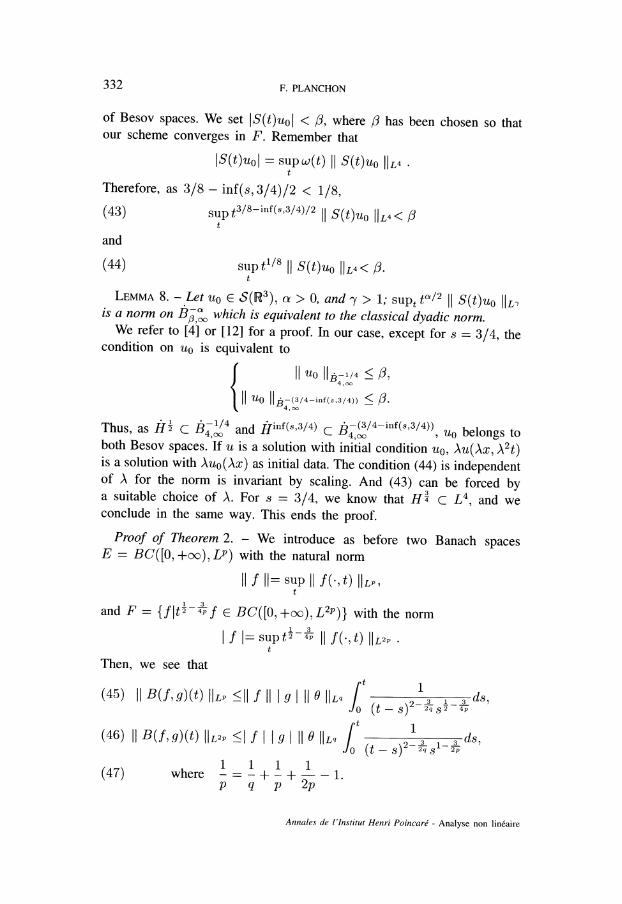
332 F. PLANCHON

of Besov spaces. We set ~3, where ~3 has been chosen so thatour scheme converges in F. Remember that

Therefore, as 3/8 - inf(s, 3/4)/2 1/8,

and

LEMMA 8. - Let uo E S(R3), a > 0, and 03B3 > 1; supt S(t)uo is a norm on which is equivalent to the classical dyadic norm.We refer to [4] or [12] for a proof. In our case, except for s = 3/4, the

condition on uo is equivalent to

Thus, as H 2 C B4, ~4 and C $4 (~/4-inf(s,3/4)) ~ uo belongs toboth Besov spaces. If u is a solution with initial condition uo, À2t)is a solution with as initial data. The condition (44) is independentof A for the norm is invariant by scaling. And (43) can be forced bya suitable choice of A. For s = 3/4, we know that H 4 C L4, and weconclude in the same way. This ends the proof.

Proof of Theorem 2. - We introduce as before two Banach spacesE = BC([O, +(0), LP) with the natural norm

and F vith the norm

then, we see that

where -j


333NAVIER-STOKES EQUATIONS IN ~3

which gives the continuity of B from F x F ~ F and F x E 2014~ E, withconstants and

and a simple rescaling shows both quantities are bounded. Then if we usethe same sequence as before, Lemma 1 gives us the convergence in F, andwe obtain the convergence in E by acontraction argument, as r~(p) we obtain 1. The continuity at t = 0 comes from a slightmodification of (45), as we can replace I f by f ( . , which tends to zero with t. Actually, the value of could

only be zero: the first term ui = S(t)uo tends to zero, for if we consider asequence of Co functions ( v~ ) ~ which approximate uo,

By Lemma 8 the condition on uo becomes,

where 03B4(p) ~ 1/03B3(p). This proves 3Proposition 1. Proposition 2 results

from the inclusion of L3 in B-(1-3 2p)2p,~. Note that for p = 2, we imposethe condition

which is equivalent to the condition (2). For a general uo E L2, we onlyknow

In other words, we do not know enough on low frequencies, and a sufficientcondition is (2), of which uo E L3 or uo E H 2 with small norms areparticular cases. We obtained existence and uniqueness in a ball of F withLemma 1 and uniqueness in the whole space can be obtained directly asin [11] or [4]. As in the Sobolev case, it is possible to obtain estimates onLq norms of ~c( ~, t), q > p, in order to show the C°° regularity for t > 0.

Vol. 13, n° 3-1996.

334 F. PLANCHON

APPENDIX

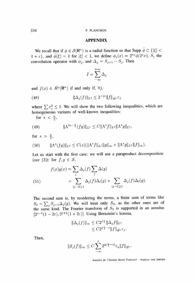
We recall that if rP E S(Rn) is a radial function so that Supp ~ {|03BE| 1 -f- ~~, and ~(~) = 1 for 1, we define the

convolution operator with and Aj = Sj. Then

and f(x) E if and only if, Vj,

where £ ~~ 1. We will show the two following inequalities, which arehomogeneous variants of well-known inequalities:

for s n , 2

for s > 2 ,

Let us start with the first case: we will use a paraproduct decomposition(see [3]): for f, 9 E S,

The second sum is, by reordering the terms, a finite sum of terms like

S2 = ~~ We will treat only S2, . as the other ones are of

the same kind. The Fourier transform of S2 is supported in an annulus

(2~-1 (1 - 2~), 2~+1 (1 + 2~)~. Using Bernstein’s lemma,

Then,



and

is a convolution product between ll and l2, therefore in l2. For j > 0,

if

is in l2 for the same reason as ~~ . This gives

where E l ~ . Then, if is associated to g,

and as E ll C lz, ,Sl E The terms of the first sum in (51)are like 51 = ~~ and in this case we only know that the

support of the Fourier transform of is in {~~~ C2~}, and

LEMMA 9. - If u C L1, supp ic C 1-~ 2s, then

This comes from

then, applying Lemma 9 to

As E this ends the proof. The second inequality can be provedby the same estimates, except that we have a better estimate for ~~,5’~(f)~~~and both bounded by

Vol. 13, n° 3-1996.

336 F. PLANCHON

REFERENCES

[1] H. BEIRÃ O DA VEGA, Existence and Asymptotic Behaviour for Strong Solutions of theNavier-Stokes Equations in the Whole Space, Indiana Univ. Math. Journal, Vol. 36(1),1987, pp. 149-166.

[2] J. BERGH and J. LÖFSTROM, Interpolation Spaces, An Introduction, Springer-Verlag, 1976.[3] J. M. BONY, Calcul symbolique et propagation des singularités dans les équations aux

dérivées partielles non linéaires, Ann. Sci. Ecole Norm. Sup., Vol. 14, 1981, pp. 209-246.[4] M. CANNONE, Ondelettes, Paraproduits et Navier-Stokes, PhD thesis, Université Paris IX,

CEREMADE F-75775 PARIS CEDEX, 1994, to be published by Diderot Editeurs(1995).

[5] J.-Y. CHEMIN, Remarques sur l’existence globale pour le système de Navier-Stokes

incompressible, SIAM Journal Math. Anal., Vol. 23, 1992, pp. 20-28.[6] Y. GIGA, Solutions for Semi-Linear Parabolic Equations in Lp and Regularity of Weak

Solutions of the Navier-Stokes System, Journal of differential equations, Vol. 61, 1986,pp. 186-212.

[7] Y. GIGA and T. MIYAKAWA, Solutions in Lr of the Navier-Stokes Initial Value Problem,Arch. Rat. Mech. Anal., Vol. 89, 1985, pp. 267-281.

[8] R. KAJIKIYA and T. MIYAKAWA, On L2 Decay of Weak Solutions of the Navier-StokesEquations in Rn, Math. Zeit., Vol. 192, 1986, pp. 135-148.

[9] T. KATO, Strong Lp Solutions of the Navier-Stokes Equations in Rm with Applicationsto Weak Solutions, Math. Zeit., Vol. 187, 1984, pp. 471-480.

[10] T. KATO and H. FUJITA, On the non-stationnary Navier-Stokes system, Rend. Sem. Math.Univ. Padova, Vol. 32, 1962, pp. 243-260.

[11] T. KATO and H. FUJITA, On the Navier-Stokes Initial Value Problem I, Arch. Rat. Mech.Anal., Vol. 16, 1964, pp. 269-315.

[12] J. PEETRE, New thoughts on Besov Spaces, Duke Univ. Math. Series, Duke University,Durham, 1976.

[13] J. SERRIN, On the Interior Regularity of Weak Solutions of the Navier-Stokes Equations,Arch. Rat. Mech. Anal., Vol. 9, 1962, pp. 187-195.

[14] E. M. STEIN, Singular Integral and Differentiability Properties of Functions, PrincetonUniversity Press, 1970.

[15] M. TAYLOR, Analysis on Morrey Spaces and Applications to Navier-Stokes and OtherEvolution Equations, Comm. in PDE, Vol. 17, 1992, pp. 1407-1456.

[16] H. TRIEBEL, Theory of Function Spaces, volume 78 of Monographs in Mathematics,Birkhauser, 1983.

(Manuscript received October 24, 1994.)


Documents

Global strong solutions in Sobolev or Lebesgue spaces to the ...archive.numdam.org/article/AIHPC_1996__13_3_319_0.pdf · Global strong solutions in Sobolev or Lebesgue spaces to the