Global Solar Radiation Estimation and Calculating the

Advances in Dynamical Systems and Applications (ADSA).

ISSN 0973-5321, Volume 16, Number 2, (2021) pp. 881-894

© Research India Publications

https://www.ripublication.com/adsa.htm

Global Solar Radiation Estimation and Calculating

the Corresponding Regression Coefficients

for Bangalore

Mr. Madhu MC1*, Mr. A. Hemanth Kumar2, Mr. Pramod Manjunath3,

Mr. K. Badari Narayana4, Mr. H. Naganagouda5

1*Assistant Professor, Department of Mechanical Engineering, BMS Institute of Technology and Management, Avalahalli, Yelahanka, Bangalore, Karnataka, India.

2Research Assistant, Department of Mechanical Engineering, BMS Institute of

Technology and Management, Bangalore, India. 3Research Assistant, Department of Mechanical Engineering, BMS Institute of

Technology and Management, Bangalore, India. 4Principal Consultant, COE Aerospace & Defence, Visvesvaraya Technological

University, Nagarabhavi, Bangalore, India. 5Former Director, Centre for Solar Technology, KPCL, Bangalore, India.

Abstract

This paper investigates the solar potential for Bangalore using the global

horizontal irradiance, measured for a period of four years (January 2014 to

November 2018). The consistency of the collected data is further analysed,

and the relative sunshine hours is established. From the available sunshine

hours, the data is analysed for daily, monthly, seasonal and annual average and

annual peak values. The results of the various average values are computed

from the measured data and the theoretically estimated data are compared for

Bangalore region. Furthermore, a regression analysis is performed using

measured and theoretical data, a theoretical model based on linear fit for a

better prediction of global solar radiation for Bangalore region is developed.

The main objective of this paper is to present the regression coefficients of a

linear model a & b which is found out to be 0.27 and 0.62 for 2015, 0.3 and

0.53 for 2016 and 0.18 and 0.67 for 2017, which have been calculated for

Bangalore city. The coefficients estimated from the current model are very

closely matching with those mentioned in the literature for Bangalore.

Keywords: Global solar radiation, Annual average, Seasonal average,

Regression Coefficients a & b, India.

882 Mr. Madhu MC et al.

NOMENCLATURE:

H Measured Global Solar Radiation (W/m2)

�̅� Measured Monthly Average of Global Solar Radiation (W/m2)

H0 Estimated Global Solar Radiation (W/m2)

�̅�0 Estimated Monthly Average Global Solar Radiation (W/m2)

N Sunlight Hours (hours)

�̅� Monthly average of maximum possible Sunlight hours (hours)

n Day number of year

�̅� Experimental Sunshine hour

a, b Regression/Angstrom Constants

Isc 1367 Wm-2 (Solar Radiation Constant)

Ø Latitude of the location (°)

δ Declination of the angle (°)

ω Sunset Hour angle (°)

r Correlation Coefficient

SR Solar Radiation

1. INTRODUCTION

The Sun’s energy is the main and primary source of energy which drives the Earth’s

atmosphere and oceans. The energy in the form of radiation moves through empty

space from the Sun to the Earth and drives and controls the weather, climate and more

importantly life. Virtually all the exchange of energy in the universe takes place by

radiation. This radiation is in the form of electromagnetic wave, emitted by the Sun

throughout the solar system Enters the Earth’s atmosphere. The total radiation

reaching the surface of the Earth is known as the Global Radiation. This Global

Radiation is a combination of beam radiation, diffused radiation and reflected

radiation (Also known as the Earths Albedo Effect).

In order to choose the right solar power setup for a specific geographic location, one

may want to measure and understand the amount of solar energy that falls on the

surface around that area. Given the global radiation of the place, an accurate

Global Solar Radiation Estimation and Calculating the Corresponding… 883

estimation can be calculated to estimate the global radiation for future purpose. This

information is used in design, development and to create accurate estimation models

of solar system performances which constitute an integral input for any solar energy

project. The objective of this study is to develop a correlation between solar radiation

and sunlight hours for a complete span of one year. This study is then extended to

four years. The obtained values of the coefficients are used for creating a stand-alone

power system being tried out in Bangalore.[1]

2. OBJECTIVESOF CURRENT WORK:

To processthe measured data obtainedfrom pyranometer during the years 2015 –

2018

To estimate average and peak solar radiation and understand their trends

To find global and average solar radiation by applying available theoretical &

analytical solutions[2]

To calculate the regression coefficients a and b from the measured values.

The solar radiation data is obtainedfrom the solar laboratory located in the

Department of Physics at BMSCE, Bangalore, where pyranometers are used to

measure the radiation. The data obtained is grouped and then the data set is ready to

be analysed. Here it has been analysed in the form of pivot tables and charts depicting

the result of the data from the year 2015 to 2018. The average and peak values are

found out and displayed in the form of tables and relative graphs plotted to study their

trends.

The average values, the number of sunlight hours &number of days of global

radiation of a data set (Monthly and seasonally) are used to compute the average solar

radiation assuming normal conditions. Regression Analysis was performed on the

data by using relevant analytical expressions

3. MEASUREMENTS AND MATHEMATICAL MODEL:

The suitable instrument to measure the global radiation which includes diffused

radiation obtained from a Pyranometer. The product used for this study is a “LI-

200SA Pyranometer Sensor” available at the Physics laboratory at BMS College of

Engineering, Bengaluru (Altitude: 920m from Sea level). This instrument measures

the radiation incident on horizontal surface. The spectral range covers wavelengths

from 0.4µm to 1.2µm[3].This instrument also measures the temperature data in degree

Celsius (°C). The following parameters are measured by the pyranometer and

imported to Microsoft Excel in the following format;

a. Date: [DD-MM-YYYY HH:mm]

b. Temperature: [°C]

c. Solar Radiation: [SR, W/m2]


Measurements are made for every hour of the day from the 1stJanuary 2015 to 15th

November, 2018. This instrument is also capable of measuring other parameters such

as α rays, ß rays, etc.[Refer Appendix A]. A sample measured data is as measured

data is shown in Table A1.

3.1 Analysis of Measured Data:

1.The data is processed in Microsoft excel by filtering them and keeping only the

sunshine hours data which is from 6am to 4pm. Furthermore “Power Off” data

was filtered out [Refer Appendix B]. Details of different sources of data

deficiencies asdiscussed, are carefully filtered out.

2.The data for four years was combined, and a pivot chart and table were created.

3.From the analysis of pivot table, various parameters were found out such as;

Monthly Peak Solar Radiationand Peak Temperature during sunshine hours

Monthly Average Solar Radiation

Seasonal Average (Winter, Summer, Spring and Autumn)

4.Estimating of monthly global radiation to find the regression constants a&b.

3.2 Mathematical Model:

The mathematical model for comparing the measured radiation values and calculated

radiation values followed here arewith reference to Debazit Datta, et al.[4], Sekar, et

al.[5],Salima, et al.[6] and Gungor et al.[7]. From the literature, the error statistics

usedwere MAPE, MBE,and RMSE. Linear fit, quadratic fit and exponential fit were

used generally. For the present work. a Linear fit is considered, which serves as the

simplest and most suitable method as observed from literature.

A. Çağlar, C. Yamali et al. [8] showed that the liner and quadratic models gave the

least errors for the monthly estimated values. The estimated values were very similar

to the linear model using the logarithmic and exponential regression values. Since the

differences are extremely small and for simplicity the liner model is widely accepted

and practised to estimate the global solar radiation.

The linear equation is the best overall and has the best performance since the

difference between the various models are negligible and also, it is easy to understand

the linear equations. The estimation done in this paper uses the linear model to

estimate the average monthly global solar radiation for Bangalore location, and the

same can be used in the initial design of solar power requirements for both residential

and major solar parks. The difference in the values between the actual measurements

of the solar radiation and the solar radiant energy estimated by proposed equations

show a nearly normal distribution compared with other models [9]. The low error

between the measured and the estimated value makes this, linear model a reliable

tool.[10]


This study uses the liner model proposed by Angstrom for estimating the total solar

radiation in Bangalore. The data collected were for a period of four years from 2015

to 2018. The data points were the global horizontal irradiance and the temperature at

every 1hr interval.[11]

3.2.1 Sample Calculation In this below calculation we estimate the mean monthly solar radiation.

The average sunlight hours being considered for this study is;

N = 10 hours

The day numbers;

n = 1st day

Latitude of Bangalore,

Ø = 12.97°

The solar constant “Isc” is as follows;

Isc = 1367 W/m2

“δ”, declination angle is given by;

δ = 23.45 sin (360[𝑛+284]

365) = 23.45 sin (

360[1+284]

365) = -23.38°

The sunrise hour angle“ω” is given by; [12]

ω = cos-1∗ (− tan(Ø) tan(δ)) = cos-1∗ (− tan(12.98°) tan(−23.38 °)) = 84.28°

Maximum sunshine Hours possible for a given day is:

N = ω∗2

15 = 84.28°∗

2

15= 11.23 hours

Hence with all the parameters being found out, the average monthly global solar

radiation is found out;

H0 = 𝐼𝑠𝑐

𝜋[1 + 0.033 ∗ cos(

360 𝑛

365)] [cos(∅) cos(𝛿) sin(𝜔) +

𝜋𝜔

180sin(∅) sin(𝛿)]

= 350.32 W/m2[4]


After finding out the mean monthly global solar radiation, the mean values of H & H0

and n and N are calculated. Their corresponding ratios are found out for further

analysis

Table 1: Ratio of Measured and Theoretical values for 2015

From Table 1, it is evident the extra-terrestrial H0 avgis higher than the measured

average monthly solar radiation. The clearness index H/H0 is always less than one.

4. RESULTS

In this section, the results of peak solar radiation are shown in Fig1 and 2 and data is

shown in Table1,.While the average monthly global radiation is shown in Fig3 and

the seasonal average global solar radiation is depicted by Fig 4,5,6 and 8. Also, the

computational results of comparison between estimated and measured solar radiation

which leads to finding the regression coefficients “a &b” are discussed.

Month H avg Navg H0avg Navg Havg/H0

avg

n avg/

Navg

Jan 297.00 11.00 352.81 11.32 0.84 0.97

Feb 374.00 11.00 388.07 11.60 0.96 0.95

Mar 373.00 12.00 421.00 11.93 0.89 1.01

Apr 352.00 12.00 440.58 12.30 0.80 0.98

May 338.00 12.00 441.75 12.61 0.77 0.95

Jun 300.00 9.81 437.64 12.76 0.69 0.77

Jul 282.00 7.01 437.91 12.69 0.64 0.55

Aug 278.00 11.00 438.22 12.42 0.63 0.89

Sep 303.00 10.21 425.13 12.06 0.71 0.85

Oct 330.00 10.32 394.78 11.69 0.84 0.88

Nov 204.00 11.00 358.69 11.38 0.57 0.97

Dec 271.00 11.00 340.85 11.24 0.80 0.98


4.1 Peak Global Solar Radiation:

Figure. 1 shows the peak global solar radiation on a given day for the years 2015 to

2018 (November). It can be noted here that the peaks are attained during the post

monsoon seasons of August and September which pertains to the unusual trend that

can be noticed only here in Bangalore.

Figure 1: Monthly Peak Solar Radiation (2015 - 2018)

Figure. 2 shows the peak Solar Radiation and the corresponding to the peak temperature variations for every month over four years. Since solar radiation and the

corresponding factors that influence of radiation yield are important data for

designing an efficiently photovoltaic devices, a glimpse of that can be observed from

these distributions. The sun’s radiation reaching the earth’s surface has different

values during the day.Factors such as cloud cover, wind-velocity, humidity, sky

clearness index, etc. have great affect the solar radiation incident on the surface.

Neglecting the dependence of these factors,apart from the general variation in

temperature and solar radiation that can be observed, the radiation is different for

similar temperature values on different days.

From Figure 2 we can observe that with increase in temperature the amount of Solar

Radiation being harnessed is considerably low when compared with the points where

the Solar Radiation is higher with a lower temperature. [15]


Figure 2: Monthly Peak Solar Radiation (2015 - 2018)

4.2 Average Monthly Global Solar Radiation:

The average monthly global solar radiation is the average of solar radiation(as shown

in Figure3)incident for that month. As the onset of summer approaches, the average

values are highest in the February, March, April and May. From this trend, it can also

be observed that the Sun is traversing to the Southern hemisphere from the Northern

hemisphere. [16]

Figure3: Monthly Average Solar Radiation (2015 - 2018)


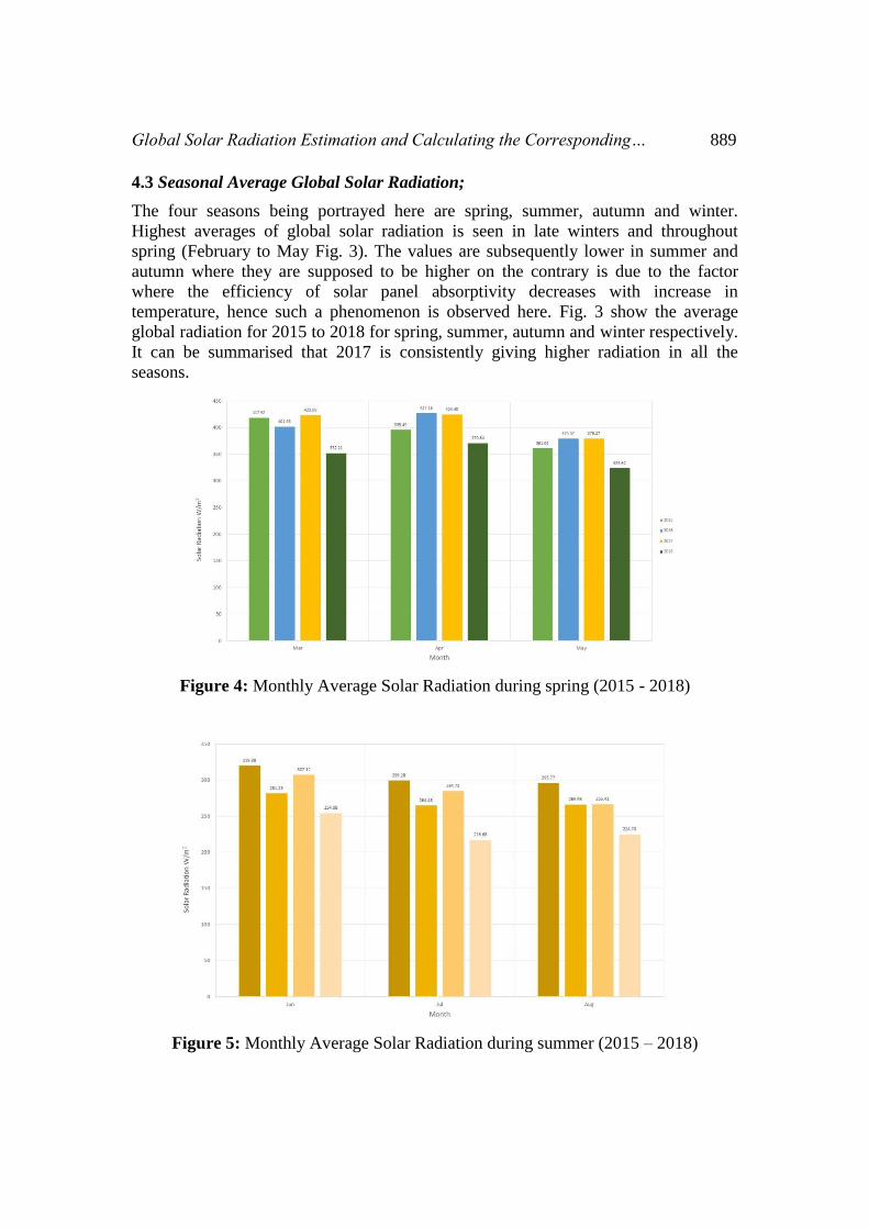
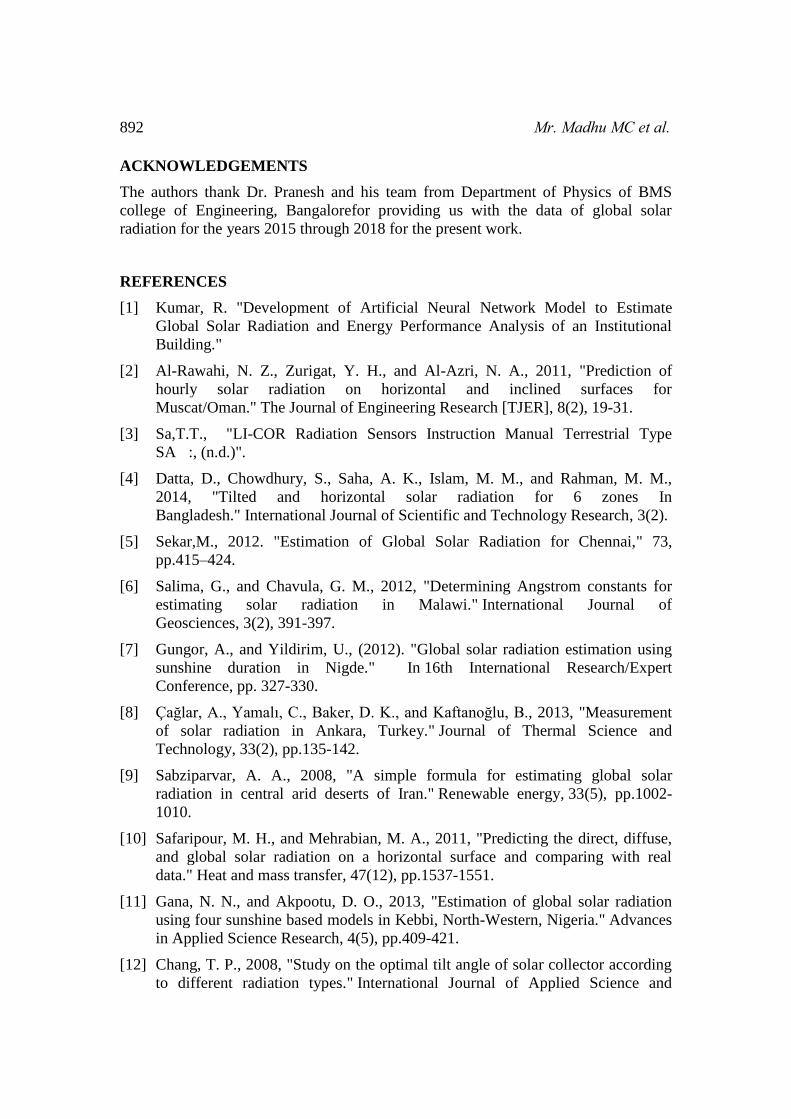
4.3 Seasonal Average Global Solar Radiation;

The four seasons being portrayed here are spring, summer, autumn and winter.

Highest averages of global solar radiation is seen in late winters and throughout

spring (February to May Fig. 3). The values are subsequently lower in summer and

autumn where they are supposed to be higher on the contrary is due to the factor

where the efficiency of solar panel absorptivity decreases with increase in

temperature, hence such a phenomenon is observed here. Fig. 3 show the average

global radiation for 2015 to 2018 for spring, summer, autumn and winter respectively.

It can be summarised that 2017 is consistently giving higher radiation in all the

seasons.

Figure 4: Monthly Average Solar Radiation during spring (2015 - 2018)

Figure 5: Monthly Average Solar Radiation during summer (2015 – 2018)


Figure 6: Monthly Average Solar Radiation during autumn (2015 – 2018)

Figure 7: Monthly Average Solar Radiation during winter (2015 – 2018)

5. COMPARISON AND DISCUSSIONS:

The calculated values of solar radiations were then compared to measured data for

each year, shows that both models are consistent with the observed/measured data. As

the Sun’s energy in the form of radiation enters the Earth’s atmosphere, the radiation

is experiences scattering and absorption due to the presence of moisture, dust, gases,

clouds and other particles present in the atmosphere, and some of the radiation is

reflected back to the space. Thus, the total solar radiation incident of the Earth’s

surface is always less than the extra-terrestrial radiation H0.[17]


Through a scattered plot the findings of the correlation coefficient are illustrated. The

figure 8 depicts the graph plotted between �̅�/�̅�0and �̅�/�̅�. From the slope of the graph

we obtain the values of constants of the linear equationa & b. The Rvalues shows the

accuracy of the computed data and to which extent the values are closer to mean line.

Figure 8: 2015 Correlation Coefficient and Regression Constant

6. CONCLUSION

The measured value it was confirmed that the total solar radiation increases from

February to April and August to October. The linear model has been used to estimate

the regression coefficients of Bangalore. The coefficients of regression, i.e. a and b

were established as 0.27and 0.62respectively for 2015, 0.3 & 0.53 respectively for

2016 and 0.18 & 0.67 respectively for 2017 which averages to 0.25 & 0.61, whereas

according to widely accepted reference values for the same location are 0.18 and 0.64

for a & b respectively.

Hence the regression coefficients are well within the acceptable range of deviation

and the latest value available for this region which has been optimised particularly for

Bangalore.

The climatic conditions and the local weather conditions vary every year, but the

values shown in the results in this study based on four years of observed data would

be best recommended to engineers. Since no research regarding regression

coefficients has been done prior to this work in the recent years, this study will be

very helpful to use this information for Bangalore.

Using this data, it is possible to find out the close relation to measured and theoretical

values which in turn can be used to find out the optimal orientation of solar panel for

maximum yield of solar radiation. [18]

The effort to estimate solar radiation from measured meteorological parameters in

Bangalore will contribute to the development of a fine-tuned model in the upcoming

years.


ACKNOWLEDGEMENTS

The authors thank Dr. Pranesh and his team from Department of Physics of BMS

college of Engineering, Bangalorefor providing us with the data of global solar

radiation for the years 2015 through 2018 for the present work.

REFERENCES

[1] Kumar, R. "Development of Artificial Neural Network Model to Estimate

Global Solar Radiation and Energy Performance Analysis of an Institutional

Building."

[2] Al-Rawahi, N. Z., Zurigat, Y. H., and Al-Azri, N. A., 2011, "Prediction of

hourly solar radiation on horizontal and inclined surfaces for

Muscat/Oman." The Journal of Engineering Research [TJER], 8(2), 19-31.

[3] Sa,T.T., "LI-COR Radiation Sensors Instruction Manual Terrestrial Type

SA  :, (n.d.)".

[4] Datta, D., Chowdhury, S., Saha, A. K., Islam, M. M., and Rahman, M. M.,

2014, "Tilted and horizontal solar radiation for 6 zones In

Bangladesh." International Journal of Scientific and Technology Research, 3(2).

[5] Sekar,M., 2012. "Estimation of Global Solar Radiation for Chennai," 73,

pp.415–424.

[6] Salima, G., and Chavula, G. M., 2012, "Determining Angstrom constants for

estimating solar radiation in Malawi." International Journal of

Geosciences, 3(2), 391-397.

[7] Gungor, A., and Yildirim, U., (2012). "Global solar radiation estimation using

sunshine duration in Nigde." In 16th International Research/Expert

Conference, pp. 327-330.

[8] Çağlar, A., Yamalı, C., Baker, D. K., and Kaftanoğlu, B., 2013, "Measurement

of solar radiation in Ankara, Turkey." Journal of Thermal Science and

Technology, 33(2), pp.135-142.

[9] Sabziparvar, A. A., 2008, "A simple formula for estimating global solar

radiation in central arid deserts of Iran." Renewable energy, 33(5), pp.1002-

1010.

[10] Safaripour, M. H., and Mehrabian, M. A., 2011, "Predicting the direct, diffuse,

and global solar radiation on a horizontal surface and comparing with real

data." Heat and mass transfer, 47(12), pp.1537-1551.

[11] Gana, N. N., and Akpootu, D. O., 2013, "Estimation of global solar radiation

using four sunshine based models in Kebbi, North-Western, Nigeria." Advances

in Applied Science Research, 4(5), pp.409-421.

[12] Chang, T. P., 2008, "Study on the optimal tilt angle of solar collector according

to different radiation types." International Journal of Applied Science and


Engineering, 6(2), pp.151-161.

[13] Loutzenhiser, P. G., Manz, H., Felsmann, C., Strachan, P. A., Frank, T., and

Maxwell, G. M., 2007, "Empirical validation of models to compute solar

irradiance on inclined surfaces for building energy simulation." Solar

Energy, 81(2), pp.254-267.

[14] Jamil, B., Siddiqui, A. T., and Akhtar, N., 2016, "Estimation of solar radiation

and optimum tilt angles for south-facing surfaces in Humid Subtropical Climatic

Region of India", Engineering Science and Technology, an International

Journal, 19(4), pp.1826-1835.

[15] Bajpai, U., and Singh, K., 2009, "Estimation of instant solar radiation by using

of instant temperature." ActaMontanisticaSlovaca, 14(2), pp.189.

[16] El Mghouchi, Y., El Bouardi, A., Choulli, Z., and Ajzoul, T. 2014, "New model

to estimate and evaluate the solar radiation." International Journal of

Sustainable Built Environment, 3(2), pp.225-234.

[17] Dlamini, M. D., Varkey, A. J., and Mkhonta, S., 2017, "Models for calculating

monthly average solar radiation from air temperature in Swaziland."

[18] Li, D. H., and Lam, T. N., 2007, "Determining the optimum tilt angle and

orientation for solar energy collection based on measured solar radiance

data." International Journal of Photoenergy, 2007.

APPENDIX A: Sample measured data

Table A1 shows the sample data collected from the pyranometer.

Table A1: Sample of Data

Date Temp. ˚C SR W/m²

01-01-2015 08:00 Power off Power off





01-01-2015 13:00 27.6 552

01-01-2015 14:00 27.8 433

01-01-2015 15:00 28.2 367

01-01-2015 16:00 27.6 147

01-01-2015 17:00 26.9 41

01-01-2015 18:00 26.0 7

01-01-2015 19:00 25.4 7

01-01-2015 20:00 25.1 7


APPENDIX B: Different sources of deficiencies in the measured data

The data obtained has discrepancies in short duration in the form of missingvalues

which is inevitable due to power failure or malfunctioning of instrument. Faulty

readings such as positive values of solar irradiation after sunset which is not possible

(also part of the data discrepancy) and can be attributed to light pollution from the city

streetlights&reflected light from buildings about the same time.The instrument had

been powered off due to maintenance purpose. All the above condition may resultin

displaying “Power Off’ values. However, these faulty data do not affect the present

study since they are being filtered out. A sample of the filtered values used in the

current work is given in Table B1.

Table B1: Filtered Data

Date Temp. ˚C SR W/m²

01-01-2015 13:00 27.6 552

01-01-2015 14:00 27.8 433

01-01-2015 15:00 28.2 367

01-01-2015 16:00 27.6 147

02-01-2015 06:00 22.6 7

02-01-2015 07:00 22.8 58

02-01-2015 08:00 24.1 123

02-01-2015 09:00 24.9 247

02-01-2015 10:00 25.2 254

02-01-2015 11:00 26.0 339

02-01-2015 12:00 26.8 421

Documents

Global Solar Radiation Estimation and Calculating the