Global localization for mobile robots using reference scan matching

International Journal of Control, Automation, and Systems (2014) 12(1):156-168 DOI 10.1007/s12555-012-9223-0

ISSN:1598-6446 eISSN:2005-4092http://www.springer.com/12555

Global Localization for Mobile Robots using Reference Scan Matching

Soonyong Park and Sung-Kee Park*

Abstract: This paper presents a new approach based on scan matching for global localization with a metric-topological hybrid world model. The proposed method aims to estimate relative pose to the most likely reference site by matching an input scan with reference scans, in which topological nodes are used as reference sites for pose hypotheses. In order to perform scan matching we apply the spec-tral scan matching (SSM) method that utilizes pairwise geometric relationships (PGR) formed by fully interconnected scan points. The SSM method allows the robot to achieve scan matching without using an initial alignment between two scans and geometric features such as corners, curves, or lines. The lo-calization process is composed of two stages: coarse localization and fine localization. Coarse localiza-tion with 2D geometric histogram constructed from the PGR is fast, but not precise sufficiently. On the other hand, fine localization using the SSM method is comparatively slow, but more accurate. This coarse-to-fine framework reduces the computational cost, and makes the localization process reliable. The feasibility of the proposed methods is demonstrated by results of simulations and experiments. Keywords: Global localization, hybrid map, mobile robot, pairwise geometric relationships, scan matching.

1. INTRODUCTION

Mobile robot localization is the problem of estimating

a robot’s pose relative to its environment [1], in which it is assumed that the robot is provided with a map of the environment [2]. The localization problem can be classi-fied into two cases: local pose tracking and global locali-zation. Given its initial pose, local pose tracking tries to keep track of the robot’s pose as the robot moves. Global localization aims to estimate the robot’s pose using only the current sensor data without knowing a priori pose information, which provides mobile robots with abilities to deal with initialization at startup and recovery from pose tracking failure.

Many localization methods have been studied so far; these methods make use of different sensors including range finders [1,3,4] or cameras for vision [5-7]. These methods also use various algorithms and techniques [4]. The general approach to address the localization problem is to compare information extracted from sensor readings

with a previously learned map [8]. The comparison is typically carried out by measuring the similarities bet-ween the sensing data and the reference data which are computed from pose hypotheses on the map. Each similarity embodies some evidence about where the robot might be located. Accordingly, the goal of locali-zation is, as efficiently as possible, to detect the most likely hypothesis and to estimate the correct pose with respect to some reference frame; at this point, the performance of localization depends on three factors: 1) the type of map to be used for localization, 2) the manner to select pose hypotheses, and 3) the method to measure the similarity.

One possible way to achieve the localization is to use range scan matching, which is to estimate the relative pose between two successive locations by maximizing the overlap between an input scan and a reference scan obtained at each location. On account of its high reliability and accuracy, scan matching has been widely employed to many localization algorithms [9-15]. Most of the scan matching methods use an initial alignment between two scans, which is typically given from dead reckoning data [16-18]. This kind of scan matching methods is appropriate for local pose tracking; however, these methods cannot be used for global localization, in which the robot estimates its pose without initial pose information. Other scan matching methods using geometric features such as corners, curves, or lines are applicable to global localization [9,19-23]. Although this type of method does not need an initial alignment, it cannot be used in unstructured environments where such geometric features are hardly extracted. From this view-point, in order to realize global localization based on scan matching, it is desirable to apply a scan matching method without using an initial alignment and geometric

© ICROS, KIEE and Springer 2014

__________

Manuscript received May 24, 2012; revised December 13,2012 and July 25, 2013; accepted October 23, 2013. Recommend-ed by Associate Editor Seul Jung under the direction of EditorHyouk Ryeol Choi. This work was supported by the KIST Institutional Program(2E24123) and the NAP (National Agenda Project) of the KoreaResearch Council of Fundamental Science & Technology. Soonyong Park is with the Global Technology Center, Sam-sung Electronics, Maetan 3-dong, Yeongtong-gu, Suwon-si,Gyeonggi-do 443-803, Korea (e-mail: [email protected]). Sung-Kee Park is with the Center for Bionics/Biomedical Re-search Institute, Korea Institute of Science and Technology(KIST), Hwarangno 14-gil 5, Seongbuk-gu, Seoul 136-791, Korea(e-mail: [email protected]). * Corresponding author.


157

features. In this paper, we propose a scan matching-based

approach for global localization based on a metric-topo-logical hybrid map. As a core concept for overcoming the previous drawbacks such as initial alignment and geometric feature extraction, we introduce our spectral scan matching (SSM) method developed in [24] as a part of this paper, which uses only geometric parameters of interconnected scan points as seen in Fig. 1. However, because the SSM method becomes slow in proportion to the size of environmental map, we also suggest a coarse-to-fine global localization strategy for reducing the time complexity. In coarse localization, by 2D geometric histogram-based template matching, we select a few candidate sites where the robot may be near. Then, the SSM method is used for determining the correct site among the candidate sites and estimating the relative pose with respect to the correct site. Our method can be also used for both structured and unstructured environ-ments, and is applicable even if unknown dynamic objects exist or the scan data are partially corrupted because it uses the whole scan points instead of a few extracted features, which will be shown in Section 6 of this paper.

The rest of this paper is organized as follows. Section 2 addresses related works. Section 3 introduces the SSM method. Section 4 presents how we build reference sites and extract reference scans from a metric-topological map. In Section 5, we describe the coarse-to-fine frame-work for global localization. Experimental verifications are shown in Section 6 and some concluding remarks are given in Section 7.

2. RELATED WORK

2.1. Scan matching

One of the major differences between the existing scan matching algorithms is the usage, or not, of an initial alignment (rotation and translation) between two scans. As described in [9], the scan matching methods can be classified into two types: sequential matching and global matching.

The sequential scan matching compares two succes-sive scans with an initial assumption of alignment between them, in which the initial value is typically obtained by dead reckoning in advance. In a manner of iterative search beginning at the initial alignment, it finds an optimal alignment so that the matching errors between two scans are minimized. When a bad initial alignment is given, however, the sequential scan matching might fail to align two scans because the initial value is possible to lead the matching result to a local minimum. The iterative closest point (ICP) method [16], which is a popular algorithm for matching sets of points or free-form curves and surfaces, uses Euclidean distance to evaluate the matching error between two scans. The LM-ICP method [17] uses the Levenberg-Marquardt algorithm, where the matching error is directly minimized using the sum of squares of nonlinear functions. The iterative dual correspondence (IDC)

method [10] solves the matching problem by searching the translation component and the rotation component separately. The stochastic scan matching method [11,18] uses a sampling-based (Monte Carlo) inference tech-nique. This method transforms each scan into a binary grid image to detect correspondences between two scans, and it recursively computes the weight of each sample with the overlap between grid images. This group of methods is applicable to unstructured environments in-cluding arbitrary shapes such as free-form curves.

On the other hand, the global scan matching does not require an initial alignment, but it needs to detect polygonal features such as corners, curves, or lines. Therefore, it is difficult to use the global scan matching in unstructured environments where such features are scarcely detected. The CCF method [19] matches two scans using the normalized cross correlation between angle histograms of the scans as well as x and y histograms. The APR method [20] matches two scans with the pattern of anchor points such as corners or vertical intersections extracted from the scans. The HSM method [21] extracts line segments from a scan using the Hough Transform and matches them with a set of reference line segments in the Hough domain. These methods are hard to be applicable in the case that each scan contains a number of short line segments or curves. The signature-based method [9] extracts Euclidean invariant signatures from a scan, and it uses a geometric hashing scheme to match two scans with their signatures. This method, however, requires that the scan contains curved objects. The curvature-based method [22] matches two scans using the adaptive curvature function which divides the scans into curve segments and line segments. This method needs the process for estimating the curvature function, and it is hard to provide a good result in the case that the scan includes many short arbitrary segments. The FLIRT method [23] encodes the local structure in the scan around detected interest points into distinctive descriptors. It finds the set of corre-sponding interest points by matching the descriptors using a nearest neighbor strategy and RANSAC algorithm. This method needs a process to detect stable interest points, which may not guarantee good results if the scan includes only a few interest points.

2.2. Global localization

A number of global localization methods have been developed so far. We can classify them into two approaches: probabilistic filter-based method and scan matching-based method. The probabilistic filter-based methods estimate a robot’s pose through conditional probabilistic distribution, called belief, that is computed recursively over the state space of mobile robot’s pose. The most general algorithm for calculating the belief distribution is provided by the Bayes filter algorithm [25], which algorithm allows robots to continuously update their most likely pose within a coordinate system, based on the most recently acquired sensor data. There are three methods derived from the Bayes filter algorithm for providing a solution to the global localization problem:

Soonyong Park and Sung-Kee Park

158

multi-hypothesis Kalman filters, grid-based filters, and particle filters. Multi-hypothesis Kalman filters [8,26,27] represent the belief distribution by mixtures of Gaussians, in which each Gaussian corresponds to one pose hypothesis. This group of methods uses a standard Kalman filter-based tracking module in order to independently update each pose hypothesis. However, they rely on a few detected features instead of using the whole sensor data. Grid-based filters [28-30] discretize the environment into fine-grained grids, in which the grids correspond to all possible poses. The belief distribution is represented by a discrete, piecewise constant set of positional probabilities assigned to each grid. These methods can provide accurate pose estimations with high robustness against sensor noise. However, grid-based filters require a lot of memory and computational cost because the complexity increases exponentially according to the number of grids. Particle filters such as Monte Carlo localization [1,4] and CONDENSATION [31,32] represent the belief distribution by a set of samples. These methods can deal with arbitrary distributions as well as Gaussian, and they can reduce the computational complexity because discretization needs not to be done. However, particle filters may fail to keep track of robot pose if the number of samples is not sufficient. These probabilistic filter-based approaches recursively update the belief distribu-tion. Therefore, the robot should move around its environment in order to acquire new sensor data for the update. In the context of moving to a goal position, however, such wandering movement can be a drawback for efficient navigation.

Most of the scan matching-based global localization approaches adopt the global scan matching methods, whereas the sequential scan matching methods are not applicable to global localization because they need an initial alignment. Zhang and Ghosh [13] proposed a method to make use of line segments extracted from a scan, in which the environment is represented as closed line segment (CLS) map. Global localization is to find corresponding line segments in the map, and the relative pose of an input scan in the environment is computed from the corresponding pairs. Grisetti et al. [14] presented a method called Global Hough Localization. They used the Hough Transform to detect line segments from a scan. Global localization is performed by matching the line segments with a map of line segment in the Hough domain. The robot pose is represented as a set of Gaussians. Tomono [9] applied the signature-based scan matching method to global localization. This approach generates invariant signatures of an input scan, and finds the candidate alignments between the input scan and a set of reference scans using the signatures. Robot pose is determined as the candidate having the best matching score. Weber et al. [15] proposed a hybrid method for global localization. The APR method provides for an input scan several possible alignments within a set of reference scans. The resulting multiple pose hypotheses are tracked and evaluated by a Bayesian tracking technique.

The work described in this paper is a kind of scan matching-based approach, which realizes global localization by matching an input scan with a set of reference scans. A part of this paper was introduced in [12]. The advantage of our localization approach is three folds. First, our method can be used to both grid maps and topological maps having metric information. Second, the use of spectral scan matching method allows our approach to be applicable to both polygonal environ-ments and unstructured environments. Third, our method enables the robot to estimate its pose without roaming motion since the SSM method does not need an initial alignment between two scans.

3. SPECTRAL SCAN MATCHING

Our spectral scan matching (SSM) method consists of

two stages. First, a spectral technique [33] is used to find geometrically consistent correspondences by using pairwise geometric relationships between scan points. And second, a RANSAC-based estimation method [34] is used to estimate robot pose. The scan considered in this paper is 2D raw data measured on horizontal plane.

3.1. Pairwise geometric relationships

We suppose the robot starts at location Rref and acquires a scan Sref. The robot then moves to a new location Rnew and takes another scan Snew. Let

refS =

1{ , , }

n…p p and

1{ , , }

new mS = …r r be the sets of scan

points acquired in each given location. Let Q be a set of correspondence pairs ( , ),i i′ where

refi S∈ and i′∈

Snew. We define the local reference frame of every scan point pi as shown in Fig. 1 (a). The origin is located at the scan point and the x axis is the tangent direction ui, for which we use the approximation:

1 1

1 1

.

i i

i

i i

+ −

+ −

−

=

−

p pu

p p� � (1)

Fig. 1(b) shows the pairwise geometric relationships be-tween two scan points. For a pair of scan points ( , ),i j we compute their distance-angular relationships:

, ( ),ij i j ij i j

arccosρ θ= − = ⋅p p u u� � (2)

where ij

ρ represents the distance between the origin pi and scan point pj, while

ijθ is the angle of the vector

(a) (b)

Fig. 1. (a) Local reference frame of a scan point pi

having tangent direction ui. (b) Pairwise geomet-ric relationships: distance-angular relationships (ρij and θij) between two scan points pi and pj.


159

from the origin pi to scan point pj. We consider the same type of pairwise relationship for the pair of ( , )i j′ ′ which are matched with ( , ).i j We can then define a vector describing the geometric deformations between the scan points ( , )i j and their matched points ( , )i j′ ′ :

2 2( , ) [1 ( ) ( ) ] .Tij ij i j ij i ji j d d θ θ′ ′ ′ ′

′ ′ = − −g (3)

For every pair of possible correspondences ( , )a i i′= and ( , ),b j j′= we define a pairwise potential Gab. This pairwise potential captures the degree to which the two correspondences are compatible geometrically, and it is represented in the form of a logistic function [35]:

( )1

,1 ( ( , ))

ab Tij

Gexp i j

=

′ ′+ −w g

(4)

where ( , )iji j′ ′g is the geometric deformation vector

and w is a regression coefficient vector.

3.2. Detection of consistent correspondences Our matching method is based on a spectral technique

[33], which considers the matching problem as a quadratic assignment problem. It finds the set Q of correspondence pairs ( , )i i′ that maximizes the matching score:

( ) ( ) ( , ) T

a b Q

E a b a b, ∈

= = ,∑ x x G x Gx (5)

where x is binary indicator vector with an element for each correspondence pair ( , )a i i′= such that ( ) 1a =x if scan point i in Sref is matched with i′ in Snew (e.g.,

)a Q∈ and 0 otherwise. Q is a subset of the set L of all tentative correspondences. G is an affinity matrix which consists of pairwise potential: ( , ) .

aba b =G G It is built

symmetrically with every pair of correspondences ,a b∈ L. The diagonal elements of the affinity matrix Gaa is set to 0, and off-diagonal elements are computed by (4). In addition, if the geometric deformation between ( , )i j and ( , )i j′ ′ is too large or if they do not satisfy the mapping constraints (e.g., i j= and ),i j′ ′≠ we set

0.ab

G = The optimal solution for (5) is the assignment x* that maximizes the matching score E:

( ).Targmax

∗=x x Gx (6)

According to the Rayleigh quotient theorem [36], we can obtain x

* by taking the eigenvector associated with the largest eigenvalue of G. The elements of x

* will be in [0,1] by Perron-Frobenius theorem [37]. This is the relaxed and continuous vector, so we then binarize x* to find discrete assignments. The binarization is performed by repeating the following three steps: 1) Find ( ( )),

a La argmax x a∗ ∗

∈= where L is the set of

all tentative correspondences. If ( ) 0,x a∗ ∗

= stop the binarization. Otherwise set ( ) 1x a

∗= and remove a*

from L. 2) Remove from L all potential correspondences which

conflict with ( , ).a i i∗

′= These have the form of

( )i,∗ or ( ).i′∗, 3) If L is empty, return the solution x. Otherwise go

back to Step 1.

3.3. Pose estimation We now estimate the robot’s pose ( )

x yq q θ= , ,q

with the RANSAC-based estimation method [34] as follows: 1) Randomly select two correspondence pairs ( )i i′,

and ( )j j′, from Q. 2) Compute a tentative robot pose. We can obtain two

equations with three unknowns:

cos sin ,

sin cos ,

x i i i

y i i i

q x x y

q y x y

θ θ

θ θ

′ ′

′ ′

= − +

= − −

(7)

where ( )i ix y, and ( )

i ix y′ ′, are the positions of i

and ,i′ respectively. With two correspondence pairs ( )i i′, and ( , ),j j′ we have

cos sin ,

sin cos ,

A B C

A B D

θ θ

θ θ

− =

+ =

(8)

where ( ),i j

A x x′ ′

= − ( ),i j

B y y′ ′

= − ( ),i j

C x x= − ( ).

i jD y y= − Solving (7) and (8), we obtain θ =

(( ) /( ))arctan AD BC AC BD− + and substituting this into (7) gives a tentative pose.

3) Check all the correspondence pairs in Q, which support this pose. We first compute relative positions of all i' with respect to this pose:

cos sin ,

sin cos ,

i i i x

i i i y

x' x y q

y' x y q

θ θ

θ θ

′ ′ ′

′ ′ ′

= − +

= + +

(9)

and then compute distances between ( , )i ix y and

( , ).i i

x' y'′ ′

( )i i′, supports this pose if the distance is smaller than a threshold.

4) Repeat Step 1 through Step 3 K times. We then choose the pose that has the highest number of supporting matches.

We can proceed with the least squares minimization

for the inliers and obtain a better estimate for robot pose. In this paper, we employ a fitting method referred to in [38]. This method is based on the singular value decomposition (SVD) and provides a least-squares estimate of the rigid body transformation parameters.

The rigid body transformation parameters can be used to transform scan points measured in reference frame {Rnew} of scan Snew into {Rref } of Sref, which corresponds to robot pose. This relationship can be described as follows:

i i= ⋅ + ,p R r q (10)

where pi is the position vector of i-th scan point measured in reference frame {Rref }; R the rotation matrix; ri the position vector of pi’s corresponding scan point measured in reference frame {Rnew}; q the origin vector of reference frame {Rnew} relative to reference frame {Rref }. To begin with, let pi and ri in (10) be


160

[ ] [ ] .T T

i xi yi i xi yip p r r= , =p r (11)

Expand (11) for all position vectors and take the mean:

1 1

1 1, , ,

n nx

x xi y yiy i i

pp p p p

p n n= =

⎡ ⎤= = =⎢ ⎥⎣ ⎦

∑ ∑p (12)

1 1

1 1, , ,

n nx

x xi y yiy i i

r

r r r r

r n n= =

⎡ ⎤= = =⎢ ⎥⎣ ⎦

∑ ∑r (13)

where p and r are mean position vectors. n is the number of non-collinear inliers ( 2).n ≥ Then, the relative position vectors of pi and ri are computed with the mean vectors as follows:

, .i i i i′ ′= − = −p p p r r r (14)

Now, let

1

1,

n

T

i i

in

=

′ ′= ⋅∑C p r (15)

where C is the cross-dispersion matrix. The singular value decomposition of matrix C in (15) provides

T= ⋅ ⋅ ,C U W V (16)

where U and V are orthogonal matrices, and W is a diagonal matrix which contains the singular values of matrix C. The number of non-zero singular values indicates the rank of C. From (16), the rotation matrix can be computed as follows:

11 12

21 22

1 0,

0 ( )

T

T

r r

r rdet

⎡ ⎤ ⎡ ⎤= ⋅ ⋅ =⎢ ⎥ ⎢ ⎥

⋅ ⎣ ⎦⎣ ⎦R U V

U V

(17)

where R is the rotation matrix which describes the unit vectors of {Rnew}’s two principal axes with respect to {Rref }. From the mean vectors in (12) and (13) and the rotation matrix in (17), the origin vector is given by

,= − ⋅q p R r (18)

where q is the origin vector which locates the origin of {Rnew} with respect to {Rref }. Finally, we can obtain the robot pose ( , , )

x yq q q θ= from (17) and (18): [

xq=q

]T

yq and 21 11

2( , ).a tan r rθ = 4. GENERATION OF REFERENCE SITES AND

SCANS

The proposed global localization method basically

works in a metric-topological map of which nodes are used as reference sites and have 360o laser range scans obtained at their positions. In order to build a metric-topological map, we extract a topological map from a grid map in this paper.

Our approach for building a topological map from a grid map is to construct the generalized Voronoi diagram (GVD) [39] from the free space of the grid map. The GVD is a collection of line segments, which captures the salient topology of the robot’s environment (Fig. 2). The GVD can be simply defined by a set of points equidistant

to two obstacles as follows:

{ | ( ) ( ) ( ) },ij free i j h

F p Q d p d p d p h j i= ∈ = ≤ ∀ ≠ ≠

(19) where ( )

id p is the Euclidean distance from point p in

free space to an obstacle. According to the definition, vertices of the GVD are the meet points [ ( )

id p =

( ) ( )]j hd p d p= where three GVD edges meet. To construct the GVD from the grid map, we employ the brushfire algorithm [40] of which output is a discrete map where each grid cell has a value equal to the distance to the closest point on the closest obstacle.

Vertices of the GVD correspond to topological nodes, and they are also used as the reference sites for global localization. When the distance between two neighboring nodes connected with a GVD edge is larger than a threshold value, we add a new reference site on the edge at the middle of the two nodes. To generate reference scans, we extract virtual range scans at reference sites on the grid map. A ray-casting operation is used to extract the virtual range scans. Since the ray-casting operation can approximate the laser range finder of the robot on the grid map, the virtual range scans can be used as the reference scans for global localization.

Algorithm 1 depicts the ray-casting operation. We denote the number of scan ray within a set of range beams Zq by K. In order to simulate the range beams in the global reference frame of the grid map m, we need to know in the global reference system where the reference frame of robot is, where on the robot the range beam zk stems from, and where it points. Let ( , , )q x y θ= be the pose of in the global reference system. The pose of laser sensor fixed on the robot is defined relative to the coordinate system of robot, which is denoted by ( , , ).

sens sens sensx y θ We set the pose of laser range finder

relative to the global coordinate system as ( , , ).x y q

q q θ

kθ denotes the angular orientation of k-th range beam relative to the reference frame of laser sensor. For every kqz in Zq, the length of each range beam increases as dΔ until it meets an occupied grid cell of the map m.

We denote the occupied grid cell by ( , ),k kq qm x y which

is hit by the range beam kqz . After k-th range beam gets

a measurement value, the next beam 1kqz+ starts to detect

an occupied grid cell and its angular orientation 1k

θ+

is set by adding θΔ to .

kθ

Fig. 2. GVD for a general room.


161

Algorithm 1: Ray-casting operation Input: Grid map m and robot pose ( , , )q x y θ= Output: Set of simulated range beams

0{ , , }Kq q qZ z z= …

1: begin

2:

cos sin ;

sin cos ;

;

x sens sens

y sens sens

q sens

q x x y

q y x y

θ θ

θ θ

θ θ θ

⎧ ← + −⎪⎪

← + +⎨⎪

← +⎪⎩

3: 0 ( 0);k

kθ ← =

4: for k = 0 to K do

5: 0;kqz ←

6: while ( , ) 0k kq qm x y ≠ do

7: ;k kq qz z d← +Δ

8: coscos sin

;sin cos sin

k kxq q qk k

k ky k kq q q

qx z

qy z

θθ θ

θ θ θ

⎡ ⎤ ⎡ ⎤−⎡ ⎤ ⎡ ⎤← +⎢ ⎥ ⎢ ⎥⎢ ⎥ ⎢ ⎥

⎢ ⎥ ⎢ ⎥⎣ ⎦⎣ ⎦⎣ ⎦ ⎣ ⎦

9: end 10:

1;

k kθ θ θ

+← +Δ

11: end 12: end

5. COARSE-TO-FINE GLOBAL LOCALIZATION

Global localization is to estimate robot pose in a

previously learned map without knowing initial pose of the robot. It gives the robot capabilities to deal with initialization and recovery from kidnapping problem.

Fig. 3 shows the flowchart of our global localization system. From a given grid map, the GVD of the free space is constructed. The topological nodes on the GVD are detected, while reference sites are placed at the node positions on the grid map. The virtual range scans are extracted at the reference sites using the ray-casting operation. Pairwise geometric relationships are then constructed from the virtual range scan of each reference site. 2D geometric histograms are also constructed from the pairwise geometric relationships. All of the above are performed offline.

Our global localization process includes two stages: coarse localization and fine localization. The coarse localization results ranked in the top list are taken as the candidate sites for the following stage. The fine localization determines the correct site among the candidate sites and computes robot pose relative to the reference frame of the correct site.

5.1. Coarse localization

In this stage, the degree of similarity between reference scans and input scan for localization is evaluated by comparing 2D geometric histogram of input scan and those of reference scans. We assume that the similarity measure is an indication of the relevance between reference sites and input scan. Thus, each reference site can be ranked in accordance with its similarity measure. The reference sites whose similarity

measures rank in the top NC are considered as the candidate sites where the robot is expected to be located, and they will be taken as the input of the next stage. In this paper, we determine the number of candidate sites as follows:

1

1

1,

4

RN

R

C i

R i

NN ceil exp

Nγ

−

=

⎛ ⎞⎛ ⎞⎜ ⎟= × ⎜ ⎟⎜ ⎟⎜ ⎟⎝ ⎠⎝ ⎠

∑ (20)

where NR is the number of reference sites and γi indicates the correlation coefficient between 2D geometric histogram of input scan and that of i-th reference scan. The function ceil() rounds its argument to the nearest integer toward infinity.

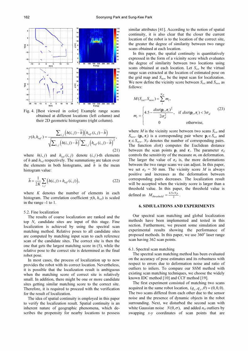
The 2D geometric histogram represents the distribu-tion of the pairwise geometric relationships. To construct 2D geometric histogram of a scan, we vote the distance-angular relationship in (2) in the Hough space (ρ,θ). This generates a pattern which is invariant to rotation and translation of range scan because all the distance-angular relationships are defined relative to local reference frame of each scan point. Fig. 4 shows examples of range scans obtained at different locations and their 2D geometric histograms.

In order to compute the similarity measure between input scan and a reference scan, we use the correlation coefficient of their 2D geometric histograms in this paper. Once 2D geometric histograms h and href for input scan and a reference scan are constructed, they can be compared using the histogram correlation function as follows:

Fig. 3. Flowchart of our global localization system.


162

Fig. 4. [Best viewed in color] Example range scans

obtained at different locations (left column) and their 2D geometric histograms (right column).

( )( )

( ) ( )

,

2 2

, ,

( , ) ( , )( , ) ,

( , ) ( , )

refi j

ref

refi j i j

h i j h h i j h

h h

h i j h h i j h

γ

− −

=

− −

∑

∑ ∑

(21) where ( )h i j, and ( )

refh i j, denote (i, j )-th elements

of h and href respectively. The summations are taken over the elements in both histograms, and h is the mean histogram value:

( ),

1( , ) ( , ) ,

2ref

i j

h h i j h i jK

= +∑ (22)

where K denotes the number of elements in each histogram. The correlation coefficient γ(h, href) is scaled in the range -1 to 1.

5.2. Fine localization

The results of coarse localization are ranked and the top Nc candidate sites are input of this stage. Fine localization is achieved by using the spectral scan matching method. Relative poses to all candidate sites are computed by matching input scan to each reference scan of the candidate sites. The correct site is then the one that gets the largest matching score in (5), while the relative pose to the correct site is determined as the final robot pose.

In most cases, the process of localization up to now provides the robot with its correct location. Nevertheless, it is possible that the localization result is ambiguous when the matching score of correct site is relatively small. In addition, there might be one or more candidate sites getting similar matching score to the correct site. Therefore, it is required to proceed with the verification for the result of localization.

The idea of spatial continuity is employed in this paper to verify the localization result. Spatial continuity is an inherent nature of geographic phenomena, which de-scribes the propensity for nearby locations to possess

similar attributes [41]. According to the notion of spatial continuity, it is also clear that the closer the current location of the robot is to the location of the correct site, the greater the degree of similarity between two range scans obtained at each location.

In this paper, the spatial continuity is quantitatively expressed in the form of a vicinity score which evaluates the degree of similarity between two locations using scans obtained at each location. Let Sest be the virtual range scan extracted at the location of estimated pose on the grid map and Snew be the input scan for localization. We now define the vicinity score between Sest and Snew as follows:

2

2

( , ) ,

( , )4 5 , if ( , ) 3

2

0 otherwise,

PN

est new i

i

i i

i i d

i d

M S S m

distdist

mσ

σ

=

⎧. − <⎪

= ⎨⎪⎩

∑

p rp r

(23)

where M is the vicinity score between two scans Sest and Snew. (pi, ri) is a corresponding pair where pi∈Sest and ri∈Snew. NP denotes the number of corresponding pairs. The function dist() computes the Euclidean distance between the scan points pi and ri. The parameter σd controls the sensitivity of the measure mi on deformation. The larger the value of σd is, the more deformations between the two range scans we can adjust. In this paper, we set σd = 50 mm. The vicinity score M is always positive and increases as the deformation between corresponding pairs decreases. The localization result will be accepted when the vicinity score is larger than a threshold value. In this paper, the threshold value is

defined as 4 5

2

PN

thresholdM

. ×

= .

6. SIMULATIONS AND EXPERIMENTS

Our spectral scan matching and global localization

methods have been implemented and tested in this section. Furthermore, we present some simulation and experimental results showing the performance of proposed methods. In this paper, we use 360o laser range scan having 362 scan points.

6.1. Spectral scan matching

The spectral scan matching method has been evaluated on the accuracy of pose estimates and its robustness with respect to errors due to deformation noise and ratio of outliers to inliers. To compare our SSM method with existing scan matching techniques, we choose the widely known IDC method [10] and CCF method [19].

The first experiment consisted of matching two scans acquired in the same robot location, ( , , ) (0,0,0).

x yq q θ =

The two scans differed from each other due to the sensor noise and the presence of dynamic objects in the robot surrounding. Next, we disturbed the second scan with white Gaussian noise (0, ),N σ and added nO outliers by swapping x-y coordinates of scan points that are


163

randomly selected in the second scan. We set 10σ = and 60.

On = The second scan was then applied to a

random pose up to ± 400 mm in tx and ty, and up to ± 30o in θ. The two scans which are misaligned with each other by a pose ( 400mm, 30 )

x yt t θ= = =

� are shown in Fig. 5(a). The initial pose and misaligned pose are denoted by circles with arrows. The results of correcting the pose error and aligning the two scans with our method appear in Fig. 5(b). We repeated the experiment 500 times in this scenario. Table 1 depicts the mean and standard deviations of the pose errors from the SSM, IDC, and CCF methods. It can be seen that the pose errors from SSM are quite small compared with the other two methods. These statistical results indicate that our scan matching method is robust and accurate.

The second experiment evaluated the robustness of matching performance. The first scan used in the first experiment was applied as the first scan in the second experiment. We obtain the second scan by disturbing the first scan with white Gaussian noise, and then rotating and translating randomly, and next adding outliers in the same manner as the first experiment. Fig. 6 shows the

performance curves of the SSM method vs. the IDC method. Both algorithms ran over 30 trials on the same problem scans for each parameter value on the x axis. The matching rates (correctly matched inliers/total inliers) are obtained by averaging the 30 tests. The proposed method proves to be more robust than the IDC method to deformation noises or the presence of outliers. This is because each correct correspondence can estab-lish pairwise relationships with other correct corre-spondences even in the presence of pairwise relation-ships with incorrect correspondences.

6.2. Global localization with simulations

We verified the performance of proposed global localization method by simulations. All laser range scans for localization tests were extracted with the ray-casting operation at randomly selected positions on a grid map. Thus, we can exactly know the ground truth values to compare with the results of localization tests. Two types of simulations were conducted. The first evaluated the performance of proposed global localization method in detail. The second evaluated the accuracy of robot pose estimation.

Fig. 7(a) shows the grid map for the simulation, which is the Intel Research Lab having a size 60 m×60 m. From the grid map, we constructed the GVD and detected the reference sites such as shown in Fig. 7(b). The number of detected reference sites was 321. The reference scans at the positions of all reference sites were then extracted with the ray-casting operation.

The first simulation consisted of performing global localization at a random location. On the grid map in Fig. 7(a), we selected a random position and extracted virtual range scan. Fig. 8 shows the virtual range scan extracted at the test location and its 2D geometric histogram. Since we chose the test position on the grid map, the ground truth pose was clearly known: ( , , ) (6513.79mm,

x yq q θ =

17519.64mm, 122.58 ).−

� We performed the proposed global localization

method with the virtual range scan in Fig. 8. Table 2 shows the results of global localization. The number of candidate sites was 54 according to (20) but we indicate the results from top 10 candidate sites in this table. Here, the vicinity score was computed with the range scan for localization and the reference scan of each candidate site. The local pose indicates the relative pose to the reference frame of each reference site. It can be transformed with respect to one global coordinates system (e.g., reference frame of the grid map) since the reference frame of reference site is defined relative to the global coordinates system. We denote the transformed local pose as global pose.

Among the all candidate sites, reference site 181 obtained the largest spectral matching score as well as vicinity score. Furthermore, the distance between the ground truth and the global pose defined through reference site 181 was the smallest. Therefore, reference site 181 was determined to be the correct site. Fig. 9 shows the range scan of reference site 181 and its 2D geometric histogram. We can identify that the 2D

(a) Misaligned two scans

before scan matching. (b) Aligned two scans after

scan matching.

Fig. 5. Two scans used in the evaluation experiment of SSM. Red points for the first scan and blue points for the second scan with outliers.

Table 1. Mean (μ) and standard deviation (σ) of estimat-ed pose errors with SSM, IDC, and CCF methods.

x error [mm] y error [mm] θ error [o]

μ σ μ σ μ σ

SSM 0.27 10.51 -0.42 7.99 0.01 0.09

IDC 5.77 215.61 -30.69 259.82 0.69 14.18

CCF -91.00 105.84 -123.80 196.90 0.51 13.90

(a) 72 outliers, varying de-

formation noise. (b) Deformation noise σ =

5, varying ratio of out-liers to inliers.

Fig. 6. Performance curves for SSM method vs. IDC method.


164

geometric histogram of the range scan for localization is similar to that of reference site 181 even though ranges scans in Figs. 8 and 9 are rotated and translated relative to each other.

In order to proceed with the verification of the localization result, we computed the vicinity score with the range scan for localization and virtual range scan extracted at the correct global pose (6507.18 mm,

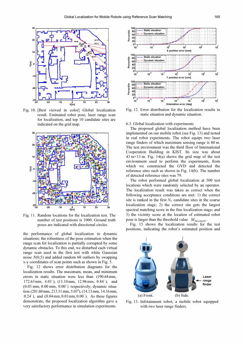
17534.28 mm, –122.65o). The vicinity score was 1611.77 and we therefore accepted the localization result because the vicinity score was larger than the threshold value Mtheshold. Fig. 10 depicts the result of global localization on the grid map and locations of candidate sites. We can also clearly see that the range scan for localization is remarkably matched with the grid map and reference site 181 is nearest to the robot.

The second simulation focused on verifying the accuracy of pose estimation in the grid map of the Intel Research Lab. For this simulation, a total of 1000 different test positions were randomly chosen from the whole grid map. Fig. 11 shows the test locations, which indicates the robot’s positions and orientations relative to its environment with directional circles.

For each test location in Fig. 11, we performed two types of tests. The first test conducted global localization with virtual range scans extracted at the test locations, which assumed that the environment is static, i.e., there were no dynamic obstacles. The second test evaluated

Fig. 8. [Best viewed in color] Range scan for localization test in a static situation (left) and its 2D geometric histogram (right).

Fig. 9. [Best viewed in color] Range scan of reference site 181 (left) and its 2D geometric histogram(right).

(a)

(b)

Fig. 7. (a) Grid map of the Intel Research Lab. (b) GVD constructed from the grid map and reference sites. Red lines represent the GVD and black circles indicate the reference sites. The number of reference sites is 321.

Table 2. Results of global localization performed with the range scan in Fig. 8. Candidate site 181 183 190 168 205 194 199 198 213 313

Correlation coefficient 0.7986 0.7457 0.7448 0.7397 0.6889 0.6747 0.6733 0.6665 0.6625 0.6612

Spectral matching score 4958.96 3083.39 2366.148 4225.71 680.05 656.67 843.19 705.89 276.13 396.02

Vicinity score 604.21 587.75 524.86 427.71 200.36 176.87 133.34 152.01 216.32 187.86

Local

pose

xL [mm] -992.82 -2183.03 -4108.03 2128.93 -5676.96 -3355.65 6488.08 834.14 1843.85 -774.01

yL [mm] 1234.28 1111.18 1931.09 -1466.92 -2377.63 -1672.51 201.13 178.42 484.06 714.91

θL[o] -122.65 -122.51 -122.37 -122.35 -161.53 -0.05 22.32 -144.77 -129.59 -132.93

Global

pose

xG [mm] 6507.18 6516.97 6491.97 6528.93 11023.04 8844.35 20188.08 14334.14 20843.85 18225.99

yG [mm] 17534.28 17511.18 17531.09 17533.08 4022.37 7227.49 10401.13 9878.42 17984.06 20914.91

θG [o] -122.65 -122.51 -122.37 -122.35 -161.53 -0.05 22.32 -144.77 -129.59 -132.93

Error

| qx – xG | 6.61 3.18 21.82 15.14 4509.25 2330.56 13674.29 7820.35 14330.06 11712.20

| qy – yG | 14.61 8.46 11.45 13.44 13497.27 10292.15 7118.51 7641.22 464.42 3395.27

| θ – θG | 0.07 0.07 0.21 0.23 38.95 122.53 144.90 22.19 7.01 10.35


165

the performance of global localization in dynamic situations: the robustness of the pose estimation when the range scan for localization is partially corrupted by some dynamic obstacles. To this end, we disturbed each virtual range scan used in the first test with white Gaussian noise N(0,5) and added random 60 outliers by swapping x-y coordinates of scan points such as shown in Fig. 5.

Fig. 12 shows error distribution diagrams for the localization results. The maximum, mean, and minimum errors in static situation were less than (190.68mm, 172.63mm, 4 01 ),.

�

(13.10mm, 12.96mm, 0.84 ),� and

(0.03 mm, 0.00 mm, 0.00 )� respectively; dynamic situa-

tion (201.60 mm, 213.51 mm, 5.03o), (14.13 mm, 14.16 mm, 0.24 ),

� and (0.04mm,0.01mm,0.00 ).� As these figures demonstrate, the proposed localization algorithm gave a very satisfactory performance in simulation experiments.

Fig. 12. Error distribution for the localization results in

static situation and dynamic situation.

6.3. Global localization with experiments The proposed global localization method have been

implemented on our mobile robot (see Fig. 13) and tested in real robot experiments. The robot equips two laser range finders of which maximum sensing range is 80 m. The test environment was the third floor of International Cooperation Building in KIST. Its size was about 43 m×13 m. Fig. 14(a) shows the grid map of the test environment used to perform the experiments, from which we constructed the GVD and detected the reference sites such as shown in Fig. 14(b). The number of detected reference sites was 79.

The robot performed global localization at 500 test locations which were randomly selected by an operator. The localization result was taken as correct when the following acceptance conditions are met: 1) the correct site is ranked in the first NC candidate sites in the coarse localization stage; 2) the correct site gets the largest spectral matching score in the fine localization stage; and 3) the vicinity score at the location of estimated robot pose is larger than the threshold value .

thresholdM

Fig. 15 shows the localization results for the test positions, indicating the robot’s estimated position and

Fig. 10. [Best viewed in color] Global localization

result. Estimated robot pose, laser range scan for localization, and top 10 candidate sites are indicated on the grid map.

Fig. 11. Random locations for the localization test. The

number of test positions is 1000. Ground truth poses are indicated with directional circles.

(a) Front. (b) Side.

Fig. 13. Infotainment robot, a mobile robot equipped with two laser range finders.


166

orientation relative to its environment. The correct ratios of the coarse localization are shown in Fig. 16. It describes that all of the correct sites were ranked in the first ten candidate sites. More specifically, 471 correct

sites were ranked among the first five candidate sites; 301 correct sites ranked first. Fig. 17 shows the distribution of vicinity score for the localization results. The maximum, mean, and minimum score were 1358.18, 1322.40, and 1216.74, respectively. As can be seen from the figures, all of the localization results satisfied the acceptance conditions, accordingly we can identify the proposed global localization method gave good perfor-mance in real indoor environment.

7. CONCLUSION

In this paper, we presented a new approach for scan

matching-based global localization of mobile robots. This aims to estimate relative pose to the most likely reference site by matching input scan with reference scans.

Our approach uses the spectral scan matching method based on pairwise geometric relationships. These geometric relationships are formed by fully connected scan points, and they are invariant with respect to translation and rotation of range scan, so that the spectral scan matching method can be applicable in both structured and unstructured environments even if range scans are corrupted by dynamic obstacles. And further-more, the spectral scan matching method can estimate robot’s pose without knowing initial pose, which allows mobile robots to estimate their poses with no wandering behaviors. In this respect, our work also can give the problem of path planning a solution for setting up an initial position.

The proposed global localization system consists of two stages: coarse localization and fine localization. The coarse localization results ranked in the top list are given as candidate sites for the next stage. The fine localization determines the correct site and estimates robot’s pose relative to the correct site. This coarse-to-fine framework enhances the efficiency and accuracy of global localiza-tion.

We have implemented our approach on a mobile robot, and tested in simulations and real robot experiments. Tests performed with our method in two different environments have demonstrated that it could be accurate and effective approaches to mobile robot navigation.

(a)

(b) Fig. 14. (a) Grid map of the third floor of International

Cooperation Building in KIST. (b) GVD constructed from the grid map and reference sites. Red lines represent the GVD and black circles indicate the reference sites. The number of reference sites is 79.

Fig. 15. Localization results for different locations in the test environment. The estimated poses of the robot are indicated with directional circles.

Fig. 16. Correct ratio of coarse localization. The correct site is ranked in the first x (horizontal axis) of candidate sites.

Fig. 17. Distribution of vicinity score for the localiza-tion results in Fig. 15.


167

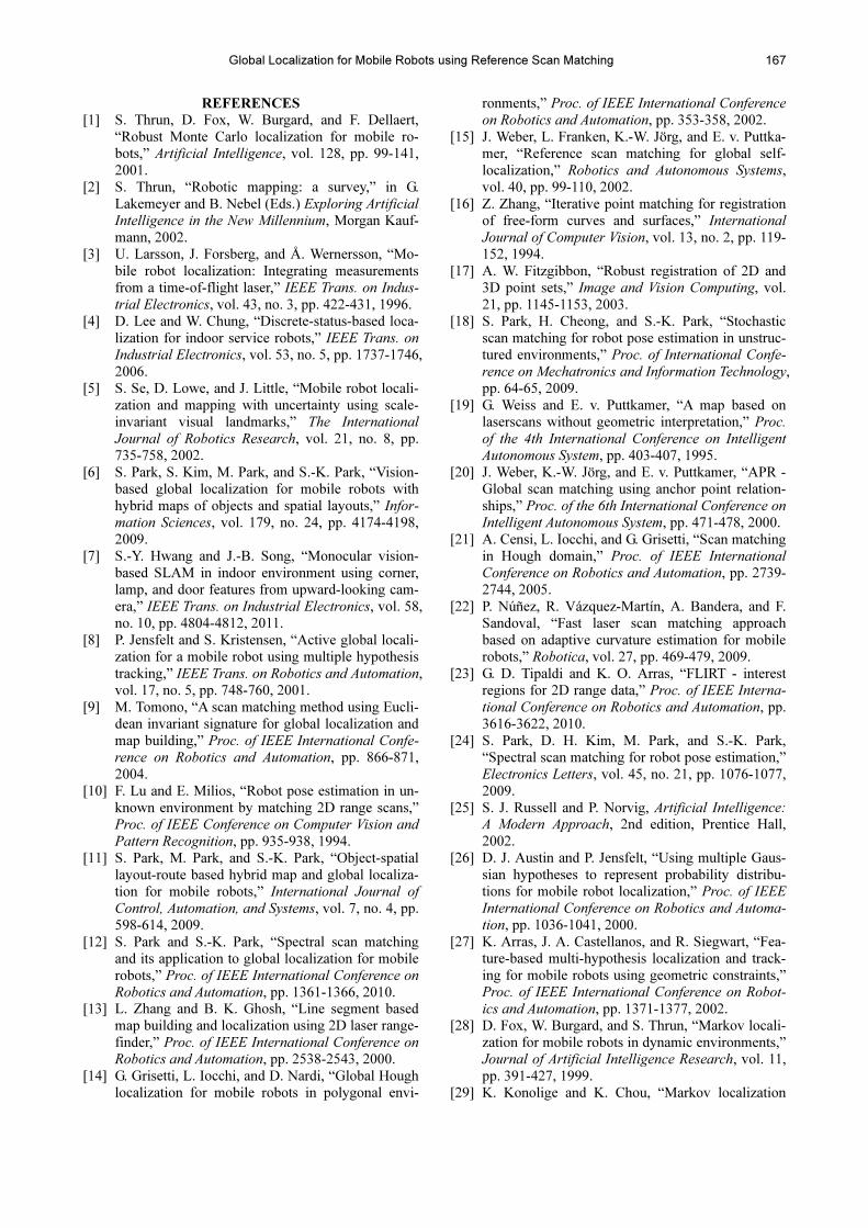
REFERENCES

[1] S. Thrun, D. Fox, W. Burgard, and F. Dellaert, “Robust Monte Carlo localization for mobile ro-bots,” Artificial Intelligence, vol. 128, pp. 99-141, 2001.

[2] S. Thrun, “Robotic mapping: a survey,” in G. Lakemeyer and B. Nebel (Eds.) Exploring Artificial

Intelligence in the New Millennium, Morgan Kauf-mann, 2002.

[3] U. Larsson, J. Forsberg, and Å. Wernersson, “Mo-bile robot localization: Integrating measurements from a time-of-flight laser,” IEEE Trans. on Indus-

trial Electronics, vol. 43, no. 3, pp. 422-431, 1996. [4] D. Lee and W. Chung, “Discrete-status-based loca-

lization for indoor service robots,” IEEE Trans. on

Industrial Electronics, vol. 53, no. 5, pp. 1737-1746, 2006.

[5] S. Se, D. Lowe, and J. Little, “Mobile robot locali-zation and mapping with uncertainty using scale-invariant visual landmarks,” The International

Journal of Robotics Research, vol. 21, no. 8, pp. 735-758, 2002.

[6] S. Park, S. Kim, M. Park, and S.-K. Park, “Vision-based global localization for mobile robots with hybrid maps of objects and spatial layouts,” Infor-

mation Sciences, vol. 179, no. 24, pp. 4174-4198, 2009.

[7] S.-Y. Hwang and J.-B. Song, “Monocular vision-based SLAM in indoor environment using corner, lamp, and door features from upward-looking cam-era,” IEEE Trans. on Industrial Electronics, vol. 58, no. 10, pp. 4804-4812, 2011.

[8] P. Jensfelt and S. Kristensen, “Active global locali-zation for a mobile robot using multiple hypothesis tracking,” IEEE Trans. on Robotics and Automation, vol. 17, no. 5, pp. 748-760, 2001.

[9] M. Tomono, “A scan matching method using Eucli-dean invariant signature for global localization and map building,” Proc. of IEEE International Confe-

rence on Robotics and Automation, pp. 866-871, 2004.

[10] F. Lu and E. Milios, “Robot pose estimation in un-known environment by matching 2D range scans,” Proc. of IEEE Conference on Computer Vision and

Pattern Recognition, pp. 935-938, 1994. [11] S. Park, M. Park, and S.-K. Park, “Object-spatial

layout-route based hybrid map and global localiza-tion for mobile robots,” International Journal of

Control, Automation, and Systems, vol. 7, no. 4, pp. 598-614, 2009.

[12] S. Park and S.-K. Park, “Spectral scan matching and its application to global localization for mobile robots,” Proc. of IEEE International Conference on

Robotics and Automation, pp. 1361-1366, 2010. [13] L. Zhang and B. K. Ghosh, “Line segment based

map building and localization using 2D laser range-finder,” Proc. of IEEE International Conference on

Robotics and Automation, pp. 2538-2543, 2000. [14] G. Grisetti, L. Iocchi, and D. Nardi, “Global Hough

localization for mobile robots in polygonal envi-

ronments,” Proc. of IEEE International Conference

on Robotics and Automation, pp. 353-358, 2002. [15] J. Weber, L. Franken, K.-W. Jörg, and E. v. Puttka-

mer, “Reference scan matching for global self-localization,” Robotics and Autonomous Systems, vol. 40, pp. 99-110, 2002.

[16] Z. Zhang, “Iterative point matching for registration of free-form curves and surfaces,” International

Journal of Computer Vision, vol. 13, no. 2, pp. 119-152, 1994.

[17] A. W. Fitzgibbon, “Robust registration of 2D and 3D point sets,” Image and Vision Computing, vol. 21, pp. 1145-1153, 2003.

[18] S. Park, H. Cheong, and S.-K. Park, “Stochastic scan matching for robot pose estimation in unstruc-tured environments,” Proc. of International Confe-

rence on Mechatronics and Information Technology, pp. 64-65, 2009.

[19] G. Weiss and E. v. Puttkamer, “A map based on laserscans without geometric interpretation,” Proc.

of the 4th International Conference on Intelligent

Autonomous System, pp. 403-407, 1995. [20] J. Weber, K.-W. Jörg, and E. v. Puttkamer, “APR -

Global scan matching using anchor point relation-ships,” Proc. of the 6th International Conference on

Intelligent Autonomous System, pp. 471-478, 2000. [21] A. Censi, L. Iocchi, and G. Grisetti, “Scan matching

in Hough domain,” Proc. of IEEE International

Conference on Robotics and Automation, pp. 2739-2744, 2005.

[22] P. Núñez, R. Vázquez-Martín, A. Bandera, and F. Sandoval, “Fast laser scan matching approach based on adaptive curvature estimation for mobile robots,” Robotica, vol. 27, pp. 469-479, 2009.

[23] G. D. Tipaldi and K. O. Arras, “FLIRT - interest regions for 2D range data,” Proc. of IEEE Interna-

tional Conference on Robotics and Automation, pp. 3616-3622, 2010.

[24] S. Park, D. H. Kim, M. Park, and S.-K. Park, “Spectral scan matching for robot pose estimation,” Electronics Letters, vol. 45, no. 21, pp. 1076-1077, 2009.

[25] S. J. Russell and P. Norvig, Artificial Intelligence:

A Modern Approach, 2nd edition, Prentice Hall, 2002.

[26] D. J. Austin and P. Jensfelt, “Using multiple Gaus-sian hypotheses to represent probability distribu-tions for mobile robot localization,” Proc. of IEEE

International Conference on Robotics and Automa-

tion, pp. 1036-1041, 2000. [27] K. Arras, J. A. Castellanos, and R. Siegwart, “Fea-

ture-based multi-hypothesis localization and track-ing for mobile robots using geometric constraints,” Proc. of IEEE International Conference on Robot-

ics and Automation, pp. 1371-1377, 2002. [28] D. Fox, W. Burgard, and S. Thrun, “Markov locali-

zation for mobile robots in dynamic environments,” Journal of Artificial Intelligence Research, vol. 11, pp. 391-427, 1999.

[29] K. Konolige and K. Chou, “Markov localization


168

using correlation,” Proc. of International Joint

Conference on Artificial Intelligence, pp. 1151-1159, 1999.

[30] J. Reuter, “Mobile robot self-localization using PDAB,” Proc. of IEEE International Conference on

Robotics and Automation, pp. 3512-3518, 2000. [31] M. Isard and A. Blake, “Condensation - conditional

density propagation for visual tracking,” Interna-

tional Journal of Computer Vision, vol. 29, no. 1, pp. 5-28, 1998.

[32] S.-K. Park, M. Kim, and C.-W. Lee, “Mobile robot navigation based on direct depth and color-based environment modeling,” Proc. of IEEE/RSJ Inter-

national Conference on Intelligent Robots and Sys-

tems, pp. 4253-4258, 2004. [33] M. Leordeau and M. Hebert, “A spectral technique

for correspondence problems using pairwise con-straints,” Proc. of International Conference on

Computer Vision, pp. 1482-1489, 2005. [34] P. J. Rousseeuw and A. M. Leroy, Robust Regres-

sion and Outlier Detection, Wiley, 2003. [35] S. Kumar, Models for Learning Spatial Interactions

in Natural Images for Context-Based Classification, Ph.D. Thesis, The Robotics Institute, Carnegie Mel-lon University, 2005.

[36] K. Lange, Numerical Analysis for Statisticians, Springer, 1999.

[37] R. A. Horn and C. R. Johnson, Matrix Analysis, Cambridge University Press, 1985.

[38] J. H. Challis, “A procedure determining rigid body transformation parameters,” Journal of Biomechan-

ics, vol. 28, no. 6, pp. 733-737, 1995. [39] H. Choset, K. Lynch, S. Hutchinson, G. Kantor, W.

Burgard, L. Kavraki, and S. Thrun, Principles of

Robot Motion: Theory, Algorithms, and Implemen-

tation, MIT Press, 2005. [40] J.-C. Latombe, Robot Motion Planning, Kluwer

Academic Publishers, 1991. [41] M. F. Goodchild, “Geographical information

science,” International Journal of Geographical In-

formation Systems, vol. 6, no. 1, pp. 31-45, 1992.

Soonyong Park received his B.S. and

M.S degrees in Mechanical Engineering

from Kyunghee University, Seoul, Korea,

in 2001 and 2003, respectively. He re-

ceived his Ph.D. degree in Electrical and

Electronic Engineering from Yonsei Uni-

versity, Seoul, Korea, in 2010. From

2001 to 2010, he was a graduate student

researcher and a postdoctoral fellow with

the Cognitive Robotics Center, Korea Institute of Science and

Technology (KIST), Seoul, Korea. He was a postdoctoral fel-

low with the Robotics Institute, Carnegie Mellon University

(CMU), in 2011. From 2012 to 2013, he was a research staff

member in the Samsung Advanced Institute of Technology

(SAIT) at Samsung Electronics. He is now a senior engineer in

the Global Technology Center at Samsung Electronics. His

research interests include computer vision, machine learning,

and mobile robot navigation.

Sung-Kee Park is a principal research

scientist for Korea Institute of Science

and Technology (KIST). He received his

B.S. and M.S. degrees in Mechanical

Design and Production Engineering from

Seoul National University, Seoul, Korea,

in 1987 and 1989, respectively. He re-

ceived his Ph.D. degree from Korea Ad-

vanced Institute of Science and Technol-

ogy (KAIST), Korea, in the area of computer vision in 2000.

Since then, he has been studying the field of robot vision and

cognitive robotics at KIST. During his period at KIST, he held

a visiting position in the Robotics Institute at Carnegie Mellon

University (CMU) in 2005, where he did research on object

recognition. Now he is working for the center of Bionics at

KIST. His recent work has been on object recognition, visual

navigation, video surveillance, human-robot interaction, and

socially assistive robot.

Documents

Global localization for mobile robots using reference scan matching