Federal Reserve Bank of Dallas Globalization and Monetary Policy Institute

Working Paper No. 120 http://www.dallasfed.org/assets/documents/institute/wpapers/2012/0120.pdf

Global Banks, Financial Shocks and International Business Cycles:

Evidence from an Estimated Model*

Robert Kollmann ECARES, Université Libre de Bruxelles and CEPR

July 2012

Abstract This paper estimates a two-country model with a global bank, using US and Euro Area (EA) data, and Bayesian methods. The estimated model matches key US and EA business cycle statistics. Empirically, a model version with a bank capital requirement outperforms a structure without such a constraint. A loan loss originating in one country triggers a global output reduction. Banking shocks matter more for EA macro variables than for US real activity. During the Great Recession (2007-09), banking shocks accounted for about 20% of the fall in US and EA GDP, and for more than half of the fall in EA investment and employment. JEL codes: F36, F37, E44, G21

* Robert Kollmann, ECARES, CP 114, Université Libre de Bruxelles; 50 Av. Franklin Roosevelt, B-1050 Brussels, Belgium. 32-2- 650- 4474. robert_kollmann@yahoo.com. Matthias Paustian contributed to this project in its early stages--I thank him for his advice and for computer code. I also thank Werner Roeger for many discussions. Helpful comments and suggestions were also received from Gernot Müller, Alan Sutherland, Christoph Thoenissen, Ken West, Egon Zakrajšek and participants at several workshops. For financial support I thank the National Bank of Belgium, Université Libre de Bruxelles (Action de recherche concertée ARC-AUWB/2010-15/ULB-11) and the EU Commission (CEPR project 'Politics, Economics and Global Governance: The European Dimensions' funded by the EU Commission under its 7th Framework Programme for Research, Contract Nr. 217559.) The views in this paper are those of the author and do not necessarily reflect the views of the Federal Reserve Bank of Dallas or the Federal Reserve System.

2

1. Introduction

The global financial crisis that erupted in 2007 revealed the fragility of major financial

institutions, and it led to the sharpest global recession since the 1930s. These dramatic

events require a rethinking of the role of financial intermediaries for real activity. Before

the crisis, standard macro theory largely abstracted from financial intermediaries. The

crisis has stimulated much research that incorporates banks in dynamic stochastic general

equilibrium (DSGE) models. Given the global nature of the crisis, that research has

frequently focused on open economy models; see, for example, Devereux and Sutherland

(2011), Gamber and Thoenissen (2011), and Kollmann et al. (2011).1 In this new class of

DSGE models, bank capital is a key state variable for domestic and foreign real

activity—negative shocks to bank capital are predicted to increase the spread between

banks’ lending and deposit rates, and to trigger a fall in bank credit and real activity; with

a globalized banking system, a loan loss originating in one country can thus lead to a

worldwide recession.

So far, this new open economy macro-banking literature has used calibrated

models--a systematic quantitative empirical assessment of the role of banks as a source of

shocks and as a transmission channel in the global economy has not yet been presented.

In order to provide such an assessment, the present paper estimates (using Bayesian

methods) a two-country DSGE model with a global bank. Quarterly US and Euro Area

(EA) macro data and banking data (bank loans, bank capital ratio and loan spread) for the

period 1990-2010 are used. 2

The model here assumes that each country is inhabited by a (representative)

worker, an entrepreneur and a government. The global bank collects deposits from

workers and makes loans to entrepreneurs, in both countries. The bank has to finance a

fraction of her assets using equity (own funds). This constraint can reflect legal

requirements and, more broadly, market pressures. It implies that the loan rate spread 1 See also Correa et al. (2010), Davis (2010), Nguyen (2011), Andreasen et al. (2010), Perri and Quadrini (2011), Ueda (2011) and Van Wincoop (2011). Closed economy DSGE models with banks were, i.a., presented by Aikman and Paustian (2006), Van den Heuvel (2008), de Walque et al. (2010), Gertler and Kiyotaki (2011), Del Negro et al. (2011) and Kollmann et al. (2012a,b). 2 Some previous papers have estimated open economy DSGE models, but those studies abstracted from banks. Two-country models were estimated by de Walque et al. (2005), Rabanal and Tuesta (2006) and Le et al. (2010) who also used UE and EA data, and by Jacob and Peersman (2011). Small open economy models were estimated by Adolfson et al. (2009) and Justiniano and Preston (2010).

3

(relative to the deposit rate) is a decreasing function of bank capital, as the marginal

benefit of bank capital is a decreasing function of bank capital. The estimated model

assumes demand and supply shocks in home and foreign labor and good markets. In

addition, there are stochastic loan losses (defaults) in the two countries, and shocks to the

required bank capital ratio—henceforth, I refer to these shocks as ‘banking shocks’.

The estimation results suggest that the bank capital requirement, and the banking

shocks, matter for the dynamics of macro variables. A model with these ingredients

outperforms model variants without an operative bank capital requirement or without

banking shocks. According to the baseline model estimates, a one percentage point fall in

the global bank capital ratio raises the loan rate spread by 44 basis points. An

unanticipated US loan loss of 1$ lowers both US and EA GDP by about 0.15 $, on

impact. An unanticipated increase in the required bank ratio by one percentage point

lowers US and EA GDP by 0.21%, on impact.

The estimated model matches key cyclical properties of US and EA macro and

banking variables. In particular, it captures the fact that US and EA loans are more

volatile than output, and that loans are procyclical, while the loan spread is

countercyclical. It also captures the fact that GDP, consumption, investment and bank

loans are positively correlated across the US and the EA. Banking shocks matter more

for EA macro variables than for US real activity. These shocks account for 5%-10% of

US GDP volatility, and for 10%-25% of US investment and employment volatility. By

contrast, banking shocks, explain 15%-30% of EA GDP volatility, 50%-70% of EA

investment volatility, and 25%-50% of EA employment volatility.

Banking shocks played a noticeable role in the 2007-2009 ‘Great Recession’, but

were not the dominant factor driving the fall in GDP: according to the estimates, banking

shocks accounted for about 20% of the fall in US and EA GDP during that recession;

however, banking shocks accounted for more than half of the fall in EA investment and

employment. During the previous US recession (2001) banking shocks also accounted for

about 25% of the fall in US GDP and investment.

Section 2 presents the model. Section 3 discusses the econometric approach.

Section 4 describes key data features. Section 5 reports the estimation results. Section 6

concludes.

4

2. A two-country world with a global financial intermediary

In each of the two countries, called ‘Home’ (H) and ‘Foreign’ (F), there is a

representative worker, an entrepreneur and a government. A global bank collects deposits

from workers, and makes loans to entrepreneurs, in both countries. The bank faces a

capital requirement: a fraction of bank assets has to be financed using the bank’s own

funds (equity). Entrepreneurs produce a homogenous tradable good that is used for

consumption and for capital accumulation. All agents are infinitely-lived. Markets are

competitive. Preferences and technologies have the same structure in both countries. The

following exposition focuses thus on the Home country. Foreign variables are denoted by

an asterisk.

2.1. Preferences, technologies, markets

The Home worker

The Home worker provides labor to the Home entrepreneur and invests her savings in

one-period bank deposits. Her date t budget constraint is:

1W W Dt t t t t t tC D T N D Rω++ + = + , (1)

where WtC and tN are the worker’s consumption and hours worked respectively. tω is

the real wage rate. 1tD + is the bank deposit held by the worker at the end of period t. DtR

is the gross interest rate on deposits, between t-1 and t. WtT is a lump sum tax. The

worker’s date t expected life-time utility, ,WtV is:

1 1 1( ) ( )W W D N W Wt t t t t t t tV u C u D N E Vβ+ + += +Ψ −Ψ + ,

with 111( ) ( 1),u x x σσ

−−= − 0σ > and 0.DΨ > The worker’s marginal disutility of labor,

0,NtΨ > is an exogenous random variable. N

tΨ will be referred to as the Home labor

supply shock. Note that deposits provide utility to the worker (liquidity services). This

ensures that, in equilibrium, the deposit rate is smaller than the loan rate, and that workers

hold deposits while entrepreneurs borrow. The worker’s subjective discount factor is

decreasing in her future consumption: 1 1( ),W W Wt tCβ β+ +≡ with 10 ( ) 1,W W

tCβ +< < 1' ( ) 0.W WtCβ + <

The subjective discount factors of other agents are likewise decreasing functions of their

5

own consumption.3 Agents treat their subjective discount factors as given, i.e. they do not

internalize the effect of consumption on the discount factor—I thus write the argument of

the subjective discount factor with an upper-bar. It is assumed that all agents have the

same steady state rate of time preference, and the same risk aversion coefficient, .σ

The Home worker maximizes her life-time utility subject to the period-by-budget

constraint (1). That decision problem has these first-order conditions:

'( )W Nt t tu C ω = Ψ , (2)

1 1 1 1'( )/ '( ) '( )/ '( ) 1D W W W Dt t t t t t tR E u C u C u D u Cβ+ + + ++ Ψ = . (3)

The Home entrepreneur

The Home entrepreneur accumulates physical capital and uses capital and local labor to

produce output. Her technology is 1( ) ( ) ,t t t tZ K Nα αθ −= 0 1,α< < where ,t tZ K and tN are

output, capital and labor, respectively. Total factor productivity (TFP), 0,tθ > is an

exogenous random variable. The law of motion of capital stock is 1 (1 ) ,t t t tK K Iδ+ = − +Ξ

where 0 1δ≤ ≤ is the capital depreciation rate and tI is gross investment. 0tΞ > is an

exogenous random shock to investment efficiency (Fischer (2006), Justiniano et al.

(2008)). Gross investment is generated using output. Let ( / )tI I Iξ be the amount of

output needed to generate ,tI where I is steady state investment, and ξ is an increasing,

strictly convex function with '(1) 1.ξ ξ(1)= = Henceforth, variables without time subscripts

denote steady state values. The Home entrepreneur’s period t budget constraint is:

11( / ) ( ) ( )L E E

t t t t t t t t t t t tL R I I N d T L K Nα αξ ω θ −+− Δ + Ι + + + = + , (4)

where tL is a one-period bank loan received by the Home entrepreneur in period t-1. LtR

is the gross interest rate on that loan, set at t-1. In period t, the Home entrepreneur

defaults by an exogenous random amount tΔ on the amount Lt tL R that she owes the

bank. EtT is a lump sum tax. E

td is the entrepreneur’s dividend income at t. The

3 When subjective discount factors are constant, the model has a unit root (due to market incompleteness, transitory shocks then have permanent effects on the agents’ relative wealth). The endogenous discount factors induce mean-reversion in individual wealth, and thus ensures stationarity (Kollmann (1991); Schmitt-Grohé and Uribe (2003)). The numerical solution method (local approximation) and the estimation method require stationarity.

6

entrepreneur consumes her dividend income. Her expected lifetime utility at t, ,EtV is:

1( ) ,E E E Et t t t tV u d E Vβ += + with 1 1( ) 1E E E

t tdβ β+ += < . Utility maximization by the entrepreneur

(subject to (4)) yields these first-order conditions:

(1 )t t t tK Nα αω α θ −= − , (5)

1 1 1'( )/ '( ) 1L E E Et t t t tR E u d u dβ+ + + = , (6)

1 11 1 1 1 1 1( '( )/ '( )){ (1 )} 1/E E E

t t t t t t t t tE u d u d K N q qα αβ θ α δ− −+ + + + + ++ − = , with '( / )/ .t t tq I Iξ≡ Ξ

The Home government

At date t, the Home government makes exogenous random output purchases tG that are

financed using lump sum taxes: ,W E Bt t t tG T T T= + + where B

tT is a tax paid by the bank

(see below). Each Home agent bears a constant share of the total Home tax burden, equal

to her share in Home steady state consumption: i i it tT Gλ= for i=W,E,B where iλ is time-

invariant. In setting taxes, the Home and Foreign governments assume that 50% of the

banker’s consumption takes place in country Home.

The global bank

The paper focuses on the role of bank capital for the transmission of macroeconomic and

financial shocks to global real activity. The paper therefore adopts an aggregate

perspective, and assumes a representative global bank that may be thought of as the

global financial system.4 At t, the global bank receives deposits 1tD + and *1tD + from the

Home and Foreign workers, respectively, and makes loans 1tL + and *

1tL + to Home and

Foreign entrepreneurs, respectively. Let *1 1 1

Wt t tD D D+ + +≡ + and

*1 1 1

Wt t tL L L+ + +≡ + denote

worldwide deposits and loans. The bank faces a capital requirement: her date t capital

4 Thus, the interbank market is not modeled here. Frictions in that market would matter for aggregate activity if they affected the total flow of funds from savers to borrowers. The model here captures empirical fluctuations in the loan spread and in the total volume of intermediation. To investigate the potential role of an interbank market, I studied a model variant with a savings bank and an investment bank. The savings bank gets deposits from households, and lends to the investment bank (interbank market), which lends to firms. Each bank faces a capital requirement and charges a loan spread. However, aggregate dynamics hinges on total bank capital--thus that set-up is observationally equivalent to the representative-bank model.

7

1 1W Wt tL D+ +− should not be smaller than a fraction tγ of the bank’s assets 1.

WtL + This may

reflect a legal requirement or, more broadly, market pressures. 5 tγ is a random variable

that is exogenous to the bank (see below). The bank can hold less capital than the

required level, but this is costly. Let 1 1 1( )W W Wt t t t tx L D Lγ+ + +≡ − − = 1 1(1 ) W W

t t tL Dγ + +− − denote the

bank’s ‘excess’ capital at the end of period t. The bank bears a cost ( / )W WtL x Lφ as a

function of ,tx where WL is the steady state stock of loans. φ is a convex function

( '' 0)φ ≥ for which I assume: ( ) 0txφ > for 0tx < ; (0) 0.φ = Thus, for 0tx < the bank incurs a

positive cost; the cost is zero when the bank meets her capital requirement. At t, the bank

also bears an operating cost 1 1( )W Wt tD L+ +Γ⋅ + , where 0Γ > is the (constant) real marginal

cost of taking deposits and making loans. The bank’s period t budget constraint is:

**1 1 1 1( ) ( / ) ,W W D W W W W B B B W L W

t t t t t t t t t t t t t tL D R D L L x L d T T L R Dφ+ + + ++ + Γ⋅ + + + + + = −Δ −Δ +

where *t tΔ +Δ is the bank’s total loan loss, and *B B

t tT T+ is the total tax paid by the bank

(in the two countries). Btd is the profit (dividend) generated by the bank at t. (As the bank

acts competitively, loan rates and deposit rates are equated across countries.) The banker

consumes her dividend income. Her expected life-time utility at t, ,BtV is:

1 1( ) ,B B B Bt t t t tV u d E Vβ + += + with 1 1( ) 1B B B

t tdβ β+ += < .

The banker’s utility maximization problem has these first-order conditions:

1 1 1'( )/ '( ) 1 'D B B Bt t t t t tR E u d u dβ φ+ + + = − Γ + ,

1 1 1'( )/ '( ) 1 (1 ) '( / )L B B B Wt t t t t t tR E u d u d x Lβ γ φ+ + + = + Γ + − .

A linear approximation of these Euler equations gives:

1 1 2 ( / ) 2 (0) (0) ( / )''' 'L D W Wt t t t t tR R x L x Lγ φ γ φ γφ+ +− ≅ Γ− ≅ Γ− − ⋅ . (7)

Hence, the loan rate spread 1 1L Dt tR R+ +− is a function of the required capital ratio tγ and of

the bank’s excess capital, .tx Note that if the bank raises deposits and loans by one unit,

then her operating cost rises by 2Γunits; excess bank capital falls by ,tγ which raises the

5 Bank capital requirements are often justified as limiting moral hazard in the presence of informational frictions and deposit insurance (see Freixas and Rochet (2008)). These issues are not explicitly modeled here. Instead, I take the capital requirement as given, and focus on its macroeconomic effects.

8

penalty ( / )W WtL x Lφ by ( / )' W

t tx Lγ φ− . The bank’s Euler equations imply that the spread

between the loan rate and the deposit rate 1 1L Dt tR R+ +− covers the marginal cost

2 ( / )' Wt tx Lγ φΓ− . Under strict convexity of φ (i.e. 0),''φ > the marginal benefit of excess

capital 'φ− is a decreasing function of (excess) bank capital, which implies that the loan

rate spread is likewise a decreasing function of excess bank capital.

The sensitivity of the loan rate spread to changes in bank capital is governed by

''.φ Note that / ,Wt t tx L cr γ≅ − where 1 1 1( )/W W W

t t t tcr L D L+ + +≡ − is the bank’s capital ratio, i.e.

the ratio of bank equity to bank assets. A one percentage point rise in the capital ratio

lowers the loan rate spread by 4 ''γφ percentage points per annum (p.a.), while a one

percentage point increase in the required bank capital ratio (holding constant tcr ) raises

the spread by 4[ '' ']γφ φ− percentage points p.a..

Market clearing

Market clearing for the output good requires: * * * * * * *

1 1( / ) ( / ) / ).( ) (E E B W W W Wt t t t t t t t t t t t t tZ Z C C d d d I I I I I I G G L x L L Dξ ξ φ + ++ = + + + + + + + + + +Γ⋅+

Forcing variables

Steady state TFP and investment efficiency are normalized to unity * *( 1).θ θ= =Ξ=Ξ =

There are 11 forcing variables: Home and Foreign TFP *( , )t tθ θ , investment efficiency

*( , ),t tΞ Ξ government purchases *( , )t tG G , labor supply shocks *( , )N Nt tΨ Ψ , loan losses

*( , )t tΔ Δ and the required bank capital ratio ( ).tγ I refer to the first 8 shocks are ‘non-

banking’ shocks, and to the last three shocks as ‘banking shocks’. A large number of non-

banking shocks is assumed so that the model has the potential to capture important

features of macro data, even in the absence of banking shocks. Other recent estimated

DSGE models likewise assume many shocks (e.g., Smets and Wouters (2007)).

Following the empirical DSGE literature, I assume that each ‘non-banking’ shock

tz follows a stationary univariate AR(1) process:

1ln( / ) ln( / )z zt t tz z z zρ ε−= + , (8)

9

with 0 1zρ≤ < , where ztε is a normally distributed white noise. The innovations to the

non-bank shocks are correlated. Let nbktε denote the vector of innovations to the 8 non-

banking shocks.

The laws of motion of loan losses (normalized by steady state GDP) and of the

required bank capital ratio are:

1/ / ln( / )t t t tY Y Y Yρ ϑ εΔ Δ Δ−Δ = Δ + + , * * * * * * * *

1/ / ln( / ) ,t t t tY Y Y Yρ ϑ εΔ Δ Δ−Δ = Δ + + (9)

1(1 ) ln( / )W Wt t t tY Yγ γ γ γγ ρ γ ρ γ ϑ ε−= − + + + , (10)

with *0 , , 1.γρ ρ ρΔ Δ≤ < tY , *tY and *W

t t tY Y Y≡ + are Home and Foreign GDP and world

GDP respectively.6 tεΔ , *

tεΔ and t

γε are normal white noises. tεΔ and *

tεΔ are correlated,

but independent of tγε . *( , , )bk

t t t tγε ε ε εΔ Δ≡ is assumed independent of the vector of non-

banking shocks, ,nbktε at all leads and lags. To allow for correlation between *( , , )t t tγΔ Δ

and the non-banking forcing variables, I assume that *( , , )t t tγΔ Δ depends on GDP and

thus is partly endogenous. The independence of nbktε and bk

tε makes it straightforward to

decompose the variance of the endogenous variables into components due to nbktε and to

,bktε respectively (see below).

2.2 Model solution

A linear approximation (around the deterministic steady state) is used to solve the model.

The solution can be expressed as

1 1 2t t ts s ε−=Λ +Λ , (11)

where ts is a vector consisting of states and controls chosen (or realized) in period t,

expressed as deviations from steady state values. ( , )nbk bkt t tε ε ε≡ is the vector of date t

6 The bank’s operating costs and the costs of excess bank capital ( / )W W

tL x Lφ represent inputs used by the bank; these costs thus have to be subtracted from the entrepreneurs’ output when computing GDP. I assume that the resources used by Home banking 1 1)( t tL D+ ++Γ⋅ are purchased from the Home entrepreneur, and that 50% of the resource cost ( / )W W

tL x Lφ is likewise purchased from the Home entrepreneur. Hence, Home GDP is: 1

1 1 2( ) ( / ).W Wt t t t tY Z L D L x Lφ+ +≡ −Γ + −

10

innovations to the forcing variables. 1Λ and 2Λ are matrices whose elements are

functions of the model parameters.

3. Econometric approach

The model is estimated using quarterly time series for 12 macro and banking variables, in

1990q1-2010q3: US and EA GDP, total private consumption, investment, employment,

commercial bank credit (deflated using the GDP deflator), the loan rate spread of US

commercial banks, and the capital ratio of US commercial banks. The baseline estimates

use data on total bank credit (to all sectors) by US Commercial banks and by EA

Monetary financial institutions (MFI). Below, I also report estimation results that instead

use data on credit to the business sector. (I use total credit for the baseline estimates, as

that variable accounts for a greater share of bank assets.) The measure of the US loan rate

spread is the series ‘commercial and industrial loan rates spread over intended federal

funds rate’, from the Federal Reserve Board’s (FRB) Survey of Terms of Business

Lending (Table E.2). Data on the EA loan rate spread are only available for the period

since 2003q1; as shown in Figure 2, the available EA loan spread closely tracks the US

loan spread (correlation in 2003-2010: 0.90).7 I thus use the US loan rate spread as a

measure of the global loan rate spread. The US Commercial bank capital ratio is taken as

a proxy for the capital ratio of the global bank. The empirical bank capital ratio measure

is constructed as (total financial assets – total liabilities)/total financial assets, using data

from the Flow of Funds (FRB). See the Appendix for further information on the

empirical variables. In estimation, the loan spread and the capital ratio are demeaned,

while the other empirical variables are linearly detrended in log-form.

The number of data series used for estimation (12) exceeds the number of shocks

(11). To avoid stochastic singularity of the model, I assume that observed variables

contain measurement error. Allowing for measurement error also seems important

because (especially) the empirical banking series might be imperfect measures of the

7 The EA spread plotted in Fig. 2 is the difference between the EA MFI loan rate and the EONIA rate.

11

theoretical concepts.8 The date t data used in estimation, ,obsty are a subset of the states

and controls included in the vector ts (see (11)), and are measured with error:

,obst t ty s μ=Γ + (12)

where Γ is a matrix, and tμ is a vector of Gaussian i.i.d. measurement errors that are

independent of the true state variables at all leads and lags. I use a Bayesian approach to

estimate a subset of the parameters, while the remaining parameters are calibrated.

3.1. Estimated and calibrated parameters

I estimate the following parameters: the curvature of the bank capital penalty function

'',φ the curvature of the investment cost function '',ξ and the parameters of the process

governing the banking shocks (9),(10). These parameters are key for the dynamic

properties of the model, but do not affect the steady state. In addition, I estimate the risk

aversion coefficient ,σ and the standard deviations of measurement errors.

I calibrate the remaining parameters so that the steady state matches long run

properties of the data. E.g. the technology parameter 1 α− is set at the mean empirical

labor share, the steady state bank capital ratio is calibrated using historical mean capital

ratios etc. It would be difficult to estimate these parameters through the lens of the model,

unless ratios of the relevant variables were used in the measurement equation (as pointed

out by Smets and Wouters (2007)). In addition, I calibrate the non-banking shock

processes.

3.1.1. Prior parameter distribution

The means and standard deviations of prior parameter distributions are shown in Cols.

(1)-(2) of Table 3. The mean of the prior distribution of σ is set at unity. ''φ affects the

response of the loan rate spread to changes in the bank capital ratio, and is thus key for

the transmission of banking shocks to real activity. Recall that a one percentage point

8To break the singularity, measurement error in just one observable is sufficient. To determine the presence of measurement error empirically, I allow for it in all series. Assuming measurement error just in banking variables gives the same results about the role of banking shocks. For recent empirical DSGE models that explicitly allow for measurement error see Ireland (2004), Boivin and Giannoni (2006), Gali et al. (2011) and de Antonio (2011).

12

increase in the bank capital ratio lowers the loan rate spread by 4 ''γφ percentage points

per annum. As discussed below, I set the steady state required bank capital ratio at

0.117.γ= I set the mean of the prior distribution at 4 ''γφ at 0.2, a value consistent with

time series regressions of the loan rate spread on aggregate bank capital reported by

Kollmann et al. (2011). Investment is excessively volatile when the capital accumulation

technology is linear ( '' 0),ξ = as then international capital flows respond very rapidly to

country-specific shocks. I set the mean of the prior distribution of ''ξ at 1; for that value,

the ratio of the standard deviation of investment divided by the standard deviation of

GDP is about 3 in the different model variants discussed below, and thus roughly in the

range of the relative volatility of EA investment, when the other parameters are set at

prior mean values. 9

The priors of the parameters of the banking shock processes (9),(10) are set as

follows: the prior mean of the standard deviations of *,t tε εΔ Δ and tγε is 0.5%; the prior

mean of the correlation between tεΔ and *

tεΔ and of the autoregressive coefficients

*, , γρ ρ ρΔ Δ is 0.5; the prior mean of the GDP coefficients, ϑΔ and ,γϑ is 0.10 The prior

mean of the standard deviation of *, gt tε εΔ and t

γε is in the range of estimated standard

deviations of innovations to empirical measures of the non-banking shocks--see

discussion below (e.g. the historical standard deviation of US and EA TFP innovations is

0.48%, see Table 1). Empirically, TFP and other non-banking shocks (except the labor

supply shock) are positively correlated across countries—the prior thus assumes that loan

losses are likewise positively correlated across countries. The prior means and prior

standard deviations of the standard deviations of measurement errors are set at 1/4 and

1/20, respectively, of the standard deviations of the corresponding (demeaned/detrended)

empirical series.

9 The prior distributions of , ''σ φ and ''ξ are Gamma distributions with standard deviations set at half the prior means. Thus a reasonably wide range of parameter values around the mean has non-negligible mass. 10 The prior standard deviations of these parameters are set at 0.1.

13

3.1.2. Calibration

Calibrated technology parameters (non-finance sector), size of government

One period in the model represents one quarter in calendar time. As is standard in the

macro literature, the (quarterly) depreciation rate of physical capital is set at δ=0.025.

The elasticity of output with respect to capital is set at α=0.3, consistent with long run

average historical US and EA labor shares of about 70%.

The two-country model here abstracts from US and EA trade with third countries;

I thus use the sum of US government consumption and of US net exports to countries

other than the EA as an empirical measure of US ‘autonomous’ spending, ;tG EA

autonomous spending is constructed analogously. During 1990-2010, US [EA]

autonomous spending represented 14.2% of US GDP [21.2% of EA GDP], on average. I

take the US as the empirical counterpart of country ‘Home’ and set / 14.2%,G Y=

* */ 21.2%.G Y =

Calibrated preference and bank parameters

Most DSGE studies calibrate the subjective discount factor to match average historical

returns. I use the same approach. As mentioned above, it is assumed that all agents have

the same steady state subjective discount factor, here denoted by .β β is set so that the

steady state loan rate matches the mean 1990-2010 US real loan rate. I use the interest

rate on ‘commercial and industrial loans made by all commercial banks’ reported by the

FRB (Survey of Terms of Business Lending, Table E.2) as a measure of the nominal loan

rate, from which I subtract the quarterly growth rate of the US GDP deflator to construct

the real loan rate. The average US real loan rate 1990-2010 was 3.440% p.a..

Accordingly, I set the (quarterly) steady state subjective discount factor at 0.9918β = (as

1,LRβ = from the entrepreneur’s Euler equation (6)).

I assume that all agents’ subjective discount factors have the same elasticity with

respect to consumption, denoted by .βε I set βε at a small absolute value, 0.001,βε = −

that yields a stationary equilibrium, while generating (essentially) the same short run

dynamics as a model variant with a constant subjective discount factor. (Impulse

14

responses over the first 100 periods are very similar across model variants with 0βε =

and 0.001.)βε = −

The sample mean (1990-2010) of the US loan rate spread was 2.161% p.a..11 I set

the steady state deposit rates in the model at 1.279% p.a., so that the steady state loan rate

spread matches the mean historical spread, 2.161%. The mean EA loan spread was 2.01%

in 2003-2010 (see above), which is close to the steady state spread assumed in the model

calibration.

I set the steady state actual and required bank capital ratios at 11.17%,cr γ= =

which corresponds to the average capital ratio of US commercial banks during the sample

period (from Flow of Funds data). The bank’s Euler equations imply 1 'DR β φ= −Γ+ and

1 (1 ) .'LR β γ φ= +Γ+ − Given the steady state deposit and loan rates, these two conditions

pin down the bank’s marginal operating cost Γ and the steady state slope of the bank’s

‘penalty’ function ' :φ 0.25%, ' 0.28%.φΓ= = −

The assumption that cr γ= implies that steady state excess bank capital is zero,

x=0, i.e. (1 ) .W WL Dγ− = I set (1 )L Dγ− = and * *(1 ) ,L Dγ− = i.e. the steady state ratio of

deposits to loans is the same in both countries (as is consistent with the data). The ratio of

outstanding US commercial bank loans to annual US GDP was 53% on average in 1990-

2010, while the mean ratio of the stock of EA MFI loans divided by annual EA GDP was

87%. Thus, the US has a noticeably lower loans/GDP ratio than the EA. The calibration

reflects this: I assume that the steady state ratios of loans to annual GDP are 53% in

country ‘Home’, and 87% in ‘Foreign’. Finally, I assume that both countries have the

same steady state GDP, normalized at unity: * 1.Y Y= = These steady state targets pin

down the remaining preference parameters (the weights of deposits in Home and Foreign

11 As mentioned above, the baseline measure of the US loan rate spread is the ‘commercial and industrial loan rates spread over intended federal funds rate’. Using the rate on short term Certificates of Deposit as a measure of the bank’s marginal funding costs yields a loan rate spread that has a 0.75 correlation with the baseline spread, and a sample mean of 1.929% p.a., which is close to the assumed steady state spread.

15

workers’ utility functions, *,D DΨ Ψ , and steady state marginal disutilities of labor,

*, ).N NΨ Ψ 12

Calibrated ‘non-banking’ shock processes.

I construct quarterly empirical measures of the 8 US and EA ‘non-banking’ forcing

variables (1990-2010). Following Coeurdacier, Kollmann and Martin (2010), I use the

ratio of the CPI to the investment deflator as a measure of investment efficiency. The

empirical labor supply shock is constructed as (1 )( / )/ ,Nt t t tZ N CαΨ = − which follows from

the first order conditions (2),(5) when 1σ = (i.e. when σ equals its prior mean). Thus, the

empirical labor supply shock is proportional to labor productivity divided by

consumption.13

I set the standard deviations, and auto- and cross-correlations of the non-banking

shocks in the model equal to the corresponding moments of linearly detrended logs of the

empirical measures (see Table 1). The empirical DSGE literature--that has largely

focused on closed economies--typically assumes uncorrelated shocks, and it estimates the

parameters of shock processes through the lens of the DSGE model (jointly with the

remaining parameters). In a multi-country model it is important to allow for correlated

shocks—empirical measures of the shocks are strongly correlated. I calibrate the process

governing non-banking shocks, as empirical measures of the non-banking shocks can

easily be constructed, and as estimation of the correlation matrix of these shocks through

the lens of the model would be challenging (given the large number of cross-

correlations).

As reported in Table 1, US investment efficiency, US autonomous spending and

the US labor supply shock are more volatile than the corresponding EA variables. The

cross-country correlations of TFP (0.51) and investment efficiency (0.84) are sizable. 12 (3) implies (1 )(( / )/( / )) .D D WR C Y D Y σβ −Ψ = − /D Y is determined by / ,L Y while /WC Y is pinned down by ratios of government purchases and investment to GDP. 1Y= then pins down NΨ (as NΨ determines the steady state labor input). In steady state, consumption by the Home [Foreign] worker and the entrepreneur represent respectively 58.2% and 4.8% [52.3% and 3.5%] of domestic GDP, while the banker’s consumption represents 0.21% of world GDP. 13 Labor productivity is constructed using GDP as a proxy for the entrepreneur’s output Z. I also considered an alternative measure of the labor supply shock based on real wage rate data: / .N

t t tCωΨ = That measure gives similar estimates of model parameters and of the role of banking shocks.

16

TFP is positively correlated with investment efficiency; US and EA TFP are strongly

negatively correlated with US autonomous spending (G), and negatively correlated with

the US labor supply shock. All forcing variables are highly persistent (autocorrelations in

the range 0.80-0.98).

4. Data plots and business cycle statistics.

Figure 1 plot the (demeaned/detrended) 12 empirical series used in estimation. Macro

aggregates co-move closely across the US and the EA—the synchronicity was especially

high during the recent ‘Great Recession’. According to the NBER, that recession began

in 2007q4 and ended in 2009q2. (Shaded areas in Figures indicate NBER recessions.)

Relative to trend, US output fell by 8.5%, during the recession, while EA output fell by

7.5%; US consumption (-7.3%) and investment (-35.1%) fell more sharply than EA

consumption (-4.0%) and investment (-15.9%). US and EA bank lending grew strongly in

the years before 2008, and then collapsed sharply. The loan rate spread fell during the

three years prior to the crisis, but rose sharply during the Great Recession. The bank

capital ratio exhibits relatively mild fluctuations--throughout the sample period it stays in

a ±2% range around the sample mean of 11.17%.

Figures 3a-b plot the bank capital ratio, together with the baseline loan spread

series and alternative spread measures that are used for robustness checks below (all

series in Figures 3a-b are demeaned). Except for the period of the financial crisis, the

bank capital ratio and the baseline loan rate spread comove negatively. While the loan

rate spread rose, during the crisis (as mentioned above), the bank capital ratio has had a

flat trend since about 2005--it has been argued that this may partly reflect accounting

discretion, which has allowed banks to overstate the value of their assets in the crisis

(Huizinga and Laeven (2009)). The correlation between the bank capital ratio and the

baseline lending spread was -0.46 during the period 1990-2007, but close to zero (-0.06)

over the whole sample period (1990-2010).

Figure 3a also plots the series ‘net percentage of banks increasing spreads of loan

rates over cost of funds’, from the FRB Senior Loan Officer Opinion Survey on Bank

Lending Practices, SLOOS. (The series represents the percentage of banks increasing

spreads minus the percentage of banks lowering spreads; the plotted series is scaled so

that its standard deviation equals that of the baseline loan spread.) That series is

17

positively correlated with the baseline loan spread (correlation 0.39 for 1990-2010), and

negatively correlated with the bank capital ratio (-0.47 for 1990-2007; -0.21 for 1990-

2010).

Figure 3b plots Gilchrist and Zakrajšek’s (2011a) excess US commercial bond

premium, constructed by subtracting expected bond default probabilities from the spread

between the yield on US commercial bonds and the yield on US Treasury bonds.14 As

commercial banks are key players in the commercial bond market, the commercial bond

premium might be informative about credit spreads/market conditions.15 The excess bond

premium too is negatively correlated with the bank capital ratio (correlation: -0.49 for

1990-2007; -0.15 for 1990-2010). The bond premium is positively correlated with the

baseline loan rate spread (0.29) and with the SLOOS ‘net percentage of banks increasing

spreads’ (0.79).

Overall, the data are thus consistent with the model’s prediction that the spread is

inversely related to the bank capital ratio (see (7)). The absence of an pronounced inverse

relation during the crisis might be due to the fact that the measured bank capital ratio

overstates the true capital ratio during the crisis (see discussion above), or that the

required bank capital ratio rose during the crisis (this could rationalize the observed

increase in the loan rate spread, during the crisis, without a fall in the bank capital ratio).

Table 2 reports moments of Hodrick-Prescott (HP) filtered macro and banking

variables, for the US and the EA (1990-2010). GDP volatility is very similar in the US

(1.12%) and the EA (1.14%). Consumption is less volatile than GDP, while investment is

markedly more volatile than GDP. US investment is almost twice as volatile as EA

investment. In both ‘countries’, loans are more volatile than output, while the loan spread

is countercyclical. Real activity and loans are positively correlated across the US and EA.

14 I thank Egon Zakrajšek for providing me with the excess bond premium series, and with the business loan and loan capacity data used below. 15 Gilchrist and Zakrajšek (2011a) argue that ‘an increase in the excess bond premium reflects [...] a contraction of the supply of credit with significant adverse consequences for the macroeconomy’ (p.31).

18

5. Estimation results

5.1. Posterior parameter estimates (Table 3)

Columns (4)-(6) of Table 3 respectively report the means, the modes and the standard

deviations of the posterior parameter distribution, for the baseline model (posterior means

and modes are very close); Cols. (7) and (8) show the 5th and 95th percentiles of the

posterior parameter distributions. 16

The data are informative about the estimated parameters: in almost all cases, the

posterior parameter distributions have lower standard deviations than the prior

distributions; the posterior means often differ noticeably from the prior means. The

posterior estimate (mode) of 4 ''γφ indicates that a 1 percentage increase in the bank

capital ratio leads to a 44 basis point reduction in the annualized loan rate spread, and that

a 1 percentage point rise in the required bank capital ratio ( )tγ increases the loan rate

spread by 45 basis points p.a..

The posterior estimates also show that EA loan loss shocks are more volatile than

US loan loss shocks—the posterior modes of the standard deviations of tεΔ and *

tεΔ are

0.48% and 1.38%, respectively. US and EA loan loss shocks are positively correlated

(0.34). The required bank capital ratio undergoes sizable fluctuations (posterior mode of

std. of :γε 0.53%). The posterior means of the standard deviations of measurement errors

are mostly smaller than the prior means. An important exception to this is the sizable

standard deviation of measurement error for bank capital ratio (its posterior mode is

1.31%). 17

5.2. Business cycle moments implied by posterior estimates (Table 4)

Table 4 reports model-predicted moments of HP filtered US and EA variables, computed

at the posterior mode of the estimated parameters. Column (1) assumes all 11 structural

shocks, and measurement error. Cols. (2)-(9) consider moments generated by different

subsets of the structural shocks, in isolation, without measurement error. Specifically,

16The means, standard deviations and deciles of the posterior distributions were generated using the Random Walk Metropolis algorithm (see An and Schorfheide (2007)). 17 The estimated measurement error for the bank capital ratio is markedly smaller when the model is estimated using data on business loans; see below.

19

Col. (2) assumes just the 8 non-banking shocks ,nbktε and Col. (3) assumes just the 3

exogenous banking shocks .bktε Cols. (4)-(9) assume just a single type of shock (Col.(4):

just TFP shocks; Col. (5): just investment efficiency shocks; etc.). Col. (10) reports

empirical moments (from Table 2). 18

The model with all shocks and measurement error generates predicted statistics

that are mostly in the range of the empirical statistics. The predicted standard deviation of

US GDP (1.30%) and of EA GDP (0.88%) are close to the empirical standard deviations.

The model (with all shocks) captures the fact that investment and loans are more volatile

than GDP. The model also matches the empirical cross-correlations of most variables

with domestic GDP—in particular, it correctly predicts that US and EA loans are

procyclical, and that the loan spread is countercyclical. Also, the model correctly predicts

that GDP, consumption, investment and loans are positively correlated across the two

countries—the predicted cross-country correlation of GDP is 0.44.

Taken in isolation, TFP shocks and Labour supply shocks induce by far the

largest fluctuations in real activity (predicted standard deviation of US and EA GDP with

just these shocks: 0.94% and 0.77%, respectively). The predicted standard deviations of

US GDP with just loan loss shocks and with just shocks to the required bank capital ratio

are 0.28% and 0.15%, respectively. With just TFP shocks, just investment efficiency

shocks, and just labor supply shocks, GDP is negatively correlated across countries. By

contrast, government purchases shocks and the banking shocks induce positive cross-

country output correlations. Notice also that the banking shocks induce a strong negative

correlation between the loan rate spread and GDP. Panel (a1) of Table 7 reports the % shares of the predicted variances of HP

filtered endogenous variables (with measurement error) that are accounted for by the non-

banking shocks nbktε (see rows labeled ‘NonBk’), and by the banking shocks bk

tε (rows 18 Using (11),(12), the model solution for observables (with measurement error) can be written as: obs

ty = ( ) ( )nbk bk

t t tA L B Lν νε ε μ− −+ + where ( )A L and ( )B L are lag polynomials. (The moments in Table 4 pertain to HP filtered series, , ( ) ,obs HP obs

t ty H L y= where ( )H L is the HP filter.) By assumption, ,nbk bkt tε ε and tμ are

independent at all leads and lags. Thus the predicted variance of endogenous variables under all shocks and measurement error (Col. (1) of Table 4) is the sum of: (i) the variance with just non-banking shocks (Col.(2)); (ii) the variance with just banking shocks (Col. (3)); (ii) the variance of measurement error. By contrast, the variances predicted under the different individual shocks in Cols. (4)-(10) of Table 4 do not add up to the variance with all shocks, as individual shocks are correlated.

20

labeled ‘Bank’); the remainder represents the contribution of measurement error to the

predicted variance. (The variance shares are computed at the posterior mode of the

estimated parameters.)

According to the baseline model, the banking shocks account for a 6% share of

US GDP variance, but explain larger shares of the variances of US investment (11.3%

share), employment (15.2%) and loans (28.1%). Banking shocks account for roughly 2-5

times larger variance shares of EA variables--GDP: 15.5%; investment: 55.1%;

employment: 26.5%; loans: 76.3%. Thus, more than half of the variance of EA

investment and loans is due to banking shocks. 19

5.3. Impulse responses (Table 5)

Impulse responses (reported in Table 5) help to understand the model’s mechanics, and

the predicted business cycle moments. The impulse responses are computed at the

posterior mode of estimated model parameters. Each impulse response focuses on an

isolated innovation, assuming that all other exogenous innovations are zero.20 A positive

innovation to Home TFP raises Home GDP and investment, but leads to a fall in Foreign

GDP and investment. The shock raises the income of the Home worker; thus that worker

saves more, and her holdings of bank deposits increase--i.e. the bank’s debt rises, which

lowers the bank capital ratio. This raises the loan rate spread. The deposit rate falls (due

to the greater supply of deposits); the Foreign worker responds to this by consuming

more, and working less, and hence Foreign GDP falls. Foreign investment falls likewise,

as the reduction in Foreign hours worked lowers the marginal product of capital.

Country-specific investment efficiency shocks and labor supply shocks likewise

drive Home and Foreign GDP in opposite directions. By contrast, banking shocks induce

responses of real activity (and of loans) that are common across the two countries. For

example, a rise in the Home loan loss lowers the global bank’s capital ratio, which

triggers a rise in the loan rate spread; in response to this, loans, investment and GDP fall

in both countries. A rise in the required capital ratio ( )tγ likewise raises the loan rate

19 Banking shocks account for 85.5% of the variance of the loan rate spread, but for only 13.7% of the variance of bank capital, which reflects the sizable estimated measurement error in that variable. 20 To save space, Table 5 does not show responses to EA ‘non-banking’ shocks—those responses are qualitatively similar to the responses to US ‘non-banking’ shocks (reported in Table).

21

spread (see (7)); on impact, this too lowers loans, investment and real activity in both

countries. Note also that banking shocks drive the loan spread and output in opposite

directions. According to the baseline estimates, an unanticipated US loan loss of 1$

lowers both US and EA GDP by about 0.15 $, on impact. An unanticipated increase in

the required bank ratio by one percentage point lowers US and EA GDP by 0.21%, on

impact.

5.4. Decomposing historical time series (Figure 4)

Figure 4 plots the contributions of the banking shocks and of US and EA non-banking

shocks to the historical time series (the decomposition is computed at the posterior mode

of the estimated parameters). 21 Thick continuous lines show the historical data; the thin

continuous lines indicate the contribution of banking shocks, while the dashed-dotted and

dashed lines represent the contributions of US and EA non-banking shocks, respectively.

The historical decomposition yields a picture that is consistent with the variance

decompositions. Banking shocks matter more for EA GDP than for US GDP. Banking

shocks are key drivers of EA investment and employment. During the 2007q4-2009q2

recession, banking shocks account for a 1.6% (1.7%) fall in US (EA) GDP—i.e. the

banking shocks capture about 1/5 of the fall in US GDP (-8.5%) and in EA GDP (-7.5%),

relative to trend. Banking shocks also capture 25% [30%] of the fall in US investment

[employment], and 60% [85%] of the fall in EA investment and employment. Thus, the

fall in EA employment can almost fully be accounted for by banking shocks.

In the previous US recession (2001q1-2001q4), banking shocks accounted for 1/4

of the fall in US output and investment, for 1/3 of the fall in EA output and for 2/3 of the

fall in EA investment. During the 1990q3-1991q1 US recession, the role of banking

shocks was more muted, accounting for 1/10 of the fall in US GDP and investment (the

EA did not experience a recession in 1990-91).

Figure 4 shows that the output components accounted for by the domestic non-

banking shocks track historical US and EA GDP very closely.22 Foreign non-banking

21 Using smoothed shocks and measurement errors, each historical series can be expressed as the sum of: (i) a ‘base’ trajectory (dynamic effects of predetermined states in the initial period) plus measurement error; (ii) contributions of each exogenous shock. Figure 4 shows the data and the shock contributions. 22 This result parallels the finding by de Walque et al. (2005) and Le et al. (2010) that domestic macro shocks are the main drivers of US and EA GDP.

22

shocks had a stabilizing effect on domestic real activity; eg, during the 2007-09

recession, EA non-banking shocks had a positive influence on US GDP, and thus

mitigated the US recession. This reflects the fact that, in the model here, TFP shocks and

labor supply shocks are negatively transmitted internationally (see above).

5.5. Alternative empirical measures of banking variables

As a robustness check, I estimated the model using other empirical measures of the loan

rate spread and of bank loans. Panels (a2)-(a5) of Table 7 report resulting estimates of

variance shares explained by banking shocks. These variance shares are higher, by up to a

factor of 3, than the baseline shares discussed above (Panel (a1)). 23 (Posterior parameter

estimates obtained from the alternative data sets are in the same range as the baseline

estimates, and are thus not reported)

Alternative proxies for the loan rate spread

In Panels (a2) of Table 7, the baseline loan rate spread is replaced by the series ‘net

percentage of banks increasing spreads of loan rates over cost of funds’ (from SLOOS),

while Panel (a3) uses the Gilchrist-Zakrajšek (2011a) excess bond premium series. When

the Gilchrist-Zakrajšek excess bond premium is used, 9.2% (21.8%) of the variance of

US (EA) GDP is due to banking shocks. 24

Business loans and lending capacity

In Panel (a4), total bank credit is replaced by US and EA bank loans to the non-financial

business sector, while Panel (a5) uses Gilchrist and Zakrajšek’s (2011b) measure of US

‘business lending capacity’ in lieu of US total credit.25 Figures 5a-b plot these series.

Business loans are highly positively correlated with total loans, but more volatile,

23 I also estimated the model using an alternative measure of the bank capital ratio--the capital ratio of US Securities Brokers and Dealers (instead of the capital ratio of US commercial banks). Results are robust to using this measure. Kollmann and Zeugner (2012) analyze the capital ratio dynamics of different sub-sectors of the finance industry. 24 Using the SLOOS series ‘net percentage of banks tightening lending standards’ in lieu of the baseline lending spread yields very similar estimated variance shares. 25 Gilchrist and Zakrajšek (2011b) point out that, in the US, many business loans are offered under prior commitment (credit lines); hence, business loans respond with a lag to shocks to bank funding. The Gilchrist and Zakrajšek ‘business lending capacity’ measure is defined as the sum of loans outstanding and of unused commercial bank lending commitments--the authors argue that this variable is more informative (than loans outstanding) for identifying loan supply shifts (no comparable measure exists for the EA).

23

especially in the US. US lending capacity fell earlier and much more sharply than total

lending, during the 2007-09 recession. When these alternative lending (capacity) series

are used, then about 10% of US GDP variance and 25%-30% of EA GDP variance is

attributed to the banking shocks.26

The following conclusions can be drawn from the robustness analysis in Table 7:

Banking shocks matter more for EA macro variables than for US real activity. These

shocks account for 5%-10% of the unconditional volatility of US GDP, and for 10%-25%

of US investment and employment volatility. Banking shocks explain 15%-30% of EA

GDP volatility, 50%-70% of EA investment volatility and 25%-50% of EA employment

volatility. 27

5.6. The role of the bank capital requirement

The presence of an operative bank capital requirement '' 0φ > is key for the transmission

of banking shocks to real activity. Banking shocks have a negligible effect on real

activity, but remain important drivers of loans and the bank capital ratio, when '' 0.φ =

Columns (9)-(11) of Table 3 reports posterior parameter estimates for a model variant

with '' 0φ = (the priors for parameter other than ''φ are the same as in the baseline

model). 28 Table 6 reports the implied predicted business cycle moments, while Panel (b)

of Table 7 shows the corresponding variance shares accounted for by non-banking/

banking shocks.

In the absence of an operative bank capital requirement ( '' 0),φ = the predicted

standard deviations of GDP, investment and the loan rate spread generated by banking

shocks are negligible (0.02% or less); by contrast, non-banking shocks trigger bigger

26 Banking shocks now also account for a much larger share of the variance of the bank capital ratio (above 60%); this is due to the fact that the estimated standard deviation of measurement error in the bank capital ratio (0.4%) is noticeably smaller than when total credit is used in estimation (1.3%). 27 Nolan and Thoenissen (2009) and Jermann and Quadrini (2012) use closed economy models with collateral-constrained firms (but without banks) to construct estimates of shocks to firms’ funding constraints. The authors argue that those shocks can explain up to half of the variance of US GDP. By contrast, the model here assumes that only the bank faces a collateral constraint. 28 The posterior estimate of the investment technology curvature parameter is basically the same as in the baseline model, but the estimated risk aversion coefficient is slightly lower (0.57). The estimated variability of EA loan losses is again greater than that of US loan losses.

24

fluctuations of real activity, than in the baseline model (with an operative bank capital

requirement). Recall that, in the baseline model, a positive TFP shock leads to an increase

in the loan rate spread—the rise in the spread dampens thus the rise in GDP triggered by

that shock. When '' 0,φ = the dampening effect of the loan spread response is not present

anymore—and real activity responds more strongly to TFP changes (and the other non-

banking shocks). With all simultaneous shocks (and measurement error), the predicted

standard deviations of GDP, investment and employment are thus higher than in the

baseline model—and higher than the corresponding empirical statistics.

Model fit can be evaluated using the marginal data density, MDD (marginal

likelihood).29 The log MDD of the baseline model is 3309.78, while the log MDD of the

model variant without the operative bank capital constraint is 3156.99. This implies a

Bayes factor (ratio of posterior odds to prior odds) of 152.79e that massively favors the

baseline model. I also estimated a model variant with an operative bank capital

requirement, but without banking shocks; that model has a log MDD of 3141.43, a value

markedly below the log MDD of the baseline model (with banking shocks).30 This

suggests that both the operative bank capital requirement and the banking shocks help the

model to capture the dynamics of the macro and banking variables used in estimation.

Importantly, the presence of these model ingredients specifically helps to better explain

the 8 US and EA macro variables used in estimation. For these 8 macro variables, the

baseline model has a log MDD of 2211.57, while the model variant without an operative

bank capital requirement (but with banking shocks) has a log MDD of 2031.49. The

model with an operating bank capital requirement, but no banking shocks has a log MDD

of 2108.36. Thus, the bank capital requirement and the banking shocks both help explain

the macro series better.

29 The MDD measures the out-of-sample predictive ability of the model (Geweke (2001)). The MDDs reported below were computed with the Geweke (1999) harmonic mean estimator, using the parameter draws from the Random Walk Metropolis algorithm (An and Schorfheide (2007)) 30 A model variant without an operative bank capital requirement and without banking shocks has a log MDD of 3118.98.

25

6. Conclusion

This paper has estimated a two-country model with a global banking system, using US

and Euro Area (EA) data (1990-2010), and Bayesian methods. The estimated model

matches key US and EA business cycle statistics. Empirically, a model version with an

operative bank capital constraint outperforms a structure without such a constraint. A

loan loss originating in one country triggers a global output reduction. Banking shocks

matter more for EA macro variables than for US real activity. These shocks account for

5%-10% of US GDP volatility, and for 10%-25% of US investment and employment

volatility. Banking shocks, explain 15%-30% of EA GDP volatility, 50%-70% of EA

investment volatility, and 25%-50% of EA employment volatility. During the Great

Recession (2007-09), banking shocks accounted for about 20% of the fall in US and EA

GDP, but for more than half of the fall in EA employment and investment.

26

DATA APPENDIX A.1 Baseline data set used for estimation ● US GDP, private consumption (total), investment (all at constant prices): from US National Income and Product Accounts (Bureau of Economic Analysis, BEA); the investment series include private and government investment. ● US employment: ‘Total nonfarm payrolls: all employees’ (Bureau of Labor Statistics) ● US bank loans: outstanding ‘total bank credit’ by Commercial Bank, deflated using GDP deflator (from June 2011 Flow of Funds, Table L109). ● US bank capital ratio: (total financial assets-total liabilities)/(total financial assets) for Commercial Banks (from June 2011 Flow of Funds, Table L109). ● US loan rate spread: ‘Commercial and industrial loan rates spread over intended federal funds rate’ (‘All loans’ series, Survey of Terms of Business Lending, Table E.2, Federal Reserve Board, June 2011). ● EA GDP, private consumption (total), investment (all at constant prices): from ECB Area-Wide Model (AWM) database (10th update, September 2010). ● EA employment: from AWM database. ● EA bank loans: MFI loans to private sector (from ECB monthly bulletin), deflated using the GDP deflator. A.2 Other variables (used for estimation of model variants) ● Excess bond premium: spread between the yield on US commercial bonds and the yield on Treasury bonds, minus expected bond default probabilities, as constructed by Gilchrist and Zakrajšek (2011a) using data for a panel of individual bonds. ● ‘Net percentage of banks increasing spreads of loan rates over cost of funds’: percentage of banks increasing spreads minus the percentage of banks lowering spreads, from the Senior Loan Officer Opinion Survey on Bank Lending Practices, SLOOS (Federal Reserve Board). SLOOS reports a series (net percentages of banks raising spreads) for loans to ‘large and middle-market firms’ and one for loans to ‘small firms’. The two series are very similar (correlation: 0.95). I use the average of the two series. ● US business loans: outstanding commercial bank loans to the non-financial business sector, constructed by Gilchrist and Zakrajšek (2011b). ● EA business loans: MFI loans to non-financial corporations(NFC), from ECB monthly bulletin, deflated using the GDP deflator. ● US business lending capacity: outstanding commercial bank loans plus unused commercial bank lending commitments (credit lines) to the non-financial business sector, constructed by Gilchrist and Zakrajšek (2011b). A.3 Other variables (used for model calibration) ● ‘Autonomous spending’ (G): government purchases plus net exports to third countries (deflated using GDP deflator). Data sources: AWM, BEA and ECB monthly bulletin. ● Investment efficiency: measured as ratio of CPI to Gross Investment Deflator (BEA and AWM). All series are quarterly and seasonally adjusted (when relevant)

27

REFERENCES Adolfson, M., S. Laséen, J. Lindé and M. Villani, 2007. Bayesian Estimation of an Open

Economy DSGE Model with Incomplete Pass-Through. Journal of International Economics 72, 481-511.

Aikman, D. and M. Paustian, 2006. Bank Capital, Asset Prices and Monetary Policy. Working Paper No. 305, Bank of England.

An, S. and F. Schorfheide, 2007. Bayesian Analysis for DSGE Models. Econometric Reviews 26, 113-172.

Andreasen, M., J. Sondergaard and M. Paustian, 2010. Portfolio Linkages, Financial Shocks and International Business Cycles. Working Paper, Bank of England.

Boivin, J., and M. Giannoni, 2006. DSGE Models in a Data Rich Environment. Working Paper No. 12772, National Bureau of Economic Research.

Coeurdacier, N., R. Kollmann and P. Martin, 2010. International Portfolios, Capital Accumulation and the Dynamics of Capital Flows. Journal of International Economics 80, 100-112.

Correa, R., H. Sapriza and A. Zlate, 2010. International Banks, the Interbank Market, and the Cross-Border Transmission of Business Cycles. Working Paper, International Finance Section, Federal Reserve Board.

Davis, S., 2010. The Adverse Feedback Loop and the Effects of Risk in both the Real and Financial Sectors. Working Paper No. 66, Globalization and Monetary Policy Institute.

de Antonio, D., 2011. What are Shocks Capturing in DSGE Modelling? Noise Versus Structure. Working Paper, National Bank of Belgium.

Devereux, M. and A. Sutherland, 2011. Evaluating International Financial Integration Under Leverage Constraints. European Economic Review 55, 427-442.

Del Negro, M., G. Eggertsson, A. Ferrero, A. and N. Kiyotaki, 2011. The Great Escape? A Quantitative Evaluation of the Fed’s Liquidity Facilities. Staff Report no. 520, Federal Reserve Bank of New York.

de Walque, G, O. Pierrard and A. Rouabah, 2010. Financial (In)Stability, Supervison and Liquidity Injection: A Dynamic General Equilibrium Approach. Economic Journal 120, 1234-1261.

de Walque, G., F. Smets and R. Wouters, 2005. An Estimated Two-Country DSGE Model for the Euro Area and the US Economy. Working Paper, National Bank of Belgium.

Fisher, J., 2006. The Dynamic Effects of Neutral and Investment-Specific Technology Shocks. Journal of Political Economy, Vol 114 No. 3, pp. 413-52.

Freixas, X. and J.-C. Rochet, 2008. The Microeconomics of Banking. MIT Press, Cambridge.

Galí, J., F. Smets and R. Wouters, 2011. Unemployment in an Estimated New Keynesian Model. Working Paper 17084, National Bureau of Economic Research.

Gamber, G. and C. Thoenissen, 2011. Financial Intermediation and the International Business Cycle: the Case of a Small Country with Big Risk. Working Paper, Reserve Bank of New Zealand.

Gertler, M. and N. Kiyotaki, 2011. Financial Intermediation and Credit Policy in Business Cycle Analysis. In: Handbook of Monetary Economics (B. Friedman and M. Woodford, eds.), Vol. 3A, pp.547-599, Elsevier: Amsterdam.

Geweke, J., 1999. Using Simulation Methods for Bayesian Econometric Models: Inference, Development and Communication. Econometric Reviews 18, 1-126.

28

----------, 2001. Bayesian Econometrics and Forecasting. Journal of Econometrics 100, 11-15.

Gilchrist, S. and E. Zakrajšek, 2011a. Credit Spreads and Business Cycle Fluctuations. Working Paper No. 17201, National Bureau of Economic Research.

----------, 2011b. Bank Lending and Credit Supply Shocks, Working Paper, Boston University.

Huizinga, H. and L. Laeven, 2009. Accounting Discretion of Banks During a Financial Crisis. Discussion Papers 7381, Centre for Economic Policy Research.

Ireland, P., 2004. A Method for Taking Models to the Data. Journal of Economic Dynamics and Control 28, 1205-1226.

Jacob, P. and G. Peersman, 2011. Dissecting the Dynamics of the US Trade Balance in an Estimated Equilibrium Model. Working Paper, Ghent University.

Jermann, U. and V. Quadrini, 2012. Macroeconomic Effects of Financial Shocks, American Economic Review 102, 238-271.

Justiniano, A, and B. Preston, 2010. Can Structural Small Open Economy Models Account for the Influence of Foreign Disturbances? Journal of International Economics 81, 61-74.

Justiniano, A, G. Primiceri and A. Tambalotti, 2008. Investment Shocks and Business Cycles. Journal of Monetary Economics 57, 132-145.

Kollmann, R., 1991. Essays on International Business Cycles. PhD Dissertation, University of Chicago.

Kollmann, R., Z. Enders and G. Müller, 2011. Global Banking and International Business Cycles. European Economic Review 55, 407-426.

Kollmann, R. and S. Zeugner, 2012. Leverage as a Predictor of Real Activity and Volatility. Forthcoming in: Journal or Economic Dynamics and Control.

Kollmann, R., W. Roeger and J. in’t Veld, 2012a. Fiscal Policy in a Financial Crisis: Standard Policy versus Bank Rescue Measures. American Economic Review (Papers and Proceedings) 102, 1-7.

Kollmann, R., M. Ratto, W. Roeger and J. in’t Veld, 2012b. Banks, Fiscal Policy and the Financial Crisis. Working Paper, ECARES, Université Libre de Bruxelles.

Le, V., D. Meenagh, P. Minford and M. Wickens, 2010. Two Orthogonal Continents? Testing a Two-Country DSGE Model of the US and the EU Using Direct Inference. Open Economies Review 21, 23-44.

Nguyen, H., 2011. International Crisis Transmission and Asymmetric Recoveries. Working Paper, World Bank.

Nolan, C. and C. Thoenissen, 2009. Financial Shocks and the US Business Cycle. Journal of Monetary Economics 56, 596-604.

Perri, F. and V. Quadrini, 2011. International Recessions. Working Paper, University of Minnesota.

Rabanal, P. and V. Tuesta, 2006. Euro-Dollar Real Exchange Rate Dynamics in an Estimated Two-Country Model: What is Important and What is Not? Working Paper 06/177, International Monetary Fund.

Schmitt-Grohé, S. and M. Uribe, 2003. Closing Small Open Economy Models. Journal of International Economics 61, 163-185.

Smets, F. and R. Wouters, 2007. Shocks and Frictions in US Business Cycles: A Bayesian DSGE Approach. American Economic Review 97, 586-660.

29

Ueda, K., 2010. Banking Globalization and International Business Cycles. Working Paper, Institute for Monetary and Economic Studies, Bank of Japan.

Van den Heuvel, S., 2008. The Welfare Cost of Bank Capital Requirements. Journal of Monetary Economics 55, 298-320.

Van Wincoop, E., 2011. International Contagion Through Leveraged Financial Institutions. Working Paper, University of Virginia.

30

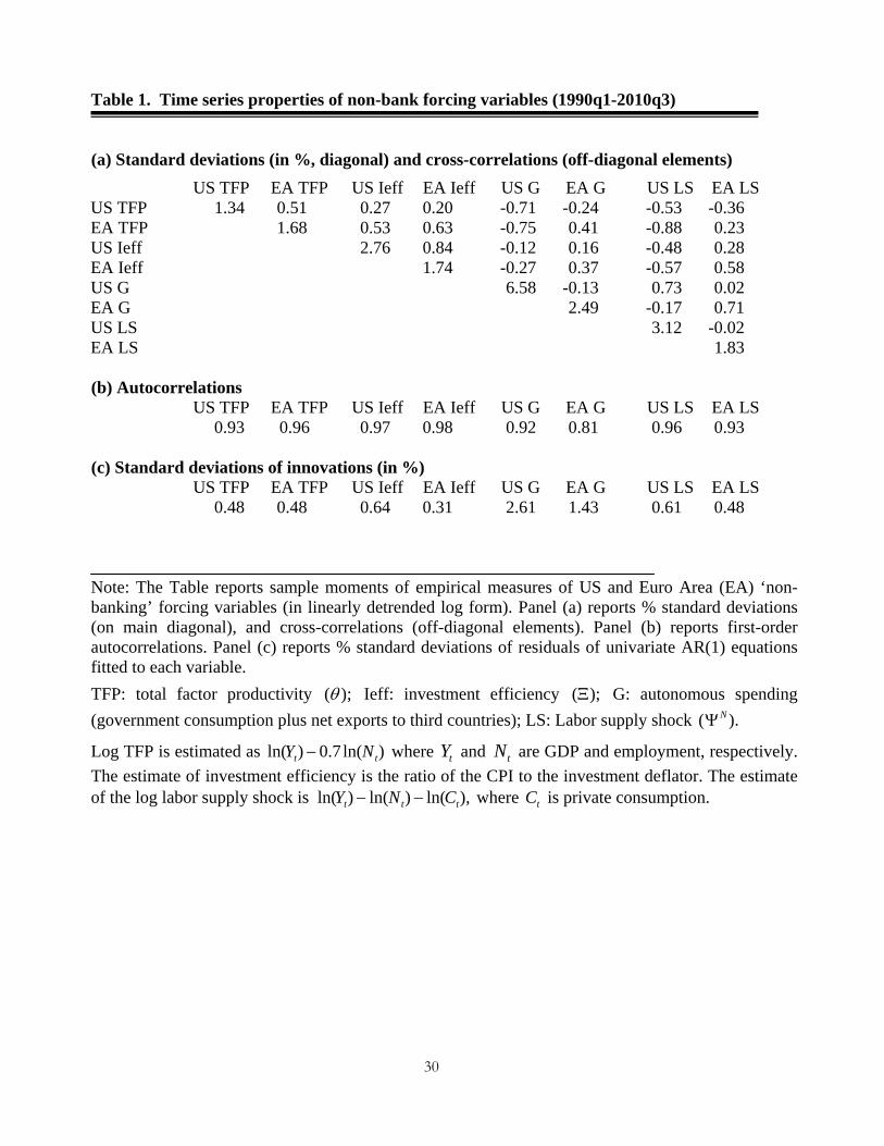
Table 1. Time series properties of non-bank forcing variables (1990q1-2010q3) (a) Standard deviations (in %, diagonal) and cross-correlations (off-diagonal elements)

US TFP EA TFP US Ieff EA Ieff US G EA G US LS EA LS US TFP 1.34 0.51 0.27 0.20 -0.71 -0.24 -0.53 -0.36 EA TFP 1.68 0.53 0.63 -0.75 0.41 -0.88 0.23 US Ieff 2.76 0.84 -0.12 0.16 -0.48 0.28 EA Ieff 1.74 -0.27 0.37 -0.57 0.58 US G 6.58 -0.13 0.73 0.02 EA G 2.49 -0.17 0.71 US LS 3.12 -0.02 EA LS 1.83 (b) Autocorrelations US TFP EA TFP US Ieff EA Ieff US G EA G US LS EA LS

0.93 0.96 0.97 0.98 0.92 0.81 0.96 0.93 (c) Standard deviations of innovations (in %) US TFP EA TFP US Ieff EA Ieff US G EA G US LS EA LS

0.48 0.48 0.64 0.31 2.61 1.43 0.61 0.48 Note: The Table reports sample moments of empirical measures of US and Euro Area (EA) ‘non-banking’ forcing variables (in linearly detrended log form). Panel (a) reports % standard deviations (on main diagonal), and cross-correlations (off-diagonal elements). Panel (b) reports first-order autocorrelations. Panel (c) reports % standard deviations of residuals of univariate AR(1) equations fitted to each variable.

TFP: total factor productivity ( );θ Ieff: investment efficiency ( );Ξ G: autonomous spending (government consumption plus net exports to third countries); LS: Labor supply shock ( ).NΨ

Log TFP is estimated as ln( ) 0.7 ln( )t tY N− where tY and tN are GDP and employment, respectively. The estimate of investment efficiency is the ratio of the CPI to the investment deflator. The estimate of the log labor supply shock is ln( ) ln( ) ln( ),t t tY N C− − where tC is private consumption.

31

Table 2. Historical business cycle statistics US EA Standard deviations (in%) GDP (Y) 1.12 1.14 Consumption 0.92 0.78 Investment 5.10 2.89 Employment 1.16 0.71 Loans 1.61 1.98 Bank capital ratio 0.49 -- Loan rate spread (p.a.) 0.19 0.38 Correlations with domestic GDP Consumption 0.89 0.83 Investment 0.92 0.93 Employment 0.79 0.83 Loans 0.48 0.59 Bank capital ratio 0.19 -0.01 Loan rate spread -0.52 -0.91 Cross-country correlations GDP 0.56 Consumption 0.39 Investment 0.45 Employment 0.53 Loans 0.53 Loan rate spread 0.79 Note: Moments of HP filtered series are shown (GDP, consumption, investment, employment and loans were logged before applying the filter). The bank capital ratio is expressed in fractional units. The loan rate spread is expressed in fractional units per annum. The correlations of the bank capital ratio with domestic GDP reported in the Table are correlations of the US commercial bank capital ratio with US GDP and EA GDP. Sample period: 1990q1-2010q3 (except for EA loan spread: 2003q1-2010q3).

32

Table 3. Prior and posterior parameter distributions for the baseline model ( '' 0)φ > and a model variant without operative bank capital requirement ( '' 0)φ = Baseline model: Model with '' 0 :φ = Prior distribution Posterior distribution Posterior distribution Parameter Mean Std Distrib Mode Mean Std 5% 95% Mode Mean Std (1) (2) (3) (4) (5) (6) (7) (8) (9) (10) (11) Behavioral parameters 4 ''γφ 0.20 0.10 G 0.44 0.44 0.06 0.34 0.54 0.00 0.00 0.00

''ξ 1.00 0.50 G 0.09 0.09 0.01 0.07 0.11 0.08 0.08 0.01 σ 1.00 0.50 G 0.81 0.81 0.05 0.72 0.90 0.57 0.58 0.04

Parameters of banking shocks distributions ( )Std ε Δ 0.50 0.10 IG 0.48 0.51 0.07 0.39 0.64 0.57 0.62 0.10

*( )Std ε Δ 0.50 0.10 IG 1.38 1.41 0.17 1.15 1.71 0.67 0.71 0.09

( )Std γε 0.50 0.10 IG 0.53 0.56 0.07 0.45 0.70 0.46 0.50 0.10 *( , )Corr ε εΔ Δ 0.50 0.10 B 0.34 0.35 0.08 0.23 0.49 0.46 0.45 0.08

ρΔ 0.50 0.10 B 0.59 0.56 0.07 0.44 0.67 0.54 0.52 0.07 *ρΔ 0.50 0.10 B 0.48 0.48 0.06 0.38 0.59 0.91 0.90 0.02

γρ 0.50 0.10 B 0.79 0.78 0.03 0.72 0.83 0.56 0.59 0.14

ϑΔ 0.00 0.10 N 0.10 0.11 0.02 0.07 0.15 0.14 0.14 0.02 γϑ 0.00 0.10 N 0.07 0.06 0.02 0.03 0.10 0.13 0.16 0.12

Standard deviations (%) of measurement errors GDP US 0.79 0.16 IG 0.40 0.40 0.04 0.34 0.48 0.41 0.41 0.05 GDP EA 0.54 0.11 IG 0.30 0.30 0.04 0.25 0.37 0.38 0.39 0.05 C US 0.78 0.16 IG 0.57 0.58 0.06 0.47 0.69 0.43 0.44 0.05 C EA 0.44 0.09 IG 0.37 0.38 0.05 0.29 0.48 0.31 0.33 0.05 I US 3.15 0.63 IG 3.46 3.50 0.35 2.95 4.11 4.05 4.07 0.36 I EA 1.33 0.26 IG 0.95 1.01 0.15 0.78 1.29 1.76 1.77 0.35 N US 0.47 0.09 IG 0.45 0.46 0.05 0.37 0.56 0.47 0.48 0.06 N EA 0.45 0.09 IG 0.28 0.29 0.03 0.23 0.35 0.31 0.31 0.04 Loans US 0.85 0.17 IG 0.87 0.88 0.07 0.76 1.01 0.86 0.88 0.09 Loans EA 1.10 0.22 IG 0.47 0.48 0.05 0.40 0.58 0.45 0.46 0.05 Bank cap. ratio 0.21 0.04 IG 1.31 1.32 0.13 1.12 1.54 0.88 0.88 0.15 Loan rate spread 0.03 0.01 IG 0.02 0.02 0.00 0.02 0.03 0.10 0.10 0.01 Notes: Cols. (1) and (2) shows the means and standard deviations of the prior distribution for model parameters. Col. (3) indicates the distribution function of the prior (B: Beta; G: Gamma; IG: Inverted Gamma; N: Normal). Cols. (4)-(8) show statistics of the posterior parameter distribution, for the baseline model (means, modes, standard deviations, 5th and 95th percentiles). Cols. (9)-(11) show statistics of the posterior parameter distribution for a model variant without an operative bank capital requirement (for that variant, the priors in Cols. (1)-(3) are used, except that ''φ is set at '' 0).φ = Posterior distributions are computed using the Random Walk Metropolis algorithm (250,000 draws of which the first 50,000 were discarded)

33

Table 4. Baseline model: implied business cycle statistics Non- All banking Banking Invest. Loan Required shocks shocks shocks TFP Eff. G LabS Loss Bnk.Cap Data (1) (2) (3) (4) (5) (6) (7) (8) (9) (10) (a) Country ‘Home’ (US) moments Standard deviations (in%) GDP (Y) 1.30 1.20 0.32 0.94 0.14 0.23 0.78 0.28 0.15 1.12 Consumption 1.34 1.21 0.14 0.64 0.10 0.10 0.63 0.12 0.06 0.92 Investment 5.37 3.80 1.81 1.54 2.33 0.41 1.58 1.60 0.84 5.10 Employment 1.16 0.97 0.45 0.49 0.12 0.33 1.09 0.40 0.21 1.16 Loans 1.49 0.95 0.79 0.44 0.92 0.17 0.34 0.77 0.16 1.61 Bank cap ratio 1.36 0.10 0.50 0.07 0.03 0.01 0.04 0.47 0.19 0.49 Loan spread 0.38 0.12 0.36 0.08 0.03 0.02 0.05 0.19 0.29 0.19

Correlations with domestic GDP Consumption 0.76 0.93 -0.87 0.93 0.26 -0.98 0.91 -0.85 -0.92 0.89 Investment 0.61 0.81 0.99 0.93 -0.03 0.12 0.95 0.99 0.99 0.92 Employment 0.79 0.89 0.99 0.90 0.85 0.99 0.99 0.99 0.99 0.79 Loans 0.33 0.45 0.47 0.46 0.80 0.24 0.69 0.46 0.71 0.48 Bank cap ratio 0.04 -0.49 0.84 -0.33 -0.63 -0.36 -0.11 0.93 0.47 0.19 Loan spread -0.02 0.58 -0.82 0.42 0.62 0.65 0.29 -0.94 -0.91 -0.52

(b) Country ‘Foreign’ (EA) moments Standard deviations (in%) GDP (Y) 0.88 0.75 0.35 0.77 0.29 0.14 0.74 0.31 0.15 1.14 Consumption 0.91 0.82 0.16 0.74 0.20 0.08 0.42 0.15 0.06 0.78 Investment 2.52 1.41 1.87 1.57 0.71 0.56 1.56 1.67 0.84 2.89 Employment 0.95 0.77 0.49 0.43 0.42 0.20 1.03 0.44 0.21 0.71 Loans 1.14 0.32 1.00 0.14 0.24 0.15 0.19 0.99 0.12 1.98 Bank cap ratio 1.36 0.10 0.50 0.07 0.03 0.01 0.04 0.47 0.19 -- Loan spread 0.38 0.12 0.36 0.08 0.03 0.02 0.05 0.19 0.29 0.38

Correlations with domestic GDP Consumption 0.46 0.68 -0.92 0.85 -0.96 -0.89 0.92 -0.93 -0.92 0.83 Investment 0.54 0.52 0.99 0.96 -0.50 -0.47 0.91 0.99 0.99 0.93 Employment 0.59 0.56 0.99 0.59 0.99 0.99 0.99 0.99 0.99 0.83 Loans 0.27 0.19 0.65 0.72 0.02 0.14 0.56 0.69 0.80 0.62 Bank cap ratio 0.27 -0.33 0.86 -0.34 -0.28 -0.00 -0.36 0.94 0.49 -0.01 Loan spread -0.18 0.42 -0.81 0.40 0.34 0.29 0.30 -0.95 -0.90 -0.91

(c) Cross-country correlations GDP 0.44 0.44 0.99 -0.06 -0.26 0.43 -0.53 0.99 0.99 0.56 Consumption 0.76 0.91 0.94 0.70 0.72 0.80 0.18 0.93 0.99 0.39 Investment 0.30 0.15 0.99 -0.20 -0.58 -0.16 -0.72 0.99 0.99 0.45 Employment -0.01 -0.31 0.99 -0.91 -0.04 0.47 -0.52 0.99 0.99 0.53 Loans 0.17 -0.73 0.65 -0.56 -0.83 0.25 -0.72 0.65 0.95 0.64 Loan spread 1.00 1.00 1.00 1.00 1.00 1.00 1.00 1.00 1.00 0.79 Note: The Table shows moments of HP filtered model variables, computed at the posterior mode of the estimated parameters. The bank capital ratio is expressed in factional units. The loan rate spread is expressed in fractional units per annum. Other variables are normalized by steady state values. Col. (1) assumes all 11 structural shocks and measurement error. In Cols. (2)-(9), subsets of shocks are assumed in isolation, without measurement error (model not re-estimated). Col. (2): just the ‘non-banking’ shocks,

nbktε ; Col. (3): just banking shocks, .bk

tε Col. (4): just Home and Foreign TFP shocks; Col. (5): just shocks to investment efficiency; Col. (6): just shocks to government purchases; Col.(7): just labor supply shocks; Col.(8): just loan loss shocks; Col. (9): just shock to required bank capital ratio ( )tγ . Col. (10) shows empirical moments (from Table 2).

34

Table 5. Baseline model: dynamic responses to innovations

GDP Consumption Investment Employment Loans Bank Cap. Loan Horizon US EA US EA US EA US EA US EA Ratio Spread (1) (2) (3) (4) (5) (6) (7) (8) (9) (10) (11) (12)

(a) Home country TFP shock (1%) 0 1.63 -0.48 0.92 0.18 2.84 -0.80 0.88 -0.68 0.03 0.00 -1.51 2.60 4 1.15 -0.40 0.85 0.11 1.20 -0.52 0.48 -0.54 -0.41 0.06 -7.54 8.46 20 0.56 -0.15 0.62 -0.01 -0.04 0.12 0.08 -0.18 -1.63 0.34 -7.98 7.85 (b) Home investment efficiency shock (1%) 0 -0.12 0.41 0.01 -0.24 3.33 -1.51 -0.18 0.57 0.36 -0.15 -0.74 0.86 4 0.08 0.13 0.09 -0.17 2.41 -1.27 -0.03 0.25 1.61 -0.58 -2.52 2.56 20 0.33 -0.20 0.24 -0.08 0.39 -0.31 0.12 -0.15 2.94 -1.02 -2.28 2.27 (c) Home government purchases shock (1%) 0 0.06 0.02 -0.03 -0.01 0.03 -0.15 0.09 0.03 -0.00 -0.01 -0.00 0.15 4 0.06 -0.00 -0.02 -0.01 0.03 -0.12 0.08 0.00 -0.02 -0.05 -0.18 0.47 20 0.04 -0.02 -0.01 -0.01 0.01 -0.01 0.05 -0.01 -0.10 -0.06 -0.17 0.28 (d) Home labor supply shock (1%) 0 -0.93 0.19 -0.77 -0.03 -1.96 0.97 -1.31 0.28 -0.07 0.04 0.42 -1.41 4 -0.82 0.24 -0.75 -0.01 -1.16 0.75 -1.09 0.30 -0.01 0.13 3.17 -4.98 20 -0.45 0.09 -0.57 0.07 -0.07 -0.07 -0.53 0.08 1.31 -0.08 3.12 -4.64 (e) Home loan loss shock (1% of steady state GDP) 0 -0.14 -0.16 0.08 0.04 -0.83 -0.87 -0.20 -0.23 -0.52 -0.04 -14.37 6.26 4 -0.09 -0.11 0.03 -0.01 -0.47 -0.48 -0.10 -0.13 -1.23 -0.11 -21.22 8.63 20 0.01 -0.00 -0.00 -0.05 0.06 0.08 0.03 0.02 -1.23 -0.02 -3.28 1.37 (f) Foreign loan loss shock (1% of steady state GDP) 0 -0.12 -0.13 0.04 0.07 -0.70 -0.73 -0.17 -0.19 -0.05 -0.31 -14.62 6.46 4 -0.07 -0.08 -0.01 0.03 -0.36 -0.37 -0.08 -0.10 -0.15 -0.61 -17.31 7.06 20 0.00 0.00 -0.03 -0.00 0.05 0.06 0.02 0.02 -0.09 -0.54 -2.45 1.03 (g) Shock to required bank capital ratio (1 percentage point) 0 -0.21 -0.21 0.08 0.08 -1.17 -1.14 -0.29 -0.28 -0.09 -0.05 1.32 46.98 4 0.05 0.06 -0.03 -0.04 0.33 0.36 0.09 0.10 0.06 0.09 26.68 6.40 20 0.02 0.03 0.02 0.02 0.07 0.06 0.01 0.02 0.33 0.24 7.47 -2.31 Note: The Table shows dynamic responses to exogenous shocks, after 0, 4 and 20 quarters (see left-most column labeled ‘Horizon’), of the variables listed at the top of the Table. The responses are computed at the posterior mode of the estimated parameters. In each case, an isolated innovation is considered, assuming that all other exogenous innovations are zero. Panel (a): 1% innovation to Home TFP ( )θ ; Panel (b): 1% innovation to US investment efficiency ( );Ξ Panel (c): 1% innovation to government purchases ( );G Panel (d): 1% innovation to US labor supply preference parameter ( );NΨ Panel (e): innovation to Home loan loss ( )Δ worth 1% of steady state GDP; Panel (f) innovation to Foreign loan loss *( )Δ worth 1% of steady state GDP; Panel (g) innovation that raises required bank capital ratio ( )γ by 1 percentage point. Cols. (1)-(2): Responses of US and EA GDP; Cols. (3)-(4): US and EA consumption; Cols. (5)-(6): US and EA investment; Cols. (7)-(8): US and EA employment; Cols. (9)-(10): US and EA loans; Col. (11): bank capital ratio; Col. (12): Loan rate spread. Responses of the bank capital ratio are in basis points. Responses of the loan spread are in bp per annum. Other responses are in percentage points of steady state values.

35

Table 6. Model variant without operative bank capital requirement ( '' 0)φ = : implied business cycle statistics Non- All banking Banking Invest. Loan Required shocks shocks shocks TFP Eff. G LabS Loss Bnk.Cap Data (1) (2) (3) (4) (5) (6) (7) (8) (9) (10) (a) Country ‘Home’ (US) moments Standard deviations (in%) GDP (Y) 1.83 1.79 0.01 1.25 0.21 0.23 0.99 0.00 0.00 1.12 Consumption 1.27 1.20 0.06 0.62 0.23 0.15 0.76 0.06 0.00 0.92 Investment 7.52 6.43 0.02 2.79 3.12 0.44 2.66 0.00 0.02 5.10 Employment 1.83 1.77 0.00 0.87 0.22 0.33 1.39 0.00 0.00 1.16 Loans 1.76 1.43 0.60 0.43 1.19 0.16 0.52 0.60 0.00 1.61 Bank cap ratio 1.12 0.52 0.52 0.39 0.16 0.08 0.32 0.52 0.00 0.49 Loan spread 0.38 0.00 0.01 0.00 0.00 0.00 0.00 0.00 0.01 0.19

Correlations with domestic GDP Consumption 0.85 0.92 0.19 0.95 -0.12 -0.95 0.99 0.35 -0.65 0.89 Investment 0.75 0.90 0.83 0.98 0.39 0.49 0.95 0.10 0.99 0.92 Employment 0.91 0.96 0.80 0.99 0.90 0.99 0.99 0.07 0.98 0.79 Loans 0.41 0.52 -0.20 0.68 0.85 0.34 0.72 -0.37 0.75 0.48 Bank cap ratio 0.16 0.36 0.25 0.21 -0.28 0.15 -0.11 0.45 0.78 0.19 Loan spread 0.01 0.87 -0.83 0.74 0.70 0.88 0.67 -0.45 -0.99 -0.52

(b) Country ‘Foreign’ (EA) moments Standard deviations (in%) GDP (Y) 1.31 1.25 0.01 1.09 0.39 0.16 0.89 0.00 0.01 1.14 Consumption 1.10 1.06 0.07 1.04 0.33 0.12 0.59 0.07 0.00 0.78 Investment 3.75 3.34 0.02 3.06 0.82 0.32 2.12 0.00 0.02 2.89 Employment 1.20 1.17 0.00 0.64 0.55 0.22 1.25 0.00 0.00 0.71 Loans 1.35 1.04 0.75 0.96 0.36 0.17 0.69 0.75 0.00 1.98 Bank cap ratio 1.12 0.52 0.52 0.39 0.16 0.08 0.32 0.52 0.00 -- Loan spread 0.38 0.00 0.01 0.00 0.00 0.00 0.00 0.00 0.01 0.38

Correlations with domestic GDP Consumption 0.71 0.77 0.04 0.97 -0.97 -0.92 0.97 0.12 -0.36 0.83 Investment 0.76 0.89 0.91 0.97 0.23 -0.64 0.96 0.18 0.99 0.93 Employment 0.83 0.89 0.87 0.98 0.99 0.99 0.99 0.14 0.98 0.83 Loans 0.43 0.59 -0.24 0.67 0.33 0.29 0.68 -0.60 0.79 0.62 Bank cap ratio 0.35 0.51 -0.10 0.57 0.56 0.52 0.56 -0.26 0.79 -0.01 Loan spread 0.47 0.83 -0.91 0.74 0.85 0.80 0.49 0.26 -0.99 -0.91

(c) Cross-country correlations GDP 0.70 0.75 0.55 0.32 0.27 0.68 -0.17 -0.96 0.99 0.56 Consumption 0.78 0.86 -0.99 0.35 0.73 0.98 -0.18 -0.99 0.94 0.39 Investment 0.58 0.77 0.99 0.44 0.20 -0.59 -0.18 0.99 0.99 0.45 Employment 0.49 0.53 0.99 0.10 0.53 0.72 -0.16 0.99 0.99 0.53 Loans 0.23 0.27 0.33 -0.18 -0.44 -0.16 -0.43 0.33 0.74 0.64 Loan spread 1.00 1.00 1.00 1.00 1.00 1.00 1.00 1.00 1.00 0.79

Note: For the model variant without an operative bank capital requirement ( '' 0),φ = the Table shows moments of HP filtered model variables, computed at the posterior mode of the estimated parameters. The bank capital ratio is expressed in factional units. The loan rate spread is expressed in fractional units per annum. Other variables are normalized by steady state values. Col. (1) assumes all 11 structural shocks and measurement error. In Cols. (2)-(9), subsets of shocks are assumed in isolation, without measurement error (model not re-estimated). Col. (2): just the ‘non-banking’ shocks, nbk

tε ; Col. (3): just banking shocks, .bktε Col. (4): just

Home and Foreign TFP shocks; Col. (5): just shocks to investment efficiency; Col. (6): just shocks to government purchases; Col.(7): just labor supply shocks; Col.(8): just loan loss shocks; Col. (9): just shock to required bank capital ratio ( )tγ . Col. (10) shows empirical moments (from Table 2).

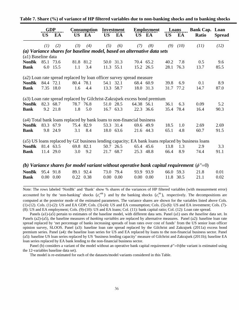
36

Table 7. Share (%) of variance of HP filtered variables due to non-banking shocks and to banking shocks

GDP Consumption Investment Employment Loans Bank Cap. Loan

US EA US EA US EA US EA US EA Ratio Spread (1) (2) (3) (4) (5) (6) (7) (8) (9) (10) (11) (12) (a) Variance shares for baseline model, based on alternative data sets (a1) Baseline data NonBk 85.1 73.6 81.8 81.2 50.0 31.3 70.4 65.2 40.2 7.8 0.5 9.6 Bank 6.0 15.5 1.1 3.4 11.3 55.1 15.2 26.5 28.1 76.3 13.7 85.5 (a2) Loan rate spread replaced by loan officer survey spread measure NonBk 84.4 72.1 80.4 78.1 54.1 32.1 68.4 60.9 39.8 6.9 0.1 8.9 Bank 7.35 18.0 1.6 4.4 13.3 58.7 18.0 31.3 31.7 77.2 14.7 87.0 (a3) Loan rate spread replaced by Gilchrist-Zakrajsek excess bond premium NonBk 82.3 68.7 78.7 76.8 51.0 28.5 64.38 56.1 36.1 6.3 0.09 5.2 Bank 9.2 21.8 1.8 5.0 16.7 63.3 22.3 36.6 35.4 78.4 16.4 90.3 (a4) Total bank loans replaced by bank loans to non-financial business NonBk 83.3 67.9 75.4 82.9 53.3 31.4 69.6 49.9 18.5 1.0 2.69 2.69 Bank 9.8 24.9 3.1 8.4 18.0 63.6 21.6 44.3 65.1 4.8 60.7 91.5 (a5) US loans replaced by GZ business lending capacity; EA bank loans replaced by business loans NonBk 81.4 63.5 69.8 82.1 50.7 26.5 65.4 45.6 13.8 1.3 2.9 3.3 Bank 11.4 29.0 3.0 9.2 21.7 68.7 25.3 48.8 66.4 8.9 74.4 91.1 (b) Variance shares for model variant without operative bank capital requirement ( '' 0)φ = NonBk 95.4 91.8 89.1 92.4 73.0 79.4 93.9 93.9 66.0 59.3 21.8 0.01 Bank 0.00 0.00 0.22 0.38 0.00 0.00 0.00 0.00 11.8 30.5 21.1 0.02

Note: The rows labeled ‘NonBk’ and ‘Bank’ show % shares of the variances of HP filtered variables (with measurement error) accounted for by the ‘non-banking’ shocks ( )nbk

tε and by the banking shocks ( ),bktε respectively. The decompositions are

computed at the posterior mode of the estimated parameters. The variance shares are shown for the variables listed above Cols. (1)-(12). Cols. (1)-(2): US and EA GDP; Cols. (3)-(4): US and EA consumption; Cols. (5)-(6): US and EA investment; Cols. (7)-(8): US and EA employment; Cols. (9)-(10): US and EA loans; Col. (11): bank capital ratio; Col. (12): Loan rate spread. Panels (a1)-(a5) pertain to estimates of the baseline model, with different data sets. Panel (a1) uses the baseline data set. In Panels (a2)-(a5), the baseline measures of banking variables are replaced by alternative measures. Panel (a2): baseline loan rate spread replaced by ‘net percentage of banks increasing spreads of loan rates over cost of funds’ from the US senior loan officer opinion survey, SLOOS. Panel (a3): baseline loan rate spread replaced by the Gilchrist and Zakrajsek (2011a) excess bond premium series. Panel (a4): the baseline loan series for US and EA replaced by loans to the non-financial business sector. Panel (a5): baseline US loan series replaced by US ‘business lending capacity’ measure of Gilchrist and Zakrajsek (2011b); baseline EA loan series replaced by EA bank lending to the non-financial business sector. Panel (b) considers a variant of the model without an operative bank capital requirement '' 0φ = (the variant is estimated using the 12-variables baseline data set). The model is re-estimated for each of the datasets/model variants considered in this Table.

37

Figure 1. Time series used in estimation

Note: The Figure shows the time series used in estimation. Bank capital ratio and loan spread (p.a.) are demeaned. Other variables are logged and detrended. Shaded areas indicate US recessions (NBER dates).

38

Figure 2. US and EA loan rate spreads

Note: Loan spreads (p.a.) are not demeaned. Shaded areas: US recessions (NBER dates). Figure 3a. US bank capital, loan spread and SLOOS spread measure

Note: The solid line shows the demeaned bank capital ratio; the dashed line shows the demeaned loan spread; the dotted line shows a survey-based measure of the net percentage of banks increasing spreads (from Survey of Senior Loan Officers Opinion Survey, SLOOS). Shaded areas: US recessions (NBER dates). Figure 3b. US bank capital and Gilchrist-Zakrajsek (2011a) bond premium

Note: The solid line shows the demeaned bank capital ratio; the dashed line shows the demeaned excess bond premium of Gilchrist and Zakrajsek (2011a). Shaded areas: US recessions (NBER dates).

39

Figure 4. Historical decompositions (baseline estimation)

40

Figure 4—ctd.

Note: The Figure shows the historical contributions of banking shocks (thin solid lines), US non-banking shocks (dashed-dotted lines), EA non-banking shocks (dashed lines) to historical series (thick solid lines). The decompositions are computed at the posterior mode of the estimated parameters. The historical bank capital ratio and loan rate spread series (p.a.) are demeaned, the other historical series are linearly detrended in log form. Shaded areas: US recessions (NBER dates).

41

Figure 5a. US commercial banks: total loans, business loans and business lending capacity

Note: The solid line shows total US bank credit (baseline measure); dashed line: business lending; dashed-dotted line: US business lending capacity (Gilchrist and Zakrajsek (2011b). All series are linearly detrended in log form. Shaded areas: US recessions (NBER dates). Figure 5b. EA banks: total loans and business loans

Note: The solid line shows total EA bank credit (baseline measure); dashed line: loans to non-financial corporations. Both series are linearly detrended in log form. Shaded areas: US recessions (NBER dates).