Global alignments - review

Take two sequences: X[j] and Y[j]

The best alignment for X[1…i] and Y[1…j] is called M[i, j]

Initiation: M[0,0]=0

Apply the equation Find the alignment with

backtracing

M[i, j] = M[i, j-1] – 2

M[i-1, j] – 2

M[i-1, j-1] ± 1

max

6543210

76543210

AGCGGAG

0-AGTGAG-

X[j]

Y[i]

2

Algorithm time/space complexity - Big-O Notation

a simple description of complexity:– constant O(1), linear O(n), quadratic

O(n2), cubic O(n3)... asymptotic upper bound read: “order of”

f n=O g nsimple ,e.g.n2

iff. ∃x0,c

∀x≥x0

f x ≤cg x

x0=17

f xln x

2⋅ln x

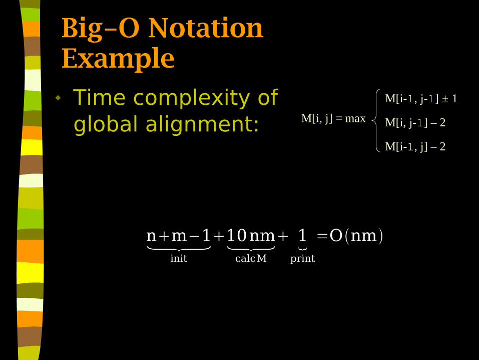
Big-O NotationExample

Time complexity of global alignment:

nm−1init

10nmcalcM

1print

=Onm

M[i, j] = M[i, j-1] – 2

M[i-1, j] – 2

M[i-1, j-1] ± 1

max

Global alignment – linear space

We need O(nm) time, but only O(m) space– how?

problem with backtracking

M[i, j] = M[i, j-1] – 2

M[i-1, j] – 2

M[i-1, j-1] ± 1

max

Global alignment – linear space, recursion

n/2

k1

k2

j j'i

i'

LSpacei , i ' , j , j ':

LSpacei ,n2−1, j ,k1

LSpacei ,n21, j ,k2

space complexity: O(m)

Global alignment – linear space, algorithm

LSpacei , i ' , j , j ':

return if area i , i ' , j , j 'empty

h:= i '−i2

calc.MusingOmmemoryplusfindpathLh

crossingtherowhLSpacei ,h−1,k1 , j 'printLh

LSpacei ,h1,k2 , j '

time complexity: ∑i=0

log2n nm2i ≤ 2nm

h=n/2

k1

k2

j j'i

i'

Lh

Alignments:Local alignment

Local alignment:Smith-Waterman algorithm

What’s local?– Allow only parts of the sequence to

match

– Locally maximal: can not make it better by trimming/extending the alignment

Seq X:

Seq Y:

Local alignment

Why local?– Parts of sequence diverge faster

evolutionary pressure does not put constraints on the whole sequence

– Proteins have modular constructionsharing domains between sequences

Seq X:

Seq Y:

seq X:

seq Y:

seq X:

seq Y:

Domains - exampleImmunoglobulin domain

Global → local alignment

Take the global equation

Look at the result of the global alignment

q

e

s

-

euqes-

CAGCACTTGGATTCTCG-CA-C-----GATTCGT-G

a) global align

b) retrieve the result

c) sum score along the result

align.pos.

sum

Local alignment – breaking the alignment A recipe

– Just don’t let the score go below 0

– Start the new alignment when it happens

– Where is the result in the matrix?

Before: After:

sum

align.pos.

q

e

s

0-

euqes-

q

e

0s

0-

euqes-

sum

align.pos.

sum

align.pos.

Local alignment – the equation

Init the boundaries with 0’s Run the algorithm Read the maximal value

from anywhere in the matrix

Find the result with backtracking

M[i, j] =M[i, j-1] – g

M[i-1, j] – g

M[i-1, j-1] + score(X[i],Y[j])

max

0Great contribution to science!

q

e

s

-

euqes-

Finding second best alignment We can find the best local alignment in

the sequence But where is the second best one?

…

1613A

1815G

1618201714A

15171916G

141618A

…

…AGA…

A clump

Best alignment

Scoring:1 for match-2 for a gap

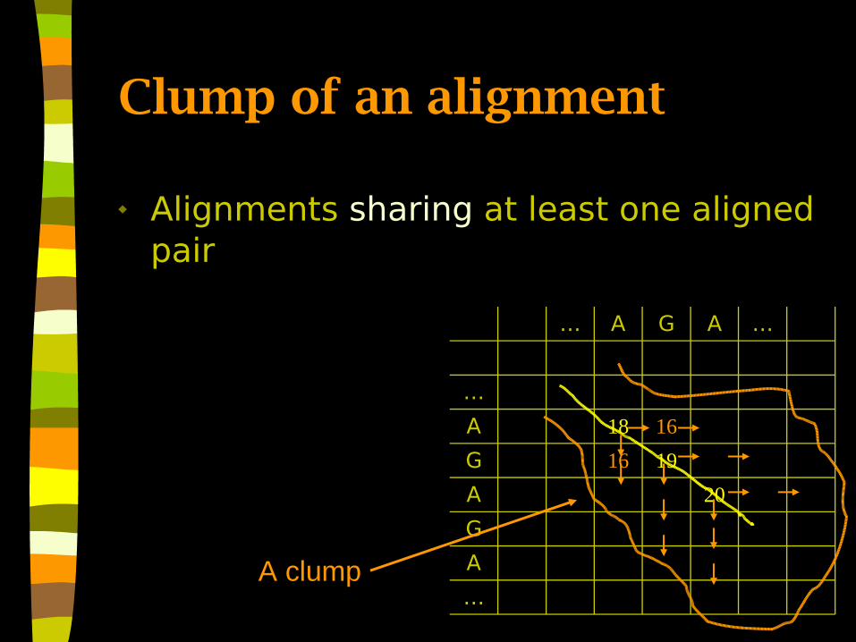
Clump of an alignment

Alignments sharing at least one aligned pair

…

A

G

20A

1916G

1618A

…

…AGA…

A clump

Clumpsge

ne Y

gene X

Finding second best alignment Don’t let any matched pair to

contribute to the next alignment

1…

130A

02G

10001A

0000G

100A

…

…AGA…

Recalculate the clump

“Clear” the best alignment

Extraction of local alignments – Waterman-Eggert algorithm

1. Repeata. Calc M without taking cells into

account

b. Retrieve the highest scoring alignment

c. Set it’s trace to

Clumpsge

ne Y

gene X

Clumpsge

ne Y

gene X

Low complexity regions Local composition

bias– Replication slippage:

e.g. triplet repeats Results in spurious

hits– Breaks down statistical

models– Different proteins

reported as hits due to similar composition

– Up to ¼ of the sequence can be biased

Huntington’s disease

– Huntingtin gene of unknown (!) function

– Repeats #: 6-35: normal; 36-120: disease

Pitfalls of alignments

Alignment is not a reconstruction of the evolution(common ancestor is extinct by the time of alignment)

Pitfalls of alignments

Matches to the same fragment

Arbitrary poor alignment regions

seq X:

seq Y:

Summary1. Global

a.k.a. Needleman-Wunsch algorithm

2. Global-local3. Local

a.k.a. Smith-Waterman algorithm

4. Many local alignmentsa.k.a. Waterman-Eggert algorithm

What’s the number of steps in these algorithms? How much memory is used?

seq X:

seq Y:

seq X:

seq Y:

seq X:

seq Y:

seq X:

seq Y:

Amino acid substitution matrices

Percent Accepted Mutations distance and matrices

Accepted by natural selection– not lethal

– not silent

Def.: S1 and S

2 are PAM 1 distant if

on avg. there was one mutation per 100 aa

Q.: If the seqs are PAM 8 distant, how many residues may be diffent?

PAM matrix Created from “easy”alignments

– pairwise

– gapless

– 85% id

f proline − frequencyof occurenceof proline

f proline, valine − frequencyof substitution

prolinewith valine,forPAM1

i.e. f a ,b=∑aligns

count a ,b

∑aligns

∑c,d!=a ,b

count c,d

M − symmetricmatr ix ,

i.e. M=[f a ,a f a,b

f b,a f b,b]

PAM matrix How to calculte M for PAM 2

distance?– Take more distant seqs

– or extrapolate...

M2=[f a,a f a,b

f b,a f b,b]2

=[f a,af a ,af a,bf b,a f a,af a,bf a ,bf b,b

⋯ ⋯ ]

PAM log odds matrix Making of the PAM N matrix

Why log? Mutations and chance:

• More freq: PAM N[a,b] > 0

• Less freq: PAM N[a,b] < 0

By chance alone

PAMN [a,b] = log2

f aMN[a ,b]f af b

= log2MN[a ,b]f bodds

logodds

observed

PAM 250 matrix

BLOSUM matrix

BLOcks SUbstitution Matrix Based on gapless alignments More often used than PAM

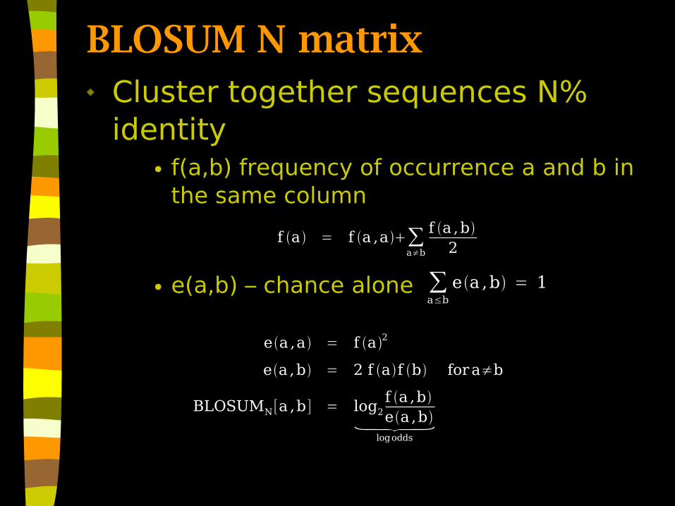
BLOSUM N matrix Cluster together sequences N%

identity• f(a,b) frequency of occurrence a and b in

the same column

• e(a,b) – chance alone

f a = f a ,a∑a≠b

f a,b2

ea,a = f a2

ea,b = 2 f af b fora≠b

BLOSUMN[a ,b] = log2f a ,bea,b

logodds

∑a≤b

ea ,b = 1

BLOSUM 62 matrix# BLOSUM Clustered Scoring Matrix in 1/2 Bit Units# Blocks Database = /data/blocks_5.0/blocks.dat# Cluster Percentage: >= 62# Entropy = 0.6979, Expected = -0.5209 A R N D C Q E G H I L K M F P S T W Y VA 4 -1 -2 -2 0 -1 -1 0 -2 -1 -1 -1 -1 -2 -1 1 0 -3 -2 0R -1 5 0 -2 -3 1 0 -2 0 -3 -2 2 -1 -3 -2 -1 -1 -3 -2 -3N -2 0 6 1 -3 0 0 0 1 -3 -3 0 -2 -3 -2 1 0 -4 -2 -3D -2 -2 1 6 -3 0 2 -1 -1 -3 -4 -1 -3 -3 -1 0 -1 -4 -3 -3C 0 -3 -3 -3 9 -3 -4 -3 -3 -1 -1 -3 -1 -2 -3 -1 -1 -2 -2 -1Q -1 1 0 0 -3 5 2 -2 0 -3 -2 1 0 -3 -1 0 -1 -2 -1 -2E -1 0 0 2 -4 2 5 -2 0 -3 -3 1 -2 -3 -1 0 -1 -3 -2 -2G 0 -2 0 -1 -3 -2 -2 6 -2 -4 -4 -2 -3 -3 -2 0 -2 -2 -3 -3H -2 0 1 -1 -3 0 0 -2 8 -3 -3 -1 -2 -1 -2 -1 -2 -2 2 -3I -1 -3 -3 -3 -1 -3 -3 -4 -3 4 2 -3 1 0 -3 -2 -1 -3 -1 3L -1 -2 -3 -4 -1 -2 -3 -4 -3 2 4 -2 2 0 -3 -2 -1 -2 -1 1K -1 2 0 -1 -3 1 1 -2 -1 -3 -2 5 -1 -3 -1 0 -1 -3 -2 -2M -1 -1 -2 -3 -1 0 -2 -3 -2 1 2 -1 5 0 -2 -1 -1 -1 -1 1F -2 -3 -3 -3 -2 -3 -3 -3 -1 0 0 -3 0 6 -4 -2 -2 1 3 -1P -1 -2 -2 -1 -3 -1 -1 -2 -2 -3 -3 -1 -2 -4 7 -1 -1 -4 -3 -2S 1 -1 1 0 -1 0 0 0 -1 -2 -2 0 -1 -2 -1 4 1 -3 -2 -2T 0 -1 0 -1 -1 -1 -1 -2 -2 -1 -1 -1 -1 -2 -1 1 5 -2 -2 0W -3 -3 -4 -4 -2 -2 -3 -2 -2 -3 -2 -3 -1 1 -4 -3 -2 11 2 -3Y -2 -2 -2 -3 -2 -1 -2 -3 2 -1 -1 -2 -1 3 -3 -2 -2 2 7 -1V 0 -3 -3 -3 -1 -2 -2 -3 -3 3 1 -2 1 -1 -2 -2 0 -3 -1 4

PAM vs BLOSUM

PAM is extrapolation from closely related seqs

We are interested more distant relationships

http://www.ncbi.nih.gov/Education/BLASTinfo/Scoring2.html