GLIMS Regional Center ‘Antarctic Peninsula’

GLIMS RC 18 procedures and guidelines for glacier analysis

Frank Rau, Steffen Vogt, Fabian Mauz & Florian König

Institut für Physische Geographie, Freiburg (Germany)

(Version 2.0) 2004-12-15

This document describes a comprehensive workflow for deriving GLIMS glacier information with a combined approach using predominantly ERDAS Imagine and GLIMSview in addition to ArcInfo / ArcView. The following stepwise algorithm is focussing on the derivation of the relevant parameters and the required spatial data (polygons / segments) from VNIR and SWIR satellite data (LANDSAT & ASTER). A detailed description and discussion of a test data set from Horseshoe Island (Marguerite Bay) is included to stimulate further discussions. GLIMS RC 18 procedures and guidelines for glacier analysis: 1. GIA - ASTER co-registration

Results obtained from GPS accuracy tests and further analysis of imagery indicate that the differences between the GIA Landsat mosaic rigorously re-projected to UTM (WGS 84) and UTM-projected ASTER imagery are fairly small and that both datasets can be combined consistently. To perform the co-registration in accordance to the guidelines of the GLIMS Regional Center ‘Antarctic Peninsula’ the GIA dataset will be selected as geodetic image-map base due to its overall high accuracy. ASTER images (or higher products such as single-pass mosaics) are co-registered to corresponding GIA subsets of the matching UTM zone by applying a first order polynomial model based on GCPs identified in both datasets. In order to preserve the geometric image quality, a ‘cubic convolution’ resampling can be applied, although classification purposes might indicate the selection of a ‘nearest neighbour’ method as the better choice. Our experiences indicate that typical Root Mean Square (RMS) errors in the order of 10 to 20 meters, i.e. approximately one ASTER pixel, can be achieved. Use as a minimum the VNIR and SWIR data (combined as layer stack in one file; resampled to 15 m pixel spacing).

2. ERDAS Imagine: Display corrected geo-referenced image file (UTM, WGS84) in a viewer and open a new vector layer (Arc coverage) with double precision, enable editing mode and set snapping environment (e.g. node snap to 1-2 pixel, arc snap to 2-4 pixel) and weed distance (e.g. 0.25 – 0.5 pixel).

GLIMS Regional Center ‘Antarctic Peninsula’ Glacier analysis - procedures and guidelines

2

Fig. 1: General workflow for glacier analysis as proposed by the RC Antarctic Peninsula

3. Digitise entire catchment boundary of an individual glacier as line features in the current coverage. Digitise always all line segments of the entire glacier boundary in a single consistent order (Important for subsequently assigning the segment attributes).

• Use optionally additional data sources (e.g. maps, DEMs, field data, aerial photography) to facilitate the best as possible identification of the boundary.

• If catchment boundaries from neighbouring glaciers are already existent, extract relevant segments and paste them on the current coverage.

• For high altitude areas with extensive plateau glaciers, extract relevant catchment boundary segments from DEM-analysis and paste them on the current coverage For details: http://intranet/projekte/antarktis/catchment_doku/basin_description.htm

4. Save and review the digitised catchment boundary:

• Is it hydrologically / glaciologically correct? • Does the current catchment boundary fit to the neighbouring glacier catchments?

GLIMS Regional Center ‘Antarctic Peninsula’ Glacier analysis - procedures and guidelines

3

• Do the digitised segments form a closed polygon including the ice-front? • Are the nodes of the various segments connected?

5. ArcInfo: Build the polygon topology with the commands BUILD or CLEAN:

BUILD <cover> {POLY | LINE | POINT | NODE | ANNO.<subclass>} CLEAN <in_cover> {out_cover} {dangle_length} {fuzzy_tolerance} {POLY | LINE}

6. ERDAS Imagine: Check the resulting polygon draped on the satellite image.

7. Generate glacier catchment AOI:

• Open vector tool palette. • Select entire vector polygon. • AOI-Menu: Copy selection to AOI. • Save AOI.

8. Glacier mapping using different approaches such as ratios, NDSI or multi-spectral classification:

• Optional: Generation of a cloud mask. • Optional: Generation of a water mask (be careful if there is brash ice near the

glacier font!). • Calculate band ratios and/or NDSI and adjust correspondent threshold for

separating snow and ice versus other:

o TM4 / TM5 resp. AST3 / AST4 o TM3 / TM5 resp. AST2 / AST4 o Normalized Difference Snow Index (NDSI)

(TM2 - TM5) / (TM2 + TM5) resp. (AST1 – AST4) / (AST1 + AST4)

For further details: http://www.geo.unizh.ch/~kaeaeb/glims/algor.html

• Apply generated cloud and / or water masks. • Reclassify the ratio/NDSI image applying the glacier catchment AOI (snow & ice =1;

other = 0) using the ERDAS model maker: EITHER 0 IF ( $n1_input-image < threshold_value ) OR 1 OTHERWISE

• Analyse results in viewer and compare the different approaches. In particular, evaluate areas of cast shadows, cloud cover and cloud shadows, and frontal areas neighbouring brash-ice covered sea. It might be necessary to apply more sophisticated approaches to map the different parts of larger glaciers (e.g. combined application of different threshold values; DEM analysis, etc.).

• Apply median filter if required (kernel 3 x 3) to remove single out- or inlying pixels. • Eliminate small patches of ice and snow, which are not connected to the glacier:

o Open INTERPRETER => GIS ANALYSIS. o Use module CLUMP (8 connecting neighbours) to identify clumps, which are

contiguous groups of pixels => this routine assigns an individual identifier to all pixels of each polygon. Check raster attributes and assign colours to identify the resulting polygons (use option EDIT => ADD AREA COLUMN).

o Use module SIEVE to eliminate clumps of data values (which have been identified with the Clump function) that are smaller than a minimum size you specify (in general, everything which is smaller than the glacier..)

GLIMS Regional Center ‘Antarctic Peninsula’ Glacier analysis - procedures and guidelines

4

• Analyse results in viewer => the resulting image contains only the polygon of the investigated glacier.

• Vectorise glacier polygon: o Open new vector layer (Arc coverage) with double precision, enable editing

mode and set snapping environment (e.g. node snap to 0.5 - 1 pixel, arc snap to 1-2 pixel) and disable weed distance => these settings result in reasonable (and reproducible..) vectorisation of the polygons taking the pixel centers as vertices.

o Open vector tool palette. o Open vector tools and set REGION GROWING PROPERTIES (8 pixel

neighbourhood mode, disable geographic constraints, Spectral Euclidian Distance = 0 (!), include island polygons (Options)).

o Use REGION GROWING TOOL to vectorise the glacier polygon. o Save and review resulting glacier boundary and the inlying island polygons. o Create attributes using the vector attribute editor.

9. ArcInfo: Build the polygon topology with the commands BUILD or CLEAN:

BUILD <cover> {POLY | LINE | POINT | NODE | ANNO.<subclass>} CLEAN <in_cover> {out_cover} {dangle_length} {fuzzy_tolerance} {POLY | LINE}

10. Clip the resulting glacier polygon to the catchment polygon to remove outlying boundary segments (guarantees that the glacier area is smaller or equal to the catchment area and facilitates a subsequent creation of the topology with neighbouring glaciers):

CLIP <in_cover> <clip_cover> <out_cover> {POLY | LINE | POINT | NET | LINK | RAW} {fuzzy_tolerance}

11. ERDAS Imagine: Open viewer and display the resulting polygon. As a consequence of the previous CLIP-operation, the outer glacier boundary line might be fragmented into numerous individual segments. Unsplit the boundary segments:

• Enable editing mode. • Select all segments using the box selector from the vector tool palette or the line

attribute table. • Select the VECTOR => JOIN option from the viewers menu bar to merge

neighbouring segments (JOIN combines two arcs that share a node, if they are the only two lines sharing that node; the combined lines cannot have more than 500 points).

• Rebuild the polygon topology in ArcInfo with the commands BUILD or CLEAN.

12. Check catchment and glacier polygons draped on the satellite image (particularly after the usage of the CLEAN command!). Check or create attributes using the vector attribute editor.

13. Prepare data for further analysis:

• Export satellite data (3 bands e.g. 3,2,1 or 4,3,2; entire image or only parts of it) as GeoTIFF => image.tif (Attention: 16-bit images cannot be exported to TIFF => convert to 8-bit data using INTERPRETER => Utilities => RESCALE.

• Export Arc coverages to glacier_shapefile.shp and catchment_shapefile.shp. • Drape shapefiles in an ERDAS viewer over the original raster image. • Open vector info and add coverage projection corresponding to the original image’s

projection. • Save and close all shapefiles.

GLIMS Regional Center ‘Antarctic Peninsula’ Glacier analysis - procedures and guidelines

5

• Open all shapefiles in ArcGIS. • Reproject shapefiles using the ArcView projection utility (Slooooow!) or ArcInfo to

geographic coordinates (WGS84) =>shapefile_geo.shp. • Compare original and reprojected shapefiles in an ERDAS viewer draped on the

original raster image.

14. GLIMSview: Open new session in GLIMSview:

• Use image.tif as image file (Note: It is possible to load ERDAS Imgine’s *.img files directly into GLIMSview, however it might be handier to work with the converted TIFF-files).

• Make sure to use standardised line set (RC18 specific?). • Import shapefile_geo.shp using the option PROJECT => IMPORT SHAPEFILE.

When a generic shapefile is imported into GLIMSview, its shape objects are added to the current project's vector dataset with default configurations => normally (..) arcs appear as green lines; points are not visible (as they are no arcs…), but they are present in the current vector layer (try to drag a selection box over the point to select it!).

• Save current session frequently - there is no autosave function! • Split lines into specific segments and assign attributes from the configuration

window. Left and right refers to the direction of digitising (when digitising in a clockwise order, the glacier should be on the right side….). Edit line types and/or create new line types if required (particularly to reflect spatial accuracy of digitised line segments and to attribute material/feature types.

• Create and edit the glacier ID using the information from the IPG glacier inventory e.g. via the web interface at

http://www.geographie.uni-freiburg.de/ipg/forschung/glims_rc/glacierdb_index.htm • Assign the glacier ID to the segments (set lines). • Add ancillary data in appropriate database fields. • Export data using PROJECT => INGEST => EXPORT. • Check resulting shapefiles in ArcView and / or ERDAS Imagine. • Check resulting XML-file in a text- or XML-editor.

15. Send the data to the GLIMS database via the submission interface at

http://extranet.nsidc.org/nasa/daac/glims/submission.html

Concluding remarks: While most parts (1 – 13) of the outlined workflow can be realised without further

problems instantaneously when appropriate imagery becomes available, the final steps (14) of attributing the line segments and preparing the transfer data using the GLIMSview program are more intricate as the current program version 1.0 (release date:2004-12-05) is still affected by a number of software-inherent bugs. In addition, some glacier parameters are not yet precisely defined and, therefore, the guidelines for analysts require a further refinement. Important information can be found at: GLIMSview http://www.glims.org/glimsview/

On-line documentation on the use of GLIMSview http://www.glims.org/glimsview/doc/GLIMSView_UsersGuide.html

GLIMS Regional Center ‘Antarctic Peninsula’ Glacier analysis - procedures and guidelines

6

GLIMSview bug report and enhancement requests http://www.glims.org/glimsview/bug_report/glimsview_1.0_bugs.html

GLIMS Data Dictionary (version 2003-07-02) http://www.glims.org/MapsAndDocs/DB/data_dictionary_20030703.html

Brief Description of GLIMS Database Tables (version 2002-09-30) http://www.glims.org/MapsAndDocs/DB/GLIMSTabledefs20020930.html

List of valid values for various database parameters (version 2003-10-09) http://www.glims.org/MapsAndDocs/datatransfer/valids.txt

GLIMS Data Transfer Specification (version 2003-10-09) http://www.glims.org/MapsAndDocs/datatransfer/data_transfer_specification.html

A few people working with GLIMSView have noticed that as a project gets large, the

potential for abnormal program termination increases and at the least, its responsiveness slows down. In case you are using GLIMSView and haven't figured out the maximum practical size of a project on your machine, it seems to be around 500 MB for a laptop with 1 GB of memory (comment from Bruce Raup, 15 March 2005)

Proposed convention for glacier polygons in

GLIMS (see discussion in GLIMS mail-list, February 2005): o Glacier outline polygons are to be closed o Internal rock boundary polygons are to be

closed o Glacier and rock polygons can be composed

of different segments that carry different attributes, specifying what materials or features are on the "left" and "right" sides.

o Glacier polygons will be stored in the database such that their vertices will be in counterclockwise order, as you look down from above.

o Internal rock polygons will be stored in the database such that their vertices will be in clockwise order, as you look down from above.

o Given a rock-ice boundary, ice will always be on the left, and rock will always be on the right (Debris cover doesn't count as "rock").

This convention is in agreement with Oracle standards (spatial database extension) and the Open GIS GML specification. For the analysts, the following implications are improtant: o The RCs and Stewards do not need to worry about putting the segments or vertices in the

proper order, since the GLIMS ingest software does this already. Specifically, it strings segments of the same type (e.g. "glac_bound" or "intrnl_rock") with the same glacier ID together in the right order, reversing the direction of segments as needed (which might have been digitized in the other direction compared to the rest of the polygon), and detects gaps or open polygons.

o What RCs and Stewards do need to pay attention to is the definition of "left" and "right". It doesn't matter what direction a segment is digitized in, but the attributes of what materials are on the "left" and "right" must be assigned according to this definition.

Fig. 2: Convention for glacier polygons inGLIMS (source: Bruce Raup, 2005).

GLIMS Regional Center ‘Antarctic Peninsula’ Glacier analysis - procedures and guidelines

7

GLIMS RC 18 Test Data Set: Shoesmith Glacier (Horseshoe Island, Marguerite Bay) The Shoesmith Glacier on Horseshoe Island (Marguerite Bay, Antarctic Peninsula) was selected for a first test of analysing and preparing GLIMS-related glacier data. As this particular glacier is a rather small one, the analysis and its results provide an example of a (typical) GLIMS analysis session. Hereby, we were confronted with a variety problems and open questions, which have to be discussed and solved in order to provide in the near future consistent and reliable guidelines for glacier analysis. The present data set of the Shoesmith Glacier should therefore be regarded as a starting point for a further discussion. Data analysis was realised by a combined approach of using ERDAS Imagine 8.5, ArcView 3.2 and GLIMSview 0.99. The field definitions for the analysis session and the resulting 4 mandatory shapefiles were extracted from ‘GLIMS Antarctic Peninsula – Regional Center (AP-RC): Glacier analysis submissions to NSIDC database guide’ compiled by R Jaña on basis of the documents available on the GLIMS web pages. The shapefiles were generated using GLIMSview 0.99 and are not corrected (e.g. N/S bug in the segments IDs).

Fig. 3: The GLIMSview desktop during the analysis session ‘Shoesmith Glacier’.

GLIMS Regional Center ‘Antarctic Peninsula’ Glacier analysis - procedures and guidelines

8

In the following section, a brief description of the assigned valids and attributes is provided. 1 session shapefile

• The information was added directly in the XML-file, as the required fields are not completely represented in the GLIMSview configuration menu.

• Institutional information was set to RC 18 (Antarctic Peninsula, IPG Freiburg). • Further information on image processing, additional sources (in this case the

Horseshoe Island map (FIDS/BAS) and the correspondent geographic region was provided in <ProcDesc> and <DataSrc>.

2 glaciers shapefile

• Glacier name and coordinates refer to the IPG glacier inventory ‘Antarctic Peninsula’ and were extracted from Marguerite Bay record (marguerite_geo.shp). The local glacier ID corresponds to the current version (November 2003).

• The glacier name was checked by analysing HATTERLEY-SMITH (1991). • The classification scheme corresponds to the IPG glacier classification. • Snowline altitude was estimated from map source. • Glacier length was determined along the centreline. • Glacier area determined by thresholding ASTER 3/4 ratio image using the catchment

polygon to mask out the neighboured glaciers. • Glacier width was measured (roughly) up-glacier of the divergence of the two ice

tongues. • The Id of the glacier in the exported shapefile is erroneous due to a bug in the

GLIMSview export routine (southern latitudes are interpreted as northern ones!). The XML-file contains the correct values.

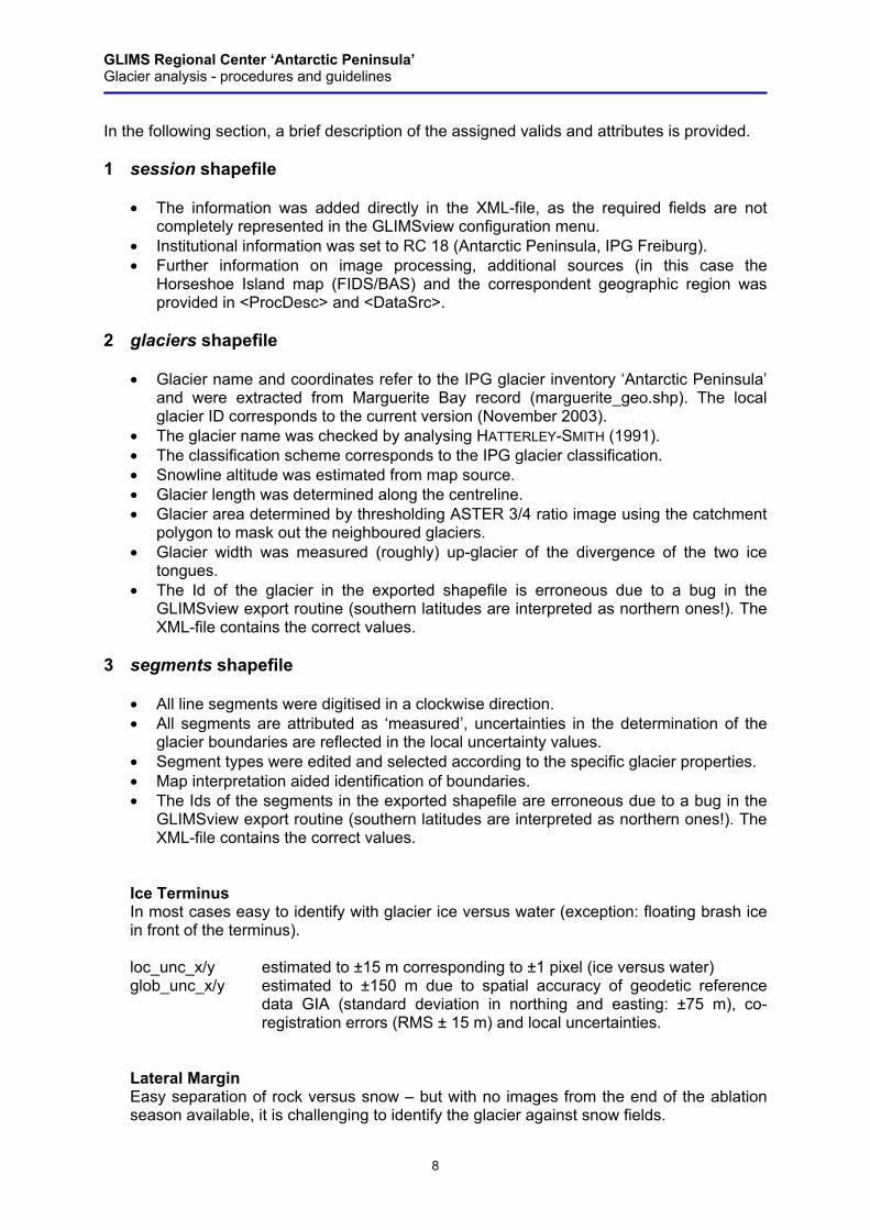
3 segments shapefile

• All line segments were digitised in a clockwise direction. • All segments are attributed as ‘measured’, uncertainties in the determination of the

glacier boundaries are reflected in the local uncertainty values. • Segment types were edited and selected according to the specific glacier properties. • Map interpretation aided identification of boundaries. • The Ids of the segments in the exported shapefile are erroneous due to a bug in the

GLIMSview export routine (southern latitudes are interpreted as northern ones!). The XML-file contains the correct values.

Ice Terminus In most cases easy to identify with glacier ice versus water (exception: floating brash ice in front of the terminus). loc_unc_x/y estimated to ±15 m corresponding to ±1 pixel (ice versus water) glob_unc_x/y estimated to ±150 m due to spatial accuracy of geodetic reference

data GIA (standard deviation in northing and easting: ±75 m), co-registration errors (RMS ± 15 m) and local uncertainties.

Lateral Margin Easy separation of rock versus snow – but with no images from the end of the ablation season available, it is challenging to identify the glacier against snow fields.

GLIMS Regional Center ‘Antarctic Peninsula’ Glacier analysis - procedures and guidelines

9

loc_unc_x/y estimated to ±30 m corresponding to 2 pixel. glob_unc_x/y estimated to ±150 m due to spatial accuracy of geodetic reference

data GIA (standard deviation in northing and easting: ±75 m), co-registration errors (RMS ± 15 m) and local uncertainties.

Head boundary Easy separation of rock versus snow – but with no images from the end of the ablation season available, it is challenging to identify the glacier against snow fields. Difficult identification of ice divides. As line segment separates ice/rock and ice/ice, neither left material nor left features were assigned. loc_unc_x/y estimated to ± 30 m corresponding to ±2 pixel. glob_unc_x/y estimated to ± 150 m due to spatial accuracy of geodetic reference

data GIA (standard deviation in northing and easting: ±75 m), co-registration errors (RMS ± 15 m) and local uncertainties.

Internal Rock No segment label seems to be appropriate. No right (inner) feature was assigned, as no feature class seems to be appropriate (mountain?). loc_unc_x/y ± 30 (the center line does not represent a physical feature of a glacier

and digitised more or less arbitrarily by the analysts). glob_unc_x/y ± 150 m (see above). Center Line No left/right material or feature was assigned. loc_unc_x/y ±0 (the center line does not represent a physical feature of a glacier

and digitised more or less arbitrarily by the analysts). glob_unc_x/y ±150 m (see above). Snow Line Rough estimate of the snowline position => although there are snow-free patches up-glacier, the current snow line represents the upper limits of the area which is almost completely snow free. loc_unc_x/y ±100 m. glob_unc_x/y ±250 m (see above). Basin Boundary Entire catchment area (not only glacier surface) as line segments forming a closed polygon including the ice front => equal or larger than glacier! No left/right material/feature was assigned. As it is difficult (or impossible..) to edit overlapping lines in the current GLIMSview version, all segments of the basin boundary were edited in a individual GLIMSview session and subsequently copied into the final XML-file (including the correspondent line definition). loc_unc_x/y ±30 m. glob_unc_x/y ±150 m (see above).

GLIMS Regional Center ‘Antarctic Peninsula’ Glacier analysis - procedures and guidelines

10

4 image shapefile In general, it is not always clear if this section refers to the original, unaltered satellite image or to the pre-processed, value-added image product which was used for analysis. In the present analysis session, we decided to provide in this shapefile basically the information of the processed satellite image (<ImageID> and coordinates; further information on image processing is provided in the session shapefile) with additional basic information on the original satellite image file.

• The information was compiled using the meta-information extracted from the original HDF ASTER file and from the ASTER scene database at the GLIMS interactive map web page (http://www.glims.org/astermap.html).

• The information was added directly in the XML-file, as the required fields are not completely represented in the GLIMSview configuration menu.

• The (global) uncertainties values (<CenterLonUnc> and <CenterLatUnc>) refer to the processed image refererenced to the GIA Landsat mosaic. The values were estimated to ±100 m in agreement with the IPG accuracy assessment report (accuracy of GIA and RMS error of coregistration).

• As the center coordinates evidently are directly extracted from the analysed image file by the GLIMSview program, these were replaced and set to the values from the HDF meta information.

• The projection was set to UTM Zone 19 South WGS84.

Contact: Frank Rau Department of Physical Geography University of Freiburg Werderring 4 D-79085 Freiburg - Germany phone: ++49 (0)761 203 3550 fax: ++49 (0)761 203 3596 e-mail: frank.rau@geographie.uni-freiburg.de http://www.geographie.uni-freiburg.de/ipg/ http://www.geographie.uni-freiburg.de/ipg/forschung/ap3/antarctica/