1

GIS AND SPATIAL DATA ANALYSIS: CONVERGING PERSPECTIVES Michael F. Goodchild1 and Robert P. Haining2 1. INTRODUCTION We take as our starting point the state of geographic information systems (GIS) and spatial data analysis 50 years ago when regional science emerged as a new field of enquiry. In the late 1950s and 1960s advances in computing technology were making possible forms of automated cartography that in due course would lead to the development of GIS. Although few would have imagined at that time that the complex graphic content of maps was amenable to processing by number-crunching computers, and that any purpose could be served by doing so, the development of scanners and plotters in the 1960s, along with rapid advances in software, began to open exciting possibilities, even at that very early stage in the development of computing (for histories of early GIS see Foresman, 1998; Maguire, Goodchild, and Rhind, 1991). At the same time pioneering work was taking place in the fields of mathematics and statistics that would be fundamental to the development of spatial data analysis. The seminal paper by Whittle (1954) extended autoregressive models, fundamental in analysing variation in time series (see for example, Kendall, 1976), to spatial data. This group of spatially autoregressive models was amongst the first to appear in the statistics literature for formally representing spatial variation. At least for some types of data, it now became possible to go beyond simply testing for spatial autocorrelation. The earliest statistics (Geary, 1954; Krishna Iyer, 1949; Moran 1948, 1950) tested the null hypothesis of no spatial autocorrelation (no spatial structure) against a non-specific alternative hypothesis. With Whittle's paper it now became possible, at least for regular lattice data, to specify the form of the alternative hypothesis (that is, to specify a formal representation of certain types of spatial structure), test for model significance, and assess goodness of fit to the data. More or less simultaneously with these developments in England, Matheron in France and his school in the mining industry were developing the method of "kriging" after the South African D.G. Krige (Matheron, 1963). This work extended Wiener-Kolmogorov stochastic-process prediction theory to the case of spatial processes defined on continuous geographic space. This work was undertaken to meet the very practical needs of the mining industry in predicting yields from mining on the basis of scattered (opportunistic) sampling. In due course this developed into the field of geostatistics. The third area that was to become one of the main cornerstones of spatial statistics was point process theory. By the 1950s many distance-based and quadrat-based statistics had

1 National Center for Geographic Information and Analysis, and Department of Geography, University of California, Santa Barbara, CA 93106-4060, USA. Phone +1 805 893 8049. FAX +1 805 893 3146. Email good@geog.ucsb.edu 2 Department of Geography, University of Cambridge, Downing Site, Cambridge CB2 3EN, England. Phone +44 (0)1223 333394. Fax +44 (0)1223 333392. Email rph26@cam.ac.uk

2

been developed to test for spatial randomness in a point pattern with applications in forestry and ecology. Work by Greig-Smith (1952) extended quadrat-count statistics to examine several scales of pattern simultaneously. However as yet there was no equivalent development in point process theory to correspond to Whittle's in the area of lattice data. This paper discusses some of the key developments in these areas and the evolution of geographic information science as a unified field that draws upon GIS and the methods of spatial statistics as an essential theoretical underpinning to spatial data analysis. The growth of any science depends on several conditions being met. First, there must be good-quality data available. Second, there must be well-formulated hypotheses that can be formalised, mathematically, so that they can be subject to empirical testing. Third, there must be a rigorous methodology that enables the analyst to draw valid inferences and conclusions from the data in relation to the questions asked. This includes the ability to formulate models that can then be used to test hypotheses on parameters of interest. The final condition is the availability of a technology that permits research to be undertaken practically and to acceptable standards of precision. The evolution of geographic information science (GIScience; Duckham, Goodchild and Worboys, 2003; Goodchild, 1992) owes much to developments in GIS and the field of spatial data analysis. Research into GIS has advanced our technical ability to handle spatially referenced data. In addition it has stimulated reflection on the relationship between what might be loosely termed "geographic reality" and the conceptualization and representation of that reality in finite digital forms, that is, as countable numbers of points, lines and areas in two-dimensional space. Spatial data analysis is concerned with that branch of data analysis where the geographical referencing of objects contains important information. In many areas of data collection, especially in some areas of experimental science, the indexes that distinguish different cases can be exchanged without any loss of information. All the information relevant to understanding the variation in the data set is contained in the observations and no relevant information is contained in the indexing. In the case of spatial data the indexing (by location and time) may contain crucial information. A definition of spatial analysis (of which spatial data analysis is one element) is that it represents a collection of techniques and models that explicitly use the spatial referencing of each data case. Spatial analysis needs to make assumptions about or draw on data describing spatial relationships or spatial interactions between cases. The results of any analysis will not be the same under re-arrangements of the spatial distribution of values or reconfiguration of the spatial structure (Chorley, 1972; Haining 1994). GIS and spatial data analysis come into contact, so to speak, at the spatial data matrix. At a conceptual level, this matrix consists of rows and columns where rows refer to cases and columns refer to the attributes measured at each of the cases, and the last columns provide the spatial referencing. At the simplest level, there might be two last columns containing a pair of coordinates: latitude and longitude, or x and y in some projected coordinate system. But today database technology allows a single conceptual column to contain a complex representation of the case's spatial geometry or shape.

3

This conceptual matrix is but a slice through a larger cube where the other axis is time. At a practical level, the spatial data matrix is the repository of the data collected by the researcher. In practical terms the structure and content of the matrix is the end product of processes of conceptualisation and representation by which some segment of geographical reality is captured. It is in one sense the output of a process of digitally capturing the world. In another sense, the matrix is the starting point or input for the spatial data analyst. Those principally concerned with data analysis need to give careful consideration to how well the data matrix captures the geographic reality underlying the problem and the implications (for interpreting findings) of representational choices. The question of what is missing from the representation – the uncertainty that the representation leaves in the mind of its users about the world being represented (Zhang and Goodchild, 2002) – may be as important as the content in some applications. By the same token those principally concerned with the digital representation of geographical spaces need to be aware of the power of statistical methodology to reveal useful data insights and understandings if data are made available in appropriate forms and subject to appropriate methods of analysis. This paper identifies some of the important developments in GIS and spatial data analysis since the early 1950s. The two started out as rather separate areas of research and application but have grown closer together. It is at least arguable that they meet in the field of GIScience, with each supporting and adding value to the other. In Section 2 we provide a historical perspective of developments over the past fifty years. In Section 3 we reflect on current challenges and speculate about the future. Finally, in Section 4 we comment on the potential for convergence under the rubric of GIScience 2. A CRITICAL RETROSPECTIVE 2.1 GIS 2.1.1 Early motivations The early growth of GIS occurred in several essentially disparate areas, and it was not until the 1980s that a semblance of consensus began to emerge. Perhaps the most important of the motivations for GIS were: • The practical difficulty and tedium of obtaining accurate measurements from maps,

and the simplicity of obtaining such measurements from a digital representation. Specifically, measurement of area became a major issue in conducting inventories of land, and led the Government of Canada to make a major investment in the Canada Geographic Information System beginning in the mid 1960s (Tomlinson, Calkins, and Marble, 1976).

• The need to integrate data about multiple types of features (census tracts, traffic

analysis zones, streets, households, places of work, etc.), and the relationships

4

between them, in large projects such as the Chicago Area Transportation Studies of the 1960s.

• The practical problem of editing maps during the cartographic production process,

leading to the development of the first computerized map-editing systems, again in the 1960s.

• The need to integrate multiple layers of information in assessing the ecological

impacts of development projects, resulting in efforts in the early 1970s to computerize McHarg's overlay method (McHarg, 1992).

• The problems faced by the Bureau of the Census in managing large numbers of

census returns, and assigning them correctly to reporting zones such as census tracts. By the early 1970s the research community was beginning to see the benefits of integrated software for handling geographic information. As with any other information type, there are substantial economies of scale to be realized once the foundation for handling geographic information is built, since new functions and capabilities can be added quickly and with minimal programming effort. The first commercially viable GIS appeared in the early 1980s, as the advent of the minicomputer made it possible to acquire sufficient dedicated computing power within the budget of a government department or firm, and as relational database management software obviated the need to construct elaborate data-handling functions from first principles. The economies of scale that underlie the viability of commercial GIS also impose another important constraint: the need to address the requirements of many applications simultaneously, and to devote the greatest attention to the largest segments of the market. Spatial data analysis may be the most sophisticated and compelling of GIS applications, but it is by no means the most significant commercially (Longley et al., 2001). Instead, the modal applications tend to be driven by the much simpler needs of query and inventory. In utilities management, for example, which has become among the most lucrative of applications, the primary value of GIS lies in its ability to track the locations and status of installations, rather than to conduct sophisticated analysis and modeling. Applications of GIS to scientific research have always had to compete with other demands on the attention of system developers, and while this might be seen as beneficial, in the sense that spatial data analysis does not have to pay the full cost of GIS development, it is also undoubtedly detrimental. 2.1.2 Early mis-steps From the point of view of spatial data analysis, it is easy to identify several early decisions in the design of GIS that in hindsight turn out to have been misguided, or at least counter-productive. In the spirit of a critical review, then, this section examines some of those mis-steps.

5

First, GIS designs typically measure the locations of points on the Earth's surface in absolute terms, relative to the Earth's geodetic frame, in other words the Equator and the Greenwich Meridian. This makes good sense if one assumes that it is possible to know absolute location perfectly, and that as measuring instruments improve the accuracy of positions in the database will be enhanced accordingly. Two fundamental principles work against this position. First, it is impossible to measure location on the Earth's surface perfectly; and relative locations can be measured much more accurately than absolute locations. Because of the wobbling of the Earth's axis, uncertainty about the precise form of the Earth, and inaccuracies in measuring instruments it is possible to measure absolute location to no better than about 5m. But it is possible to measure relative locations much more accurately; the distance between two points 10km apart is readily measured to the nearest cm, using standard instruments. In hindsight, then, it would have been much more appropriate to have designed GIS databases to record relative locations, and to have derived absolute locations on the fly when necessary (Goodchild, 2002). Second, and following directly from the previous point, the GIS industry has been very slow to incorporate methods for dealing with the uncertainty associated with all aspects of GIS. The real world is infinitely complex, and it follows that it is impossible to create a perfect representation of it. Zhang and Goodchild (2002) review two decades of research into the measurement, characterization, modeling, and propagation of uncertainty. Yet very little of this research has been incorporated into commercial products, in part because there has been little pressure from users, and in part because uncertainty represents something of an Achilles' heel for GIS, a problem that if fully recognized might bring down the entire house of cards (Goodchild, 1998). Third, the relational database management systems (RDBMS) introduced in the early 1980s provided an excellent solution to a pressing problem, the need to separate GIS software from database management, but the solution was only partial. In the hybrid systems that flourished from 1980 to 1995 the attributes of features were stored in the RDBMS, but the shapes and locations of features had to be stored in a separate, custom-built database that was unable to make use of standard database-management software. The reason was very simple: the shapes of features could not be defined in the simple tabular structure required by an RDBMS. It was not until the late 1990s that the widespread adoption of object-oriented database management systems in preference to RDBMS finally overcame this problem, and allowed all of the data to be addressed through a separate, generic database-management system. 2.1.3 Two world views Many of the roots of GIS lie in mapping, and the metaphor of the map still guides GIS design and application. But many of the applications of interest to regional scientists and other researchers are not map-like, and in such cases the metaphor tends to constrain thinking. GIS works well when applied to static data, and less well when called upon to analyze time series, detailed data on movement, or transactions. It works well for two-dimensional data, and less well when the third spatial dimension is important. We expect

6

maps to provide a complete coverage of an area, and GIS technology has not been adapted to deal with cases where substantial quantities of data are missing. The emphasis in GIS on knowledge of the absolute positions of cases and their precise geometry is appropriate for mapping, but for many applications in the social sciences it is relative position or situation that is important. Many theories about the operation of social or economic processes in space are invariant under relocation, reflection, or rotation, though not under change in relative position. Many methods of spatial statistics or spatial analysis are similarly invariant under a range of spatial transformations, and require only knowledge of a matrix of spatial interactions between cases, not their exact coordinates. Conveniently, the literatures of both spatial interaction and social networks use the symbol W for the interaction matrix. In the spatial case, the elements of W might be set equal to a decreasing function of distance, or to a length of common boundary, or might be set to 1 if the cases share a common boundary, and 0 otherwise. As an expression of spatial relationships the W matrix is compact and convenient. The GIS, with its vastly more complex apparatus for representing spatial properties, is useful for calculating the elements of W from distances or adjacencies, and for displaying the results of analysis in map form. However the actual analysis can occur in a separate set of software that needs to recognize only the square W matrix of interactions and the normally rectangular spatial data matrix discussed above in Section 1. In recent years much progress has been made using this concept of coupling analysis software with GIS. In essence, the GIS and the W matrix reflect two distinct world views, one providing a complete, continuous representation of spatial variation, and the other providing a much more abstract, discrete representation. In this second world view the concern for precise representation of absolute position that has characterised the development of GIS is important only for data preparation and the mapping of results. 2.1.4 Infrastructure for data sharing The Internet explosion of the late 1990s produced a substantial change of perspective in GIS, and redirected much of the development effort in the field. In the U.S., the Federal government has traditionally been the primary source of geographic information, and under U.S. law such data has the characteristics of a public good, freely sharable without copyright restriction. Since 1995, the GIS community has made a massive investment in infrastructure to support the rapid and easy sharing of geographic information, and today there are on the order of petabytes of geographic information readily available, free, on numerous Web sites (see, for example, the Alexandria Digital Library, http://www.alexandria.ucsb.edu). New standards have been developed by the U.S. Federal Geographic Data Committee (http://www.fgdc.gov) and the Open GIS Consortium (http://www.opengis.org) for data formats, for the description of data (metadata), and for communication. New technologies have been developed to allow GIS users to interact with remote Web sites transparently through client software, removing any need to transform data in response to differences in format, projection, or geodetic datum.

7

A parallel effort was under way much earlier in the social sciences, through organizations such as the UK's Essex Data Archive, or the University of Michigan's Inter-university Consortium for Political and Social Research. Sophisticated methods have been developed for describing matrices of data, many of which include spatial information. The Data Documentation Initiative (DDI; http://www.icpsr.umich.edu/DDI/) is an international effort to define a metadata standard for social data, and efforts are now under way to integrate it with the metadata standards for GIS data, to allow researchers to search for both types simultaneously. 2.1.5 The current state of GIS Today, GIS is a multi-billion-dollar industry, with billions being spent annually on data acquisition and dissemination, software development, and applications. It has penetrated virtually all disciplines that deal in any way with the surface or near-surface of the Earth, from atmospheric science through oceanography to criminology and history. Tens of thousands take courses in GIS each year, and millions are exposed to GIS through such services as Mapquest (http://www.mapquest.com). Millions more make use of the Global Positioning System and simple devices to navigate. The object-oriented approach now dominates GIS data modeling. Its first principle is that every feature on the Earth's surface is an instance of a class, and its second is that classes can be specializations of more general classes. The authors, for example, are instances of the class male human beings, which is a specialization of the more general class human beings. In turn human beings can be thought of as part of a hierarchy of increasing generality: mammals, vertebrates, animals, and organisms in that order. Specialized classes inherit all of the properties of more general classes, and add special properties of their own. GIS permits a vast array of operations based on this approach to representation. Most published methods of spatial analysis can be found implemented in the standard products of commercial GIS vendors, or in the extensions to those products that are offered by third parties. A variety of GIS products and extensions are also available as open software or freeware, through academic and other organizations and communities. The GIS industry has recently adopted component-based approaches to software, by breaking what were previously monolithic packages into aggregations of re-usable components. This has enormous advantages in the integration of GIS with other forms of software that use the same standards, particularly packages for statistical analysis (Ungerer and Goodchild, 2002). Much progress has been made in recent years in supporting the representation of variation in space-time, and in three spatial dimensions. But in one respect the shift to industry-standard object-oriented modeling has failed to address several very important forms of geographic data. While the concept of discrete objects is clearly appropriate for human beings, vehicles, buildings, and manufactured objects, it is much less compatible with many phenomena in the geographic world that are fundamentally continuous: rivers,

8

roads, or terrain are obvious examples. In social science, we tend to think of population density as a continously varying field, expressed mathematically as a function of location, and similarly many other social variables are better conceived as fields (Angel and Hyman, 1976). Fields can be represented in GIS, but only by first attributing their variation to a collection of discrete objects, such as sample points, or stretches of street between adjacent intersections, or reporting zones. In the last case the consequences of attributing continous variation to arbitrary chunks of space are well documented as the modifiable areal unit problem (Openshaw, 1983). As long as object-orientation remains the dominant way of thinking about data in the computing industry and in GIS, social scientists will have to wrestle with the artifacts created by representing continuous variation in this way. 2.2 Progress in spatial data analysis The review of progress in spatial data analysis since the early 1950s is divided into two parts. First we review developments in the statistical theory for analysing spatial data. This is followed by a review of new techniques and methods. One aspect of the progress made has been in the emergence of new fields of application, which we review in Section 3 in the context of the future development of spatial data analysis. 2.2.1 Development of theory An overview of the theory for analysing spatial data in the late 1960s and early 1970s would have shown that developments up to then had been rather patchy. There were no books which brought together advances in the field and which tried to present them within a broader theoretical framework. There was no field of spatial statistics as such, although the term spatial analysis had entered the geographical literature (e.g., Berry and Marble, 1968). The closest to such an overview text was Matern's 1960 monograph Spatial Variation (Matern, 1986). This situation stood in stark contrast to the analysis of time-series data where several major theoretical texts existed (e.g., Anderson, 1971; Grenander and Rosenblatt, 1957; Kendall, 1976; Wold, 1954), as well as econometrics texts that dealt with the analysis of economic time series (e.g., Johnston, 1963; Malinvaud, 1970). In most texts and monographs, if the analysis of spatial data was mentioned the coverage was usually sparse with the exception of Bartlett's 1955 monograph Stochastic Processes (Bartlett, 1955). It was Bartlett's early work that was to provide the basis for a new class of spatial models for area data that were developed in the seminal paper by Besag, which appeared in 1974. Models were developed that satisfied a two-dimensional version of the Markov property – the property that underlay many of the important models for representing temporal variation. As a result of Besag's paper it was possible to specify a general class of spatial models for discrete- and continuous-valued variables defined in two-dimensional space. We illustrate the difference between Whittle's and Besag's classes of models using the case of observations (z(1),….,z(T)) drawn from a normal distribution, generalizing the discussion to the case of an irregular areal system (like census tracts in a city). The

9

spatial Markov property underlying Besag's models generalizes the (first order) Markov property in time-series modeling. The Markov property in time (t) states that only the most recent past determines the conditional probability of the present or: Prob{Z(t) = z(t) | Z(1) = z(1),......., Z(t-1) = z(t-1)} =

Prob{Z(t) = z(t) | Z(t-1) = z(t-1)} (2.1)

where Prob{ } denotes probability. Time has a natural ordering. The analog to (2.1) for spatial data is based on defining a graph structure on the set of spatial units. For each area (or site) a set of neighbors is defined that may be, for example, all areas which share a common boundary with it or whose centroids lie within a given distance of the area's centroid. So the analog to (2.1) is: Prob{Z(i) = z(i) | {Z(j) = z(j)}, j ∈ D, j ≠ i} = Prob{Z(i) = z(i) | {Z(j) = z(j)}, j ∈ N(i)}

(2.2) where D denotes the set of all areas (or sites) in the study region and N(i) denotes the set of neighbors of site i. In spatial analysis this has been called the conditional approach to specifying random field models for regional data. Equation (2.2) and higher-order generalizations provide the natural basis for building spatial models that satisfy a spatial form of the Markov property (Haining 2003). A multivariate normal spatial model satisfying the first order Markov property can be written as follows (Besag, 1974; Cressie, 1991, p.407):

E[Z(i)=z(i) | {Z(j)=z(j)}j∈N(i)}] = µ(i) + Σj∈N(i) k(i,j) [Z(j) - µ(j)] i = 1,..,n and (2.3)

Var[Z(i)=z(i) | {Z(j)=z(j)}j∈N(i)}] = σ(i)2 i = 1,..,n where k(i,i) = 0 and k(i,j) = 0 unless j∈N(i). This is called the autonormal or conditional autoregressive model (CAR model). Unconditional properties of the model are, using matrix notation:

E[Z] = µ and Cov[(Z - µ),(Z - µ)T] = (I - K)-1 M. (2.4)

where E[ ] denotes expected value and Cov[ ] denotes the covariance. K is the n by n matrix {k(i,j)} and µ = (µ(1),..,µ(n))T. K is specified exogenously. M is a diagonal matrix where m(i,i) = σ(i)2. Because (I - K)-1 M is a covariance matrix, it must be symmetric and positive definite. It follows that k(i,j) σ(j)2 = k(j,i) σ(i)2. Note that if the conditional variances are all equal then k(i,j) must be the same as k(j,i). If the analyst of regional data does not attach importance to satisfying a Markov property (see for example Haining, 2003 for a discussion of this issue) then another option is available called the simultaneous approach to random-field model specification. It is this approach which Whittle developed in his 1954 paper, and it can be readily generalized to

10

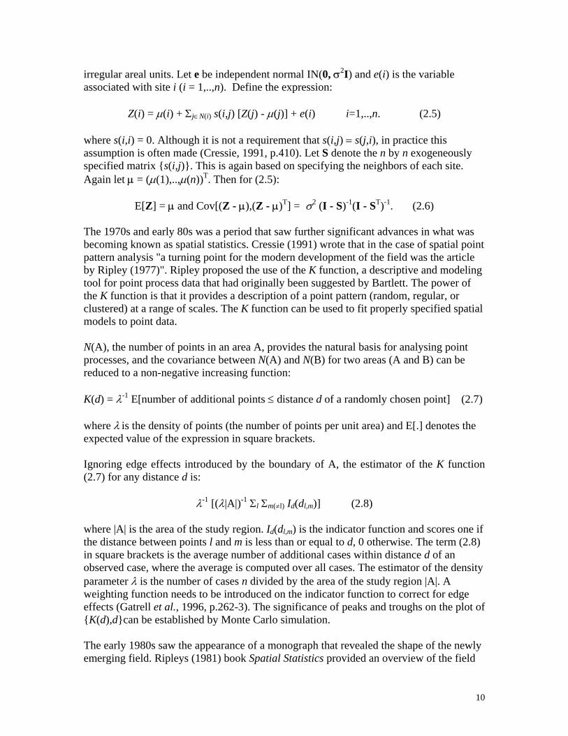
irregular areal units. Let e be independent normal IN(0, σ2I) and e(i) is the variable associated with site i (i = 1,..,n). Define the expression:

Z(i) = µ(i) + Σj∈N(i) s(i,j) [Z(j) - µ(j)] + e(i) i=1,..,n. (2.5) where s(i,i) = 0. Although it is not a requirement that s(i,j) = s(j,i), in practice this assumption is often made (Cressie, 1991, p.410). Let S denote the n by n exogeneously specified matrix {s(i,j)}. This is again based on specifying the neighbors of each site. Again let µ = (µ(1),..,µ(n))T. Then for (2.5):

E[Z] = µ and Cov[(Z - µ),(Z - µ)T] = σ2 (I - S)-1(I - ST)-1. (2.6)

The 1970s and early 80s was a period that saw further significant advances in what was becoming known as spatial statistics. Cressie (1991) wrote that in the case of spatial point pattern analysis "a turning point for the modern development of the field was the article by Ripley (1977)". Ripley proposed the use of the K function, a descriptive and modeling tool for point process data that had originally been suggested by Bartlett. The power of the K function is that it provides a description of a point pattern (random, regular, or clustered) at a range of scales. The K function can be used to fit properly specified spatial models to point data. N(A), the number of points in an area A, provides the natural basis for analysing point processes, and the covariance between N(A) and N(B) for two areas (A and B) can be reduced to a non-negative increasing function: K(d) = λ-1 E[number of additional points ≤ distance d of a randomly chosen point] (2.7) where λ is the density of points (the number of points per unit area) and E[.] denotes the expected value of the expression in square brackets. Ignoring edge effects introduced by the boundary of A, the estimator of the K function (2.7) for any distance d is:

λ-1 [(λ|A|)-1 Σl Σm(≠l) Id(dl,m)] (2.8) where |A| is the area of the study region. Id(dl,m) is the indicator function and scores one if the distance between points l and m is less than or equal to d, 0 otherwise. The term (2.8) in square brackets is the average number of additional cases within distance d of an observed case, where the average is computed over all cases. The estimator of the density parameter λ is the number of cases n divided by the area of the study region |A|. A weighting function needs to be introduced on the indicator function to correct for edge effects (Gatrell et al., 1996, p.262-3). The significance of peaks and troughs on the plot of {K(d),d}can be established by Monte Carlo simulation. The early 1980s saw the appearance of a monograph that revealed the shape of the newly emerging field. Ripleys (1981) book Spatial Statistics provided an overview of the field

11

which included advances in geostatistics. The treatment of geostatistics was included in a chapter on spatial smoothing and spatial interpolation. The importance of this area and the wider significance of Matheron's work beyond the interests of geologists and mining engineers became clear as the field of automated mapping itself began to expand. Another significant monograph at this time was Diggle's (1983) book on point pattern analysis. This linked the K function for describing point pattern structure with models for representing point pattern variation, allowing it to be used to test specific spatial hypotheses. Stoyan, Kendall, and Mecke's (1987) monograph dealt with point processes and stochastic geometry. 1991 saw the publication of Cressie's 900-page work Statistics for Spatial Data – the last time a statistician has provided an overview of the whole field. His text includes methods and models for analysing geostatistical data, lattice data (e.g., including the models of Whittle and Besag), point, and object pattern data. 2.2.2 Development of specific techniques. As noted in Section 1, amongst the earliest spatial analysis techniques were those developed for testing for spatial autocorrelation on regular lattices. For regional science dealing usually with data on irregular areal units this meant the tests were of limited value. Cliff and Ord (1973, 1981) pioneered the development of tests for spatial autocorrelation on irregular areal units, generalizing the earlier tests and examining in detail the associated inference theory. In many areas of non-experimental (or observational) science data have higher levels of uncertainty associated with their measurement than in the case of experimental science. Cressie (1984) introduced techniques for resistant spatial analysis in geostatistics, that is techniques that were more robust (than traditional methods) to data errors and outliers. He also developed methods that could be used to highlight possible errors in spatial data sets. Haining (1990) extended several of Cressie's methods to area data. Many of the early methods of point pattern analysis were limited in the extent to which they could be applied because the underlying space across which events might occur are heterogeneous (or inhomogeneous). Many of the early methods were developed in ecology to study plant distributions across a study area. But to study clustering of disease cases, for example, or offense patterns it is necessary to allow for inhomogeneity in the distribution of the population at risk. Diggle and Chetwynd (1991) used K functions to develop a test for the clustering of cases in an inhomogeneous point pattern. It is a test of the hypothesis of random labeling of (disease) cases in a spatially distributed population. Many of the techniques of spatial analysis have emphasized the average properties present in spatial data. The tests for clustering or spatial autocorrelation described above provide evidence relating to what are termed whole-map properties. In the 1990s, there has been interest in developing localized tests that recognize the heterogeneity of map properties across the study area. In addition to tests for clustering (a whole-map property) that can test the hypothesis as to whether cases of a disease tend to be found together, tests to detect the presence of (localized) clusters are needed. Tests for the presence of

12

clusters may give evidence of where local concentrations are to be found which in turn can be used to focus effort on the extent to which local conditions might be responsible for the raised occurrence. Testing for clusters (see for example, Besag and Newell, 1991; Openshaw et al., 1987; Kulldorff and Nagarwalla, 1995) raise problems such as pre-selection bias and the effects of multiple testing which need to be handled in order to construct a reliable inference theory. Other localized testing procedures include Anselin's (1995) local indicators of spatial association, or LISAs, that test for localized structures of spatial autocorrelation. These numerical methods have been complemented by the development of visualization methods for spatial data (see Haining 2003, for a review). The interaction of scientific visualization methods with advances in automated cartography and GIS has been one of the dynamic areas of spatial analysis in the 1990s (MacEacheren and Monmonier, 1992). The challenge has been to move away from seeing maps purely as end products of a program of research and hence only used to display findings. This requires the integration of automated mapping within the wider analysis agenda of exploring data, suggesting hypotheses and also lines for further enquiry. Mapping is a fundamental element within the scientific visualization of spatial data. 3. CURRENT CHALLENGES AND FUTURE DIRECTIONS 3.1 In GIS 3.1.1 Representations and data sources Despite the limitations and false starts identified in Section 2.1, GIS today represents a solid basis for spatial data analysis. The basic products of the vendors provide a range of techniques for analysis and visualization in addition to the essential housekeeping functions of transformation, projection change, and resampling. Additional analysis techniques are often added through extensions written in scripting languages, and increasingly in languages such as Visual Basic for Applications, frequently by third parties. Various strategies of coupling are also used, to link the GIS with more specialized code for specific applications. Over time the GIS research community has come to focus more and more of its efforts on issues of representation – that is, on the fundamental task of representing the real geographic world in the binary alphabet of the digital computer. Research has focused on the representation of time, which turns out to be far more complex than the simple addition of a third (or fourth) dimension to the two (or three) of spatial representations. Peuquet (2002) provides an analysis of the philosophical and conceptual underpinnings of the problem, and Langran (1992) presents a more practical perspective, while Frank, Raper, and Cheylan (2001) address the issues of reporting zone boundaries that shift through time. Other research has focused on the representation of objects whose boundaries are uncertain (Burrough and Frank, 1996), a common issue in environmental data though perhaps less so in social data.

13

However the problem of time is clearly more than a simple issue of representation. The entire apparatus of Census data collection has traditionally approached time through decennial snapshots, changing reporting zone boundaries in each cycle and creating difficult issues for anyone wishing to analyze Census data in longitudinal series. Not only is there very little available in the way of spatiotemporal data, but our analytic apparatus and theoretical frameworks are similarly limited. The arrival of large quantities of tracking data in recent years, through the use of GPS attached to sample vehicles and individuals, is likely to stimulate renewed interest in this neglected area of both GIS and spatial data analysis. Other new data sources are becoming available through the deployment of high-resolution imaging systems on satellites. It is now possible to obtain panchromatic images of the Earth's surface at resolutions finer than 1m, opening a range of new possibilities for the analysis of urban morphology and built form (Liverman et al., 1998). Web-based tools can be used to search for data, and also to detect and analyze references to location in text, creating another new source of data of potential interest to social science. Technology is also creating new types of human spatial behavior, as people take advantage of the ability of third-generation cellphones to determine exact location, and to modify the information they provide accordingly (Economist, 2003). 3.1.2 The GIScience research agenda Various efforts have been made to identify future directions in GIS, and to lay out a corresponding research agenda for GIScience. Until well into the 1990s the prevailing view of GIS was as a research assistant, performing tasks that the user found too tedious, complex, or time-consuming to perform by hand. As time went on, it was assumed that GIS would become more and more powerful, implementing a larger and larger proportion of the known techniques of spatial data analysis. The advent of the Web and the popularization of the Internet provoked a fundamental reconsideration of this view, and greatly enlarged the research agenda at the same time. Instead of a personal assistant, GIS in this new context can be seen as a medium, a means of communicating what is known about the surface of the Earth. This is consistent with the earlier discussion in Section 2.1.4 about data sharing, but it goes much further and offers a very different view of the future of GIS. In this view spatial data analysis is provided by a system of services, some local and some remote, some free and some offered for profit. Data similarly may be local, or may be resident on some remote server. Location now has many meanings: the location that is the subject of the analysis; the location of the user; the location where the data is stored; and the location providing the analysis service. Perhaps the most extensive and continuous effort to define the research agenda of GIScience, and at the same time the future of GIS, has been the one organized by the University Consortium for Geographic Information Science (UCGIS). Its original ten-point agenda (UCGIS, 1996) laid out a series of fundamental research topics that included advances in spatial data analysis with GIS; extensions to GIS representations;

14

and uncertainty. The list has subsequently been extended, and can be found at the UCGIS Web site (http://www.ucgis.org). Visualization has been added to the list, as has ontology, interpreted here as the abstract study of the more abstract aspects of representation. 3.1.3 Continuing methodological issues The growth of GIS has led to a massive popularization of spatial methods, and to a much wider appreciation for the value of the older disciplines of geography and regional science. The general public now routinely encounters solutions to the shortest path problem in the driving directions provided by sites like MapQuest, and routinely makes maps of local areas through sites that implement Web-based mapping software. GIS is in many ways where spatial data analysis finds societal relevance, and where the results of scientific research are converted into policy and decisions (Craig, Harris, and Weiner, 2002). Powerful tools of GIS are now in the hands of hundreds of thousands of users, many of whom have had no exposure to the theory that lies behind spatial data analysis. As a result it is easy to find instances of misuse and misinterpretation, and cases of conflict between GIS use and the principles of science. Mention has already been made of the issue of uncertainty. It is easy for system designers to express numerical data in double precision, allowing for 14 decimal places, and for output from a GIS to be expressed to the same precision. But in reality there are almost no instances where anything like 14 decimal places is justified by the actual accuracy of the data or calculations. The time-honored principle that results should be presented to a numerical precision determined by their accuracy is too easy to ignore, and the fact that results appear from a digital computer all too often gives them a false sense of authority. Another time-honored principle in science concerns replicability, and requires that results always be reported in sufficient detail to allow someone else to replicate them. Yet this principle also runs into conflict with the complexity of many GIS analyses, the proprietary nature of much GIS software, and the tedium of writing extensive and rigorous documentation. In this and other respects GIS lies at the edge of science, in the grey area between precise, objective scientific thinking and the vague, subjective world of human discourse. It brings enormous potential benefits in its ability to engage with the general public and with decision-makers, but at the same time presents risks in misuse and misinterpretation. In some domains, such as surveying, the historical response has been professionalism – the licensing of practitioners, and other restrictions on practice – but to date efforts to professionalize GIS practice have been unsuccessful, in part because the use of GIS in scientific research requires openness, rather than restriction. 3.2 In spatial data analysis

15

We overview some of the current areas of research interest in the methodology of spatial data analysis. We follow this with a discussion of some new application-based spatial modeling and the implications of this for the future development of spatial data analysis. 3.2.1 Methodology and technological development Certain spatial regression models have dominated the regional science literature to date: the regression model with spatially correlated errors; the regression model with spatially averaged (or lagged) independent or predictor variables; the regression model with a spatially averaged (or lagged) response variable. Each model represents some specific departure from the usual, traditional regression model in which relationships between a response and its covariates are defined vertically. By “vertical” is meant that the response in the ith area is only a function of the level of predictors in i. There is no reason however to assume this vertical structure to relationships in the case of spatial data. This is because underlying processes do not usually recognize the artificial spatial units (e.g., census tracts) in terms of which observations have been collected – unlike for example a series of separate and independent replications of an experimental situation. The inherent continuity of geographic space in relation to the spatial framework used to capture that variation and the ways in which processes play out across geographic space has led to a strong interest in spatialized versions of the traditional regression model - as well as other variants (see Haining, 2003, for a fuller review of models). To illustrate some recent developments consider the following example. The regression model with a spatially lagged response variable has been used to model outcomes on the assumption that levels of the response variable in one area might be a function of levels of the response variable in neighboring areas (this model has been used to analyze competition effects and some types of diffusion and interaction processes). Models of this type are illustrated in (2.3) and (2.5). However this approach is problematic for some types of data, especially some types of count data where parameter restrictions prohibit the application of the models to realistic situations (see for example Besag, 1974). There is a second problem. The parameters of interest (the mean in the case of a Gaussian process; the probability of a success in the case of a logistic or binomial process; the intensity parameter in the case of a Poisson process) are assumed to be unknown but constant. The problem is to obtain the best estimate of the parameter and to place confidence intervals on it (in practice it is not the mean or the intensity parameter that is of interest of course but rather the parameters of the regression function, each associated with a covariate). Why should these parameters be treated as if they were fixed values to be estimated, rather than as random quantities? In disease modeling the parameter of interest, for any set of areas, is usually the underlying relative risks of the incidence, prevalence, or mortality of some specified disease. In offense-data modeling the parameter of interest is the underlying area-specific relative risks of being the victim of some specified offense (e.g., burglary). Let Z(i) = O(i) denote the number of deaths observed in area i during a specified period of time of a rare but non-infectious disease. It is assumed that O(i) is obtained from the

16

Poisson distribution with intensity parameter λ(i) = E(i)r(i). Now E(i) denotes the expected number of deaths from the disease in area i given the age and sex composition of the area and r(i) is the positive area-specific relative risk of dying from the disease in area i and is the parameter of interest. One approach to estimating {r(i)} is to assume they are drawn from a probability distribution called, in Bayesian terminology, the prior distribution. Two types of random effects models are often considered: one where the random variation of the {r(i)} is spatially unstructured, the other where it is spatially structured (Mollié, 1996). Consider the case where spatially structured and unstructured random effects are included in the model. So suppose:

log(r(i)) = µ + v(i) + e(i) (3.1)

where v(i) is the spatially structured and e(i) is the spatially unstructured random variation. The {e(i)} is a Gaussian white-noise process. The {v(i)} and hence the {log[r(i)]} can be assumed to be drawn from a Gaussian Markov random-field prior similar to (2.3). For this class of model, "the conditional distribution of the relative risk in area i, given values for the relative risks in all other areas j≠i, depends on the relative risk values in the neighboring areas N(i) of area i. Thus in this model relative risks have a locally dependent prior probability structure" (Mollié, 1996, p.365). Note that spatial dependence is specified on the parameters of interest {log[r(i)]}, not the observed counts {O(i)}, although the latter will inherit spatial dependence from their dependence on the {log[r(i)]}. A model for pure spatially structured variation of relative risk is provided by the intrinsic Gaussian autoregression, a limiting form of a conditional autoregressive model (2.3), with a single dispersion parameter κ2 (Besag et al., 1991). In this model if a binary connectivity or weights matrix (W) is assumed (w(i,j) = 1 if i and j are neighbors, 0 otherwise) then:

E[v(i)| {v(j)}, j∈N(i), κ2] = Σj=1,..,n w*(i,j) v(j) (3.2)

Var[v(i)| {v(j)}, j∈N(i), κ2] = κ2/Σj=1,..,n w(i,j) (3.3)

where W* denotes the row-standardized form of W. So the conditional expected value of the log relative risk of area i is the average of the log relative risks in the neighboring areas. The conditional variance is inversely proportional to the number of neighboring areas. If we further write:

log(r(i)) = µ(i) + v(i) + e(i) (3.4)

µ(i) = β0 + β1X1(i) + β2X2(i) + ….+ βkXk(i) (3.5

17

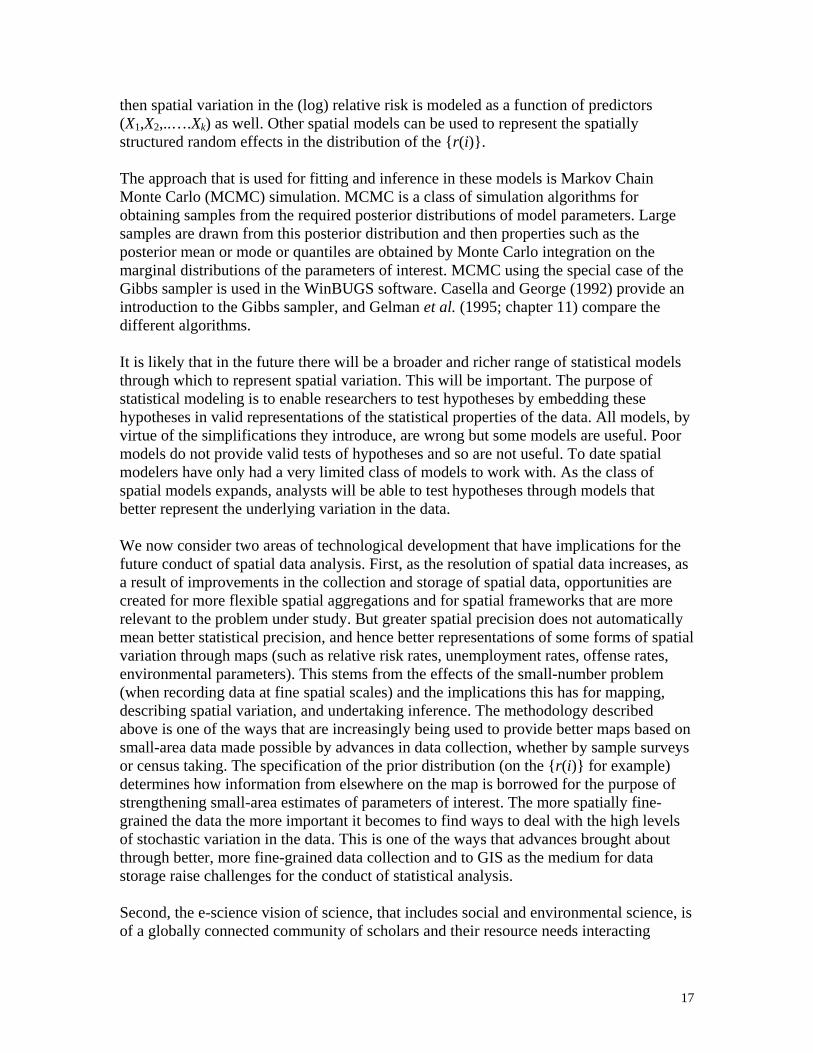
then spatial variation in the (log) relative risk is modeled as a function of predictors (X1,X2,..….Xk) as well. Other spatial models can be used to represent the spatially structured random effects in the distribution of the {r(i)}. The approach that is used for fitting and inference in these models is Markov Chain Monte Carlo (MCMC) simulation. MCMC is a class of simulation algorithms for obtaining samples from the required posterior distributions of model parameters. Large samples are drawn from this posterior distribution and then properties such as the posterior mean or mode or quantiles are obtained by Monte Carlo integration on the marginal distributions of the parameters of interest. MCMC using the special case of the Gibbs sampler is used in the WinBUGS software. Casella and George (1992) provide an introduction to the Gibbs sampler, and Gelman et al. (1995; chapter 11) compare the different algorithms. It is likely that in the future there will be a broader and richer range of statistical models through which to represent spatial variation. This will be important. The purpose of statistical modeling is to enable researchers to test hypotheses by embedding these hypotheses in valid representations of the statistical properties of the data. All models, by virtue of the simplifications they introduce, are wrong but some models are useful. Poor models do not provide valid tests of hypotheses and so are not useful. To date spatial modelers have only had a very limited class of models to work with. As the class of spatial models expands, analysts will be able to test hypotheses through models that better represent the underlying variation in the data. We now consider two areas of technological development that have implications for the future conduct of spatial data analysis. First, as the resolution of spatial data increases, as a result of improvements in the collection and storage of spatial data, opportunities are created for more flexible spatial aggregations and for spatial frameworks that are more relevant to the problem under study. But greater spatial precision does not automatically mean better statistical precision, and hence better representations of some forms of spatial variation through maps (such as relative risk rates, unemployment rates, offense rates, environmental parameters). This stems from the effects of the small-number problem (when recording data at fine spatial scales) and the implications this has for mapping, describing spatial variation, and undertaking inference. The methodology described above is one of the ways that are increasingly being used to provide better maps based on small-area data made possible by advances in data collection, whether by sample surveys or census taking. The specification of the prior distribution (on the {r(i)} for example) determines how information from elsewhere on the map is borrowed for the purpose of strengthening small-area estimates of parameters of interest. The more spatially fine-grained the data the more important it becomes to find ways to deal with the high levels of stochastic variation in the data. This is one of the ways that advances brought about through better, more fine-grained data collection and to GIS as the medium for data storage raise challenges for the conduct of statistical analysis. Second, the e-science vision of science, that includes social and environmental science, is of a globally connected community of scholars and their resource needs interacting

18

through virtual co-laboratories. One implication of this is the need for an information technology to support this where data, users and analysis services are spatially distributed (see also 3.1.2) . This will include shared access to large computing resources, large data archives, and data visualization techniques, and remote access to specialized facilities. The spatial analysis implication is not only for the development of appropriate numerical and visualization tools that can handle very large data sets, but in addition intelligent support systems to assist the analyst in all aspects of data handling and facilitating the extraction of useful information. Spatial analysis will move from only dealing with small regions or local scales of analysis (or large regions but at a coarser resolution) to larger scales of analysis. This in turn draws in problems of severe non-stationarity and complex patterns of association that need to be allowed for. In brief, a computationally intensive or demanding GIS requires analytical methods to support that scale of analysis. Modeling complex spatial structures calls for multi-level and multi-textured quantitative spatial data analysis. This calls for methods of spatial statistical and spatial mathematical modeling and complex forms of simulation that are enabled by improvements in computing power. 3.2.2 Applications and approaches to modeling The methods of spatial data analysis have been developed for, and implemented in, many different contexts. In early applications spatial models were used to assess competition effects, as measured by yield, between plants grown a fixed distance apart (e.g., Mead, 1967; Whittle, 1954). Cliff and Ord (1973, 1981) used autocorrelation statistics so they could test the fit of Hagerstand-type spatial diffusion models to real data. Haining (1987) used unilateral spatial autoregressions to estimate population and income multipliers for towns organized in a central place system. Anselin (1988), treating the field as a branch of econometrics (spatial econometrics), developed a statistical modeling strategy, with software to implement the methodology (Spacestat) that follows the strategy used in certain forms of time-series econometric modeling. There are numerous examples of the use of spatial regression modeling in a wide variety of fields (see for example Haining, 1990, 2003). Spatial modeling is undergoing its own shifts of emphasis and bringing with it new challenges for spatial data analysis as to how to assess correspondence between model output and real data. We illustrate this point with reference to two examples. Approaches to understanding regional growth in the 1960s and 70s focused on the role of the export sector. Modeling was based on pre-defined regions between which factors of production would move as well as flows of goods. Regional econometric and input-output modeling were the analytical structures that implemented a top-down approach in which inter- and intra-regional relationships were specified usually in terms of large numbers of parameters. Economists' new economic geography is concerned with regional growth and with understanding how the operation of the economy at regional scales affects national economic performance (Krugman, 1995; Porter, 1998) and trade (Krugman, 1991). A central feature of Krugman's modeling is the "tug of war between forces that tend to promote geographical concentration and those that tend to oppose it - between

19

'centripetal' and 'centrifugal' forces" (Krugman, 1996). The former includes external economies such as access to markets, and natural advantages. The latter includes external diseconomies such as congestion and pollution costs, land rents, and immobile factors. At the centre of new economic geography models is a view of the space economy as a complex, self-organizing, adaptive structure. It is complex in the sense of large numbers of individual producers and consumers. It is self organizing through invisible hand-of-the-market processes. It is adaptive in the sense of consumers and producers responding to changes in tastes, lifestyles, and technology, for example. The new economic geography is based on increasing returns from which spatial structure is an emergent property (Waldrop, 1992). Model outputs are characterized by bifurcations so that shifts from one spatial structure to another can result from smooth shifts in underlying parameters. Krugman's deterministic models appear to share common ground, conceptually, with multi-agent models used in urban modeling. In multi-agent models active autonomous agents interact and change location as well as their own attributes. Individuals are responding not only to local but also to global or system-wide information. Spatial structure in the distribution of individuals is an emergent property, and multi-agent models, unlike those of the regional approach to urban modeling developed in the 1970s and 1980s, are not based on pre-defined zones and typically use far fewer parameters (Benenson, 1998). These stochastic models have been used to simulate the residential behaviour of individuals in a city. They have evolved from cellular automata modeling approaches to urban structure, but describe a dynamic view of human interaction patterns and spatial behaviors (Benenson, 1998; Xie, 1996). In Benenson's model the probability of a household migrating is a function of the local economic tension or cognitive dissonance the household experiences at its current location. The probability of moving to any vacant house is a function of the new levels of economic tension or cognitive dissonance that would be experienced at the new location. A point of interest with both multi-agent and cellular automata models is how complex structures, and changes to those structures, can arise from quite simple spatial processes and sparse parameterizations (Batty, 1998; Benenson, 1998; Portugali et al., 1994; White and Engelen, 1994). The inclusion of spatial interaction can lead to fundamentally different results on the existence and stability of equilibria that echo phase transition behavior in some physical processes (Follmer, 1974; Haining, 1985). It is the possibility of producing spatial structure in new parsimonious ways together with the fact that the introduction of spatial relationships into familiar models can yield new and in some cases surprising insights, that underlies the current interest in space in certain areas of thematic social science. This interest, as Krugman (1996) points out, is underpinned by new areas of mathematics and modern computing that make it possible to analyze these systems. Local-scale interactions between fixed elementary units, whether these are defined in terms of individuals or small areas, can affect both local and system-wide properties. This effect is also demonstrated through certain models of intra-urban retailing where pricing

20

at any site responds to pricing strategies at competitive neighbors (Haining et al., 1996; Sheppard et al., 1992). Multi-agent modeling adds another, system-wide level to the set of interactions, allowing individuals to migrate around the space responding to global and local conditions in different segments of the space. All of these forms of modeling raise questions about how model expectations should be compared with observed data for purposes of model validation, so that validation is based on more than the degree of visual correspondence with real patterns. One aspect involves comparing the spatial structure generated by model simulations with observed spatial structures, and this calls directly for methods of spatial data analysis. In terms of the technology of data acquisition, in terms of the storage and display of data using GIS, and in terms of modeling paradigms there is an increasing focus on the micro-scale. In terms of the way science is conducted there is an increasing focus on inter-disciplinarity, collaboration, and communication across traditional boundaries. Spatial data analysis will over the coming years be responding to changes in this larger picture. 4. CONCLUDING COMMENTS We began this review with comments about the differences between the world views represented by GIS and spatial data analysis, and with a discussion of their different roots. The past 40 years show ample evidence of convergence, as the two fields have recognized their essential complementarity. As science moves into a new era of technology-based collaboration and cyberinfrastructure, exploiting tools that are becoming increasingly essential to a science concerned with understanding complex systems, it is clear that GIS and spatial data analysis need each other, and are in much the same relationship as exists between the statistical packages and statistics, or word processors and writing. It is more and more difficult to analyze the vast amounts of data available to regional scientists, and to test new theories and hypotheses without computational infrastructure; and the existence of such infrastructure opens possibilities for entirely new kinds of theories and models, and new kinds of data. The two perspectives have also done much to stimulate each other's thinking. GIS is richer for the demands of spatial data analysis, and spatial data analysis is richer for the focus that GIS has brought to issues of representation and ontology. The whole-map, nomothetic approach to science is giving way to a new, place-centered approach in which variations over the Earth's surface are as potentially interesting as uniformity. The view of GIS as an intelligent assistant is giving way to a new view of GIS as a medium of communication, in which spatial data analysis is one of several ways of enhancing the message. GIS is in many ways the result of adapting generic technologies to the particular needs of spatial data. In that sense its future is assured, since there is no lack of new technologies in the pipeline. New technologies have also stimulated new science, as researchers have begun to think about the implications of new data sources, or new technology-based activities. These in turn have stimulated new kinds of analytic methods, and new

21

hypotheses about the geographic world. The process of stimulus and convergence that began in the 1960s with GIS and spatial data analysis is far from complete, and the interaction between them is likely to remain interesting and productive for many years to come. REFERENCES Anderson, T.W., 1971. The Statistical Analysis of Time Series. New York, Wiley. Angel, S. and G.M. Hyman, 1976. Urban Fields: A Geometry of Movement for Regional Science. London: Pion. Anselin, L., 1988. Spatial Econometrics: Methods and Models. Dordrecht: Kluwer Academic. Anselin, L., 1995. Local indicators of spatial association - LISA. Geographical Analysis 27: 93-115. Bartlett, M.S., 1955. An Introduction to Stochastic Processes. Cambridge: Cambridge University Press. Batty, M., 1998. Urban evolution on the desktop: simulation with the use of extended cellular automata. Environment and Planning A 30: 1943-1967. Benenson, I., 1998. Multi-agent simulations of residential dynamics in the city. Computing, Environment and Urban Systems 22: 25-42. Berry, B.J.L. and D.F. Marble, 1968. Spatial Analysis. Englewood Cliffs, NJ: Prentice Hall. Besag, J.E., 1974. Spatial interaction and the statistical analysis of lattice systems. Journal of the Royal Statistical Society B36: 192-225. Besag. J.E., J. York, and A. Mollié, 1991. Bayesian image restoration with two applications in spatial statistics. Annals of the Institute of Statistical Mathematics 43: 1-21. Besag, J. and J. Newell, 1991. The detection of clusters in rare diseases. Journal of the Royal Statistical Society A154: 143-55. Burrough, P.A. and A.U. Frank, editors, 1996. Geographic Objects with Indeterminate Boundaries. New York: Taylor and Francis. Casella, G. and E.I. George, 1992. Explaining the Gibbs sampler. The American Statistician 46: 167-174.

22

Chorley, R.J., 1972. Spatial Analysis in Geomorphology. London: Methuen. Cliff A.D. and J.K. Ord, 1973. Spatial Autocorrelation. London: Pion. Cliff, A.D. and J.K. Ord, 1981. Spatial Processes. London: Pion. Craig W.J., T.M. Harris, and D. Weiner, editors, 2002. Community Participation and Geographic Information Systems. London: Taylor and Francis. Cressie, N., 1984. Towards resistant geostatistics. In G. Verly, M. David, A.G. Journel, and A. Marechal, editors, Geostatistics for Natural Resources Characterization, pp 21-44. Dordrecht: Reidel. Cressie, N., 1991. Statistics for Spatial Data. New York: Wiley. Diggle, P., 1983. Statistical Analysis of Spatial Point Patterns. London: Academic Press. Diggle, P.J. and A.D. Chetwynd, A.D., 1991. Second-order analysis of spatial clustering for inhomogeneous populations. Biometrics 47: 1155-1163. Duckham, M., M.F. Goodchild and M.F. Worboys, 2003. Fundamentals of Geographic Information Science. New York: Taylor and Francis. Economist, 2003. The revenge of geography. The Economist March 15. Follmer, H., 1974. Random economies with many interacting agents. Journal of Mathematical Economics 1: 51-62. Foresman, T.W., 1998. The History of GIS: Perspectives from the Pioneers. Upper Saddle River, NJ: Prentice Hall PTR. Frank, A.U., J. Raper, and J.P. Cheylan, editors, 2001. Life and Motion of Socio-Economic Units. New York: Taylor and Francis. Gatrell, A.C., T.C. Bailey, P.J. Diggle, and B.S. Rowlingson, 1996. Spatial point pattern analysis and its application in geographical epidemiology. Transactions, Institute of British Geographers 21: 256-74. Geary, R.C., 1954. The contiguity ratio and statistical mapping. The Incorporated Statistician 5: 115-145. Gelman, A., J.B. Carlin, H.S. Stern, and D.B. Rubin, 1995. Bayesian Data Analysis. London: Chapman and Hall. Goodchild, M.F., 1992. Geographical information science. International Journal of Geographical Information Systems 6(1): 31-45.

23

Goodchild, M.F., 1998. Uncertainty: the Achilles heel of GIS? Geo Info Systems (November): 50-52. Goodchild, M.F., 2002. Measurement-based GIS. In W. Shi, P.F. Fisher, and M.F. Goodchild, editors, Spatial Data Quality. New York: Taylor and Francis, pp. 5-17. Greig-Smith, P., 1952. The use of random and contiguous quadrats in the study of the structure of plant communities. Annals of Botany 16: 293-316. Grenander, U. and M. Rosenblatt, 1957. Statistical Analysis of Stationary Time Series. New York: Wiley. Haining, R.P., 1985. The spatial structure of competition and equilibrium price dispersion. Geographical Analysis 17: 231-242. Haining, R.P., 1987. Small area aggregate income models: theory and methods with an application to urban and rural income data for Pennsylvania. Regional Studies 21: 519-30. Haining, R.P., 1990. Spatial Data Analysis in the Social and Environmental Sciences. Cambridge: Cambridge University Press. Haining, R.P., 1994. Designing spatial data analysis modules for GIS. In A.S. Fotheringham and P. Rogerson, editors, Spatial Analysis and GIS, pp. 45-63. London: Taylor and Francis. Haining, R.P., 2003. Spatial Data Analysis: Theory and Practice. Cambridge: Cambridge University Press. Haining, R.P., P. Plummer, and E. Sheppard, 1996. Spatial price equilibrium in interdependent markets: price and sales configuration. Papers of the Regional Science Association 75: 41-64. Johnston, J., 1963. Econometric Methods. New York: McGraw Hill. Kendall, M.G., 1976. Time Series. London: Griffin. Krishna Iyer, P.V.A., 1949. The first and second moments of some probability distributions arising from points on a lattice and their applications. Biometrika 36: 135-141. Krugman, P., 1991. Geography and Trade. London: MIT Press. Krugman, P., 1995. Development, Geography and Economic Theory. London: MIT Press.

24

Krugman, P., 1996. Urban concentration: the role of increasing returns and transport costs. International Regional Science Review 19: 5-30 Kulldorff, M. and N. Nagarwalla, 1995. Spatial disease clusters: detection and inference. Statistics in Medicine 14: 799-810. Langran, G., 1992. Time in Geographic Information Systems. New York: Taylor and Francis. Liverman, D. et al., editors, 1998. People and Pixels: Linking Remote Sensing and Social Science. Washington, DC: National Academy Press. Longley, P.A., M.F. Goodchild, D.J. Maguire, and D.W. Rhind, 2001. Geographic Information Systems and Science. New York: Wiley. Maguire, D.J., M.F. Goodchild, and D.W. Rhind, editors, 1991. Geographical Information Systems: Principles and Applications. Harlow, UK: Longman Scientific and Technical. MacEachren, A.M. and M. Monmonier, 1992. Introduction (to special issue on Geographic Visualization). Cartography and Geographic Information Systems 19: 197-200. Malinvaud, E., 1970. Statistical Methods of Econometrics. Amsterdam: North Holland Publishing Company. Matern, B., 1986. Spatial Variation. 2nd Edition. Berlin: Springer Verlag. Matheron, G. 1963. Principles of geostatistics. Economic Geology 58: 1246-1266. McHarg, I.L., 1992. Design with Nature. New York: Wiley. Mead, R., 1967. A mathematical model for the estimation of inter-plant competition. Biometrics 23: 189-205. Mollié, A., 1996. Bayesian mapping of disease. In A. Lawson, A. Biggeri, D. Bohning, E. Lesaffre, J.F. Viel, and R. Bertollini, editors, Markov Chain Monte Carlo in Practice: Interdisciplinary Statistics, pp. 359-79. London: Chapman and Hall. Moran, P.A.P., 1948. The interpretation of statistical maps. Journal of the Royal Statistical Society B10: 243-51. Moran, P.A.P., 1950. Notes on continuous stochastic phenomena. Biometrika 37: 17-23.

25

Openshaw, S., 1983. The Modifiable Areal Unit Problem. Concepts and Techniques in Modern Geography 38. Norwich, UK: GeoBooks. Openshaw, S., M. Charlton, C. Wymer, and A. Craft, 1987. A Mark 1 Geographical Analysis Machine for the automated analysis of point data sets. International Journal of Geographical Information Systems 1: 335-58. Peuquet, D.J., 2002. Representations of Space and Time. New York: Guilford. Porter, M.E., 1998. The Competitive Advantage of Nations. London: MacMillan. Portugali, J., I. Benenson, and I. Omer, 1994. Sociospatial residential dynamics: stability and instability within a self-organizing city. Geographical Analysis 26: 321-340. Ripley, B.D., 1977. Modelling spatial patterns. Journal of the Royal Statistical Society B39: 172-192. Ripley, B.D., 1981. Spatial Statistics. New York: Wiley. Sheppard, E., R. Haining, and P. Plummer, 1992. Spatial pricing in interdependent markets. Journal of Regional Science 32: 55-75. Stoyan, D., W.S. Kendall, and J. Mecke, 1989. Stochastic Geometry and Its Applications. New York: Wiley. Tomlinson, R.F., H.W. Calkins, and D.F. Marble, 1976. Computer Handling of Geographical Data: An Examination of Selected Geographic Information Systems. Paris: UNESCO Press. Ungerer, M.J. and M.F. Goodchild, 2002. Integrating spatial data analysis and GIS: a new implementation using the Component Object Model (COM). International Journal of Geographical Information Science 16(1): 41-54. University Consortium for Geographic Information Science, 1996. Research priorities for geographic information science. Cartography and Geographic Information Science 23(3). Waldrop, M.W., 1992. Complexity. New York: Simon and Schuster. White, R. and G. Engelen, 1994. Cellular dynamics and GIS: modeling spatial complexity. Geographical Systems 1: 237-253. Whittle, P., 1954. On stationary processes in the plane. Biometrika 41: 434-49.

26

Wold, H., 1954. A Study in the Analysis of Stationary Time Series. Uppsala: Almqvist and Wiksells. Xie, Y., 1996. A generalized model for cellular urban dynamics. Geographical Analysis 28: 350-373. Zhang, J.X. and M.F. Goodchild, 2002. Uncertainty in Geographical Information. New York: Taylor and Francis.