Embed Size (px)
Citation preview

Getting Started with Survival Analysis
Course Notes

Getting Started with Survival Analysis Course Notes was developed by Marc Huber. Editing and production support was provided by the Curriculum Development and Support Department.
SAS and all other SAS Institute Inc. product or service names are registered trademarks or trademarks of SAS Institute Inc. in the USA and other countries. ® indicates USA registration. Other brand and product names are trademarks of their respective companies.
Getting Started with Survival Analysis Course Notes
Copyright © 2018 SAS Institute Inc. Cary, NC, USA. All rights reserved. Printed in the United States of America. No part of this publication may be reproduced, stored in a retrieval system, or transmitted, in any form or by any means, electronic, mechanical, photocopying, or otherwise, without the prior written permission of the publisher, SAS Institute Inc.
Course code SGF18SRV, prepared date 09Mar2018. SGF18SRV_001

For Your Information iii
Table of Contents
To learn more… ................................................................................................... iv
Chapter 1 Introduction to Survival Analysis ............................................................. 1-1
1.1 Survival Analysis Concepts ...................................................................................... 1-3
1.2 Exploratory Data Analysis Using Survival Curves .................................................. 1-12
Demonstration: Comparing Survival Functions ................................................. 1-25
1.3 Chapter Summary .................................................................................................. 1-37
Chapter 2 Proportional Hazards Model ..................................................................... 2-1
2.1 Introduction to the Cox Proportional Hazards Model ................................................ 2-3
Demonstration: Cox Proportional Hazards Model ............................................. 2-16
Demonstration: Adjusted Survival Curves ........................................................ 2-22
2.2 Chapter Summary .................................................................................................. 2-29
Appendix A References ................................................................................................ A-1
A.1 References.............................................................................................................. A-3

iv For Your Information
To learn more…
For information about other courses in the curriculum, contact the SAS Education Division at 1-800-333-7660, or send e-mail to [email protected]. You can also find this information on the web at http://support.sas.com/training/ as well as in the Training Course Catalog.
For a list of SAS books (including e-books) that relate to the topics covered in this course notes, visit https://www.sas.com/sas/books.html or call 1-800-727-0025. US customers receive free shipping to US addresses.

Chapter 1 Introduction to Survival Analysis
1.1 Survival Analysis Concepts ................................................................................................. 1-3
1.2 Exploratory Data Analysis Using Survival Curves .......................................................... 1-12
Demonstration: Comparing Survival Functions ................................................................... 1-25
1.3 Chapter Summary .............................................................................................................. 1-37

1-2 Chapter 1 Introduction to Survival Analysis
Copyright © 2018, SAS Institute Inc., Cary, North Carolina, USA. ALL RIGHTS RESERVED.

1.1 Survival Analysis Concepts 1-3
Copyright © 2018, SAS Institute Inc., Cary, North Carolina, USA. ALL RIGHTS RESERVED.
1.1 Survival Analysis Concepts
Copyright © SAS Inst itute Inc. A l l r ights reserved.
3
What Is Survival Analysis?
• Survival analysis is a class of statistical methods for which the outcome variable of interest is time until an event occurs.
• Time is measured from the beginning of follow-up until the event occurs or a reason occurs for the observation of time to end.
Survival analysis is a collection of specialized methods used to analyze data in which time until an event occurs is the response variable of interest. The response variable, often called in survival analysis a failure time, survival time, or event time, is usually continuous and can be measured in days, weeks, months, years, and so on. Events can be deaths, onset of disease, marriages, arrests, and so on. What is unique about survival analysis is that even if the subject did not experience an event, the subject’s survival time or length of time in the study is taken into account.

1-4 Chapter 1 Introduction to Survival Analysis
Copyright © 2018, SAS Institute Inc., Cary, North Carolina, USA. ALL RIGHTS RESERVED.
Copyright © SAS Inst itute Inc. A l l r ights reserved.
4
Examples of Survival Analysis
• Follow-up of patients undergoing surgery to measure how long they survived after the surgery
• Follow-up of leukemia patients in remission to measure how long they remain in remission
• Follow-up of newly released parolees to measure how long it is from date of release until date of re-arrest
Survival analysis is used heavily in clinical and epidemiological follow-up studies. Other fields that use survival analysis methods include sociology, engineering, and economics. Survival analysis is also known as time to event analysis, reliability analysis, durability analysis, event history analysis, and lifetime analysis, among others. Regardless of the field, the common objective of a survival analysis study is not only whether an event occurred, but also when it occurred. For example, subjects that die 5 years after surgery are different from subjects that die 1 month after surgery. An analysis that simply counted deaths would ignore valuable information about survival time.
Survival analysis can also be used to analyze outcomes other than time. For example, an engineer might want to analyze the amount of mileage until a tire fails or the number of cycles until an engine requires repair. What is common across these studies is that you are analyzing an outcome until an event occurs, and that outcome does not necessarily have to be time.

1.1 Survival Analysis Concepts 1-5
Copyright © 2018, SAS Institute Inc., Cary, North Carolina, USA. ALL RIGHTS RESERVED.
Copyright © SAS Inst itute Inc. A l l r ights reserved.
5
What Is Survival Analysis?
Time
Subjects
A
B
C
D
E
F
G
1 2 3 4 5 6
End of Study
Withdrew
Lost to Follow-up
Censored Event
Survival can be envisioned as timelines for individual subjects that are considered at risk of experiencing a particular type of event. The timeline is not always a complete record, and some subjects might have an event outside of the time frame during which they are observed.
Copyright © SAS Inst itute Inc. A l l r ights reserved.
6
Censoring
Censoring occurs when the event time is not observed.
Types:
• Right Censoring
• Type I
• Type II
• Interval
• Left Censoring
• Interval Censoring

1-6 Chapter 1 Introduction to Survival Analysis
Copyright © 2018, SAS Institute Inc., Cary, North Carolina, USA. ALL RIGHTS RESERVED.
Survival analysis allows the response variable to be incompletely determined for some subjects. Exact failure time remains unknown. When this occurs, it is called censoring. These subjects should not be ignored. The time that they are observed contributes information to the study. Ignoring them completely adds bias to the estimates of population survival time. Neither should they be assumed to have had the event at the closest observed time point because event times (assuming an event eventually occurs) reported that way would be inaccurately measured.
Censoring is categorized into three main types, right, left and interval, depending on where the lack of information exists on the timeline relative to the observed follow-up times.
Copyright © SAS Inst itute Inc. A l l r ights reserved.
7
Right Censoring
An observation is right-censored if the observation is terminated before the event occurs.
Time
Subjects
B
C
E
1 2 3 4 5 6
End of Study
Withdrew
Lost to Follow-up
There are several types of censoring. Subjects are right-censored if the only information that you know about their survival time is that it is greater than some value t. It is named right-censored because the subject’s survival time becomes incomplete at the right side of the follow-up period. In other words, you only know that the event did not happen at the indicated time, so it must happen at some time in the future.

1.1 Survival Analysis Concepts 1-7
Copyright © 2018, SAS Institute Inc., Cary, North Carolina, USA. ALL RIGHTS RESERVED.
Copyright © SAS Inst itute Inc. A l l r ights reserved.
8
Left Censoring
An observation is left-censored when the observation experiences the event before the start of the follow-up period.
Start of Study
End of Study
G
H
Time before Study
Event
Event
Subjects are left-censored if the only information you know that an event occurred before follow-up began, but you do not know exactly when it occurred. The subjects’ survival time becomes incomplete at the left side of the follow-up period. This can happen in studies when you begin to observe a cohort at a time when some of the subjects might have already experienced the event. This is different from left truncation, where an unknown subset of subjects failed before a certain time and the subjects did not participate in the study.

1-8 Chapter 1 Introduction to Survival Analysis
Copyright © 2018, SAS Institute Inc., Cary, North Carolina, USA. ALL RIGHTS RESERVED.
Copyright © SAS Inst itute Inc. A l l r ights reserved.
9
Interval Censoring
An observation is interval-censored if the only information that you know about the survival time is that it is between the values t and t+k.
A
B
Event
Event
Time
Observed time t
Observed time t+k
Subjects are interval-censored if the only information that you know about their survival time is that it is between two time points. This occurs in studies when observations are recorded at infrequent intervals. For example, when the presence of a medical condition is assessed during periodic exams, the time until the condition developed is only known to be between the current and previous exam. The exact timing of the event is unavailable.
Note: Gaps in observation are routine in nearly all longitudinal studies involving human subjects. The imprecision of event time measurement can be ignored if the interval is not too great. If that is the case, several event times can appear to be tied. Ties will be discussed in a later chapter.
Note: Neither left-censored nor interval-censored data will be analyzed in this course. The Cox proportional hazards regression model will not handle left-censored or interval-censored data. SAS can analyze left- or interval-censored data in either the LIFEREG or ICPHREG procedures.

1.1 Survival Analysis Concepts 1-9
Copyright © 2018, SAS Institute Inc., Cary, North Carolina, USA. ALL RIGHTS RESERVED.
Copyright © SAS Inst itute Inc. A l l r ights reserved.
10
Data Structure
Subject Survival Time Status
A 4.0 1 (event)
B 6.0 0 (censored)
C 3.0 0
D 5.0 1
E 3.0 0
F 3.0 1
G 2.0 1
Note: Survival Time is relative time – relative to some time origin.
The data layout for survival analysis requires that one variable represents survival time information. Each of the subjects has an observed survival time regardless of whether the subject experienced the event or was censored. To distinguish the subjects who were censored from those who experienced the event, a variable that indicates censorship status is required. If there is only one type of event, then this variable usually equals 1 for subjects who experienced the event and 0 for subjects who were censored. Survival analysis data can also include time-independent and time-dependent explanatory variables.
Note: The data layout shown above corresponds to the timeline diagram in a previous slide.

1-10 Chapter 1 Introduction to Survival Analysis
Copyright © 2018, SAS Institute Inc., Cary, North Carolina, USA. ALL RIGHTS RESERVED.
Copyright © SAS Inst itute Inc. A l l r ights reserved.
11
Problems with Conventional Methods
Logistic regression
• ignores information about the timing of events
• cannot handle time-dependent covariates.
Linear regression
• cannot handle censored observations
• cannot handle time-dependent covariates
• is not appropriate because time to event can have unusual distribution.
Survival analysis methods in SAS software can handle two common features of survival analysis data: censoring and time-dependent explanatory variables. Even if no subjects were censored and no variables were time-dependent, conventional methods such as linear regression would still not be appropriate. First, because the response variable must take on positive values, the distribution is probably skewed and is likely not to be normal. Furthermore, the results of linear regression would give you the expected survival time, while survival analysis methods would give you the probability of surviving past a certain time, which is often more relevant (Harrell 1997).
Copyright © SAS Inst itute Inc. A l l r ights reserved.
12
Survival Analysis
The goals of survival analysis might be the following:
• to estimate and interpret survival and hazard functions from survival data
• to compare survival and hazard functions among different groups
• to assess the relationship of time-independent and time-dependent explanatory variables to survival time
• to predict the remaining time until the event

1.1 Survival Analysis Concepts 1-11
Copyright © 2018, SAS Institute Inc., Cary, North Carolina, USA. ALL RIGHTS RESERVED.
The first step in the analysis of survival data is to examine the distribution of survival time. This can be accomplished by plotting the survival function and the hazard function. Another step is to build a model that describes the relationship between the distribution of survival time and the explanatory variables. Assessing the fit of the model and computing adjusted survival functions are also important steps in the analysis of survival data.
Building predictive models that predict the remaining time until the event is another application of survival analysis. The course notes that addresses predictive modeling using survival data is called Survival Data Mining: Predictive Hazard Modeling for Customer History Data.

1-12 Chapter 1 Introduction to Survival Analysis
Copyright © 2018, SAS Institute Inc., Cary, North Carolina, USA. ALL RIGHTS RESERVED.
1.2 Exploratory Data Analysis Using
Survival Curves
Copyright © SAS Inst itute Inc. A l l r ights reserved.
15
Survival Function
Usually, the first step in the analysis of survival data is to estimate and plot the survival function. The survival function gives the probability that a subject survives longer than some specified time t. This can be defined by the formula ( ) Pr( )S t T t where T is a random variable for a person’s survival
time and t is any specific value of interest. At t=0, S(0)=1 (at the start of the study, because no one
has experienced the event yet, the probability of surviving past time 0 is 1) while at t=, S()=0 (eventually nobody survives, so the survival function theoretically must fall to 0). As t increases, S(t) never increases and usually decreases. The factors that influence the shape of the survival function are when the subjects experience the event, when the subjects were censored, and the pattern of enrollment in the follow-up study (Hosmer and Lemeshow 1999). In practice, the survival function resembles a decreasing step function rather than a smooth curve. Furthermore, because not everyone might experience the event by the end of the study (they are Type I censored), the survival function might not reach 0.
If there is no censoring or if the censored times are all greater than the event times, then it is relatively easy to estimate the survival function. Calculate the proportion of cases that have survived past time point t. However, if some censored times are less than the event times, then the censored observations must be taken into account. One method that considers censored observations is the Kaplan-Meier method.
The Kaplan-Meier method incorporates information from all the observations available, both censored and non-censored, to compute survival probabilities at a given time (Kaplan and Meier, 1958). Rather than ignore the information about a censored subject, this method uses the information about the censored subject up to the time the subject becomes censored.
To illustrate the Kaplan-Meier method, revisit the example data set from the previous section.

1.2 Exploratory Data Analysis Using Survival Curves 1-13
Copyright © 2018, SAS Institute Inc., Cary, North Carolina, USA. ALL RIGHTS RESERVED.
Copyright © SAS Inst itute Inc. A l l r ights reserved.
16
Kaplan-Meier Method
16
Time
Number
Events
Number
Censored
0 0 0
1 0 0
2 1 0
3 1 2
4 1 0
5 1 0
6 0 1
Number
At Risk
Cumulative
Survival
7 1.00
7 1.00
7 6/7=.86
6 .86*5/6=.71
3 .71*2/3=.48
2 .48*1/2=.24
1 --------------
The above slide uses the example data set, partitioned by each distinct event time, to illustrate the Kaplan-Meier method. At time 0, there were no events and no censored observations. The Number At Risk column enumerates the observations that have not experienced an event or have not been censored at the beginning of the time point. Thus, at time 0, there are 7 subjects at risk of having the event. The Cumulative Survival column shows the Kaplan-Meier estimator. At time 0 the estimator is 1, because the probability of surviving past time 0 is 1.
At time 2, there was 1 event. Thus, the probability of surviving past time 2 is 6/7 or .86 ((number at risk – number of events) / number at risk). At time 3, there was 1 event and 2 censored observations. The number at risk was 6, because 6 subjects survived past time 2. The Kaplan-Meier estimator is computed by multiplying the probability of surviving past the previous time point (.86) by the conditional probability of surviving past time 3, given survival to at least time 3 (5/6).
At time 4, there was 1 event. The number at risk was 3 because only 3 subjects survived past time 3. The Kaplan-Meier estimator is computed by multiplying the probability of surviving past the previous time point (.71) by the conditional probability of surviving past time 4, given survival to at least time 4 (2/3). The same result could be obtained by multiplying the sequence of conditional survival probabilities (1*6/7*5/6*2/3=.48).
Therefore, the Kaplan-Meier estimator allows each subject to contribute information to the calculations as long as the subjects are in the study. Subjects that experience the event contribute to the number at risk until their time of the event. Subjects that are censored contribute to the number at risk until they are censored. Notice that subjects who are censored are assumed to be at risk for the whole time point.
At time 6, there was 1 censored observation and 1 observation at risk. The estimator is undefined because not all subjects experienced the event by time 6 and no follow-up extends beyond time 6.

1-14 Chapter 1 Introduction to Survival Analysis
Copyright © 2018, SAS Institute Inc., Cary, North Carolina, USA. ALL RIGHTS RESERVED.
Copyright © SAS Inst itute Inc. A l l r ights reserved.
17
Kaplan-Meier Curve
This slide illustrates the Kaplan-Meier curve for the example data set. Notice that the curve is a decreasing step function that drops at the values of the observed event times and is constant between the event times. At time 2, the Kaplan-Meier estimator is 0.86, which corresponds to the previous slide.

1.2 Exploratory Data Analysis Using Survival Curves 1-15
Copyright © 2018, SAS Institute Inc., Cary, North Carolina, USA. ALL RIGHTS RESERVED.
Copyright © SAS Inst itute Inc. A l l r ights reserved.
18
Hazard Function
• The hazard function is the instantaneous risk or potential that an event will occur at time t, given that the individual has survived up to time t.
• It takes the form number of events per interval of time.
• It is a rate, not a probability, that ranges from zero to infinity.
Another way to describe the distribution of survival times is to examine the hazard function. This function is essentially an instantaneous event rate that enables you to examine the forces of risk over time. In other words, the hazard is expressed as the expected number of events in a one-unit interval of time. For example, if the event is ear infections and the hazard rate in year 4 is 2.0, then the subjects who survived to year 4 are expected to have ear infections 2 times during year 4. In other words, the rate of ear infections at year 4 is 2 per year.
Unlike the survival function, the hazard function does not have to start at 1 and end at 0. This function can begin anywhere and move up and down in any direction over time. Other properties of the hazard function are that it is always nonnegative and has no upper bound. It also has a clearly defined relationship with the survival function. In fact, if you know the form of the survival function, then you can derive the corresponding hazard function, and vice versa.
The formula for the survival function expressed in terms of the hazard function is
0
( )
( )
t
h u du
S t e
The formula shows that the survival function is equal to the exponential of the negative integral of the hazard function between the integration limits of 0 and t (Kleinbaum 1996).
The formula for the hazard function expressed in terms of the survival function is
( )
( )( )
dS t
dth tS t

1-16 Chapter 1 Introduction to Survival Analysis
Copyright © 2018, SAS Institute Inc., Cary, North Carolina, USA. ALL RIGHTS RESERVED.
The formula shows that the hazard function is equal to minus the derivative of the survival function with respect to t divided by the survival function (Kleinbaum 1996).
Copyright © SAS Inst itute Inc. A l l r ights reserved.
19
Hazard Rate Example
• Indicates how great the risk is for events at a given moment.
• Shows instantaneous risk or potential of how many events you will have in the given time period.
...
1.2 events per year
To understand the concept of the hazard rate, consider the concept of velocity. If you drive at 50 miles per hour, then in the next hour if you maintain the same speed, then you will travel 50 miles. The speedometer shows you the potential or risk of how many miles you will travel in the next hour.
The hazard rate is similar to velocity in that it gives the instantaneous rate at a given time for getting an event, given survival up to that given point in time. The rate is a conditional rate because it only applies to the subset of the sample that has survived to a particular point (the number at risk for the event).

1.2 Exploratory Data Analysis Using Survival Curves 1-17
Copyright © 2018, SAS Institute Inc., Cary, North Carolina, USA. ALL RIGHTS RESERVED.
Copyright © SAS Inst itute Inc. A l l r ights reserved.
20
Hazard Function
0
( | )( ) lim
t
P t T t t T th t
t
Instantaneous risk or potential
Interval of time
Conditional Probability
The numerator of the hazard function is a conditional probability that gives the probability that the
event will occur in the time interval between t and t + t given survival to time t. To adjust for the time
interval, the denominator for the hazard function is t, which makes the hazard function a rate rather than a probability. Finally, to make the rate an instantaneous rate at exactly time t, the formula takes the limit of the expression as the time interval approaches 0. Thus, the formula is shrinking the time
interval by allowing t to become smaller and smaller until it reaches a limiting value.

1-18 Chapter 1 Introduction to Survival Analysis
Copyright © 2018, SAS Institute Inc., Cary, North Carolina, USA. ALL RIGHTS RESERVED.
Copyright © SAS Inst itute Inc. A l l r ights reserved.
21
Comparing Survival Functions
A useful graph in exploratory data analysis is a graph that compares survival functions across groups. In the plot at the upper left, the female survival function lies above the male survival function, which means females had a more favorable survival experience. If the event was death, then at any point in time the proportion of females estimated to be alive is larger than the proportion of males estimated to be alive.
A graph comparing survival functions can also give insight to how time is related to the survival experience across groups. It can indicate interactions with time. In the plot at the upper right, subjects in Clinic 1 have a more favorable survival experience than subjects in Clinic 2. However, the differences between the groups are relatively small in the early time points and get progressively larger in the later time points. Early in the study, both clinics lost a similar proportion of patients. However, as the study progressed, the patients in Clinic 1 had much longer survival times compared to the patients in Clinic 2.
An interaction between time and group can mean that the group survival distributions cross. In the plot at the lower left, subjects taking Drug B have a more favorable survival experience in the early time points but a worse survival experience in the later time points when compared to subjects taking Drug A.
If there are more than 2 groups, then a graph comparing survival functions can illustrate which groups have relatively similar survival experiences and which groups have relatively different survival experiences. In the plot at the lower right, the subjects with the high dose have more favorable survival experiences compared to subjects with the medium dose and the low dose. A useful test would be a multiple comparisons test to see which groups have significantly different survival distributions.

1.2 Exploratory Data Analysis Using Survival Curves 1-19
Copyright © 2018, SAS Institute Inc., Cary, North Carolina, USA. ALL RIGHTS RESERVED.
Copyright © SAS Inst itute Inc. A l l r ights reserved.
22
Nonparametric Homogeneity Tests
where wj is the weight at time j, d1j is the number of events in group 1 at time j, and e1j is the expected number of events in group 1 at time j.
• can be biased if the pattern of censoring is different between the groups.
• have problems in the presence of interactions.
2
1 1
1
1 1
1
( )
var ( )
r
j j j
j
r
j j j
j
w d e
w d e
After the survival functions are plotted, it is of interest to determine whether there are statistically significant differences among the survival functions. In other words, is there a difference in the event time distributions between the groups? The most frequently used and reported k-sample test for the comparison of survival functions is the log-rank test. This test is a nonparametric test that requires no assumptions regarding the distribution of event times (which is useful because the distribution of event times will be right-skewed).
The log-rank test is an application of the Cochran-Mantel-Haenszel test where the contingency table is grouped by event status, and the time points define the strata. The null hypothesis is that the distribution of event times is equal among the groups while the alternative hypothesis is that the distribution of event times differs between groups.
For two groups, if the ratio of the hazards is constant over time and the censoring distributions are the same, then the log-rank test will have maximal power compared to other differences in survival function tests (Cantor 1997). For this reason it is important to check the patterning of censoring for each group (Hosmer and Lemeshow 1999). If the assumption that the ratio of hazards is constant over time is valid, then the plot of the log of the negative log of the survival function versus the log of time should show parallel curves.
The formula for the log-rank test for 2 groups shows that the statistic is computed by summing the observed minus expected counts over all the time points for one of the groups, squaring that quantity, and then dividing by the estimated variance of the summed observed minus expected counts. Under the null hypothesis, the log-rank statistic is approximately chi-square with one degree of freedom. The number of time points goes from 1 to r.
The Wilcoxon test is similar to the log-rank test except that it weights the observed number of events minus the expected number of events by the number at risk across the event times. The weights are equal to the number at risk.

1-20 Chapter 1 Introduction to Survival Analysis
Copyright © 2018, SAS Institute Inc., Cary, North Carolina, USA. ALL RIGHTS RESERVED.
Because the number at risk depends on both the number censored as well as the survival experience, the pattern of censoring can bias the Wilcoxon test. For example, if the pattern of censoring is markedly different between the groups, then this test might reject the null hypothesis based on the pattern of censoring rather than the differences in survival experience. For this reason, it is critical to examine the pattern of censoring among the groups (Hosmer and Lemeshow 1999).
The pattern of censoring might be different between the groups because of problems in the study design and problems in data collection. The best protection from these problems is a carefully designed study that increases the likelihood that the pattern of censoring is independent of the group (Hosmer and Lemeshow 1999).
The log-rank test puts the same weight on all parts of the survival function. However, the Wilcoxon test uses weights equal to the number at risk. Because the number at risk decreases as the study progresses, the Wilcoxon test puts relatively more weight on differences between the survival functions in the early points in time while the log-rank test is more sensitive to differences between groups in later points in time. Therefore, if you want to emphasize earlier failure times in your study, then the Wilcoxon test is more appropriate than the log-rank test. However, both tests should be reported if the tests give different results. This provides a clearer picture as to where the survival functions are different and if the pattern of censoring is affecting the Wilcoxon test (Kleinbaum 1996).

1.2 Exploratory Data Analysis Using Survival Curves 1-21
Copyright © 2018, SAS Institute Inc., Cary, North Carolina, USA. ALL RIGHTS RESERVED.
Copyright © SAS Inst itute Inc. A l l r ights reserved.
23
Nonparametric Tests in PROC LIFETEST
Several statistical nonparametric tests for comparing survival functions have been incorporated in PROC LIFETEST. The differences among the nonparametric tests are in the choice of weight functions weights applied to the deviations between observed and expected numbers of events in the numerator and denominator of the Log-rank test.
Tarone-Ware test uses a weight equal to the square root of the number at risk. This gives more weight to differences between the observed and expected number of events at time points where there is the most data.
Peto-Peto and Modified Peto-Peto tests use weights that depend of the observed survival experience of the combined sample. The principal advantage of these tests is that they do not depend on the censoring experience of the groups (Hosmer and Lemeshow 1999).
Harrington-Fleming family of tests incorporates features of both the log-rank and Peto-Peto tests. It uses a survival function where the previous event time is used as a weight to ensure that these weights are known just prior to the time at which the comparison is to be made. The values of p and q must be greater than or equal to zero. When p and q are 0, the Harrington-Fleming test is the log-rank test. If p is 1 and q is 0, then the test becomes a version of the Wilcoxon test. If q is 0 and p is greater than 0, then the weights give the most weight to early departures of the survival functions. If p is 0 and q is greater than 0, then the test gives more weight to departures that occur late in time. Therefore, with the appropriate choice of the values of p and q, you can construct a test that has the most power to detect differences over any desired region of the time interval (Klein and Moeschberger 1997).
It should be noted that all of these nonparametric tests are based on large-sample approximations to the distribution of the chi-square statistics. They also assume that the censoring distributions are independent of the event distributions. Care should be used in interpreting these results when the sample sizes are small or when there are few events (Klein and Moeschberger 1997).

1-22 Chapter 1 Introduction to Survival Analysis
Copyright © 2018, SAS Institute Inc., Cary, North Carolina, USA. ALL RIGHTS RESERVED.
Copyright © SAS Inst itute Inc. A l l r ights reserved.
24
Likelihood-Ratio Test
• The likelihood-ratio test is a parametric test that assumes that the distribution of event times follows an exponential distribution.
• It can be verified if the plot of the negative log of the survival function by time follows a linear trend with an origin of 0.
Another test that compares the survival functions is the likelihood-ratio test. Unlike the nonparametric tests, this test is a parametric test that assumes the event times follow an exponential distribution. This means that the hazard function is constant in each group. When this assumption is true, the likelihood-ratio test is more powerful than the other two tests (Allison 1995).
If the distribution of event times is exponential, then a plot of the negative log of the survival function versus time should yield a straight line with an origin of 0. This plot can help verify whether the exponential assumption is valid and whether the likelihood-ratio test should be used when comparing survival functions (Allison 1995).

1.2 Exploratory Data Analysis Using Survival Curves 1-23
Copyright © 2018, SAS Institute Inc., Cary, North Carolina, USA. ALL RIGHTS RESERVED.
Copyright © SAS Inst itute Inc. A l l r ights reserved.
25
LIFETEST Procedure
General form of the LIFETEST procedure:
PROC LIFETEST DATA=SAS-data-set <options>;TIME variable <*censor(list)>;STRATA variable <(list)> <...variable <(list)>>
</options>;TEST variables;
RUN;
The LIFETEST procedure computes and plots survival functions and tests for differences between survival functions. The PROC LIFETEST and TIME statements are required, and there is no required order for the statements following the PROC LIFETEST statement. The TIME statement is used to specify the variables that define the survival time and the censoring indicator. The STRATA statement specifies a variable or set of variables defining the strata for the analysis. When the STRATA statement is used, the tests that compare survival functions are computed. The TEST statement specifies a list of numeric predictor variables to be tested for their association with the response survival time. Each variable is tested individually, and a joint test statistic is also computed.
Selected PROC LIFETEST statement options:
PLOTS= controls the plots produced using ODS Graphics.
Selected PROC LIFETEST statements:
TIME indicates the survival time variable and the censoring variable. A parenthetical list of values that correspond to right censoring follows the censoring variable. The censoring values should be numeric, nonmissing values.
STRATA indicates which variables define the strata. If the variable is a character variable or if the variable is numeric and no list appears, then the strata are defined by the unique values of the strata variable. If the variable is numeric and followed by a list, then the levels correspond to the intervals defined by the list.
TEST indicates the numeric predictor variables to be tested for the association with survival time.
Selected STRATA statement option:
TEST= controls the tests produced. Each test corresponds to a different weight function.

1-24 Chapter 1 Introduction to Survival Analysis
Copyright © 2018, SAS Institute Inc., Cary, North Carolina, USA. ALL RIGHTS RESERVED.
Copyright © SAS Inst itute Inc. A l l r ights reserved.
26
Methadone Treatment Data
Clinic (1 or 2)
Days spent in Clinic
Methadone Dosage (mg / day)
Prison Record(0=No, 1=Yes)
Example: A study was conducted to investigate the differences in survival experience between two methadone treatment programs (Clinic 1 versus 2). The outcome variable is the number of days patients spend in a methadone treatment program. The event is dropping out of the program and the observation is censored if the patient transferred to another program or survived to the end of the study. The predictor variables that are believed to affect survival time are prison record and methadone dose. The data are stored in a SAS data set called sasuser.methadone.
These are the variables in the data set:
Clinic Clinic (1 or 2)
Status survival status (0=censored, 1=departed from clinic)
Time survival time in days spent in clinic
Prison prison record (0=no, 1=yes)
Dose methadone dosage (mg/day)
Note: The data were obtained with permission from the Australasian Data and Story Library (OZDasl - http://www.statsci.org/data) website. The study in which the data was collected is described in Caplehorn et al. (1991).

1.2 Exploratory Data Analysis Using Survival Curves 1-25
Copyright © 2018, SAS Institute Inc., Cary, North Carolina, USA. ALL RIGHTS RESERVED.
Comparing Survival Functions
Example: Compute the survival function and the cumulative hazard rate for each clinic in the sasuser.methadone data set. Request the log-rank test of equality over strata and specify the arcsine-square root transformation to be applied to the survival function to obtain confidence intervals for the quartiles of the survival times. Use ODS Statistical Graphics to plot the survival functions displaying the number of subjects at risk at time 0 to 1000 by 100 and the p-value of the log-rank test, the negative log of survival time versus time, and the log negative log of survival time versus the log of time.
/*surv01d01.sas*/ /*Part A*/
ods graphics on;
proc lifetest data=sasuser.methadone
nelson
conftype=asinsqrt
plots=(survival(atrisk=0 to 1000 by 100 test)
loglogs
logsurv);
time time*status(0);
strata clinic / test=all;
test dose prison;
title "Survival Functions for Methadone Data";
run;
Selected PROC LIFETEST statement option:
NELSON produces the Nelson-Aalen estimates of the cumulative hazards and the corresponding standard errors. This option is ignored unless METHOD=PL.
Selected plot requests:
SURVIVAL plots the estimated survivor functions. Censored times are plotted as a plus sign on the product-limit curves unless the NOCENSOR option is specified.
LOGLOGS plots the log of negative log of estimated survivor functions versus the log of time.
LOGSURV plots the negative log of estimated survivor functions versus time.
Selected survival plot options:
ATRISK<number list> displays the numbers of subjects at risk at the given times. The number-list identifies the times at which the numbers at risk are displayed. If the number-
list is not specified, PROC LIFETEST uses an algorithm to specify the time points.
TEST displays the p-value of a homogeneity test specified in the STRATA statement. If more than one test is produced, the test is chosen in the following order: LOGRANK, WILCOXON, TARONE, PETO, MODPETO, FLEMING, and LR.
Selected STRATA statement option:
TEST= controls the tests produced. Each test corresponds to a different weight function. The test requests include the following:

1-26 Chapter 1 Introduction to Survival Analysis
Copyright © 2018, SAS Institute Inc., Cary, North Carolina, USA. ALL RIGHTS RESERVED.
ALL specifies all the nonparametric tests with p1=1 and p2=0 for the Fleming and Harrington test—FLEMING(1,0).
FLEMING(p,q) specifies a family of tests where p1and p2are nonnegative numbers. FLEMING(p,q) reduces to the Fleming-Harrington Gp family (when q=0, which you can specify as FLEMING(p) with one argument. When p=0, the test becomes the log-rank test. When p=1, the test should be very close to the Peto-Peto test.
LOGRANK specifies the log-rank test.
NONE suppresses all comparison tests. Specifying TEST=NONE is equivalent to specify NOTEST.
LR specifies the likelihood ratio test based on the exponential model.
MODPETO specifies the modified Peto-Peto test.
PETO specifies the Peto-Peto test. The test is also referred to as the Peto-Peto-Prentice test.
WILCOXON specifies the Wilcoxon test. The test is also referred to as the Gehan test or the Breslow test.
TARONE specifies the Tarone-Ware test.
By default, TEST=(LOGRANK WILCOXON LR) for the k-sample tests, and TEST=(LOGRANK WILCOXON) for stratified and trend tests.

1.2 Exploratory Data Analysis Using Survival Curves 1-27
Copyright © 2018, SAS Institute Inc., Cary, North Carolina, USA. ALL RIGHTS RESERVED.
Stratum 1: Clinic = 1
Survival Function and Cumulative Hazard Rate
Time
Product-Limit Nelson-Aalen
Number Failed
Number Left Survival Failure
Survival Standard
Error Cumulative
Hazard
Cum Haz Standard
Error
0.00 1.0000 0 0 0 . 0 163
2.00 * . . . . . 0 162
7.00 0.9938 0.00617 0.00615 0.00617 0.00617 1 161
17.00 0.9877 0.0123 0.00868 0.0124 0.00876 2 160
19.00 0.9815 0.0185 0.0106 0.0186 0.0108 3 159
28.00 * . . . . . 3 158
28.00 * . . . . . 3 157
29.00 0.9752 0.0248 0.0122 0.0250 0.0125 4 156
30.00 0.9690 0.0310 0.0137 0.0314 0.0141 5 155
33.00 0.9627 0.0373 0.0149 0.0379 0.0155 6 154
35.00 0.9565 0.0435 0.0161 0.0444 0.0168 7 153
37.00 0.9502 0.0498 0.0172 0.0509 0.0180 8 152
41.00 0.9440 0.0560 0.0181 0.0575 0.0192 9 151
47.00 0.9377 0.0623 0.0191 0.0641 0.0203 10 150
49.00 0.9315 0.0685 0.0199 0.0708 0.0213 11 149
…
821.00 0.1014 0.8986 0.0306 2.2307 0.2880 117 8
826.00 * . . . . . 117 7
836.00 0.0869 0.9131 0.0295 2.3735 0.3215 118 6
837.00 0.0725 0.9275 0.0279 2.5402 0.3621 119 5
840.00 * . . . . . 119 4
857.00 0.0543 0.9457 0.0262 2.7902 0.4400 120 3
892.00 0.0362 0.9638 0.0229 3.1235 0.5520 121 2
899.00 0.0181 0.9819 0.0172 3.6235 0.7448 122 1
905.00 * 0.0181 . . . . 122 0
Note: The marked survival times are censored observations.
The first part of the output shows the product-limit or Kaplan-Meier survival estimates for Clinic 1. The first column, Time, represents the discrete time points in ascending order (except for the first observation, which is time 0). The censored observations are starred. The second column, Survival, represents the Kaplan-Meier estimates. When there are tied values, the Kaplan-Meier estimate is only reported for the last of the tied observations. No Kaplan-Meier estimates are reported for the censored times.

1-28 Chapter 1 Introduction to Survival Analysis
Copyright © 2018, SAS Institute Inc., Cary, North Carolina, USA. ALL RIGHTS RESERVED.
The third column, Failure, represents the estimated probability of an event prior to the specified time. The fourth column, Survival Standard Error, represents the estimate of the standard error of the Kaplan-Meier estimate. The fifth column, the Nelson-Aalen estimates of the cumulative hazard, is simply the sum of the hazards at all event times up to time t. You can interpret the cumulative hazard as the expected number of events in (0,t) per unit at risk. The seventh column, Number Failed, represents the cumulative number of cases that experienced events prior to and including each point in time. The last column, Number Left, represents the number at risk at each time point (number of cases that have neither experienced events nor been censored prior to each point in time).
Note: The Nelson-Aalen cumulative hazard estimator, defined up to the largest observed time on
study, is
( )
( )i
i
t t i
dH t
n
%. The formula shows that the estimator is obtained as the cumulative
sum of the zero-one censoring variable divided by the size of the risk set.
Summary Statistics for Time Variable Time
Quartile Estimates
Percent Point
Estimate
95% Confidence Interval
Transform [Lower Upper)
75 652.00 ASINSQRT 560.00 755.00
50 428.00 ASINSQRT 341.00 512.00
25 192.00 ASINSQRT 160.00 244.00
Mean Standard Error
431.47 22.51
Note: The mean survival time and its standard error were underestimated because the largest observation was censored and the estimation was restricted to the largest event time.
The table Summary Statistics for Time Variable Time shows descriptive statistics for the survival time variable. The first part of the table shows the quartiles of the survival time variable and the 95% arcsine-square root transformed confidence interval. From this table, you can see that the median survival time is 428 days with a confidence interval of 341 to 512 days. The second part of the table shows the mean with its standard error. However, because censored survival time is often skewed to the right, the median usually provides a more intuitive measure of central tendency (Hosmer and Lemeshow 1999). Furthermore, because PROC LIFETEST only uses observed survival times to calculate the mean, when the last observation is censored the estimated mean is biased downward.

1.2 Exploratory Data Analysis Using Survival Curves 1-29
Copyright © 2018, SAS Institute Inc., Cary, North Carolina, USA. ALL RIGHTS RESERVED.
Stratum 2: Clinic = 2
Survival Function and Cumulative Hazard Rate
Time
Product-Limit Nelson-Aalen
Number Failed
Number Left Survival Failure
Survival Standard
Error Cumulative
Hazard
Cum Haz Standard
Error
0.00 1.0000 0 0 0 . 0 75
2.00 * . . . . . 0 74
13.00 0.9865 0.0135 0.0134 0.0135 0.0135 1 73
26.00 0.9730 0.0270 0.0189 0.0272 0.0192 2 72
35.00 0.9595 0.0405 0.0229 0.0411 0.0237 3 71
41.00 0.9459 0.0541 0.0263 0.0552 0.0276 4 70
53.00 * . . . . . 4 69
72.00 * . . . . . 4 68
79.00 0.9320 0.0680 0.0294 0.0699 0.0313 5 67
…
881.00 * . . . . . 28 8
884.00 * . . . . . 28 7
932.00 * . . . . . 28 6
932.00 * . . . . . 28 5
944.00 * . . . . . 28 4
969.00 * . . . . . 28 3
1021.00 * . . . . . 28 2
1052.00 * . . . . . 28 1
1076.00 * 0.5171 . . . . 28 0
Note: The marked survival times are censored observations.
Summary Statistics for Time Variable Time
Quartile Estimates
Percent Point
Estimate
95% Confidence Interval
Transform [Lower Upper)
75 . ASINSQRT . .
50 . ASINSQRT 661.00 .
25 280.00 ASINSQRT 190.00 540.00
Mean Standard Error
629.82 39.34
Note: The mean survival time and its standard error were underestimated because the largest observation was censored and the estimation was restricted to the largest event time.

1-30 Chapter 1 Introduction to Survival Analysis
Copyright © 2018, SAS Institute Inc., Cary, North Carolina, USA. ALL RIGHTS RESERVED.
For Clinic 2, no value has been given for the 50th and 75th percentiles because the estimated failure probability was never greater than .50. The mean is highly biased because of the large number of censored observations at the extreme time points.
Summary of the Number of Censored and Uncensored Values
Stratum Clinic Total Failed Censored Percent
Censored
1 1 163 122 41 25.15
2 2 75 28 47 62.67
Total 238 150 88 36.97
The Summary of the Number of Censored and Uncensored Values table shows that clinic 2 had a much larger percent of censored observations. The reason for this discrepancy is that Clinic 1 had a policy that limits the duration of methadone maintenance to 2 years. Censored observations are defined as patients still in the clinic as of January 1, 1989 or transfer to another maintenance program.
Testing Homogeneity of Survival Curves for Time over Strata
Rank Statistics
Clinic Log-Rank Wilcoxon Tarone Peto ModifiedPeto Fleming
1 31.092 2929.0 283.0 15.682 15.471 15.834
2 -31.092 -2929.0 -283.0 -15.682 -15.471 -15.834
Covariance Matrix for the Log-Rank Statistics
Clinic 1 2
1 34.6579 -34.6579
2 -34.6579 34.6579
Covariance Matrix for the Wilcoxon Statistics
Clinic 1 2
1 737868 -737868
2 -737868 737868
Covariance Matrix for the Tarone Statistics
Clinic 1 2
1 4550.36 -4550.36
2 -4550.36 4550.36

1.2 Exploratory Data Analysis Using Survival Curves 1-31
Copyright © 2018, SAS Institute Inc., Cary, North Carolina, USA. ALL RIGHTS RESERVED.
Covariance Matrix for the Peto Statistics
Clinic 1 2
1 15.7120 -15.7120
2 -15.7120 15.7120
Covariance Matrix for the Modified Peto Statistics
Clinic 1 2
1 15.4929 -15.4929
2 -15.4929 15.4929
Covariance Matrix for the Fleming Statistics
Clinic 1 2
1 15.9054 -15.9054
2 -15.9054 15.9054
Test of Equality over Strata
Test Chi-Square DF Pr >
Chi-Square
Log-Rank 27.8927 1 <.0001
Wilcoxon 11.6268 1 0.0007
Tarone 17.5971 1 <.0001
Peto 15.6522 1 <.0001
Modified Peto 15.4499 1 <.0001
Fleming(1) 15.7634 1 <.0001
The next set of tables shows the nonparametric tests, their variances, and their chi-square values. For example, the log-rank statistic is 31.092 for Clinic 1. The chi-square statistic is computed by squaring this number and dividing by the estimated variance (34.6579).
Notice the difference between the log-rank and the Wilcoxon chi-square values. As you will see in the plot of survival functions, the log-rank chi-square is larger because it is more sensitive to differences in later points in time. The Harrington-Fleming test is close to the Peto-Peto test when p=1.
The LR option must be used if you want the likelihood ratio test. This test is only appropriate if the survival times follow an exponential distribution.

1-32 Chapter 1 Introduction to Survival Analysis
Copyright © 2018, SAS Institute Inc., Cary, North Carolina, USA. ALL RIGHTS RESERVED.
Univariate Chi-Squares for the Wilcoxon Test
Variable Test
Statistic Standard
Error Chi-Square Pr >
Chi-Square
Dose 599.6 109.7 29.8676 <.0001
Prison -7.2179 4.0470 3.1809 0.0745
Covariance Matrix for the Wilcoxon Statistics
Variable Dose Prison
Dose 12035.9 31.1
Prison 31.1 16.4
Forward Stepwise Sequence of Chi-Squares for the Wilcoxon Test
Variable DF Chi-Square Pr >
Chi-Square Chi-Square Increment
Pr > Increment
Dose 1 29.8676 <.0001 29.8676 <.0001
Prison 2 34.5824 <.0001 4.7148 0.0299
Univariate Chi-Squares for the Log-Rank Test
Variable Test
Statistic Standard
Error Chi-Square Pr >
Chi-Square
Dose 849.3 157.8 28.9498 <.0001
Prison -11.7289 5.8424 4.0302 0.0447
Covariance Matrix for the Log-Rank Statistics
Variable Dose Prison
Dose 24916.0 15.9
Prison 15.9 34.1

1.2 Exploratory Data Analysis Using Survival Curves 1-33
Copyright © 2018, SAS Institute Inc., Cary, North Carolina, USA. ALL RIGHTS RESERVED.
Forward Stepwise Sequence of Chi-Squares for the Log-Rank Test
Variable DF Chi-Square Pr >
Chi-Square Chi-Square Increment
Pr > Increment
Dose 1 28.9498 <.0001 28.9498 <.0001
Prison 2 33.3628 <.0001 4.4130 0.0357
The last tables are the results of the TEST statement. The univariate chi-squares for both the Wilcoxon and log-rank test show that Dose is a highly significant predictor variable and Prison is just marginally significant. The signs of the statistics tell you the direction of the relationship. The positive sign for Dose indicates that subjects with larger doses of methadone have longer stays in the clinic. The negative sign for Prison indicates that subjects with prison records have shorter stays in the clinic. The univariate chi-squares do not control for any of the other predictor variables.
The Forward Stepwise Sequence of Chi-Squares table shows that Dose had the largest chi-square statistic (29.8676). The chi-square statistic for Prison is the joint chi-square that tests whether the coefficients of Dose and Prison are both 0. The chi-square increment for Prison tests whether the coefficient for Prison is 0 when Dose is controlled. Notice that there is no test to see whether Dose is significant when Prison is controlled.

1-34 Chapter 1 Introduction to Survival Analysis
Copyright © 2018, SAS Institute Inc., Cary, North Carolina, USA. ALL RIGHTS RESERVED.
The plot of the two survival functions along with the number at risk by clinic by time point shows that, in the early points in time, the clinics had similar survival experiences. However, in the later points in time, the survival experience for the two clinics started to diverge. This explains why the log-rank test statistic is much larger than the Wilcoxon test statistic (27.8972 versus 11.6268).
If the survival times followed an exponential distribution, then the plot of the negative log of survival function versus time should show straight lines through the origin. The plot above clearly shows that the survival times for Clinic 1 is not exponential. Therefore, the likelihood-ratio test is not appropriate.
However, it seems that the curve is not linear because of the time points after 750. These data points are examined in the section dealing with influential observations.

1.2 Exploratory Data Analysis Using Survival Curves 1-35
Copyright © 2018, SAS Institute Inc., Cary, North Carolina, USA. ALL RIGHTS RESERVED.
The plot of the log of the negative log of the survival functions versus the log of time is useful in determining whether the ratio of hazards is constant over time. If the plot shows parallel curves, then the ratio of hazards is constant over time and the log-rank test has more power than the other differences in survival function tests (Cantor 1997).
However, the plot shows non-parallel curves. In fact, they cross and diverge as the log of time increases. Thus, the ratio of hazards over time might not be constant. This might lower the power of the log-rank test.
Example: Use ODS Statistical Graphics to create an overlay plot of the survival functions with Hall-Wellner confidence bands. Specify the arcsine-square root transformation for the confidence intervals and display the log-rank test results in the graph. Use the ODS SELECT statement to select the survival function plot.
/*surv01d01.sas*/ /*Part B*/
ods select survivalplot;
proc lifetest data=sasuser.methadone
conftype=asinsqrt
plots=survival(cb=hw test);
time time*status(0);
strata clinic / test=logrank;
title "Survival Functions for Methadone Data";
run;

1-36 Chapter 1 Introduction to Survival Analysis
Copyright © 2018, SAS Institute Inc., Cary, North Carolina, USA. ALL RIGHTS RESERVED.
Selected PROC LIFETEST statement option:
CONFTYPE= specifies the transformation applied to the survival function to obtain the pointwise confidence intervals and the confidence bands for the survivor function, as well as the confidence intervals for the quartiles of the survival times. The choices are ASINSQRT (arcsine-square root transformation), LOGLOG (log-log transformation), LINEAR (linear transformation), LOG (logarithmic transformation), and LOGIT (logit transformation).
Selected survival plot options:
CB= displays the simultaneous confidence intervals for the survivor functions. The keyword HW displays the Hall-Wellner confidence bands.
An overlay plot of the Hall-Wellner confidence intervals is created. These simultaneous confidence intervals are appropriate for plotting and making inferences for the entire survivor function. They are also not proportional to the pointwise confidence intervals.

1.3 Chapter Summary 1-37
Copyright © 2018, SAS Institute Inc., Cary, North Carolina, USA. ALL RIGHTS RESERVED.
1.3 Chapter Summary
Survival analysis is a collection of specialized methods used to analyze data in which time until an event occurs is the response variable of interest. The common objective of a survival analysis study is not only whether an event occurred, but also when it occurred. What is unique about survival analysis is that even if the subject did not experience an event, the subject’s survival time is still taken into account. These observations are called censored observations and they can arise when a subject does not experience the event before the study ends, the subject is lost to follow-up during the study, or the subject withdraws from the study.
Usually, the first step in the analysis of survival data is to estimate and plot the survival function. One method to estimate the survival function is the Kaplan-Meier method that takes into account censored observations. Kaplan-Meier curves can be estimated and plotted using ODS Statistical Graphics.
Another way to describe the distribution of survival times is to examine the hazard function. This function is essentially an instantaneous event rate that enables you to examine the forces of risk over time. The hazard function can be estimated using the life table method. ODS Statistical Graphics can also be used to create a smoothed hazard function when the product-limit method is used.
After a survival function is estimated, it is usually of interest to compute a confidence interval around the survival estimates. The pointwise confidence intervals are valid only for a single fixed time point. Simultaneous confidence intervals quantify the sampling uncertainty, simultaneously, over a range of values of time. These intervals are larger than the pointwise confidence intervals and more accurately reflects the uncertainty over the range of times displayed on the plot. ODS Statistical Graphics can be used to create an overlay plot of the survival functions with the simultaneous confidence bands.
When comparing survival functions, it is often useful to adjust for other covariates that affect the survival rates in the k populations. The null hypothesis is that the survival functions are equivalent across the k populations and this equivalence is simultaneously true in each of the m strata.
The null hypothesis for the log-rank test is that the survival functions for each group have the same distribution. If you reject the null hypothesis, then at least one survival function does not have the same distribution compared to the others. However, the log-rank test does not tell you which pair of survival functions is significantly different.
General form of the LIFETEST procedure:
PROC LIFETEST DATA=SAS-data-set <options>; TIME variable <*censor(list)>; STRATA variable <(list)> <...variable <(list)>> </options>; TEST variables; RUN;

1-38 Chapter 1 Introduction to Survival Analysis
Copyright © 2018, SAS Institute Inc., Cary, North Carolina, USA. ALL RIGHTS RESERVED.

Chapter 2 Proportional Hazards Model
2.1 Introduction to the Cox Proportional Hazards Model........................................................ 2-3
Demonstration: Cox Proportional Hazards Model ............................................................... 2-16
Demonstration: Adjusted Survival Curves ........................................................................... 2-22
2.2 Chapter Summary .............................................................................................................. 2-29

2-2 Chapter 2 Proportional Hazards Model
Copyright © 2018, SAS Institute Inc., Cary, North Carolina, USA. ALL RIGHTS RESERVED.

2.1 Introduction to the Cox Proportional Hazards Model 2-3
Copyright © 2018, SAS Institute Inc., Cary, North Carolina, USA. ALL RIGHTS RESERVED.
2.1 Introduction to the Cox Proportional
Hazards Model
Copyright © SAS Inst itute Inc. A l l r ights reserved.
2
Survival Models
• Models in survival analysis are written in terms of the hazard function.
• They assess the relationship of predictor variables to survival time.
• They can be parametric or semi-parametric models.
In exploratory data analysis, the hazard function is a useful way to describe the distribution of survival times. In survival models, the hazard function is more important because it is the outcome the mathematical model tries to describe. These models can be divided into parametric and semi-parametric models.
2-4 Chapter 2 Proportional Hazards Model
Copyright © 2018, SAS Institute Inc., Cary, North Carolina, USA. ALL RIGHTS RESERVED.
Copyright © SAS Inst itute Inc. A l l r ights reserved.
3
Parametric versus Semi-Parametric Models
Parametric models require the following:
• that the distribution of survival time is known
• that the hazard function is completely specified except for the values of the unknown parameters
Examples include the Weibull model, the exponential model, and the log-normal model.
The form of the true population survival distribution is almost always unknown. However, the hazard function can be used to identify a specific model form that fits your data. For example, if the hazard function is constant across time, then the exponential distribution might approximate the survival time distribution. The exponential model is often used to model events that occur at random in time. However, it is often a poor choice for modeling human survival except over short periods of time (Harrell 1997).
The Weibull distribution is a generalization of the exponential distribution. The Weibull distribution relaxes the assumption that the hazard is constant over time. It allows the hazard to increase or decrease over time. The hazard function is also allowed to increase or decrease at a different rate across models. The Weibull model is the most popular parametric model in biostatistical literature (Allison 2010).
The log-normal model assumes that the log of survival time follows a normal distribution. Unlike the Weibull model, the log-normal model has a non-monotonic hazard function. The hazard is 0 when survival time is 0. It rises to a peak and declines toward 0. This inverted U-shape is often appropriate for repeatable events (Allison 2010).
Parametric models are fit in the LIFEREG procedure. Some of the desirable features of PROC LIFEREG are the following:
it accommodates left censoring and interval censoring
it can test certain hypotheses about the shape of the hazard function

2.1 Introduction to the Cox Proportional Hazards Model 2-5
Copyright © 2018, SAS Institute Inc., Cary, North Carolina, USA. ALL RIGHTS RESERVED.
Copyright © SAS Inst itute Inc. A l l r ights reserved.
4
Parametric versus Semi-Parametric Models
Properties of semi-parametric models are the following:
• the distribution of survival time is unknown
• the hazard function is unspecified
An example is the Cox proportional hazards model.
In many situations, either the true form of the hazard function is unknown or it is so complex that the distributions covered in PROC LIFEREG do not adequately describe your data. This is a problem in parametric models because one of the assumptions is that the true form of the underlying hazard function is correctly specified. Therefore, the parameter estimates of the survival model might be biased if the wrong distribution is specified (Harrell 1997).
This problem was addressed in 1972 by the British statistician Sir David Cox in a paper called “Regression Models and Life Tables.” In his paper, Cox proposed a model (now called the Cox proportional hazards model) that does not require that the distribution of survival times be known. It is a semi-parametric model because it makes a parametric assumption concerning the effect of the predictor variables on the hazard function. (It assumes that the predictor variables act multiplicatively on the hazard function.) However, the model makes no assumption regarding the nature of the hazard function. For example, the model does not assume that the hazard function is constant (the exponential model), or that it follows the form specified in a Weibull model or any other parametric model.

2-6 Chapter 2 Proportional Hazards Model
Copyright © 2018, SAS Institute Inc., Cary, North Carolina, USA. ALL RIGHTS RESERVED.
Copyright © SAS Inst itute Inc. A l l r ights reserved.
5
Cox Proportional Hazards Model
1 1{ ... }
0( ) ( ) i k ikX X
ih t h t e
Baseline Hazard function –involves time but not predictor variables
Linear function of a set of predictor variables –does not involve time
0 1 1ln ( ) ln ( ) ... i i k ikh t h t X X
The regression equation for the Cox proportional hazards model shows that the hazard for a subject at a specific time is the product of the baseline hazard function and an exponentiated linear function of a set of predictor variables. The baseline hazard function or the hazard function for a standard subject (predictor variables all have a value of 0) is an unspecified function. The exponential part of the model ensures that the fitted model always gives estimated hazards that are nonnegative. This is a useful property because by definition the values of any hazard function must range between 0 and positive infinity.
Even though the baseline hazard function is unspecified, it is still possible to estimate the parameter estimates in the exponential part of the model. Cox (1972) shows that when the proportional hazards assumption is valid (to be explained later in the section), information about the baseline hazard function is not useful in estimating the parameter values in the exponentiated part of the model. Cox shows how to derive a valid parameter estimate that does not require the estimate of the baseline hazard function. Therefore, the Cox model enables you to assess the effect of the predictor variables on the hazard function without knowing the shape of the hazard function.
Another way to write the Cox proportional hazards model is to take the natural logarithm of both sides of the model equation. The model becomes
0 1 1ln ( ) ln ( ) ... i i k ikh t h t X X
In parametric models the function 0ln ( )h t must be specified. In the Cox model, this function remains
unspecified.

2.1 Introduction to the Cox Proportional Hazards Model 2-7
Copyright © 2018, SAS Institute Inc., Cary, North Carolina, USA. ALL RIGHTS RESERVED.
Copyright © SAS Inst itute Inc. A l l r ights reserved.
6
Popularity of the Cox Model
• The Cox proportional hazards model provides the primary information desired from a survival analysis, hazard ratios, and adjusted survival curves, with a minimum number of assumptions.
• It is a robust model where the regression coefficients closely approximate the results from the correct parametric model.
The Cox model is extremely popular because in many instances the modeling goal of survival data is to characterize how the distribution of survival times changes as a function of the predictor variables. For example, suppose a clinical trial was designed to test whether one drug therapy improves the survival of AIDS patients when compared to another drug therapy. The primary importance of the survival model is to estimate parameters that compare the survival experience of the two treatment groups. The description of the underlying distribution of survival time is not important. Therefore, the actual form of the baseline hazard function is not important.
Another reason that the Cox model is popular is because the model is as efficient in estimating and testing regression coefficients as the parametric models even when the distribution is correctly specified. When the distribution of survival times is incorrectly specified, the Cox model is more efficient than the parametric models (Harrell 1997).
The Cox model also uses only the rank ordering of the event and censoring times. This property makes the model less affected by outliers in the event times than in parametric models.

2-8 Chapter 2 Proportional Hazards Model
Copyright © 2018, SAS Institute Inc., Cary, North Carolina, USA. ALL RIGHTS RESERVED.
Copyright © SAS Inst itute Inc. A l l r ights reserved.
7
Measure of Effect
Hazard ratio = hazard in group Ahazard in group B
1 1
1 1
1 1
1 1
1 1 1
{ ... }
0
{ ... }
0
{ }
{ }
( )
( )
( )
A k ki
B k ki
A
B
A B
X X
X X
X
X
X X
h t e
h t e
e
e
e
The regression coefficient forjX in the Cox proportional hazards model represents the increase in
the log hazard at any fixed point in time if jX is increased by one unit and all other predictor
variables are held constant. When you exponentiate the regression coefficient, you obtain the hazard ratio. This is simply the hazard for one group divided by the hazard for another group, where the groups are defined by the predictor variable values. For example, if the predictor variable is gender and it is coded 1 for males and 0 for females, then a hazard ratio of 2 means that males have twice the hazard of the event compared to females. Therefore, the hazard ratio illustrates the measure of effect between the predictor variable and the hazard function.
It might be helpful to subtract 1 from the hazard ratio and multiply by 100. For example, if the predictor variable is age and the hazard ratio is 1.15, then you can conclude that for every one-year increase in age the hazard of the event increases by 15%.

2.1 Introduction to the Cox Proportional Hazards Model 2-9
Copyright © 2018, SAS Institute Inc., Cary, North Carolina, USA. ALL RIGHTS RESERVED.
Copyright © SAS Inst itute Inc. A l l r ights reserved.
8
Properties of the Hazard Ratio
Group BHigherHazard
Group AHigherHazard
0 1
No Association
The hazard ratio has similar properties to the odds ratio in logistic regression. They both range from 0 to positive infinity and a value of 1 means no association between the predictor variable and the outcome. The difference between the two is that the hazard ratio is a comparative measure of survival experience over the entire study period, whereas the odds ratio is a comparative measure of event occurrence at the end of the study. For example, a hazard ratio of 2 for gender means that at any given time during the study, the hazard of the event for males is twice that of females.
Copyright © SAS Inst itute Inc. A l l r ights reserved.
9
Proportional Hazards Assumption
Proportional Hazards Non-Proportional Hazards

2-10 Chapter 2 Proportional Hazards Model
Copyright © 2018, SAS Institute Inc., Cary, North Carolina, USA. ALL RIGHTS RESERVED.
The Cox proportional hazards model assumes that the ratio of hazards across groups remains constant across time. This is important because the parameter estimates in the exponential part of the model do not involve a time component. This assumption should be checked in the model assessment process.
What if the proportional hazards assumption is violated? This is not a problem because the Cox model can be modified to include covariates whose hazards are not proportional across time. This
topic is covered in a later section.
Copyright © SAS Inst itute Inc. A l l r ights reserved.
10
Shortcomings of the Cox Model
• The Cox model has no estimated intercept term.
• It does not provide an equation that can be used to predict survival time.
• It does not provide group-specific hazard rates.
The Cox model has several shortcomings with regard to predictive modeling. For example, suppose the goal of an analysis is to predict the length of time until a loan defaults as a function of customer attributes. The desired end product would be a modeling equation that might be used to predict the survival time of loans for specific predictor variable values. This equation must be estimated using a parametric model because the Cox model has no intercept.
Another shortcoming of the Cox model is that it does not provide individual estimates of group-specific hazard rates. This might be important in studies where the absolute differences are as important as the relative differences. For example, a hazard ratio of 2 would have much more clinical significance if the hazard rates were .50 and .25 rather than .02 and .01.

2.1 Introduction to the Cox Proportional Hazards Model 2-11
Copyright © 2018, SAS Institute Inc., Cary, North Carolina, USA. ALL RIGHTS RESERVED.
Copyright © SAS Inst itute Inc. A l l r ights reserved.
11
Maximum Partial Likelihood
The Cox model uses partial likelihood estimation to estimate the unknown parameters. To understand partial likelihood, you first must understand maximum likelihood. The method of maximum likelihood finds the parameter values that make the data most likely. The parameter estimates are derived by maximizing the likelihood function, which is a mathematical expression that describes the joint probability of obtaining the data expressed as a function of parameter values.

2-12 Chapter 2 Proportional Hazards Model
Copyright © 2018, SAS Institute Inc., Cary, North Carolina, USA. ALL RIGHTS RESERVED.
Copyright © SAS Inst itute Inc. A l l r ights reserved.
12
PHREG Procedure
PROC PHREG DATA=SAS-data-set <options>;CLASS variable <(options)><...variable <(options)>></options>;MODEL response<*censor(list)>=variables </options>;STRATA variable<(list)><…variable<(list)>> </options>;ASSESS keyword </options>;HAZARDRATIO <'label '> variable </options>;<label:> TEST equation1 <,..., equationk> < /options>;BASELINE <OUT=SAS-data-set><COVARIATES=
SAS-data-set><keyword=name…></options>;OUTPUT <OUT=SAS-data-set> <keyword=name…
keyword=name> </options>;programming statements;
RUN;
The PHREG procedure performs regression analysis of survival data based on the Cox proportional hazards model. The syntax is similar to that of the other regression procedures in the SAS System. For simple uses, only PROC PHREG and MODEL statements are required. DATA step programming statements can be included to create time-dependent predictor variables.
Selected PHREG procedure statements:
CLASS names the categorical variables to be used in the analysis. The CLASS statement must precede the MODEL statement. You can specify various options for each variable by enclosing them in parentheses after the variable name. You can also specify global options for the CLASS statement by placing them after a slash (/).
MODEL specifies the variables that define the survival time, the censoring variable, and the predictor variables. The censoring variable and the predictor variables must be numeric. The survival time variable must contain nonnegative values.
STRATA specifies a variable or set of variables defining the strata for the analysis. If the variable is numeric and is followed by a list, then the levels for that variable correspond to the intervals defined by the list. The observations with exactly the cutpoint value fall into the interval above the cutpoint.
ASSESS performs graphical and numerical methods for checking the adequacy of the Cox regression model. The methods are derived from cumulative sums of martingale residuals over follow-up times or covariate values. You can assess the functional form of a covariate or you can check the proportional hazards assumption for each covariate in the Cox model. PROC PHREG uses ODS Graphics for the graphical displays.

2.1 Introduction to the Cox Proportional Hazards Model 2-13
Copyright © 2018, SAS Institute Inc., Cary, North Carolina, USA. ALL RIGHTS RESERVED.
HAZARDRRATIO enables you to request hazard ratios for any variable in the model at customized settings. The HAZARDRATIO statement identifies the variable whose hazard ratios are to be evaluated. If the variable is a continuous variable, the hazard ratio compares the hazards for a given change (by default, an increase of 1 unit) in the variable. For a CLASS variable, a hazard ratio compares the hazards of two levels of the variable. More than one HAZARDRATIO statement can be specified, and an optional label (specified as a quoted string) helps identify the output.
TEST tests linear hypotheses about the regression coefficients. PROC PHREG performs a Wald test for the joint hypothesis specified in a single TEST statement. Each equation specifies a linear hypothesis; multiple equations (rows of the joint hypothesis) are separated by commas. The label, which must be a valid SAS name, is used to identify the resulting output and should always be included. You can submit multiple TEST statements.
BASELINE creates a new SAS data set that contains the survival function estimates at the event times of each stratum for every pattern of predictor variable values given in the COVARIATES= data set. If you omit the COVARIATES= option, the data set contains only the survival function estimates corresponding to the means of the predictor variables for each stratum.
OUTPUT creates a new SAS data set that can include the estimated linear predictor and its standard error, survival distribution estimates, residuals, and influence statistics. No output data set is created if the model contains a time-dependent predictor variable defined by means of the programming statements.
Copyright © SAS Inst itute Inc. A l l r ights reserved.
13
Single or Multiple Observations per Subject
or
MODEL Time*Status(0) = X;
MODEL (Time0 Time1)*Status(0) = X;
PROC PHREG is flexible in how it can handle survival data. You can use different versions of the MODEL statement depending on the shape of the input data and the nature of the model.

2-14 Chapter 2 Proportional Hazards Model
Copyright © 2018, SAS Institute Inc., Cary, North Carolina, USA. ALL RIGHTS RESERVED.
In the first data set in the slide, each of the three subjects is represented by a single observation. The time variables all represent the time at which the subject was followed, relative to the beginning of the study. In the corresponding MODEL statement, the name of the failure time variable precedes the equal sign. This name can optionally be followed by an asterisk, the name of the censoring variable, and a list of censoring values (separated by blanks or commas if there is more than one) enclosed in parentheses. If the censoring variable takes on one of these values, the corresponding failure time is considered to be censored. Following the equal sign are the explanatory effects (sometimes called independent variables or covariates) for the model.
The second data set represents exactly the same survival information as the first. However, two of the subjects have their survival experiences separated into two rows of data. Instead of a single failure-time variable, there is a pair of failure-time variables. One variable (Time0) represents the start of time in the risk set for that row. The second time variable (Time1) represents the end of the time in the risk set for that row. In the MODEL statement the names of the time variables are enclosed in parentheses, and they signify the endpoints of a semi-closed interval (closed at the latter value) during which the subject is at risk.
Note: The second style of input shown can be used when events can be repeated (covered in a later chapter), if there is delayed entry into the study, if there are any gaps of information in time, or if time-dependent covariates are used. Time dependent covariates are predictors whose values can change across time.

2.1 Introduction to the Cox Proportional Hazards Model 2-15
Copyright © 2018, SAS Institute Inc., Cary, North Carolina, USA. ALL RIGHTS RESERVED.
Copyright © SAS Inst itute Inc. A l l r ights reserved.
14
CLASS Statement Parameterizations
CLASS=Effect
Income D1 D2
1 1 0
2 0 1
3 -1 -1
CLASS=Reference (Default)
Income D1 D2
1 1 0
2 0 1
3 0 0
When you want to use a categorical predictor variable in a MODEL statement, it must first be specified in a CLASS statement that precedes the MODEL statement. The CLASS statement does pre-processing of the design matrix (the actual matrix of values that enter into the PROC PHREG calculations). Numeric (continuous) variables take one column in the design matrix. The number of columns representing CLASS variables depends on how you request that the variable is parameterized and how many levels there are in the original variable.
Reference cell coding is perhaps the most common type of parameterization. k-1 (k being the number of categories) design variables are created. One level is always coded 0 for all design variables. This is the reference level. By default, the last level is chosen as the reference level. One other level is coded 1 for each design variable. All other levels are coded 0.
If you use reference cell coding, parameter estimates of the CLASS main effects estimate the difference between the effect of each level and the reference level. For example, the effect for the 1 would estimate the difference between 1 and 3. You can choose the reference level with the REF= option.
Note: Reference cell coding is the default in PROC PHREG.
For effect coding (also called deviation from the mean coding), the number of design variables created is also equal to k-1. Superficially, this looks very much like reference cell coding, except that for the reference level of the CLASS variable, all the design variables have a value of –1.
If you use effects coding, parameter estimates of the CLASS main effects estimate the difference between the effect of each level and the average effect over all levels.
Note: Effect coding is NOT the default parameterization in PROC PHREG and therefore must be specified in the code to be used.

2-16 Chapter 2 Proportional Hazards Model
Copyright © 2018, SAS Institute Inc., Cary, North Carolina, USA. ALL RIGHTS RESERVED.
Cox Proportional Hazards Model
Example: Fit a Cox proportional hazards model to the sasuser.methadone data set. Specify Clinic as a CLASS variable using reference cell coding with 2 as the reference level. Use the EXACT method to handle ties and display descriptive statistics for each predictor variable along with the profile likelihood confidence limits for the hazard ratios.
/*surv02d01.sas*/
ods graphics off;
proc phreg data=sasuser.methadone simple;
class clinic (param=ref ref='2')
prison (param=ref ref='0');
model time*status(0)=clinic dose prison
/ ties=exact rl=pl type3(lr);
title "Cox Proportional Hazards Model of Methadone Data";
run;
Selected PROC PHREG statement option:
SIMPLE displays simple descriptive statistics for each predictor variable in the MODEL statement.
Selected CLASS statement option:
PARAM=keyword specifies the parameterization method for the categorical variable or variables. The default is PARAM=REF.
REF='level|keyword specifies the reference level for PARAM=EFFECT or PARAM=REF. For an individual variable, you can specify a specific level of the variable in the REF= option. For a global or individual variable REF= option, you can use one of the following keywords. The default is REF=LAST.
FIRST designates the first ordered level as reference.
LAST designates the last ordered level as reference.
Selected MODEL statement options:
TIES=method specifies how to handle ties in the event time. The values are BRESLOW, DISCRETE, EFRON, and EXACT.
RL=keyword produces confidence intervals for hazard ratios of main effects not involved in interactions or nestings. Computation of these confidence intervals is based on the profile likelihood or based on individual Wald tests. The confidence coefficient can be specified with the ALPHA= option.
TYPE3 <(keywords)> Requests a Type 3 test for each effect that is specified in the MODEL statement. The default is to use the Wald statistic, but you can request other statistics by specifying one or more of the following keywords:
ALL requests the likelihood ratio tests, the score tests, and the Wald tests. Specifying TYPE3(ALL) is equivalent to specifying TYPE3=(LR SCORE WALD).
NONE suppresses the Type 3 analysis.

2.1 Introduction to the Cox Proportional Hazards Model 2-17
Copyright © 2018, SAS Institute Inc., Cary, North Carolina, USA. ALL RIGHTS RESERVED.
LR requests the likelihood ratio tests.
SCORE requests the score tests.
WALD requests the Wald tests.
In the MODEL statement, the survival time variable, time, is crossed with the censoring variable, status, and the value that indicates censoring is enclosed in parentheses. The values of time are considered censored if the value of status is 0. Otherwise, they are considered event times.
Model Information
Data Set SASUSER.METHADONE
Dependent Variable Time
Censoring Variable Status
Censoring Value(s) 0
Ties Handling EXACT
Number of Observations Read Number of Observations Used
238 238
Class Level Information
Class Value Design
Variables
Clinic 1 1
2 0
Prison 0 0
1 1
Summary of the Number of Event and Censored Values
Total Event Censored Percent
Censored
238 150 88 36.97
The first section of the output describes the data set, the dependent variable, the censoring variable and its censoring value, the method for handling ties, and the number of observations read and used. The Class Level Information table was created because the CLASS statement was used. The table shows that one design variable was created for Clinic, with a code of 1 for Clinic 1 and 0 for Clinic 2 (the reference level) and one was created for Prison, with a code of 0 for Prison=0 and 1 for Prison=1. There is also a table showing the number of events, the number of censored observations, and the percent censored.
Note: It might seem strange to create a design variable for Prison with the same values as the original variable, but the CLASS statements also serves the function of discriminating interval variables from classification variables for certain table output from PROC PHREG.

2-18 Chapter 2 Proportional Hazards Model
Copyright © 2018, SAS Institute Inc., Cary, North Carolina, USA. ALL RIGHTS RESERVED.
Descriptive Statistics for Continuous Explanatory Variables
Total Sample
Variable N Mean Standard Deviation Minimum Maximum
Dose 238 60.39916 14.45013 20.00000 110.00000
Frequency Distribution of CLASS Variables
Total Sample
Class Value Frequency
Clinic 1 163.0
2 75.0000
Prison 0 127.0
1 111.0
The next two tables of the output display simple descriptive statistics for each continuous predictor variable and a frequency distribution for each CLASS variable in the MODEL statement.
Convergence Status
Convergence criterion (GCONV=1E-8) satisfied.
Model Fit Statistics
Criterion Without
Covariates With
Covariates
-2 LOG L 1397.216 1332.655
AIC 1397.216 1338.655
SBC 1397.216 1347.687
Testing Global Null Hypothesis: BETA=0
Test Chi-Square DF Pr > ChiSq
Likelihood Ratio 64.5609 3 <.0001
Score 56.3158 3 <.0001
Wald 54.1201 3 <.0001
The Model Fit Statistics and the Testing Global Null Hypothesis: BETA=0 tables provide information useful for model selection. AIC is An Information Criterion, and SBC is the Schwarz Bayesian Criterion. These are goodness-of-fit measures that you can use to compare one model to another. These measures adjust the –2 Log Likelihood statistic for the number of terms in the model and the number of observations. The difference between the two measures lies in the penalties used for extra variables. The SBC uses a penalty that takes into account the number of variables and the sample size. The AIC penalizes based on number of variables only. The SBC penalty is more severe and therefore favors more parsimonious models. For both measures, lower values indicate a more desirable model. The model fit statistics table also gives the values of –2 log likelihood for fitting a model with no predictor variables and for fitting a model with all of the predictor variables. The difference between these two numbers is the likelihood ratio chi-square statistic.

2.1 Introduction to the Cox Proportional Hazards Model 2-19
Copyright © 2018, SAS Institute Inc., Cary, North Carolina, USA. ALL RIGHTS RESERVED.
The likelihood-ratio test tests the null hypothesis that all regression coefficients in the model are 0. A significant p-value for the likelihood ratio (for this example, the p-value is less than .0001) provides evidence that at least one of the regression coefficients for a predictor variable is nonzero. This statistic is similar to the overall F test in linear regression. The Score test and Wald test also test whether all the regression coefficients of the model are 0. There is some evidence that the likelihood-ratio statistics might more closely approximate a chi-square distribution in small to moderate sample sizes (Allison 2010). Therefore, the likelihood-ratio test is the preferred test, especially for small sample sizes.
Type 3 Tests
Effect
LR Statistics
DF Chi-Square Pr > ChiSq
Clinic 1 26.3509 <.0001
Dose 1 30.7822 <.0001
Prison 1 3.7731 0.0521
Analysis of Maximum Likelihood Estimates
Parameter DF Parameter
Estimate Standard
Error Chi-Square Pr > ChiSq Hazard
Ratio
95% Hazard Ratio Profile Likelihood Confidence
Limits Label
Clinic 1 1 1.00980 0.21488 22.0832 <.0001 2.745 1.830 4.263 Clinic 1
Dose 1 -0.03537 0.00638 30.7432 <.0001 0.965 0.953 0.977
Prison 1 1 0.32657 0.16723 3.8135 0.0508 1.386 0.997 1.923 Prison 1
The Type 3 Tests table shows which variables are significant, controlling for all of the other variables in the model. This table was created because the CLASS statement was used.
The parameter estimate for a continuous predictor variable measures the rate of change in the log of the hazard corresponding to a one-unit change in the continuous predictor variable, adjusted for the effects of the other predictors. For example, a one-unit change in Dose corresponds to a -.03537 decrease in the log of the hazard of departing from the clinic, adjusted for the other predictor variables. The interpretation of the parameter estimate for a CLASS predictor variable is determined by the parameterization used in the CLASS statement. In this example, the parameter estimate for Clinic 1 compares the log of the hazard for Clinic 1 to Clinic 2. Notice there is no intercept term in the model. The intercept is part of the baseline hazard function, which is not estimated in the Cox proportional hazards model.
The Wald chi-square and its associated p-value test whether the parameter estimate is significantly different from 0. At the .05 significance level, Clinic and Dose are significant, and Prison is not significant.
The hazard ratio for Clinic compares the hazard function for patients in Clinic 1 to the hazard function for patients in Clinic 2.The hazard ratio of 2.745 means that patients in Clinic 1 have 2.745 times the hazard as patients in Clinic 2, controlling for the other predictor variables. This means that the patients in Clinic 2 had longer survival times, which is what the Kaplan-Meier curves showed.
For the variable Dose, it would be helpful to estimate the percent change in the hazard for each one-unit increase in Dose. The result is 100(0.965-1) or –3.5%. This means that for each one unit increase in methadone dosage, the hazard of departing the clinic goes down by an estimated 3.5%.

2-20 Chapter 2 Proportional Hazards Model
Copyright © 2018, SAS Institute Inc., Cary, North Carolina, USA. ALL RIGHTS RESERVED.
The hazard ratio for Prison shows that patients with a prison record have 1.4 times the hazard of patients without a prison record. The 95% profile likelihood confidence limits are 0.997 to 1.923.
Note: The profile likelihood confidence intervals are different from the Wald-based confidence intervals. This difference is because the Wald confidence intervals use a normal approximation, whereas the profile likelihood confidence intervals are based on the value of the log-likelihood. These likelihood-ratio confidence intervals require much more computation but are generally preferred to the Wald confidence intervals, especially for small sample sizes.

2.1 Introduction to the Cox Proportional Hazards Model 2-21
Copyright © 2018, SAS Institute Inc., Cary, North Carolina, USA. ALL RIGHTS RESERVED.
Copyright © SAS Inst itute Inc. A l l r ights reserved.
16
Adjusted Survival Curves
The Cox proportional hazards model can generate survival curves that are adjusted for the other predictor variables. The formula for the product limit estimate of the survival functions from the Cox model is
0( , ) ( )Xi ieS t X S t
which shows that the survival function at time t for a subject with predictor variable values X is equal to the baseline survival function raised to a power equal to the exponential of the sum of the fitted values. The baseline survival function is estimated by a nonparametric maximum likelihood method.
There is also the method of cumulative hazards to compute the survival function estimates. This method exponentiates the negative empirical cumulative hazard function to compute the survival function estimates. There is no strong reason for preferring one method to the other (Allison 2010). The product limit method is the default.
Adjusted survival curves are usually generated by setting the other predictor variable values at their mean or median. However, PROC PHREG can compute predictions of survival probabilities for any particular set of predictor variable values. Furthermore, these predictor variable values do not have to appear in the data set being analyzed. However, be careful not to inappropriately extrapolate the fitted model.
Adjusted survival curves can be generated using ODS Statistical Graphics in PROC PHREG. The cumulative hazard function plot can also be generated, which can be interpreted as the expected number of events in (0,t) per unit at risk.

2-22 Chapter 2 Proportional Hazards Model
Copyright © 2018, SAS Institute Inc., Cary, North Carolina, USA. ALL RIGHTS RESERVED.
Adjusted Survival Curves
Example: Use ODS Statistical Graphics to compute an overlay plot of an adjusted survival curves and cumulative hazard function along with the confidence bands for each clinic. Use the ODS SELECT statement to select only the two plots. Set the continuous predictor variable values at their mean.
/*surv02d02.sas*/ /*Part A*/
ods graphics off;
proc means data=sasuser.methadone noprint;
var dose;
output out=midpoints mean(dose)=dose;
run;
data plot;
set midpoints;
prison=0;
do clinic=1 to 2;
output;
end;
run;
ods graphics on;
ods select survivalplot cumhazplot;
proc phreg data=sasuser.methadone
plots(overlay cl)=(survival cumhaz);
class prison(ref='0') clinic(ref='2') / param=reference;
model time*status(0)=clinic dose prison / ties=exact;
baseline covariates=plot / cltype=log rowid=clinic;
run;
Selected PROC PHREG statement option:
PLOTS= controls the baseline functions plots produced through ODS Graphics.
Selected plot options:
OVERLAY displays, for each covariate set, a separate plot containing the curves for all the strata.
CL displays the pointwise interval limits for the specified curves.
Selected plot requests:
SURVIVAL plots the estimated survivor function for each set of covariates in the COVARIATES= data set in the BASELINE statement. If COVARIATES= data set is not specified, the estimated survivor function is plotted for the reference set of covariates consisting of reference levels for the CLASS variables and average values for the continuous variables.

2.1 Introduction to the Cox Proportional Hazards Model 2-23
Copyright © 2018, SAS Institute Inc., Cary, North Carolina, USA. ALL RIGHTS RESERVED.
CUMHAZ plots the estimated cumulative hazard function for each set of covariates in the COVARIATES= data set in the BASELINE statement. If the COVARIATES= data set is not specified, the estimated cumulative hazard function is plotted for the reference set of covariates consisting of reference levels for the CLASS variables and average values for the continuous variables.
Selected PROC PHREG statement:
BASELINE creates a new SAS data set that contains the baseline function estimates at the event times of each stratum for every set of covariates ( ) given in the COVARIATES= data set. If the COVARIATES= data set is not specified, a reference set of covariates consisting of the reference levels for the CLASS variables and the average values for the continuous variables is used. No BASELINE data set is created if the model contains a time-dependent variable defined by means of programming statement.
Selected BASELINE statement specification:
COVARIATES= names the SAS data set containing the set of predictor variable values for which the survival functions are estimated. There must be a corresponding variable in the COVARIATES= data set for each predictor variable in the final model.
Selected BASELINE statement options:
ROWID= Names a variable in the COVARIATES= data set for identifying the baseline function curves in the plots.
CLTYPE= specifies the method used to compute the confidence limits for the survival function. The available methods are LOG (the default), LOGLOG, and NORMAL. The default is CLTYPE=LOG.

2-24 Chapter 2 Proportional Hazards Model
Copyright © 2018, SAS Institute Inc., Cary, North Carolina, USA. ALL RIGHTS RESERVED.
The adjusted survival curve for patients in Clinic 2 is clearly above the survival curve for patients in Clinic 1 and the confidence bands are wider for the patients in Clinic 2.

2.1 Introduction to the Cox Proportional Hazards Model 2-25
Copyright © 2018, SAS Institute Inc., Cary, North Carolina, USA. ALL RIGHTS RESERVED.
The cumulative hazard function for patients in Clinic 1 is clearly above the cumulative hazard function for patients in Clinic 2 and the confidence bands are wider for the patients in Clinic 1.
Example: Compute a survival curve for patients in Clinic 2 with a methadone dosage level of 90 mg/day and with a prison record. Also compute the 95% confidence interval for the survival function estimate. Use both ODS OUTPUT and the OUT= option in the BASELINE statement.

2-26 Chapter 2 Proportional Hazards Model
Copyright © 2018, SAS Institute Inc., Cary, North Carolina, USA. ALL RIGHTS RESERVED.
/*surv02d02.sas*/ /*Part B*/
data risk;
input clinic prison dose;
datalines;
2 1 90
;
run;
ods graphics on;
ods output survivalplot=pred;
ods select survivalplot;
proc phreg data=sasuser.methadone plots(cl)=(survival);
class prison(ref='0') clinic(ref='2') / param=reference;
model time*status(0)=dose prison clinic / ties=exact;
baseline covariates=risk out=pred2
survival=surv lower=lcl upper=ucl / cltype=log;
title1 'Survival Curve for Clinic 2, No Prison Record';
title2 'and Dosage Level 90';
run;
Selected BASELINE statement specifications:
OUT= names the output baseline data set.
SURVIVAL= specifies that the survival function estimate be included in the BASELINE data set and assigns the name to the new variable after the equal sign.
LOWER= specifies that the lower pointwise confidence limit for the survival function be included in the BASELINE data set.
UPPER= specifies that the upper pointwise confidence limit for the survival function be included in the BASELINE data set.
Selected BASELINE statement options:
ALPHA= specifies the significance level of the confidence interval for the survival function. The default is 0.05.
NOMEAN excludes the survival function estimates corresponding to the sample means of the predictor variables.
CLTYPE= specifies the method used to compute the confidence limits for the survival function. The available methods are LOG (the default), LOGLOG, and NORMAL.

2.1 Introduction to the Cox Proportional Hazards Model 2-27
Copyright © 2018, SAS Institute Inc., Cary, North Carolina, USA. ALL RIGHTS RESERVED.
proc print data=pred;
title1 'Survival Values and 95% Confidence Limits';
title2 'clinic=2, prison=1, dose=90mg/day';
title3 'Using ODS OUTPUT';
run;
Partial Output
Survival Values and 95% Confidence Limits clinic=2, prison=1, dose=90mg/day
Using ODS OUTPUT
Obs LowerSurvival UpperSurvival Time Survival
1 . . 0 1.00000
2 0.99787 1.00000 7 0.99930
3 0.99648 1.00000 13 0.99859
4 0.99521 1.00000 17 0.99788
5 0.99396 1.00000 19 0.99717
6 0.99273 1.00000 26 0.99644
7 0.99151 0.99993 29 0.99571
8 0.99029 0.99967 30 0.99497
Next print the PRED2 data set that was obtained using the OUT=option in the BASELINE statement.
proc print data=pred2;
title1 'Survival Values and 95% Confidence Limits';
title2 'clinic=2, prison=1, dose=90mg/day';
title3 'Using OUT= option in BASELINE statement';
run;
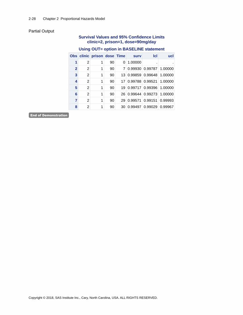
2-28 Chapter 2 Proportional Hazards Model
Copyright © 2018, SAS Institute Inc., Cary, North Carolina, USA. ALL RIGHTS RESERVED.
Partial Output
Survival Values and 95% Confidence Limits clinic=2, prison=1, dose=90mg/day
Using OUT= option in BASELINE statement
Obs clinic prison dose Time surv lcl ucl
1 2 1 90 0 1.00000 . .
2 2 1 90 7 0.99930 0.99787 1.00000
3 2 1 90 13 0.99859 0.99648 1.00000
4 2 1 90 17 0.99788 0.99521 1.00000
5 2 1 90 19 0.99717 0.99396 1.00000
6 2 1 90 26 0.99644 0.99273 1.00000
7 2 1 90 29 0.99571 0.99151 0.99993
8 2 1 90 30 0.99497 0.99029 0.99967

2.2 Chapter Summary 2-29
Copyright © 2018, SAS Institute Inc., Cary, North Carolina, USA. ALL RIGHTS RESERVED.
2.2 Chapter Summary
A common objective in survival analysis is to build a model that describes the relationship between the distribution of survival times and the explanatory variables. In survival models, the hazard function is the outcome the model tries to describe. In many situations, either the true form of the hazard function is unknown or it is so complex that the parametric distributions do not adequately describe it. However, the Cox proportional hazards model makes no assumptions regarding the nature of the hazard function. The model is very popular because it provides the primary information desired from a survival analysis, hazard ratios, and adjusted survival curves.
General form of the PHREG procedure:
PROC PHREG DATA=SAS-data-set <options>; CLASS variable <(options)><...variable <(options)>></options>; MODEL response<*censor(list)>=predictors </options>; STRATA variable<(list)><…variable<(list)>> </options>; CONTRAST <'label'>effect values<,.., effect values> </options>; ASSESS keyword </options>; HAZARDRATIO <'label'> variable </options>; WEIGHT variable</option; <label:> TEST equation1 <,..., equationk> < /options>; BASELINE <OUT=SAS data set> <COVARIATES=SAS-data-set> <keyword=name…keyword=name> </options>; OUTPUT <OUT=SAS-data-set> <keyword=name…keyword=name> </options>; <programming statements> RUN;

2-30 Chapter 2 Proportional Hazards Model
Copyright © 2018, SAS Institute Inc., Cary, North Carolina, USA. ALL RIGHTS RESERVED.

Appendix A References
A.1 References ........................................................................................................................... A-3

A-2 Appendix A References
Copyright © 2018, SAS Institute Inc., Cary, North Carolina, USA. ALL RIGHTS RESERVED.

A.1 References A-3
Copyright © 2018, SAS Institute Inc., Cary, North Carolina, USA. ALL RIGHTS RESERVED.
A.1 References
1. Allison, P. (2010), Survival Analysis Using the SAS System: A Practical Guide, Cary, NC: SAS Institute Inc.
2. Borgan, Ø. and Liestøl, K. (1990), “A Note on Confidence Interval and Bands for the Survival Curves Based on Transformations,” Scandinavian Journal of Statistics, 18: 35-41.
3. Cantor, A. (1997), Extending SAS Survival Analysis Techniques for Medical Research, Cary, NC: SAS Institute Inc.
4. Caplehorn, J., et al. (1991), “Methadone Dosage and Retention of Patients in Maintenance Treatment,” Medical Journal of Australia, 154: 195-199.
5. Chatfield, C. (1995), “Model Uncertainty, Data Mining and Statistical Inference," Journal of the Royal Statistical Society, 158: 419-466.
6. Cox, D.R. (1972), “Regression Models and Life Tables” (with discussion), Journal of the Royal Statistical Society, B34: 187-220.
7. Derksen, S. and Keselman, H.J. (1992), “Backward, Forward, and Stepwise Automated Subset Selection Algorithms: Frequency of Obtaining Authentic and Noise Variables,” British Journal of Mathematical and Statistical Psychology, 45: 265-282.
8. Freedman, D.A. (1983), “A Note on Screening Regression Equations,” The American Statistician, 37: 152-155.
9. Furnival, G.M. and Wilson, R.W. (1974), “Regressions by Leaps and Bounds,” Technometrics, 16: 499-511.
10. Grambsch, P.M., Therneau, T.M., and Fleming, T.R. (1995), “Diagnostic Plots to Reveal Functional Form for Covariates in Multiplicative Intensity Models,” Biometrics, 51: 1469-1482.
11. Grønnesby, J.K. and Borgan, Ø. (1996), “A Method for Checking Regression Models in Survival Analysis based on the Risk Score,” Lifetime Data Analysis, 2: 315-328.
12. Hall, W.J. and Wellner, J.A. (1980), “Confidence Bands for a Survival Curve for Censored Data,” Biometrika 69.
13. Harrell, F.E., Lee, K.L., and Mark, D.B. (1996), “Tutorial in Biostatistics Multivariable Prognostic Models: Issues in Developing Models, Evaluating Assumptions and Adequacy, and Measuring and Reducing Errors,” Statistics in Medicine, 15: 361-387.
14. Harrell, F.E. (1997), Predicting Outcomes: Applied Survival Analysis and Logistic Regression, Charlottesville, VA: School of Medicine, University of Virginia.
15. Hosmer, D.W. and Lemeshow, S. (2004), Applied Logistic Regression, Hoboken, NJ: John Wiley & Sons.
16. Hosmer, D.W. and Lemeshow, S. (2008), Applied Survival Analysis: Regression Modeling of Time to Event Data, Hoboken, NJ: John Wiley & Sons.
17. Kalbfleisch, J.D. and Prentice, R.L. (2002), The Statistical Analysis of Failure Time Data, Hoboken, NJ: John Wiley & Sons.

A-4 Appendix A References
Copyright © 2018, SAS Institute Inc., Cary, North Carolina, USA. ALL RIGHTS RESERVED.
18. Kaplan, E. L. and Meier, P. (1958), “Nonparametric estimation from incomplete observations,” Journal of the American Statistical Association, 53 (282): 457–481
19. Klein, J.P. and Moeschberger, M.L. (2005), Survival Analysis: Techniques for Censored and Truncated Data, New York: Springer Science + Business Media, Inc.
20. Kleinbaum, D.G., Kupper, L.L., Muller, K.E., and Nizam, A. (2008), Applied Regression Analysis and Other Multivariable Methods, Belmont, CA: Thomson Higher Education.
21. Kleinbaum, D.G. and Klein, M. (2005), Survival Analysis: A Self-Learning Text, New York: Springer Science + Business Media, Inc.
22. Liang, K.Y. and Zeger, S.L. (1986), “Longitudinal Data Analysis, using Generalized Linear Models,” Biometrika, 73: 13-22.
23. Lin, D.Y. and Wei, L.J. (1989), “The Robust Inference for the Cox Proportional Hazards Model,” Journal of the American Statistical Association, 84: 1074-1078.
24. Mallows, C.L. (1973), “Some Comments on Cp," Technometrics, 15: 661-675.
25. Mantel, M., Bohidar, N.R., and Ciminera, J. (1977), “Mantel-Haenszel analysis of litter-matched time-to-response data," Cancer Research, 37: 3863-3868.
26. May, S. and Hosmer, D.W. (1998), “A Simplified Method for Calculating a Goodness-of-Fit Test for the Proportional Hazards Model,” Lifetime Data Analysis, 4: 109-120.
27. Meeker, W.Q. and Escobar, L.A. (1998), Statistical Methods for Reliability Data, New York: John Wiley & Sons.
28. Prentice, R.L., Williams, J., and Peterson, A.V. (1981), “On the regression analysis of multivariate failure time data," Biometrika, 68: 373-379.
29. Raftery, A.E. (1995), “Bayesian Model Selection in Social Research," Sociological Methodology.
30. Ramlau-Hansen, H. (1983), “Smoothing Counting Process Intensities by Means of Kernel Functions," The Annals of Statistics, 11: 453-466.
31. Rothman, K.J. (1986), Modern Epidemiology, Boston: Little, Brown and Company.
32. SAS Institute Inc. (2011), SAS/STAT User’s Guide, Version 9.3, Cary, NC: SAS Institute Inc.
33. Scheffé, H. (1953), “A Method for Judging all Contrasts in the Analysis of Variance,” Biometrika, 40:87-104.
34. Schoenfeld, D. (1982), “Partial Residuals for the Proportional Hazards Regression Model," Biometrika, 69: 239-241.
35. Therneau, T.M., Grambsch, P.M., and Fleming, T.R. (1990), “Martingale-Based Residuals and Survival Models,” Biometrika, 77: 147-160.
36. Walker, G.A. (2008), Common Statistical Methods for Clinical Research with SAS Examples, Cary, NC: SAS Institute Inc.
37. Wei, L.J., Lin, D.Y., and Weissfeld (1989), “Regression analysis of multivariate incomplete failure time data by modeling marginal distributions,” Journal of the American Statistical Association, 84: 1065-1073.