CONTROL ENGINEERING LABORATORY

PROCESS CONTROL TOOL FOR A PRODUCTION LINE AT NOKIA

Sébastien Gebus

Report A No 13, December 2000

University of Oulu Department of Process and Environmental Engineering Control Engineering Laboratory Report A No 13, December 2000

PROCESS CONTROL TOOL FOR A PRODUCTION LINE AT NOKIA

Sébastien Gebus

Control Engineering Laboratory,

Department of Process and Environmental Engineering, University of Oulu

Linnanmaa, FIN-90014 University of Oulu, Finland

Abstract This report describes the application of Statistical Process Control (SPC) to improve the quality of manufacturing at Nokia. The production lines concerned in this study are modeled by a succession of placement machines, which are placing components on Printed Circuit Boards (PCB) used in internet broadband systems, and an optical control system measuring the position of each component. History and basic concept of SPC are reviewed using SPC PC IV as an example software tool. Combining SPC PC IV with intelligent systems was tested. Special requirements of the production system at Nokia are difficult for standard SPC techniques: small lot size, inspection programs not tuned up, not enough reliable data, etc. The approach described here is slightly different to the traditional SPC: only the main features of SPC have been used. The new Process Control Tool moves the process control towards active handling of the data. The tool is currently tested, and according to the preliminary results, improvement on following areas can be seen: better understanding of the process and its problems, faster response and in some cases even anticipated response, greater interest of the line workers who will have an active role in quality assurance. The Process Control Tool will be integrated as a part of the production line. The structure of the program makes different upgrades easy to implement.

Keywords: statistical process control, electronics manufacturing. ISBN 951-42-5870-3 University of Oulu ISSN 1238-9390 Department of Process and Environmental ISBN 951-42-7508-X (PDF) Engineering

Control Engineering Laboratory PL 4300

FIN-90014 University of Oulu

Table of Contents

1. INTRODUCTION .............................................................................................................. 4 2. STATISTICAL PROCESS CONTROL.............................................................................. 5

2.1 Some History .............................................................................................................. 5 2.2 Basic SPC concepts ................................................................................................... 6 2.3 SPC PC IV.................................................................................................................. 7

2.3.1 Features............................................................................................................... 7 2.3.2 Linking SPC PC IV with other systems............................................................... 10 2.3.3 Conclusion about SPC PC IV............................................................................. 10

3. DESCRIPTION OF THE PRODUCTION LINE ............................................................... 11 4. A GLOBAL AND FUNCTIONAL APPROACH WITH SADT (OR IDEF) METHOD......... 12 5. THE PREVIOUS PROCESS CONTROL TOOL ............................................................. 14

5.1 Description................................................................................................................ 14 5.1.1 System entities................................................................................................... 14 The previous system was mainly composed of the following entities: ............................ 14 5.1.2 System operation ............................................................................................... 15

5.2 Major problems encountered .................................................................................... 16 6. THE NEW PROCESS CONTROL TOOL ....................................................................... 17

6.1 Concept .................................................................................................................... 17 6.2 Major improvements ................................................................................................. 18

6.2.1 Database............................................................................................................ 18 6.2.2 Indatrans ............................................................................................................ 18 6.2.3 AQUA................................................................................................................. 19 6.2.4 Dipos.................................................................................................................. 24

7. PRELIMINARY RESULTS OF THE NEW SYSTEM....................................................... 25 8. CONCLUSIONS ............................................................................................................. 26 REFERENCES ...................................................................................................................... 27 ACKNOWLEDGEMENT ........................................................................................................ 27

4

1. INTRODUCTION

Statistical Process Control (SPC) is a toolkit, which plays an integral part in any system, designed to improve the quality of a process's outputs. It has to fulfill different tasks:

• = monitoring performance of a process by estimating its inputs and outputs against pre-determined standards,

• = interpreting the data provided by the monitoring to estimate effectiveness of the process, • = deciding upon and taking the appropriate action to:

o improve the process performance as a whole, o remove a problem adversely affecting the performance.

The initial idea was to use the results of a statistical analysis to get information about the system and to make corrections. But very early it became clear that it would be very difficult to implement this kind of function as an additional entity in the existing system. The current system was already complex enough since a part of the functions were made by other programs.

History and basic concept of SPC are reviewed using SPC PC IV as an example software tool. Clearly SPC tools should be combined with intelligent systems but an important question is how to do it.

Special requirements of the production system at Nokia are also handled. The nature of the system is difficult for standard SPC techniques: small lot size, inspection programs not tuned up, not enough reliable data, etc. The information obtained by this statistical analysis would have been uncertain and useless. Therefore, the approach described here is slightly different to the traditional SPC: only the main features of SPC have been used.

This report concentrates on main objectives and functions of the Process Control Tool. The main goal is to develop additional SPC based tools for integrating the present systems. For this purpose the problems encountered in the existing systems are addressed. The new tool moves the process control towards active handling of the data.

5

2. STATISTICAL PROCESS CONTROL

2.1 Some History

Statistical Process Control (SPC) monitors the process to reduce (but not remove) the need for inspection of every output. One objective of installing SPC is therefore to use a process control system that will focus on defect prevention rather than defect detection in order to have a quality assurance on the output without having to use a 100 percent inspection. But in this part we will not talk about all history of quality, otherwise we would have to go back to the Egyptians where architects were simply killed if the buildings were collapsing and the lodgers died. Now you know the reason of the use of very thick walls in Egyptian architecture. Let's better start at early part of this century when SPC was developed.

In the 1920's, Dr. Walter Shewhart, a statistician, was working in the laboratories of Bell Telephone Company in the USA. He was studying variability in the natural world, and was asked by Bell to apply the same techniques to find out why there was so much variability between the telephones they produced. Shewhart's research led him to the conclusion that every process displays variation, some processes display controlled variation while others display uncontrolled variation:

• = Controlled variation shows a stable and consistent pattern over time, and is therefore always present in the process. This variation is due to common causes affecting the process.

• = On the other hand, uncontrolled variation shows a pattern that changes over time, and which therefore means that the process itself is both inconsistent and unstable.

Without the actual data processing technologies (in other words the computers), Shewhart had to develop an easy handling method to monitor processes and identify the presence of these areas of uncontrolled variation, which he considered to be assignable causes of variation. Shewhart published his first Control Chart in 1924, and his book, "The Economic Control of Quality of Manufactured Product" in 1931. Unfortunately for both Shewhart and Western industry, his ideas were largely ignored in America and Europe where quality was not a priority because of the economic growth and the fact that the demand was still much bigger than the supply. However, Shewhart is not the most famous name when you are speaking about SPC. Another man has done much more to make SPC concept more widely known.

Dr. W. Edwards Deming has worked with Shewhart at Bell. In 1938 he arranged for Shewhart to give a series of lectures on the industrial application of statistics. But the great jump forward for both Deming and SPC came after the war: in 1947, Deming was asked to go to Japan and help the Government prepare for a census. There he met several statisticians and businessmen deeply concerned about the state of their country's industrial base, which was in a shamble after the war. As everything was destroyed on this island, which was even without any natural resources, they could not waste a lot of energy and time by producing junk. Deming told them that they could become an important economic force by applying SPC to their manufacturing processes.

Three years later, in 1950, Deming was invited back to Japan to give a series of seminars on SPC to members of the Union of Japanese Scientists and Engineers (JUSE). At the first seminar, Dr. Ishikawa introduced Deming to 21 of the country's top industrialists, including the heads of Nissan, Sony, Toyota and Mitsubishi. The rest, as they say, is history.

6

2.2 Basic SPC concepts

Tampering, i.e. making modifications in the process because of false alarms before it has really shifted, is considered as a big problem in modern industries. Normal variability of the system can be taken for an exceptional shift or a mistake. Don’t forget that for a normal law for example, there are still 0,27 percent of the values that are not between the three sigmas limits. A modification in this case will have for effect to move the average value.

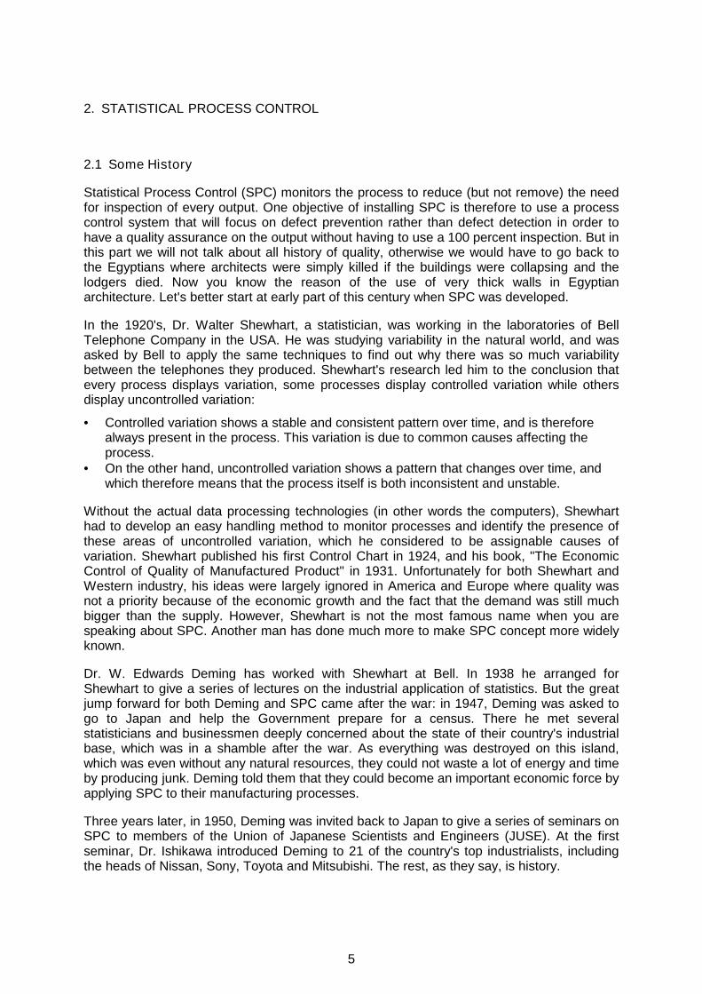
In fact, two factors can define a process: variation and accuracy, and commonly you should be in one of the four following cases shown in Figure 1.

Figure 1. Process types.

In these situations, the thing to do is first to adjust the parameters to have again the system under control, and then to try to reduce the variability. Completely on opposite of the tampering there is another rule: by reacting to the process and checking its outcome only at the end, it is not possible to establish how or where any problems occurred, or how the process could be improved. That’s why the three sigmas test is usually not enough to define when a problem has occurred or will occur. The most common run tests are the following:

1. check the points out of the 3 sigma limits 2. 9 consecutive points on the same side of the average value 3. 6 consecutive points increasing or decreasing 4. 14 consecutive points being alternatively over and under the average value 5. for 3 consecutive points, 2 of them are out of the 2 sigma limit 6. for 5 consecutive points, 4 of them are out of the 1 sigma limit 7. 15 points between the 1 sigma limit (stratification in sampling) 8. ... There can be a lot of other rules and you have to adapt them to your process in order to have the good information without having too many false alarms. For this project for example, none of the previous rules has been used.

Process in control and capable

Process not in control and not capable

Process capable but not in control

Process in control but not capable

7

One last rule in SPC implementation is probably the most important: frontline workers know more about his job than anyone else does. This has to be kept in mind before trying to adjust some parameters.

When applied correctly, SPC contributes:

1. achieving consistency in outputs (economic optimum required by the customer) 2. improving the predictability of process behaviour 3. achieving an environment of continuous improvement 4. reducing the cost of quality 5. delighting the customer (which is after all the final quality goal)

2.3 SPC PC IV

SPC PC IV is a widely known SPC software tool which includes both basic and advanced features of SPC. I have studied the basic features and how it would be possible to use them in a real time feedback.

2.3.1 Features

Basic options of this software are to draw some nice and colourful control charts and to give some statistical information like Cpk. But to use this software some mathematical bases are needed to interprete these values and to adjust parameters. For curve fit selection, I could notice that the best-fit selection (Johnson) is not always the one, which gives the best Kolmogorov-Smirnoff (K-S) parameter. And I am not even sure if the Ki square parameter is checked. The Best Fit is the default selection but changing the curve fit selection changes the approximation of the distribution which can have a big influence on the statistical results. Here appears then already one of the biggest limitation of this software due to the nature of the process. The statistical analysis is based on the approximation of the process, but this process is not stable and the data not very reliable. So if the approximation is wrong then the analysis is wrong.

The choice of a control chart depends on the type of data and on what you want to get for information. There are different possibilities for making control charts.

Attribute Charts

Np-chart is for monitoring the number of times a condition occurs. The samples have a constant size and can either have or not this condition.

p-chart is for monitoring the percent of samples having this condition. The samples have a variable size and can either have or not this condition.

c-chart is for monitoring the number of times a condition occurs. The samples have a constant size and can have more than one instance of this condition.

u-chart is for monitoring the percent of samples having this condition. The samples have a variable size and can have more than one instance of this condition.

These charts are usually used to count the number of errors without taking care of the importance of these errors

8

Pareto charts

Pareto charts are used to prioritise problems. Data must be cumulative (counts or costs) and only attributes.

Check Sheet

Check sheets are used to monitor the frequency of occurrence of events. Like Pareto charts, they can be used to prioritise problems.

X-bar & Range charts

These charts are only for variable data, which means that quantitative and continuous measurements are requred. These are used when you are able to collect data in subgroups (from 2 to 10 subgroups). Each subgroup represents a snapshot of the process at a given time.

If there is a bigger amount of subgroups, a sigma chart should be used to calculate the variation. Control limits on X-bar chart depend on the variation. This means that there is no sense to try to analyse the X-bar chart if the range chart is out of control.

X-bar & Sigma charts

These charts are the same as the X-bar & range charts but for a bigger amount of subgroups. In this case sigma gives a better approximation of the variation.

Individual X & Moving Range chart

These charts are used when you cannot group measurements into subgroups.

Process capability charts

These charts answer the question: can we consistently meet customer requirements?

This is only a prediction, and it is only possible to predict something if the process is stable and under control. If there are multiple peaks on the histogram, you should try to find out the reason. Commonly a process is considered to be good if Cpk > 1.33.

Scatter Diagrams

The scatter diagram examines the relations between two variables. It can show if this relation is strong or week, but it cannot explain the relation. If we find a relation between two variables, we can use one of these variables instead of the other.

On the diagram, a relation will be represented by a curve.

Autocorrelation charts (ACF)

These charts can show dependence between the data. You can for example find some cyclic data. In order to use these charts, the observations must be independent.

9

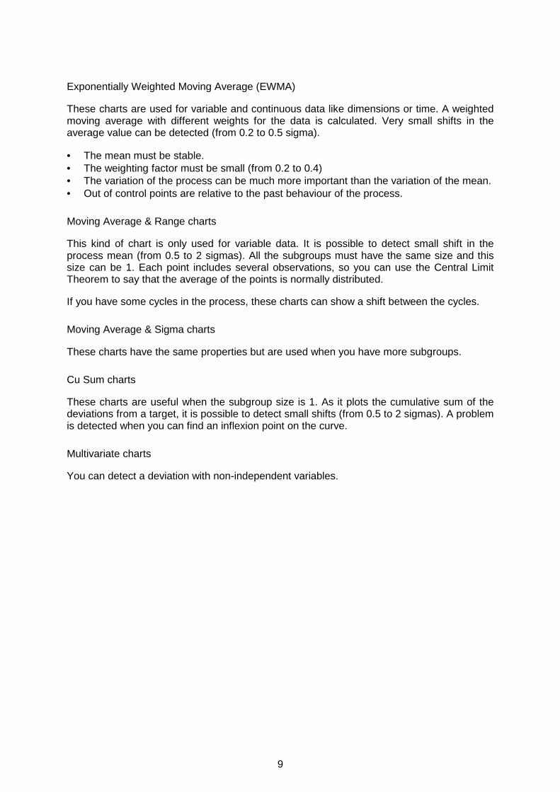
Exponentially Weighted Moving Average (EWMA)

These charts are used for variable and continuous data like dimensions or time. A weighted moving average with different weights for the data is calculated. Very small shifts in the average value can be detected (from 0.2 to 0.5 sigma).

• = The mean must be stable. • = The weighting factor must be small (from 0.2 to 0.4) • = The variation of the process can be much more important than the variation of the mean. • = Out of control points are relative to the past behaviour of the process.

Moving Average & Range charts

This kind of chart is only used for variable data. It is possible to detect small shift in the process mean (from 0.5 to 2 sigmas). All the subgroups must have the same size and this size can be 1. Each point includes several observations, so you can use the Central Limit Theorem to say that the average of the points is normally distributed.

If you have some cycles in the process, these charts can show a shift between the cycles.

Moving Average & Sigma charts

These charts have the same properties but are used when you have more subgroups.

Cu Sum charts

These charts are useful when the subgroup size is 1. As it plots the cumulative sum of the deviations from a target, it is possible to detect small shifts (from 0.5 to 2 sigmas). A problem is detected when you can find an inflexion point on the curve.

Multivariate charts

You can detect a deviation with non-independent variables.

10

2.3.2 Linking SPC PC IV with other systems

An important benefit of the SPC PC IV software is the possibility to create links with a database. However, this feature is not as developed as has first been thought. The lack of documentation for this kind of links shows that the feature has been added very recently and that the main aim of the software is not to work online and in real time with the process.

As far as DDE links are concerned, I have studied the possibilities of links between SPC PC IV, Excel and Matlab. Even if SPC PC IV is a powerful tool for analysing data, it does not include for example fuzzy tools and that's where the fuzzy toolbox of Matlab can be very useful. However, these links are not more detailed than the links with the database. You don't even know for example that SPC PC IV software is called under windows "SPCWIN" (this information is needed to identify the software for creating the link). It also seems to offer quite limited possibilities. To create a DDE link between two files, both softwares must be running and these files must be open, then it is possible to exchange and update data but only in very limited fields. With SPC PC IV you can only have access to the data sheet but it seems to be impossible to have access to the parameter window. It is possible to modify and update data in real time but not for example to change the control limits.

2.3.3 Conclusion about SPC PC IV

According to the tests, SPC PC IV is not optimised for an online and real time use with a database or another software. It can be used to analyse "manually" history data in order to make a static analysis of the former data to eventually predict the future situation of the process. It is impossible to have a real time or even a fast feedback about the current situation.

Like other SPC softwares SPC PC IV is designed for mass production systems. Our case requires additional features. The analysis is base on approximating the production with a mathematical model. This model will be erroneous if the process is not stable enough and the data not reliable. The conclusions made with such a model would be even worse.

SPC is a powerful tool if it is not misused and if you are in an adequate situation. So let's then describe the situation at Nokia and the real need in term of process control. If a statistical analyse is difficult to use, we will have to find a different way to get the information.

11

3. DESCRIPTION OF THE PRODUCTION LINE

A simple model of the production line is a succession of placement machines and at the end of them an optical control system that measures the position in X and Y direction for each component. Actually, the control system is not at the end of the production line, because we should not forget that after being controlled, there is a line worker who has to make corrections. He gets the information for making correction from two ways:

• = A visual inspection of the PCB. The experience of the line worker is very important for detecting problems. But it becomes more and more difficult for him because we are not in a situation of mass production. The number of PCB and their complexity is even increasing with time. And you can have up to several hundreds of components per PCB.

• = The control system gives information about missing or misplaced components. There are a lot of false alarms due to imprecision in the measurements.

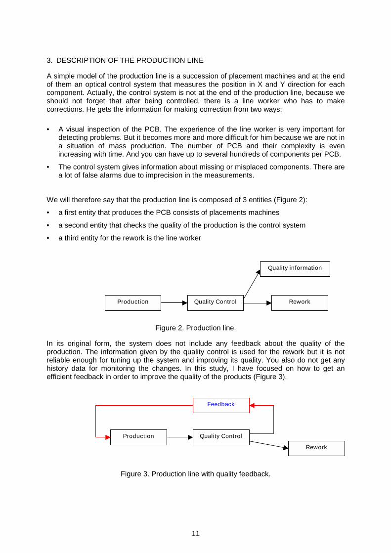
We will therefore say that the production line is composed of 3 entities (Figure 2):

• = a first entity that produces the PCB consists of placements machines

• = a second entity that checks the quality of the production is the control system

• = a third entity for the rework is the line worker

Figure 2. Production line.

In its original form, the system does not include any feedback about the quality of the production. The information given by the quality control is used for the rework but it is not reliable enough for tuning up the system and improving its quality. You also do not get any history data for monitoring the changes. In this study, I have focused on how to get an efficient feedback in order to improve the quality of the products (Figure 3).

Figure 3. Production line with quality feedback.

Production Rework Quality Control

Feedback

Production

Rework

Quality Control

Quality information

12

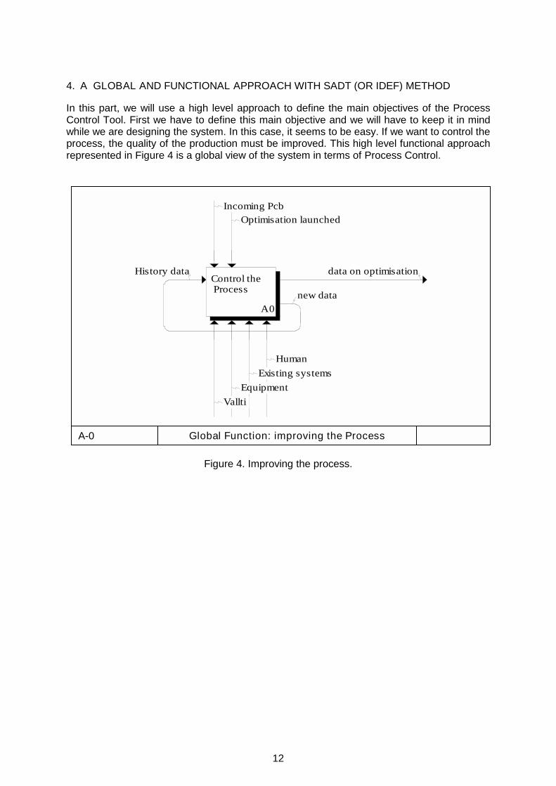
4. A GLOBAL AND FUNCTIONAL APPROACH WITH SADT (OR IDEF) METHOD

In this part, we will use a high level approach to define the main objectives of the Process Control Tool. First we have to define this main objective and we will have to keep it in mind while we are designing the system. In this case, it seems to be easy. If we want to control the process, the quality of the production must be improved. This high level functional approach represented in Figure 4 is a global view of the system in terms of Process Control.

Figure 4. Improving the process.

A-0 Global Function: improving the Process

Control the Process

A0new data

data on optimisationHistory data

Vallti

Equipment

Existing systems

Incoming PcbOptimisation launched

Human

13

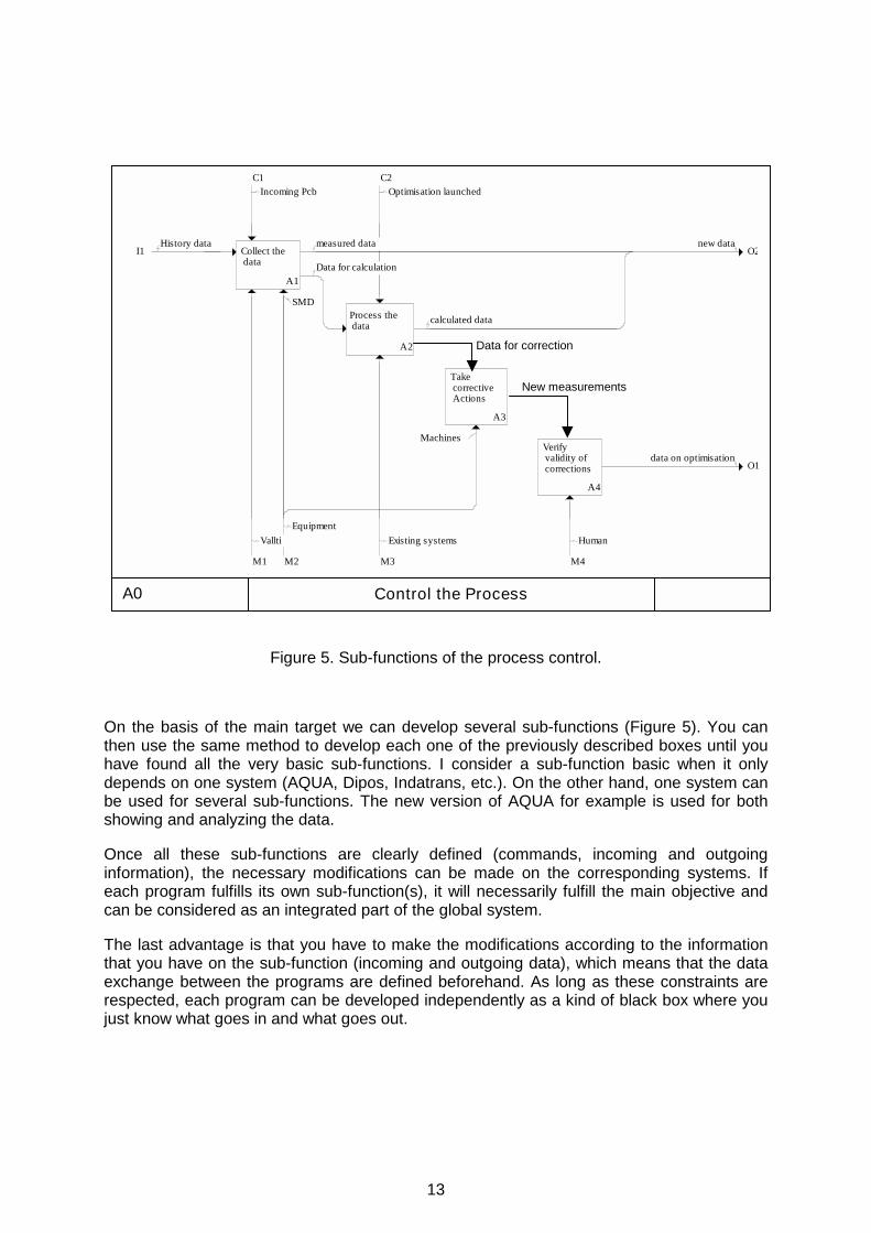
Figure 5. Sub-functions of the process control.

On the basis of the main target we can develop several sub-functions (Figure 5). You can then use the same method to develop each one of the previously described boxes until you have found all the very basic sub-functions. I consider a sub-function basic when it only depends on one system (AQUA, Dipos, Indatrans, etc.). On the other hand, one system can be used for several sub-functions. The new version of AQUA for example is used for both showing and analyzing the data.

Once all these sub-functions are clearly defined (commands, incoming and outgoing information), the necessary modifications can be made on the corresponding systems. If each program fulfills its own sub-function(s), it will necessarily fulfill the main objective and can be considered as an integrated part of the global system.

The last advantage is that you have to make the modifications according to the information that you have on the sub-function (incoming and outgoing data), which means that the data exchange between the programs are defined beforehand. As long as these constraints are respected, each program can be developed independently as a kind of black box where you just know what goes in and what goes out.

A0 Control the Process

O1

I1 O2

M4

C2

M3M2

C1

M1

Verify validity of corrections

A4

Take corrective Actions

A3

Process the data

A2

Collect the data

A1

data on optimisation

calculated data

History data

Data for calculation

measured data new data

Human

Machines

Optimisation launched

Existing systems

Incoming Pcb

Vallti

Equipment

SMD

Data for correction

New measurements

14

5. THE PREVIOUS PROCESS CONTROL TOOL

5.1 Description

Various systems were already present on the production line but they were in their previous version unable to monitor and control the process. The main reason for this was that they have been designed independently and were therefore also working independently. Each system was manipulating a very specific set of data in order to fulfill a very specific and local objective. These programs have been optimised in that way. And contrary to what has been said before and what should have been done, these local objectives were also independent.

5.1.1 System entities

The previous system was mainly composed of the following entities:

Indatrans was collecting the measurements from the SMD inspection machine. The data were compressed and only average, minimum, maximum and threshold values for each material code were kept and sent to database. A material code represents one type of component for one side of the PCB. In some cases, one material code represents one component, but it can also represent many more (even 100 or more).

AQUA has been used for showing the data on charts. A time limit was defined and all the data for a selected product (PCB, side and material code) corresponding for the time limit were shown on charts.

Dipos gives a picture of the PCB with all the components. It could be used to locate the components but the necessary information was difficult to find, i.e. several manual operations were needed to determine the serial number, the component name, etc.

VALTTI is the global database. The three other entities had specific tables in VALTTI.

15

5.1.2 System operation

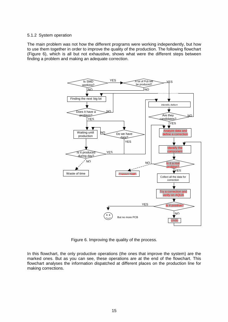
The main problem was not how the different programs were working independently, but how to use them together in order to improve the quality of the production. The following flowchart (Figure 6), which is all but not exhaustive, shows what were the different steps between finding a problem and making an adequate correction.

Figure 6. Improving the quality of the process.

In this flowchart, the only productive operations (the ones that improve the system) are the marked ones. But as you can see, these operations are at the end of the flowchart. This flowchart analyses the information dispatched at different places on the production line for making corrections.

Is SMD working?

Is it a real problem?

A lot of Pcb will be produced?

Is it produced during day?

Do we have data?

Does it have a problem?

Is it positive?

Are they candidates?

Finding the next big lot

Waiting until production

Waste of time

Identify defect

Analyze data and define a correction

Identify the component

Correct SMDCollect all the data for

correction

Try a correction and verify on AQUA

But no more PCBUndo

YES YES

YES

YES

YES

YES

YES

YES

NO NO

NONO

NO

NONO

NO

16

A lot of time is wasted for finding a product that could have a defect simply because this kind of product has to fulfill at least the following conditions:

• = It will be produced soon or at least during the working time of the programmer who has to make the corrections.

• = A control program must be existing for this type of product (with the good release) • = Data must be available if you want to make any analysis (20 values at least) • = The amount of PCB that will be produced must be big enough to verify the

effectiveness of the corrections. These conditions are necessary even before trying to analyse the data for a specific PCB. With the previous system, everything had to be done manually and a lot of time was wasted for usually arriving at the conclusion that at least one of these conditions was not fulfilled. The most common case was that when a defect was finally clearly identified (what component, what kind of defect and what is the correction), this PCB was not anymore produced or only few units were produced before starting a different lot.

That is a reason why a functional approach has been used. The first part of the flowchart is also composed of necessary functions and one target of the new Process Control Tool was to assign these functions to one of the existing programs. Another target was to speed up the second part of the flowchart by making an intelligent analysis of the data and by providing the useful information for tuning up the production line.

5.2 Major problems encountered

Compression of the data: The data sent to VALTTI were not raw data but compressed data. The choice of the compression method resulted in a loss of almost all the information that is needed for detecting and correcting any problem:

• = This compression method generated theshold errors when some components for one material code had a different orientation. Only the thresholds for the first component were kept, which means that rotated components were checked with wrong thresholds.

• = The information that was needed for making corrections was absent from database.

Identification of a problem: The information (mainly charts) provided by AQUA was useless. It was only showing the data sent by Indatrans to VALTTI, and these data were not reliable because of the compression method. The basic function for AQUA, which should have been to make it easy to detect and to identify a problem, was not in the program and AQUA provided only "defect candidates". Once a problem was found, it also did not give any information about the incriminated component.

Analysis of the data: In order to have more information about defective products (on a component level instead of a material code level for example), the only way was to get the text files containing the measurements made by the Automatic Optical Inspection (AOI). These files had to be analysed with Excel to find the type of defect. Such an operation takes a lot of time, and was often useless because only few "defect candidates" were finally real defects.

Data availability: Database contained data only for a specific time period (usually last 2 weeks). This solution can be used in a mass production system, but in our case it means that we have for some components hundreds of data points and for other ones nothing at all. In these conditions it was impossible to realise an effective and automatic analysis of the data, even when we had the data.

17

6. THE NEW PROCESS CONTROL TOOL

6.1 Concept

The main problems of using the existing system in the process control can be summarised in the following way: "We don't know what is happening on the production line and when finally we know it, it is too late to act". Now it is time to imagine and to design a new solution.

In order not to make too big structural changes, the main systems (Indatrans, AQUA and Dipos) have been kept, but some new features have been added by updating the old ones. Everything has also been made in the aim to control the process, which means obtaining a quick feedback about the production in order to make corrections.

The design process of this new system is following:

• = What are the different kinds of defects on the production line? This part needs a good understanding of the process. Answers can be given for example by the line workers. Major problems of the previous system have to be identified.

• = What kind of information do we need? If we want to control the process in an effective way, we need to have information about the production in a way that is easy to understand with some key parameters. The control system must be able to show precisely where is a problem (which component is shifted for example), how big is this problem (how big is the shift according to the threshold value) and it must give information for the correction that has to be made. Is it a trend or only a local defect? Which is the placement machine for this component?

• = What is the best way to show this information? Charts, tables, text files, etc.? The program itself has to be easy to use and to understand, that is why the amount of information available and the way to show it has to be adapted to what you want to do with them.

• = How can we obtain this information? In this part, we have to define what are the data that we have to collect and how these data become real information. For a shift for example, we just need to know the relative position of a component and the threshold value for this component and we can obtain an indication about the shift. Only this indication has to be shown to the user who wants to know if the component has a defect. However, more information has to be accessible for the correction, which sends us back to the previous point, "what to show and how to show it ?".

• = Where and how can we collect these data? That is the "physical" part of the production line. In other words, where and what kind of measurements do we need?

Practically it was not possible to make everything in this order, especially the last point is problematic. The existing system has always been kept in mind because the primary objective of this project was to control the process and not to re-design the production line. Therefore some allowances had to be made. But the concept is still going in the opposite way of what has been done for the previous system, which was:

• = building up a control system, • = saving some data to the database, • = showing these data on charts, • = asking ourselves what could be done with these charts.

18

6.2 Major improvements

Major improvements were done by updating the existing systems: data availability was addressed in handling of databases, data compression techniques of Indatrans were improved, monitoring and analysing functions were included to AQUA, and finally, locating the faulty components was done by integrating Dipos to the Process Control Tool.

6.2.1 Database

All the data necessary for the process control tool is now in a unique table, and only the data that are necessary are in this table. It means that with these data we are able to detect a defect and to make the correction.

Data availability

This problem has been solved and now for each component we have the 20 last values, whenever they have been produced. Of course old data are not very reliable but anyway better than no data at all. And we have also access to the date when the measurement has been made.

6.2.2 Indatrans

Indatrans is still responsible for compressing the data and sending them to database. It is also keeping it up by checking the size and suppressing the oldest lines when more than 20 values are stored. These 20 values are only an option. If in the future more values are needed, there is only a parameter to change for saving more than 20 values to database.

Data compression

A material code is composed of one or more identical components. The previous version of Indatrans was sending the average, the minimum and the maximum values for the measured positions of the components to the database. The threshold of the first component was used for all the following ones, even if some of them were rotated and had different thresholds. With the new version, only the average value has been kept (for making corrections). To solve the threshold problem, all other values are now standardised. Standard average, minimum and maximum have been calculated by using the measurements divided by their specific thresholds.

In order to have access to component level information, we have also saved the reference numbers of the components responsible for the maximum and the minimum values in each direction. It can be used to detect for example when a big variation in the data for a material code is due only to a few numbers of components.

The other stored information is used for the localisation of a component, e.g. serial number, to make corrections easier.

19

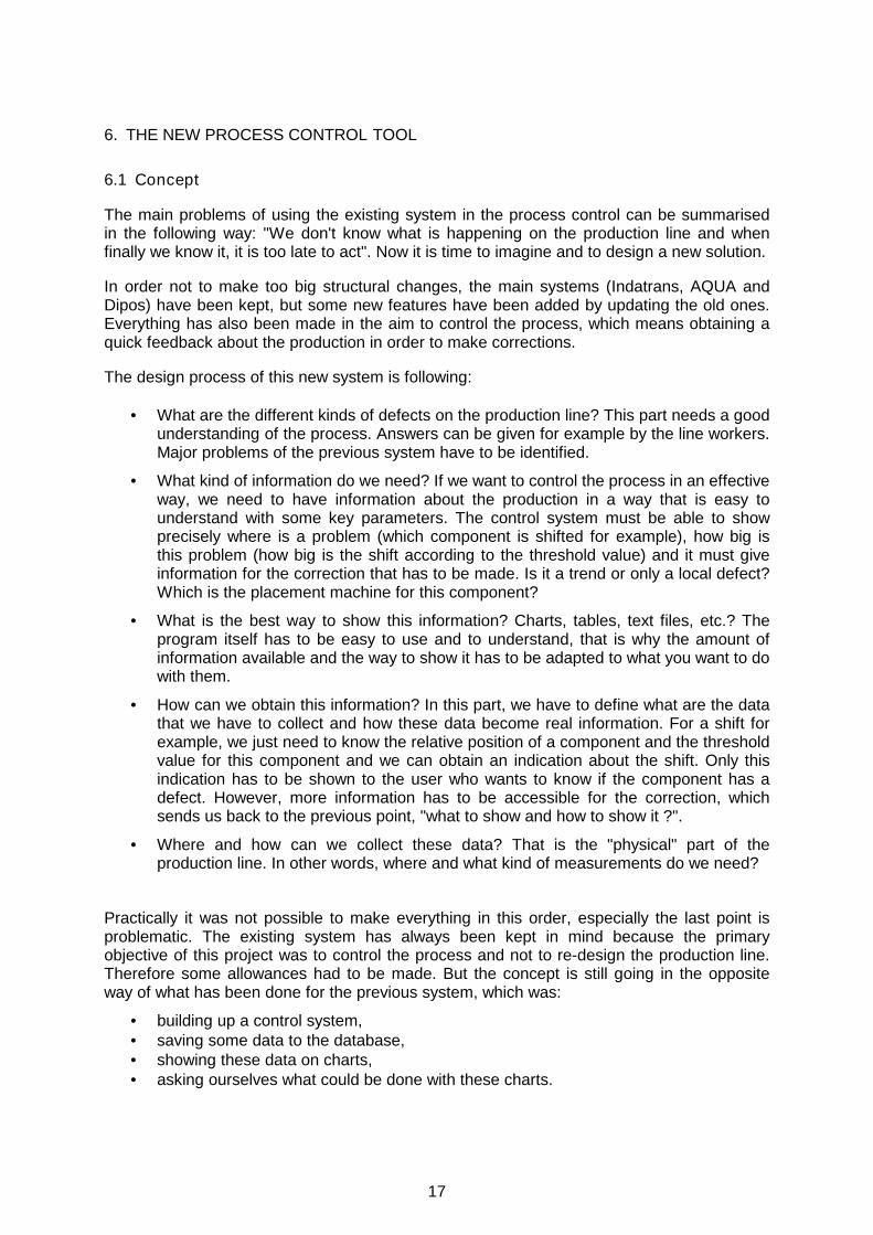
6.2.3 AQUA

AQUA has now two specific functions, a monitoring function and an analysing function. The presentation of the program has been improved and is very graphical as you can see on Figure 7. We will not see all the options in detail, but here is the description of these two functions.

Figure 7. Monitoring and analysing functions of AQUA.

Figure 1: AQUA main view.

20

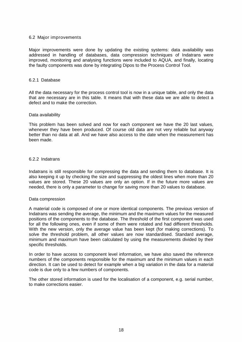
Monitoring function

The product identification bar (Figure 8) is used to select the product that you want to monitor.

Figure 8. Product identifier of the monitoring function.

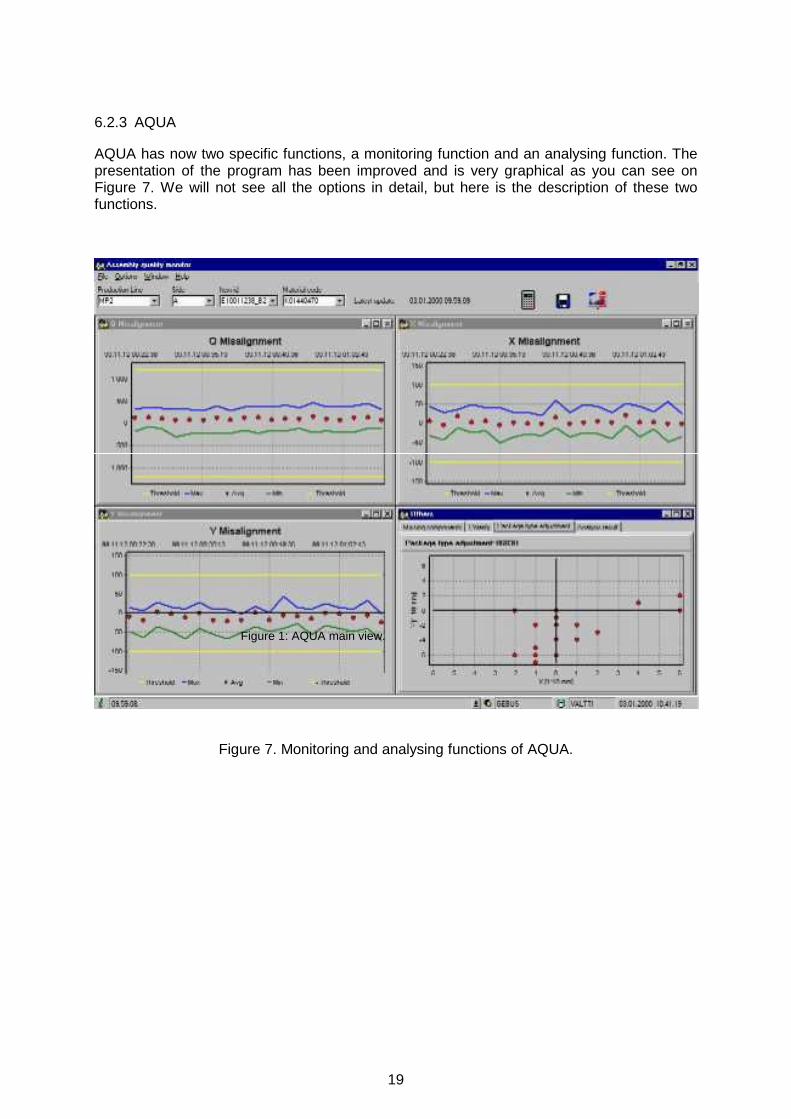
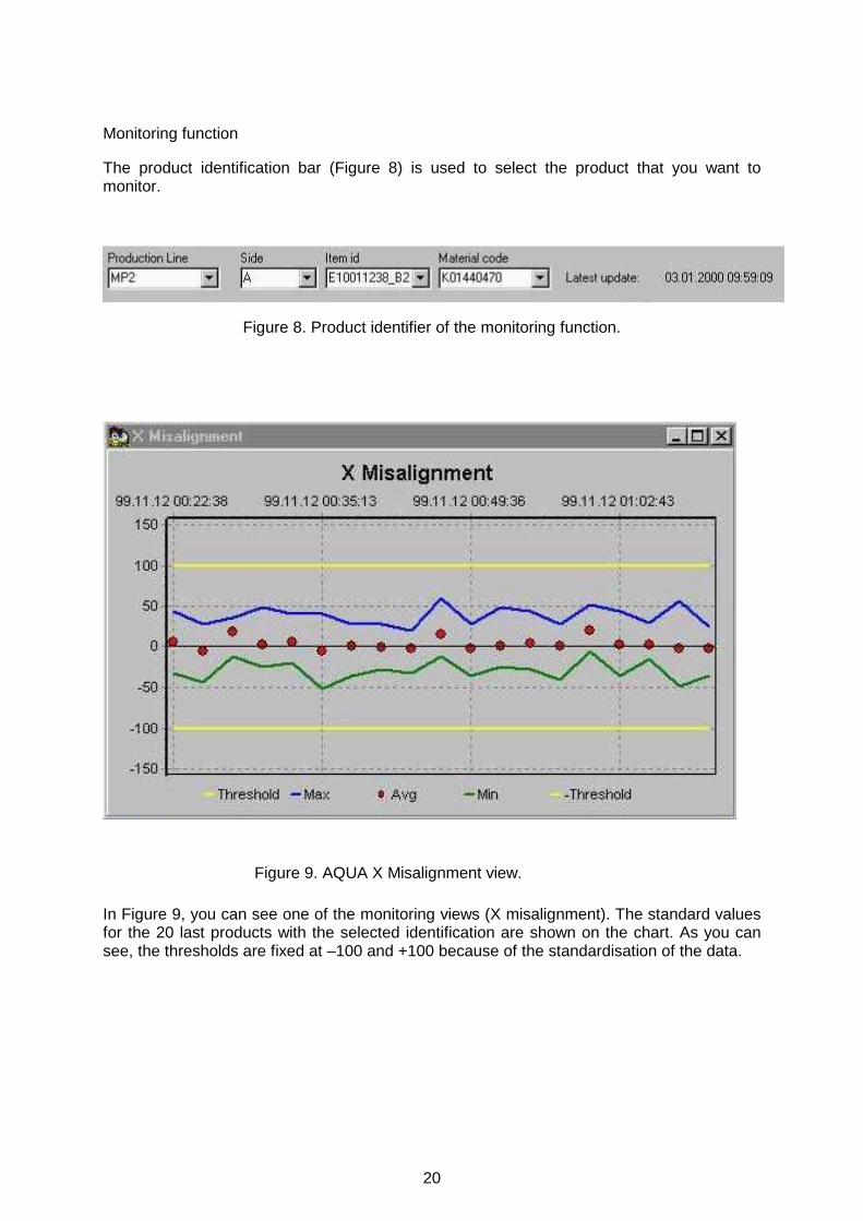
In Figure 9, you can see one of the monitoring views (X misalignment). The standard values for the 20 last products with the selected identification are shown on the chart. As you can see, the thresholds are fixed at –100 and +100 because of the standardisation of the data.

Figure 9. AQUA X Misalignment view.

21

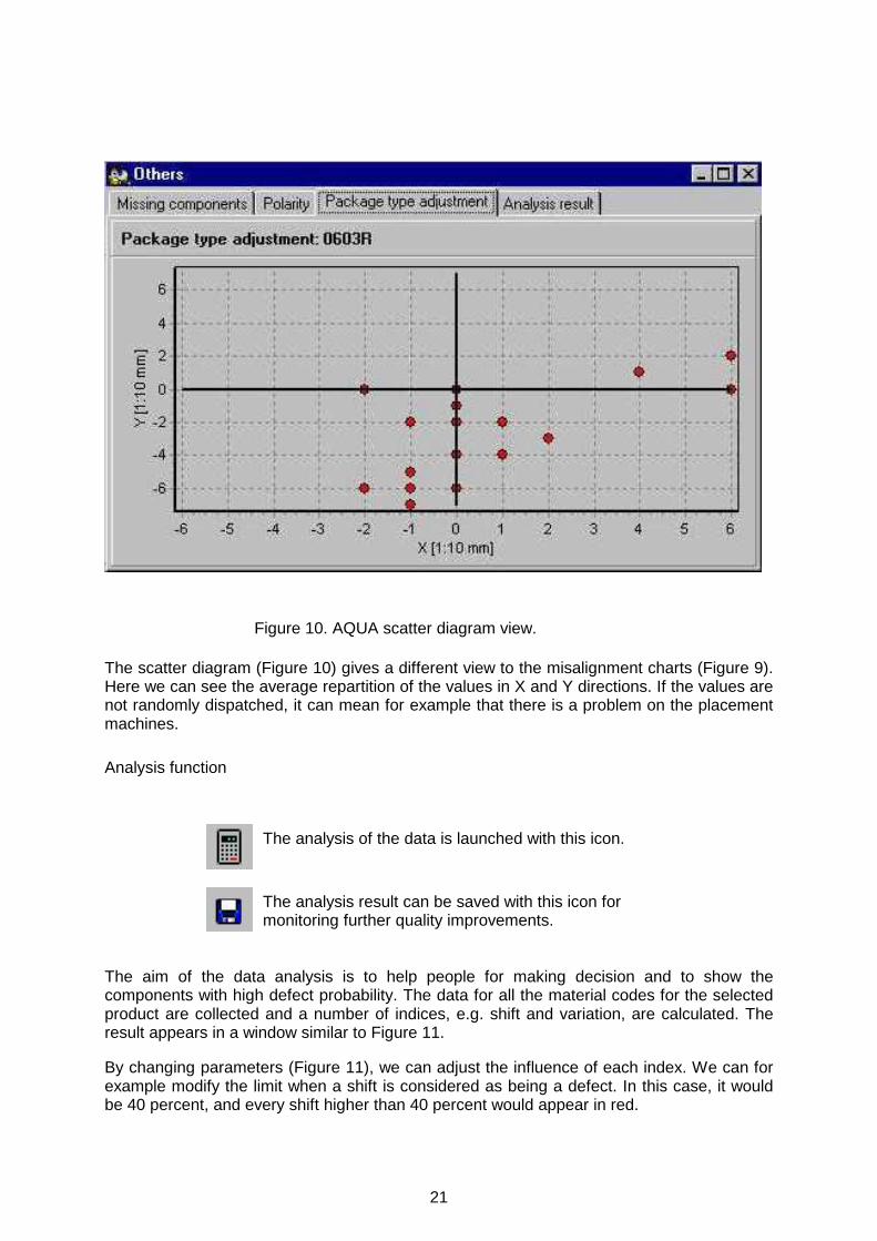
The scatter diagram (Figure 10) gives a different view to the misalignment charts (Figure 9). Here we can see the average repartition of the values in X and Y directions. If the values are not randomly dispatched, it can mean for example that there is a problem on the placement machines.

Analysis function

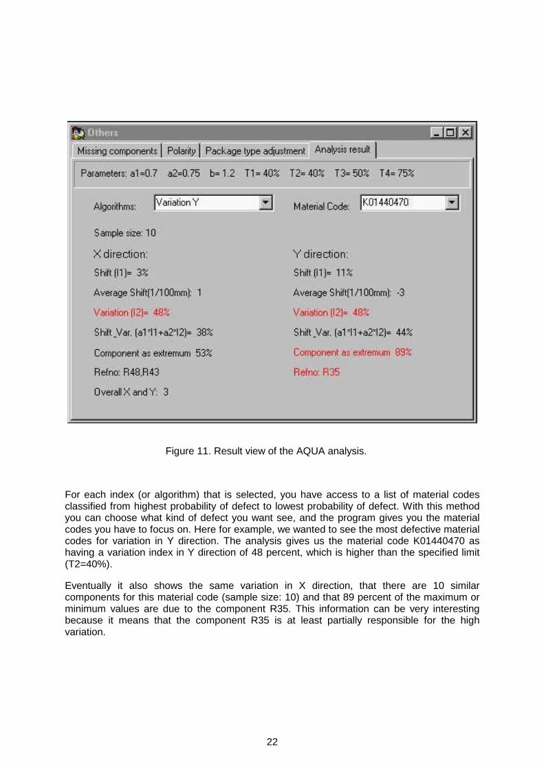
The aim of the data analysis is to help people for making decision and to show the components with high defect probability. The data for all the material codes for the selected product are collected and a number of indices, e.g. shift and variation, are calculated. The result appears in a window similar to Figure 11.

By changing parameters (Figure 11), we can adjust the influence of each index. We can for example modify the limit when a shift is considered as being a defect. In this case, it would be 40 percent, and every shift higher than 40 percent would appear in red.

Figure 10. AQUA scatter diagram view.

The analysis of the data is launched with this icon.

The analysis result can be saved with this icon for monitoring further quality improvements.

22

For each index (or algorithm) that is selected, you have access to a list of material codes classified from highest probability of defect to lowest probability of defect. With this method you can choose what kind of defect you want see, and the program gives you the material codes you have to focus on. Here for example, we wanted to see the most defective material codes for variation in Y direction. The analysis gives us the material code K01440470 as having a variation index in Y direction of 48 percent, which is higher than the specified limit (T2=40%).

Eventually it also shows the same variation in X direction, that there are 10 similar components for this material code (sample size: 10) and that 89 percent of the maximum or minimum values are due to the component R35. This information can be very interesting because it means that the component R35 is at least partially responsible for the high variation.

Figure 11. Result view of the AQUA analysis.

23

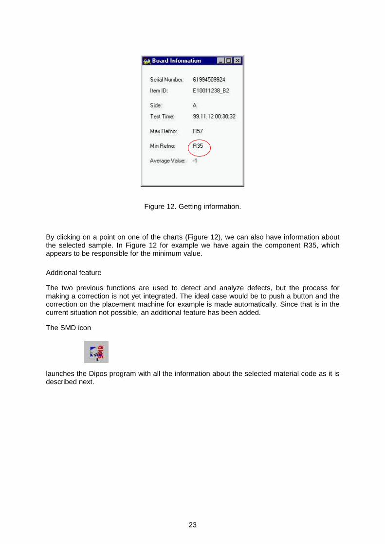
Figure 12. Getting information.

By clicking on a point on one of the charts (Figure 12), we can also have information about the selected sample. In Figure 12 for example we have again the component R35, which appears to be responsible for the minimum value.

Additional feature

The two previous functions are used to detect and analyze defects, but the process for making a correction is not yet integrated. The ideal case would be to push a button and the correction on the placement machine for example is made automatically. Since that is in the current situation not possible, an additional feature has been added.

The SMD icon

launches the Dipos program with all the information about the selected material code as it is described next.

24

6.2.4 Dipos

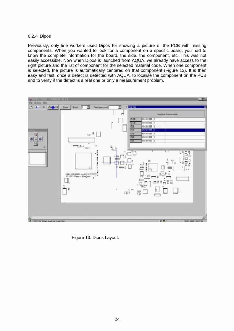
Previously, only line workers used Dipos for showing a picture of the PCB with missing components. When you wanted to look for a component on a specific board, you had to know the complete information for the board, the side, the component, etc. This was not easily accessible. Now when Dipos is launched from AQUA, we already have access to the right picture and the list of component for the selected material code. When one component is selected, the picture is automatically centered on that component (Figure 13). It is then easy and fast, once a defect is detected with AQUA, to localise the component on the PCB and to verify if the defect is a real one or only a measurement problem.

Figure 13. Dipos Layout.

25

7. PRELIMINARY RESULTS OF THE NEW SYSTEM

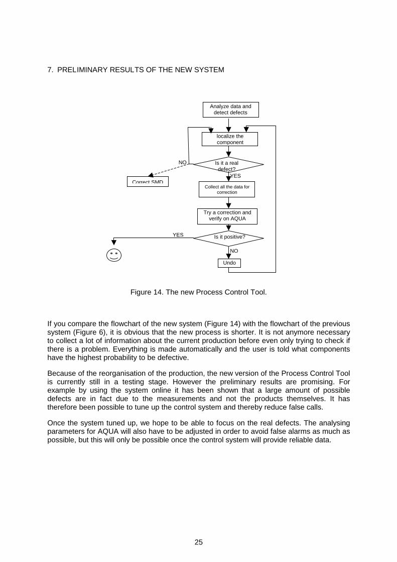
Figure 14. The new Process Control Tool.

If you compare the flowchart of the new system (Figure 14) with the flowchart of the previous system (Figure 6), it is obvious that the new process is shorter. It is not anymore necessary to collect a lot of information about the current production before even only trying to check if there is a problem. Everything is made automatically and the user is told what components have the highest probability to be defective.

Because of the reorganisation of the production, the new version of the Process Control Tool is currently still in a testing stage. However the preliminary results are promising. For example by using the system online it has been shown that a large amount of possible defects are in fact due to the measurements and not the products themselves. It has therefore been possible to tune up the control system and thereby reduce false calls.

Once the system tuned up, we hope to be able to focus on the real defects. The analysing parameters for AQUA will also have to be adjusted in order to avoid false alarms as much as possible, but this will only be possible once the control system will provide reliable data.

Is it a real defect?

Is it positive?

Analyze data and detect defects

localize the component

Correct SMDCollect all the data for

correction

Try a correction and verify on AQUA

Undo

YES

YES

NO

NO

26

8. CONCLUSIONS

Initially presented as a SPC project using Fuzzy Logic for taking decisions, we soon became short on adequate tools for this kind of work. SPC PC IV and Matlab were not adapted to the situation. SPC PC IV is for analysing history data, and Matlab suits for intelligent systems applications but combining these tools is not on a practical level for on-line real-time applications. Even more, the type of production itself was not adapted to the traditional SPC approach. Therefore the project finally concentrated on the design of a Process Control Tool using a low-level approach of the system and the analysis of a few key parameters for faster feedback and an improvement of the quality of the production.

Despite the rather simple approach, the tool shows a good efficiency with the production configuration at Nokia. The results will maybe not be as good as they could have been with a heavy statistical analysis but on a quality point of view it can be considered as a good tool. Quality means giving the customers what they want to the right price. Therefore, on a quality point of view, what matters is not only the efficiency of a method but the ratio "costs of developing, implementing and maintaining the method" / "efficiency of that method" with of course a required minimum for the efficiency.

The tool has also been designed in an open way. It fits to the production configuration at this specific production plant, but it can still be used for other kinds of production lines. Usually, processes in electronic industries are closer to mass production, and for those cases some statistical features and additional tests should be added. However, the structure of the program makes this kind of upgrades easy to implement.

27

REFERENCES

1. Brian A. Nugent, SPC in short run processes, Productivity-Quality Systems Inc., Dayton, OH.

2. Donald Wheeler, Uses and Abuses of SPC, Quality Magazine, April 1999

3. Donald Wheeler, Choose the right data for your limits, Quality Magazine, October 1998

4. M. Kanthanathan & S. Wheeler, Implementing SPC in a large manufacturing facility, IBM Corporation, Austin, Texas

5. R.K. Nurani & J.G. Shanthikumar, The impact of lot-to-lot and wafer-to-wafer variations on SPC, KLA Instruments corporation, San Jose, CA & University of California at Berkeley

6. A.J. Donnell & S.C. Singhal, SPC implementation for improving product quality, Lucent Technologies, Mesquite, Texas

Case studies: 7. K.M.A. Sanigar, Statistical Process Control – The British sugar experience,

British Sugar

8. Nancy Chase, Small lots and SPC raise productivity 400%, Quality Magazine, March 1998

9. Nancy Chase, Automated SPC reduces inspection costs, Quality Magazine, March 1999

Web:

Diagram Layout Conventions (SADT) http://wwwis.cs.utwente.nl:8080/dmrg/MEE97/misop001/opg26.html

A structured approach to enterprise modeling and analysis (idef methods) http://www.idef.com/

Introduction to SPC http://assist.cs.bham.ac.uk/SPC/html/stat2.html ACKNOWLEDGEMENT

The study of the Process Control Tool was done within the Socrates exchange programme between University of Oulu and Institut Francais de Mecanique Avancee (IFMA) in connection to the TOOLMET-2-MODIPRO project funded by TEKES and Nokia Networks Oy in technology programme Adaptive and Intelligent Systems Applications.

ISBN 951-42-5870-3 University of Oulu Control Engineering Laboratory 1. Yliniemi L., Alaimo L., Koskinen J., Development and Tuning of A Fuzzy Controller for A Rotary Dryer. December 1995. ISBN 951-42-4324-2. 2. Leiviskä K., Simulation in Pulp and Paper Industry. February 1996.

ISBN 951-42-4374-9. 3. Yliniemi L., Lindfors J., Leiviskä K., Transfer of Hypermedia Material through Computer Networks. May 1996. ISBN 951-42-4394-3. 4. Yliniemi L., Juuso E., (editors), Proceedings of TOOLMET'96- Tool Environments

and Development Methods for Intelligent Systems. May 1996. ISBN 951-42-4397-8.

5. Lemmetti A., Leiviskä K., Sutinen R., Kappa number prediction based on cooking liquor measurements. May 1998. ISBN 951-42-4964-X.

6. Jaako J., Aspects of process modelling. September 1998. ISBN 951-42-5035-4. 7. Lemmetti A., Murtovaara S., Leiviskä K., Sutinen R., Cooking variables affecting

the kraft pulp properties. June 1999. ISBN 951-42-5309-4. 8. Donnini P.A., Linguistic equations and their hardware realisation in image analysis.

June 1999. ISBN 951-42-5314-0. 9. Murtovaara S., Juuso E., Sutinen R., Leiviskä K., Modelling of pulp characteristics

in kraft cooking. December 1999. ISBN 951-42-5480-5. 10. Cammarata L., Yliniemi L., Development of a self-tuning fuzzy logic controller

(STFLC) for a rotary dryer. December 1999. ISBN 951-42-5493-7. 11. Isokangas A., Juuso E., Fuzzy Modelling with Linguistic Equations. February 2000.

ISBN 951-42-5546-1. 12. Juuso E., Jokinen T., Ylikunnari J., Leiviskä K., Quality Forecasting Tool for

Electronics Manufacturing. March 2000. ISBN 951-42-5599-2. 13. Gebus S., Process Control Tool for a Production Line at Nokia. December 2000.

ISBN 951-42-5870-3.