Getting Starte Excel COPYRIGHTED MATERIAL · much of this information may se em like review. Even so, it’s likely that you’ll ﬁ nd ... Excel is the world’s most widely used

rt

Getting Starte

Excel

The chapters in this part are intended to provide essential background infor-mation for working with Excel. Here,el. Here,

you’ll see how to make use of thee basic features that are required for eveery Excel user. If you’ve used Excel (or evenn a dif-ferent spreadsheet program) in thhe past, much of this information may seeem like review. Even so, it’s likely that yoou’ll fi nd quite a few tricks and techniquess in these chapters.

IN THIS PART

Chapter 1p

Introducing Excel

Chapter 2

Entering and Editing Worksheet Data

Chapter 3

Essential Worksheet Operations

Chapter 4

Working with Cells and Ranges

Chapter 5

Introducing Tables

Chapter 6

Worksheet Formatting

Chapter 7

Understanding Excel Files

Chapter 8

Using and Creating Templates

Chapter 9

Printing Your Work

COPYRIG

HTED M

ATERIAL

3

CHAP T ER

Introducing Excel

IN THIS CHAPTER

Understanding what Excel is used for

Looking at what’s new in Excel 2016

Learning the parts of an Excel window

Introducing the Ribbon, shortcut menus, dialog boxes, and task panes

Navigating Excel worksheets

Introducing Excel with a step-by-step hands-on session

This chapter is an introductory overview of Excel 2016. If you’re already familiar witha previous version of Excel, reading (or at least skimming) this chapter is still agood idea.

Identifying What Excel Is Good ForExcel is the world’s most widely used spreadsheet software and is part of the Microsoft Offi ce suite. Other spreadsheet software is available, but Excel is by far the most popular and has been the world standard for many years.

Much of the appeal of Excel is due to the fact that it’s so versatile. Excel’s forte, of course, is per-forming numerical calculations, but Excel is also useful for nonnumeric applications. Here are just afew of the uses for Excel:

■ Number crunching: Create budgets, tabulate expenses, analyze survey results, and perform just about any type of fi nancial analysis you can think of.

■ Creating charts: Create a variety of highly customizable charts.

■ Organizing lists: Use the row-and-column layout to store lists effi ciently.

■ Text manipulation: Clean up and standardize text-based data.

■ Accessing other data: Import data from a variety of sources.

4

Part I: Getting Started with Excel

■ Creating graphical dashboards: Summarize a large amount of business informa-tion in a concise format.

■ Creating graphics and diagrams: Use Shapes and SmartArt to create professional-looking diagrams.

■ Automating complex tasks: Perform a tedious task with a single mouse click withExcel’s macro capabilities.

Seeing What’s New in Excel 2016Here’s a quick summary of what’s new in Excel 2016, relative to Excel 2013. Keep in mindthat this book deals only with the desktop version of Excel. The mobile and online versions do not have the same set of features:

■ Get & Transform (formerly known as Power Query) is fully integrated. Get &Transform is a fl exible tool that makes it easy to import data from a variety of sources and transform it in a variety of ways. In the past, this tool was in the formof an add-in, and it worked only with the Pro versions of Excel. See Chapter 38,“Working with Get & Transform,” to learn more.

■ The 3D Map feature is also in all versions of Excel 2016. This feature, formerlyknown as Power Map, allows you to create impressive data-driven maps. This is arather specialized tool, and it is not covered in this book (but you can see an exam-ple in Chapter 20).

■ New chart types are available. Excel 2016 supports the following new chart types: TreeMap, Sunburst, Waterfall, Box & Whisker, Histogram, and Pareto. SeeChapter 19, “Getting Started Making Charts,” for examples.

■ Forecasting is simplifi ed. Excel can forecast values using several new worksheet functions and even create a chart that shows the confi dence limits. This feature is discussed in Chapter 15, “Creating Formulas for Financial Applications.”

■ A new “Tell me what you want to do” feature provides a quick way to locate (and even execute) commands.

■ The Backstage area (which displays when you click the File tab) has been reorganized.

■ There are new Offi ce theme colors. A Colorful option uses a different color for each Offi ce 2016 application. (Excel is green.)

Understanding Workbooks and WorksheetsYou perform the work you do in Excel in a workbook. You can have as many workbooks openas you need, and each one appears in its own window. By default, Excel workbooks use an .xlsx fi le extension.

5

Chapter 1: Introducing Excel

1

In previous versions of Excel, users could work with multiple workbooks in a single window. Beginning with Excel

2013, that is no longer an option. Every workbook that you open has its own window.

Each workbook contains one or more worksheets, and each worksheet is made up of indi-vidual cells. Each cell can contain a value, a formula, or text. A worksheet also has aninvisible draw layer, which holds charts, images, and diagrams. Each worksheet in a work-book is accessible by clicking the tab at the bottom of the workbook window. In addition, a workbook can store chart sheets; a chart sheet displays a single chart and is accessible bytclicking a tab.

Newcomers to Excel are often intimidated by all the different elements that appear withinExcel’s window. After you become familiar with the various parts, it all starts to make sense, and you’ll feel right at home.

Figure 1.1 shows you the more important bits and pieces of Excel. As you look at the fi gure,refer to Table 1.1 for a brief explanation of the items shown in the fi gure.

FIGURE 1.1

The Excel screen has many useful elements that you will use often.

Title barTab listTell me what

you want to do User nameWindow Minimize button

Window Maximize/Restore button

Window Close button

Collapse the Ribbon button

Vertical scrollbar

Horizontal scrollbar

Zoom controlPage view buttonsNew sheet button

Sheet tabs

Sheet tab scrollbuttons

Active cell indicator

Formula bar

Macro recorder indictor

Status bar

Ribbon Display Options

Row numbers

Column letters

Name box

Ribbon

File ButtonQuick Access Toolbar

6


TABLE 1.1 Parts of the Excel Screen That You Need to Know

Name Description

Active cell indicator This dark outline indicates the currently active cell (one of the 17,179,869,184 cells on each worksheet).

Collapse the Ribbon button

Click this button to temporarily hide the Ribbon. Click it again to make the Ribbon remain visible.

Column letters Letters range from A to XFD — one for each of the 16,384 col-umns in the worksheet. You can click a column heading to selectan entire column of cells or drag a column border to change itswidth.

File button Click this button to open Backstage view, which contains many options for working with your document (including printing) andsetting Excel options.

Formula bar When you enter information or formulas into a cell, it appears in this bar.

Horizontal scrollbar Use this tool to scroll the sheet horizontally.

Macro recorder indicator Click to start recording a Visual Basic for Applications (VBA) macro. The icon changes while your actions are being recorded. Click again to stop recording.

Name box This box displays the active cell address or the name of the selected cell, range, or object.

New Sheet button Add a new worksheet by clicking the New Sheet button (which isdisplayed after the last sheet tab).

Page View buttons Click these buttons to change the way the worksheet isdisplayed.

Quick Access toolbar This customizable toolbar holds commonly used commands.The Quick Access toolbar is always visible, regardless of whichtab is selected.

Ribbon This is the main location for Excel commands. Clicking an item inthe tab list changes the Ribbon that is displayed.

Tell me what you want to do

Use this control to identify commands or have Excel issue acommand automatically.

User name The name (and associated image) of the person logged in.

Ribbon Display Options A drop-down control that offers three options related to display-ing the Ribbon.

Row numbers Numbers range from 1 to 1,048,576 — one for each row in the worksheet. You can click a row number to select an entire row of cells.

7


1

Name Description

Sheet tabs Each of these notebook-like tabs represents a different sheet inthe workbook. A workbook can have any number of sheets, andeach sheet has its name displayed in a sheet tab.

Sheet tab scroll buttons Use these buttons to scroll the sheet tabs to display tabs thataren’t visible. You can also right-click to get a list of sheets.

Status bar This bar displays various messages as well as the status of the Num Lock, Caps Lock, and Scroll Lock keys on your keyboard. Italso shows summary information about the range of cellsselected. Right-click the status bar to change the informationdisplayed.

Tab list Use these commands to display a different Ribbon, similar to a menu.

Title bar This displays the name of the program and the name of the cur-rent workbook. It also holds the Quick Access toolbar (on the left) and some control buttons that you can use to modify the window (on the right).

Vertical scrollbar Use this to scroll the sheet vertically.

Window Close button Click this button to close the active workbook window.

Window Maximize/Restorebutton

Click this button to increase the workbook window’s size to fi ll the entire screen. If the window is already maximized, clickingthis button “unmaximizes” Excel’s window so that it no longer fi lls the entire screen.

Window Minimize button Click this button to minimize the workbook window. The windowdisplays as an icon in the Windows taskbar.

Zoom control Use this to zoom your worksheet in and out.

Moving Around a WorksheetThis section describes various ways to navigate the cells in a worksheet.

Every worksheet consists of rows (numbered 1 through 1,048,576) and columns (labeled A through XFD). Column labeling works like this: After column Z comes column AA, which is followed by AB, AC, and so on. After column AZ comes BA, BB, and so on. After column ZZis AAA, AAB, and so on.

The intersection of a row and a column is a single cell, and each cell has a unique address made up of its column letter and row number. For example, the address of the upper-left cell is A1. The address of the cell at the lower right of a worksheet is XFD1048576.

At any given time, one cell is the active cell. The active cell is the cell that accepts keyboard input, and its contents can be edited. You can identify the active cell by its darker border,

8


as shown in Figure 1.2. Its address appears in the Name box. Depending on the technique that you use to navigate through a workbook, you may or may not change the active cell when you navigate.

FIGURE 1.2

The active cell is the cell with the dark border — in this case, cell C8.

Notice that the row and column headings of the active cell appear in a different color tomake it easier to identify the row and column of the active cell.

Excel 2016 is also available for devices that use a touch interface. This book assumes the reader has a traditional

keyboard and mouse — it doesn’t cover the touch-related commands. Note that the drop-down control in the Quick

Access toolbar has a command labeled Touch/Mouse Mode. In Touch mode, the Ribbon and Quick Access toolbar

icons are placed farther apart.

Navigating with your keyboardNot surprisingly, you can use the standard navigational keys on your keyboard to move around a worksheet. These keys work just as you’d expect: the down arrow moves the active cell down one row, the right arrow moves it one column to the right, and so on. PgUp and PgDn move the active cell up or down one full window. (The actual number of rows moveddepends on the number of rows displayed in the window.)

You can use the keyboard to scroll through the worksheet without changing the active cell by turning on Scroll Lock,

which is useful if you need to view another area of your worksheet and then quickly return to your original location.

Just press Scroll Lock and use the navigation keys to scroll through the worksheet. When you want to return to the

original position (the active cell), press Ctrl+Backspace. Then press Scroll Lock again to turn it off. When Scroll Lock

is turned on, Excel displays Scroll Lock in the status bar at the bottom of the window.

9


1

The Num Lock key on your keyboard controls the way the keys on the numeric keypad behave. When Num Lock is on, the keys on your numeric keypad generate numbers. Many keyboards have a separate set of navigation (arrow) keys located to the left of the numeric keypad. The state of the Num Lock key doesn’t affect these keys.

Table 1.2 summarizes all the worksheet movement keys available in Excel.

TABLE 1.2 Excel Worksheet Movement Keys

Key Action

Up arrow ( ↑( ) Moves the active cell up one row

Down arrow (↓) Moves the active cell down one row

Left arrow (←) or Shift+Tab Moves the active cell one column to the left

Right arrow (→) or Tab Moves the active cell one column to the right

PgUp Moves the active cell up one screen

PgDn Moves the active cell down one screen

Alt+PgDn Moves the active cell right one screen

Alt+PgUp Moves the active cell left one screen

Ctrl+Backspace Scrolls the screen so that the active cell is visible

↑∗Scrolls the screen up one row (active cell does not change)

↓∗Scrolls the screen down one row (active cell does not change)

←∗Scrolls the screen left one column (active cell does not change)

→∗Scrolls the screen right one column (active cell does not change)

* With Scroll Lock on

Navigating with your mouseTo change the active cell by using the mouse, just click another cell, and it becomes the active cell. If the cell that you want to activate isn’t visible in the workbook window, youcan use the scrollbars to scroll the window in any direction. To scroll one cell, click either of the arrows on the scrollbar. To scroll by a complete screen, click either side of the scroll-bar’s scroll box. You can also drag the scroll box for faster scrolling.

If your mouse has a wheel, you can use it to scroll vertically. Also, if you click the wheel and move the mouse in any

direction, the worksheet scrolls automatically in that direction. The more you move the mouse, the faster you scroll.

10


Press Ctrl while you use the mouse wheel to zoom the worksheet. If you prefer to usethe mouse wheel to zoom the worksheet without pressing Ctrl, choose File ➪ Optionsand select the Advanced section. Place a check mark next to the Zoom on Roll with IntelliMouse check box.

Using the scrollbars or scrolling with your mouse doesn’t change the active cell. It simplyscrolls the worksheet. To change the active cell, you must click a new cell after scrolling.

Using the RibbonIn Offi ce 2007, Microsoft made a dramatic change to the user interface. Traditional menus and toolbars were replaced with the Ribbon, a collection of icons at the top of the screen. The words above the icons are known as tabs: the Home tab, the Insert tab, and so on. Most users fi nd that the Ribbon is easier to use than the old menu system; it can also be custom-ized to make it even easier to use. (See Chapter 24, “Customizing the Excel User Interface.”)

The Ribbon can be either hidden or visible. (It’s your choice.) To toggle the Ribbon’s visibil-ity, press Ctrl+F1 (or double-click a tab at the top). If the Ribbon is hidden, it temporarilyappears when you click a tab and hides itself when you click in the worksheet. The title bar has a control named Ribbon Display Options (next to the Help button). Click the control and choose one of three Ribbon options: Auto-Hide Ribbon, Show Tabs, or Show Tabs and Commands.

Ribbon tabsThe commands available in the Ribbon vary, depending upon which tab is selected. The Ribbon is arranged into groups of related commands. Here’s a quick overview of Excel’s tabs:

■ Home: You’ll probably spend most of your time with the Home tab selected. Thistab contains the basic Clipboard commands, formatting commands, style com-mands, commands to insert and delete rows or columns, plus an assortment of worksheet editing commands.

■ Insert: Select this tab when you need to insert something into a worksheet — a table, a diagram, a chart, a symbol, and so on.

■ Page Layout: This tab contains commands that affect the overall appearance of your worksheet, including some settings that deal with printing.

■ Formulas: Use this tab to insert a formula, name a cell or a range, access the for-mula auditing tools, or control the way Excel performs calculations.

■ Data: Excel’s data-related commands are on this tab, including data validation commands.

■ Review: This tab contains tools to check spelling, translate words, add comments, or protect sheets.

11


1

■ View: The View tab contains commands that control various aspects of how a sheetis viewed. Some commands on this tab are also available in the status bar.

■ Developer: This tab isn’t visible by default. It contains commands that are use-ful for programmers. To display the Developer tab, choose File ➪ Options and then select Customize Ribbon. In the Customize the Ribbon section on the right, makesure Main Tabs is selected in the drop-down control, and place a check mark nextto Developer.

■ Add-Ins: This tab is visible only if you loaded an older workbook or add-in that customizes the menu or toolbars. Because menus and toolbars are no longer avail-able in Excel 2016, these user interface customizations appear on the Add-Ins tab.

The preceding list contains the standard Ribbon tabs. Excel may display additional Ribbon tabs, resulting from add-ins that are installed.

Although the File button shares space with the tabs, it’s not actually a tab. Clicking the File button displays a differ-

ent screen (known as Backstage view), where you perform actions with your documents. This screen has commands

along the left side. To exit the Backstage view, click the back arrow button in the upper-left corner.

The appearance of the commands on the Ribbon varies, depending on the width of the Excel window. When the Excel window is too narrow to display everything, the commands adapt; some of them might seem to be missing, but the commands are still available. Figure 1.3 shows the Home tab of the Ribbon with all controls fully visible. Figure 1.4 shows the Ribbon when Excel’s window is made more narrow. Notice that some of the descriptive text is gone, but the icons remain. Figure 1.5 shows the extreme case when the window is made very narrow. Some groups display a single icon; however, if you click the icon, all thegroup commands are available to you.

FIGURE 1.3

The Home tab of the Ribbon.

FIGURE 1.4

The Home tab when Excel’s window is made narrower.

12


FIGURE 1.5

The Home tab when Excel’s window is made very narrow.

Contextual tabsIn addition to the standard tabs, Excel includes contextual tabs. Whenever an object (such as a chart, a table, or a SmartArt diagram) is selected, specifi c tools for working with that object are made available in the Ribbon.

Figure 1.6 shows the contextual tabs that appear when a chart is selected. In this case, it has two contextual tabs: Design and Format. Notice that the contextual tabs containa description (Chart Tools) in Excel’s title bar. When contextual tabs appear, you can, of course, continue to use all the other tabs.

FIGURE 1.6

When you select an object, contextual tabs contain tools for working with that object.

Types of commands on the RibbonWhen you hover your mouse pointer over a Ribbon command, you’ll see a pop-up box that contains the command’s name and a brief description. For the most part, the commands in

13


1

the Ribbon work just as you would expect them to. You’ll fi nd several different styles of commands on the Ribbon:

■ Simple buttons: Click the button, and it does its thing. An example of a simplebutton is the Increase Font Size button in the Font group of the Home tab. Somebuttons perform the action immediately; others display a dialog box so that you can enter additional information. Button controls may or may not be accompanied by a descriptive label.

■ Toggle buttons: A toggle button is clickable and conveys some type of information bydisplaying two different colors. An example is the Bold button in the Font group of the Home tab. If the active cell isn’t bold, the Bold button displays in its normal color.If the active cell is already bold, the Bold button displays a different background color.If you click the Bold button, it toggles the Bold attribute for the selection.

■ Simple drop-downs: If the Ribbon command has a small down arrow, the command is adrop-down. Click it, and additional commands appear below it. An example of a simpledrop-down is the Conditional Formatting command in the Styles group of the Home tab. When you click this control, you see several options related to conditional formatting.

■ Split buttons: A split button control combines a one-click button with a drop-down.If you click the button part, the command is executed. If you click the drop-down part (a down arrow), you choose from a list of related commands. An example of asplit button is the Merge & Center command in the Alignment group of the Hometab (see Figure 1.7). Clicking the left part of this control merges and centers text in the selected cells. If you click the arrow part of the control (on the right), you get a list of commands related to merging cells.

FIGURE 1.7

The Merge & Center command is a split button control.

14


■ Check boxes: A check box control turns something on or off. An example is the Gridlines control in the Show group of the View tab. When the Gridlines check box is checked, the sheet displays gridlines. When the control isn’t checked, the grid-lines don’t appear.

■ Spinners: Excel’s Ribbon has only one spinner control: the Scale to Fit group of the Page Layout tab. Click the top part of the spinner to increase the value; click the bottom part of the spinner to decrease the value.

Some of the Ribbon groups contain a small icon in the bottom-right corner, known as a dia-log box launcher. For example, if you examine the groups in the Home tab, you fi nd dialog box launchers for the Clipboard, Font, Alignment, and Number groups — but not the Styles, Cells, and Editing groups. Click the icon, and Excel displays a dialog box. The dialog launch-ers often provide options that aren’t available in the Ribbon.

Accessing the Ribbon by using your keyboardAt fi rst glance, you may think that the Ribbon is completely mouse centric. After all, thecommands don’t display the traditional underlined letter to indicate the Alt+keystrokes.But in fact, the Ribbon is very keyboard friendly. The trick is to press the Alt key to display ythe pop-up keytips. Each Ribbon control has a letter (or series of letters) that you type toissue the command.

You don’t need to hold down the Alt key while you type keytip letters.

Figure 1.8 shows how the Home tab looks after I press the Alt key to display the keytipsand then the H key to display the keytips for the Home tab. If you press one of the keytips, the screen then displays more keytips. For example, to use the keyboard to align the cell contents to the left, press Alt, followed by H (for Home), and then AL (for Align Left).

FIGURE 1.8

Pressing Alt displays the keytips.

15


1

Nobody will memorize all these keys, but if you’re a keyboard fan (like me), it takes justa few times before you memorize the keystrokes required for commands that you usefrequently.

After you press Alt, you can also use the left- and right-arrow keys to scroll through the tabs. When you reach the proper tab, press the down arrow to enter the Ribbon. Then useleft- and right-arrow keys to scroll through the Ribbon commands. When you reach thecommand you need, press Enter to execute it. This method isn’t as effi cient as using the keytips, but it’s a quick way to take a look at the commands available.

Often, you’ll want to repeat a particular command. Excel provides a way to simplify that. For example, if you apply a

particular style to a cell (by choosing Home ➪ Styles ➪ Cell Styles), you can activate another cell and press Ctrl+Y

(or F4) to repeat the command.

A New Way to Issue CommandsExcel 2016 offers yet another way to issue commands: the Tell Me What You Want to Do box. This boxis situated to the right of the Ribbon tabs. If you’re unsure of where to fi nd a command, try typing it in the box. For example, if you want to protect the current worksheet, activate the box and type protect. Excel displays a list of possibly relevant commands. If you see the command you want, click it (or use the arrow keys and press Enter). The command is executed. In this example, the Protect Sheet dialog box appears, which is exactly what would happen if you chose Review ➪ Changes ➪ Protect Sheet.

Photo courtesy of AmeriTech © 2006

This feature may be helpful for newcomers who are still getting familiar with the Ribbon commands.

16


Using Shortcut MenusIn addition to the Ribbon, Excel features many shortcut menus, which you access by right-clicking just about anything within Excel. Shortcut menus don’t contain every relevantcommand, just those that are most commonly used for whatever is selected.

As an example, Figure 1.9 shows the shortcut menu that appears when you right-click acell. The shortcut menu appears at the mouse-pointer position, which makes selecting acommand fast and effi cient. The shortcut menu that appears depends on what you’re doing at the time. For example, if you’re working with a chart, the shortcut menu contains com-mands that are pertinent to the selected chart element.

FIGURE 1.9

Click the right mouse button to display a shortcut menu of commands you’re most likelyto use.

17


1

The box above the shortcut menu — the Mini toolbar — contains commonly used tools from the Home tab. The Mini toolbar was designed to reduce the distance your mouse hasto travel around the screen. Just right-click, and common formatting tools are within aninch of your mouse pointer. The Mini toolbar is particularly useful when a tab other thanHome is displayed. If you use a tool on the Mini toolbar, the toolbar remains displayed in case you want to perform other formatting on the selection.

Customizing Your Quick Access ToolbarThe Ribbon is fairly effi cient, but many users prefer to have certain commands availableat all times, without having to click a tab. The solution is to customize your Quick Accesstoolbar. Typically, the Quick Access toolbar appears on the left side of the title bar, above the Ribbon. Alternatively, you can display the Quick Access toolbar below the Ribbon;just right-click the Quick Access toolbar and choose Show Quick Access Toolbar Below the Ribbon.

Displaying the Quick Access toolbar below the Ribbon provides a bit more room for icons, but it also means that you see one less row of your worksheet.

By default, the Quick Access toolbar contains three tools: Save, Undo, and Redo. You cancustomize the Quick Access toolbar by adding other commands that you use often. To adda command from the Ribbon to your Quick Access toolbar, right-click the command andchoose Add to Quick Access Toolbar. If you click the down arrow to the right of the Quick Access toolbar, you see a drop-down menu with some additional commands that you might want to place in your Quick Access toolbar.

Excel has quite a few commands (mostly obscure ones) that aren’t available on the Ribbon. In most cases, the only way to access these commands is to add them to your Quick Accesstoolbar. Right-click the Quick Access toolbar and choose Customize the Quick Access Toolbar. You see the Excel Options dialog box, shown in Figure 1.10. This section of theExcel Options dialog box is your one-stop shop for Quick Access toolbar customization.

18


FIGURE 1.10

Add new icons to your Quick Access toolbar by using the Quick Access Toolbar section of the Excel Options dialog box.

See Chapter 24 for more information about customizing your Quick Access toolbar.

Changing Your MindYou can reverse almost every action in Excel by using the Undo command, located on the Quick Access toolbar. Click Undo (or press Ctrl+Z) after issuing a command in error, and it’s as if you never issued the command. You can reverse the effects of the past 100 actions that you performed.

If you click the arrow on the right side of the Undo button, you see a list of the actions that you can reverse. Click an item in that list to undo that action and all the subsequent actions you performed.

The Redo button, also on the Quick Access toolbar, performs the opposite of the Undo button: Redo reissues commands that have been undone. If nothing has been undone, this command is not available.

19


1

You can’t reverse every action, however. Generally, anything that you do using the File button can’t be undone. For

example, if you save a fi le and realize that you’ve overwritten a good copy with a bad one, Undo can’t save the day.

You’re just out of luck unless you have a backup of the fi le. Also, changes made by a macro can’t be undone. In fact,

executing a macro that changes the workbook clears the Undo list.

Working with Dialog BoxesMany Excel commands display a dialog box, which is simply a way of getting more infor-mation from you. For example, if you choose Review ➪ Changes ➪ Protect Sheet, Excel can’t carry out the command until you tell it what parts of the sheet you want to protect. Therefore, it displays the Protect Sheet dialog box, shown in Figure 1.11.

FIGURE 1.11

Excel uses a dialog box to get additional information about a command.

Excel dialog boxes vary in the way they work. You’ll fi nd two types of dialog boxes:

■ Typical dialog box: A modal dialog box takes the focus away from the spreadsheet.When this type of dialog box is displayed, you can’t do anything in the worksheet until you dismiss the dialog box. Clicking OK performs the specifi ed actions, andclicking Cancel (or pressing Esc) closes the dialog box without taking any action.Most Excel dialog boxes are this type.

20


■ Stay-on-top dialog box: A modeless dialog box works in a manner similar to a tool-bar. When a modeless dialog box is displayed, you can continue working in Excel, and the dialog box remains open. Changes made in a modeless dialog box takeeffect immediately. An example of a modeless dialog box is the Find and Replacedialog box. You can leave this dialog box open while you continue to use your worksheet. A modeless dialog box has a Close button but no OK button.

Most people fi nd working with dialog boxes to be quite straightforward and natural. If you’ve used other programs, you’ll feel right at home. You can manipulate the controls either with your mouse or directly from the keyboard.

Navigating dialog boxesNavigating dialog boxes is generally very easy — you simply click the control you want to activate.

Although dialog boxes were designed with mouse users in mind, you can also use the keyboard. Every dialog box control has text associated with it, and this text always hasone underlined letter (a hot key or an accelerator key). You can access the control from thekeyboard by pressing Alt and then the underlined letter. You can also press Tab to cyclethrough all the controls on a dialog box. Pressing Shift+Tab cycles through the controls in reverse order.

When a control is selected, it appears with a dotted outline. You can use the spacebar to activate a selected control.

Using tabbed dialog boxesSeveral Excel dialog boxes are “tabbed” dialog boxes; that is, they include notebook-liketabs, each of which is associated with a different panel.

When you select a tab, the dialog box changes to display a new panel containing a new setof controls. The Format Cells dialog box, shown in Figure 1.12, is a good example. It has six tabs, which makes it functionally equivalent to six different dialog boxes.

21


1

FIGURE 1.12

Use the dialog box tabs to select different functional areas of the dialog box.

Tabbed dialog boxes are quite convenient because you can make several changes in a singledialog box. After you make all your setting changes, click OK or press Enter.

To select a tab by using the keyboard, press Ctrl+PgUp or Ctrl+PgDn, or simply press the fi rst letter of the tab that

you want to activate.

Using Task PanesYet another user interface element is the task pane. Task panes appear automatically in response to several commands. For example, to work with a picture that you’ve inserted, right-click the image and choose Format Picture. Excel responds by displaying the Format Picture task pane, shown in Figure 1.13. The task pane is similar to a dialog box exceptthat you can keep it visible as long as you like.

22


Many of the task panes are complex. The Format Picture task pane has four icons along thetop. Clicking an icon changes the command lists displayed next. Click an item in a com-mand list, and it expands to show the options.

There’s no OK button in a task pane. When you’re fi nished using a task pane, click the Close button (X) in the upper-right corner.

By default, a task pane is docked on the right side of the Excel window, but you can move it anywhere you like by clicking its title bar and dragging. Excel remembers the last position,so the next time you use that task pane, it will be right where you left it.

If you prefer to use your keyboard to work within a task pane, you may fi nd that common dialog box keys such as Tab,

Space, the arrow keys, and Alt key combinations don’t seem to work. The trick is to press F6. After doing so, you’ll

fi nd that the task pane works well using only a keyboard. For example, use the Tab key to activate a section title, and

then press Enter to expand the section.

FIGURE 1.13

The Format Picture task pane, docked on the right side of the window.

23


1

Creating Your First Excel WorkbookThis section presents an introductory hands-on session with Excel. If you haven’t used Excel,you may want to follow along on your computer to get a feel for how this software works.

In this example, you create a simple monthly sales projection table, plus a chart thatdepicts the data.

Getting started on your worksheetStart Excel and make sure that you have an empty workbook displayed. To create a new,blank workbook, press Ctrl+N (the shortcut key for File ➪ New ➪ Blank Workbook).

The sales projection will consist of two columns of information. Column A will contain themonth names, and column B will store the projected sales numbers. You start by entering some descriptive titles into the worksheet. Here’s how to begin:

1. Move the cell pointer to cell A1 (the upper-left cell in the worksheet) by usingthe navigation (arrow) keys. The Name box displays the cell’s address.

2. Type Month into cell A1 and press Enter. Depending on your setup, either Excelmoves the cell pointer to a different cell or the pointer remains in cell A1.

3. Move the cell pointer to B1, type Projected Sales, and press Enter. The text extends beyond the cell width, but don’t worry about that for now.

Filling in the month namesIn this step, you enter the month names in column A.

1. Move the cell pointer to A2 and type Jan (an abbreviation for January). At this point, you can enter the other month name abbreviations manually or you can letExcel do some of the work by taking advantage of the AutoFill feature.

2. Make sure that cell A2 is selected. Notice that the active cell is displayed with aheavy outline. At the bottom-right corner of the outline, you’ll see a small square known as the fill handle. Move your mouse pointer over the fi ll handle, click, anddrag down until you’ve highlighted from cell A2 down to cell A13.

3. Release the mouse button, and Excel automatically fills in the month names.

Your worksheet should resemble the one shown in Figure 1.14.

24


FIGURE 1.14

Your worksheet after you’ve entered the column headings and month names.

Entering the sales dataNext, you provide the sales projection numbers in column B. Assume that January’s sales are projected to be $50,000 and that sales will increase by 3.5 percent in each subsequent month.

1. Move the cell pointer to B2 and type 50000, the projected sales for January. You could type a dollar sign and comma to make the number more legible, but you do the number formatting a bit later.

2. To enter a formula to calculate the projected sales for February, move to cell B3 and type the following:

=B2*103.5%

When you press Enter, the cell displays 51750. The formula returns the contentsof cell B2, multiplied by 103.5%. In other words, February sales are projected to be 103.5% of the January sales — a 3.5% increase.

3. The projected sales for subsequent months use a similar formula, but rather than retype the formula for each cell in column B, take advantage of theAutoFill feature. Make sure that cell B3 is selected. Click the cell’s fi ll handle, dragdown to cell B13, and release the mouse button.

At this point, your worksheet should resemble the one shown in Figure 1.15. Keep in mind that, except for cell B2, the values in column B are calculated with formulas. To demon-strate, try changing the projected sales value for the initial month, January (in cell B2). You’ll fi nd that the formulas recalculate and return different values. All these formulasdepend on the initial value in cell B2, though.

25


1

FIGURE 1.15

Your worksheet after you’ve created the formulas.

Formatting the numbersThe values in the worksheet are diffi cult to read because they aren’t formatted. In thisstep, you apply a number format to make the numbers easier to read and more consistent inappearance:

1. Select the numbers by clicking cell B2 and dragging down to cell B13. Don’t drag the fi ll handle this time, though, because you’re selecting cells, not fi lling a range.

2. Access the Ribbon and choose Home. In the Number group, click the drop-down Number Format control (it initially displays General), and select Currency from the list. The numbers now display with a currency symbol and two decimal places. That’s much better, but the decimal places aren’t necessary for this type of projection.

3. Make sure the range B2:B13 is selected, choose Home ➪ Number, and click the Decrease Decimal button. One of the decimal places disappears. Click that button a second time, and the values are displayed with no decimal places.

Making your worksheet look a bit fancierAt this point, you have a functional worksheet, but it could use some help in the appearancedepartment. Converting this range to an “offi cial” (and attractive) Excel table is a snap:

1. Activate any cell within the range A1:B13.

2. Choose Insert ➪ Tables ➪ Table. Excel displays the Create Table dialog box tomake sure that it guessed the range properly.

3. Click OK to close the Create Table dialog box. Excel applies its default table for-matting and displays its Table Tools ➪ Design contextual tab.

26


Your worksheet should look like Figure 1.16.

FIGURE 1.16

Your worksheet after you’ve converted the range to a table.

If you don’t like the default table style, just select another one from the Table Tools ➪

Design ➪ Table Styles group. Notice that you can get a preview of different table styles by moving your mouse over the Ribbon. When you fi nd one you like, click it, and the style will be applied to your table.

Summing the valuesThe worksheet displays the monthly projected sales, but what about the total projected sales for the year? Because this range is a table, it’s simple:

1. Activate any cell in the table.

2. Choose Table Tools ➪ Design ➪ Table Style Options ➪ Total Row. Excel automati-cally adds a new row to the bottom of your table, including a formula that calcu-lates the total of the Projected Sales column.

3. If you’d prefer to see a different summary formula (for example, average), click cell B14 and choose a different summary formula from the drop-down list.

Creating a chartHow about a chart that shows the projected sales for each month?

1. Activate any cell in the table.

2. Choose Insert ➪ Charts ➪ Recommended Charts. Excel displays some suggestedchart type options.

27


1

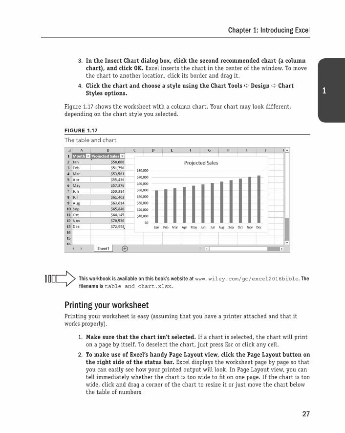
3. In the Insert Chart dialog box, click the second recommended chart (a columnchart), and click OK. Excel inserts the chart in the center of the window. To move the chart to another location, click its border and drag it.

4. Click the chart and choose a style using the Chart Tools ➪ Design ➪ Chart Styles options.

Figure 1.17 shows the worksheet with a column chart. Your chart may look different,depending on the chart style you selected.

FIGURE 1.17

The table and chart.

This workbook is available on this book’s website at www.wiley.com/go/excel2016bible. The

fi lename is table and chart.xlsx.

Printing your worksheetPrinting your worksheet is easy (assuming that you have a printer attached and that itworks properly).

1. Make sure that the chart isn’t selected. If a chart is selected, the chart will print on a page by itself. To deselect the chart, just press Esc or click any cell.

2. To make use of Excel’s handy Page Layout view, click the Page Layout button on the right side of the status bar. Excel displays the worksheet page by page so thatyou can easily see how your printed output will look. In Page Layout view, you can tell immediately whether the chart is too wide to fi t on one page. If the chart is too wide, click and drag a corner of the chart to resize it or just move the chart below the table of numbers.

28


3. When you’re ready to print, choose File ➪ Print. At this point, you can changesome print settings. For example, you can choose to print in landscape rather thanportrait orientation. Make the change, and you see the result in the preview window.

4. When you’re satisfied, click the large Print button in the upper-left corner. Thepage is printed, and you’re returned to your workbook.

Saving your workbookUntil now, everything that you’ve done has occurred in your computer’s memory. If the power should fail, all may be lost — unless Excel’s AutoRecover feature happened to kickin. It’s time to save your work to a fi le on your hard drive.

1. Click the Save button on the Quick Access toolbar. (This button looks like an old-fashioned fl oppy disk, popular in the previous century.) Because the work-book hasn’t been saved yet and still has its default name, Excel responds with a Backstage screen that lets you choose the location for the workbook fi le. The Backstage screen lets you save the fi le to an online location or to your local computer.

2. Click Browse. Excel displays the Save As dialog box.

3. In the File Name field, enter a name (such as Monthly Sales Projection). If you like, you can specify a different location.

4. Click Save or press Enter. Excel saves the workbook as a fi le. The workbook remains open so that you can work with it some more.

By default, Excel saves a backup copy of your work automatically every ten minutes. To adjust the AutoRecover set-

ting (or turn if off), choose File ➪ Options and click the Save tab of the Excel Options dialog box. However, you

should never rely on Excel’s AutoRecover feature. Saving your work frequently is a good idea.

If you’ve followed along, you may have realized that creating this workbook was not dif-fi cult. But, of course, you’ve barely scratched the surface of Excel. The remainder of thisbook covers these tasks (and many, many more) in much gr eater detail.

Documents

Getting Starte Excel COPYRIGHTED MATERIAL · much of this information may se em like review. Even so, it’s likely that you’ll ﬁ nd ... Excel is the world’s most widely used