Embed Size (px)
Citation preview
Getting Rich Too Fast? Voters’ Reactions to Politicians’Wealth Accumulation
Simon Chauchard∗
SIPA, Columbia UniversityMarko Klasnja†
Georgetown University
S.P.Harish‡
College of William & Mary
∗Corresponding author. Email: [email protected].†Address: School of Foreign Service and Government Department ICC 593, Washington
D.C. 20057. Email: [email protected].‡Address: Tyler Hall, 300 James Blair Drive, Williamsburg, VA 23185. Email: sphar-
0
Abstract
Asset declarations requiring politicians to disclose their financial information arebecoming increasingly common across the world. The information contained in thesedisclosures frequently reveals that politicians rapidly accumulate wealth while in office,a fact that may raise suspicion among voters. However, little is known about theways in which such information may impact voter behavior. To address this gap, weutilize original experimental and survey data from India to explore voters’ reactionsto information about wealth and wealth accumulation. Results suggest that votersstrongly disapprove of wealth accumulation in office, and associate it with corruptionand political violence. Further analyses suggest several mechanisms that may partlyexplain why many “wealth accumulators” win elections in India despite these negativereactions. Voters generally lack information about disclosures, and many weigh wealthaccumulation less than some other prominent concerns, such as performance in officeor caste-based appeals.
Keywords: Transparency; Accountability; Corruption; India; Financial Disclosure
Supplementary material for this article is available in the appendix in the online edition.Replication files are available in the JOP Data Archive on Dataverse (http://thedata.harvard.edu/dvn/dv/jop). This study was conducted in compliance with relevant lawsgoverning research involving human participants. The study was approved by the IRB com-mittees at Dartmouth College, Princeton University, and New York University. Support forthis research was provided by Dartmouth College and the Center for the Study of DemocraticPolitics at Princeton University.
Asset declarations requiring politicians to disclose their financial information, such as
income, assets, and liabilities, are becoming increasingly common across the world. While
only 22 countries had such a system in place in 1980, 161 countries had it in 2015. At
present, more than 80 countries make these disclosures public to some extent (Rossi, Pop
and Berger, 2016). As a result, asset disclosures have become the focus of increasing public
interest.1
The data from asset disclosures reveal that in a variety of contexts politicians enjoy
substantial wealth accumulation while in office, often higher than among similar individuals
not in office (Fisman, Schulz and Vig, 2014; Klasnja, 2015; Querubın and Snyder, 2013).
Such evidence may raise suspicions—or at least interest—among voters. This is usually one
of the intended goals of adopting a system of financial disclosures (Djankov et al., 2010;
Rossi et al., 2012). However, currently, there is little evidence on how information about
politicians’ wealth accumulation may impact voters and their evaluations of such politicians.
We begin addressing this gap. Relying on estimates based on official financial disclosures,
and using original experimental and survey data, we explore three interrelated questions:
How do voters generally react to information about wealth and wealth accumulation in
office? To what extent do they associate large wealth accumulation with corruption and
other bad outcomes? How may these evaluations impact electoral behavior, and in turn,
potentially the election of wealth-accumulating politicians?
We examine these questions by drawing on evidence from India. Asset declarations
are part of public affidavits filed as a prerequisite for candidacy for political office. The
disclosures contain candidates’ household-level income tax returns and information about
1Mentions of asset disclosures in the global written corpus (as provided by Google) has
increased more than 14-fold over this period; see Figure A1 in the Supplementary Appendix.
Henceforth, references to sections, tables, and figures with “A” in the title point to the
Supplementary Appendix.
2
assets and liabilities, which also makes it possible to calculate changes in wealth of rerunning
candidates by comparing the information from successive disclosures.2 Such calculations,
done routinely by the press and civil society organizations, point to large increases in wealth
in office among Indian office-holders. For example, the average nominal wealth increase
among Indian state legislators during a five-year legislative term is around 350 percent,
compared to just 17 percent among Indian households over the same time span.3
To understand citizens’ reactions to representatives’ wealth accumulation in such an envi-
ronment, we fielded two surveys to socially diverse samples of citizens in the northern Indian
state of Bihar, where politicians’ wealth accumulation closely resembles national trends (see
Figure A7). The key part of our first survey is a lab-in-the-field conjoint experiment (Hain-
mueller, Hopkins and Yamamoto, 2014), in which our respondents evaluated several fictional
but realistic politician profiles. We randomly varied a number of politician characteristics,
both those commonly examined in the recent literature on Indian politics (Chandra, 2004;
Vaishnav, 2017), such as party affiliation and ethnicity, and for the first time, information
about politicians’ wealth and wealth increase. This design serves our research questions well,
by allowing us to causally identify and compare the weight respondents place on wealth ac-
cumulation relative to other politician attributes, and explore potential interactions between
wealth accumulation and other politician and respondent characteristics likely playing a role
in voter evaluations. The conjoint design also increases the realism of our experiment com-
pared to more traditional survey experiments and lessens concerns over social desirability
bias.
2We describe in more detail the content and the timing of these affidavits in Section 1.1
below.3The estimate for Indian state legislators is based on the data from the Association for
Democratic Reforms, myneta.info; for the households, the source is the India Demographic
and Health Survey, http://ihds.umd.edu/assetscale.html.
3
We complement our conjoint experiment survey with a second survey, the goal of which
was to evaluate citizens’ awareness of asset disclosures, recollection of the information con-
tained in them, and the precision of respondents’ guesses about actual representatives’ wealth
accumulation.
Results from the conjoint experiment indicate that our respondents strongly disapprove
of wealth accumulation in office. They are on average less likely to cast a hypothetical vote
for politician profiles with greater wealth increase, and rate their quality as representatives
significantly lower. Respondents also view greater “wealth accumulators” as more corrupt,
and more prone to violence, an important problem in Bihari and Indian politics (Vaishnav,
2017).
However, these strong negative reactions by our respondents seem at odds with the fact
that many Indian politicians who rapidly accumulate wealth during their tenure manage to
win reelection (see Figure A3). While the election and reelection of wealth accumulators may
in part owe to dynamics we cannot explore in this paper—for example, wealth-accumulating
politicians’ usefulness to parties due to their campaign financing prowess—we utilize our
data to explore several possible mechanisms by which voter behavior may contribute to the
prevalence of large wealth accumulation among politicians in office.
Relying on the data from the second survey, we first find that the majority of our respon-
dents are unaware of the disclosures and their contents, and lack a precise sense of the size of
their actual representatives’ wealth increase. Returning to our conjoint experiment, we also
explore the extent to which the broader structure of voter preferences may prevent negative
reactions to information about politicians’ wealth accumulation from potentially having a
larger impact in actual elections. While our respondents’ disapproval of large wealth increases
by incumbents is overall robust, two results are worth of note. First, respondents weighed
information about a politician’s record in office more heavily than information about wealth
accumulation—even when presented as suspicious. Second, members of the largest caste in
4
the state of Bihar are willing to tolerate very large wealth increases of politicians from a
prominent party focusing mainly on reversing caste inequalities rather than on performance
and integrity. These results suggest that voters may not express their distaste for “wealth
accumulators” in elections because they typically remain unaware of their politicians’ assets
and level of wealth accumulation. Also, reactions to information about wealth accumulation,
however negative they might be, may not always be strong enough to prevail over reactions
to politicians’ other characteristics or to performance on other dimensions.
1 How do Voters React to Information About Wealth
Accumulation in Office?
Popular narratives and academic studies in developing democracies indicate that incumbents
often enrich themselves at a rapid pace while in office (Baltrunaite, 2014; Fisman, Schulz
and Vig, 2014; Klasnja, 2015; World Bank; UNODC, 2013).4 Data from India illustrates this
well. For example, in the state of Bihar—where we ran our surveys—a state legislator on
average quadruples their wealth over the span of just one term (which is close to the average
for state legislators across India, as seen in Figure A7). Wealth increases are on average
even higher among politicians in the executive branch and the national legislature (Fisman,
Schulz and Vig, 2014).
How might voters react to information about politicians’ wealth accumulation? It is
plausible that they view large wealth increases in office negatively, especially if changes
in their own wealth are out of line with those of politicians, or if they are not presented
4Existing evidence from established democracies, though limited, suggests smaller levels of
accumulation than in developing countries (Amore, Bennedsen and Nielsen, 2015; Kotakorpi,
Poutvaara and Tervio, 2015). Eggers and Hainmueller (2009), however, show that post-
tenure wealth increase in the UK can be quite large.
5
with reasonable explanations for such politicians’ enrichment (Di Tella and Weinschelbaum,
2008). While the literature has not so far generated specific expectations regarding voters’
views on politicians’ wealth accumulation, studies have shown that voters often—though not
always—disapprove of corruption or criminality (e.g. Banerjee et al., 2014; Ferraz and Finan,
2008; Klasnja, Tucker and Deegan-Krause, 2016). Moreover, recent studies indicate that the
adoption of financial disclosures can improve the quality of the candidate pool, suggesting
that corrupt politicians may expect voters to punish them for information on malfeasance
potentially revealed through the disclosures (Fisman, Schulz and Vig, 2016; Szakonyi, 2017).
It is nonetheless also possible that voters may sometimes either value politicians’ wealth
accumulation or be indifferent to it. Voters may view large wealth increase as a signal
of skill, drive, or some other desirable characteristic. For example, in the aftermath of
the Mani pulite (“Clean Hands”) investigations that exposed systemic corruption in Italian
politics, Silvio Berlusconi’s supporters touted his $13.5 million in net annual earnings as a
signal of uomo forte—a strong man who would employ his business acumen for effective and
incorruptible leadership.5 In the Indian context, certain groups of voters, especially when
evaluating certain types of politicians, have been argued to value politicians’ willingness to
break the law (Vaishnav, 2017). Moreover, prominent models of voting behavior emphasize
ethnicity and party labels as central criteria in Indian voters’ choices, suggesting that they
may be largely indifferent to other politician features (Chandra, 2004).
Given these contrasting expectations, we first seek to understand how voters generally
react to information about politicians’ wealth increase, and what kind of inferences about
politicians they may make based on this type of information.
5See: http://www.nytimes.com/2013/02/27/opinion/global/why-italians-vote-
for-berlusconi.html.
6

1.1 Research Design: The Conjoint Experiment
For this purpose, we asked a socially diverse sample of citizens in the northern Indian state
of Bihar to take part in a conjoint experiment in which they evaluated candidates on several
dimensions, including wealth and wealth accumulation (N = 1, 020).
Setting
Bihar is a good fit for both practical and substantive reasons. Practically, state elections took
place (in the fall of 2015) six months after the time we fielded our surveys (in the spring of
2015), providing us with a relevant setting to measure likely voter evaluations of prospective
candidates. Substantively, Bihar is a state with relatively high levels of corruption (Witsoe,
2013; Vaishnav, 2017), and the average rate of wealth accumulation among state legislators
is comparable to that in the rest of the country (Figure A7).
Our study took place in a lab-in-the-field setting in the Madhepura district, in the north-
eastern part of the state. We chose to focus on only one district and bring respondents to
a lab to avoid misreporting and unrecorded errors arising from implementing a complex,
randomized survey experiment in an environment with high illiteracy and low levels of pri-
vacy (Chauchard, 2013). A single lab-in-the-field location allowed us to better monitor the
work of our enumerators, ensure that interviews were both private and confidential, and to
carefully tailor and control the presentation of survey information.
Because we wanted rural respondents to constitute the majority of the sample, in order to
reflect the population of Bihar (which is over 85 percent rural), we targeted districts whose
capital city counted fewer than 50,000 inhabitants. Madhepura was randomly selected among
districts fitting this criterion. We show in Figure A8 that Madhepura resembles North India
7
on a number of relevant dimensions.6
Our sampling procedure, described in detail in Section A5, attracted a diverse sample
of respondents to our lab location. Table A3 shows that our sample is broadly similar on
a number of demographic characteristics to the populations of Bihar and North India. As
a result, we believe our inferences are broadly informative about the preferences of North
Indian voters.
Upon arriving to the lab, participants first responded to a short survey eliciting their de-
mographic and socio-economic information (questionnaires used in this study can be found in
Section A13 of the Appendix). The respondents were then presented with three experimental
vignettes, each featuring a photograph and a summary of the randomly assigned attributes
of the politician (see the example in Figure A9), and subsequently asked to evaluate the
politician on several dimensions, as described below. Following the experiment, participants
answered several additional questions measuring their knowledge about and involvement in
politics.
Summary of Manipulations
The vignettes showed a profile of a fictitious politician that enumerators described as a
“current state legislator and likely candidate in the upcoming state elections.”7 Using ficti-
tious candidates allowed us to randomly assign politician attributes, which would have been
impossible and unethical with real politicians.
6Madhepura, however, is more rural and has a higher share of illiterate citizens than the
majority of districts in North India (see Figure A8).7All respondents were debriefed at the end of the post-treatment survey and told that the
profiles were fictitious. Our enumerators reported that less than four percent of the respon-
dents may not have perceived the politicians as real. Our results are robust to excluding
these observations.
8
Each vignette featured eight attributes of the politician (see Figure A9). To randomly
manipulate this large number of attributes, we rely on the conjoint design formalized by
Hainmueller, Hopkins and Yamamoto (2014). Conjoint vignettes allow for richer profiles
and more realistic experiments than more traditional survey experimental designs.8 This
richness is also useful for limiting social desirability: if each profile contains several pieces
of information, it becomes difficult for respondents to guess the subject of researchers’ in-
vestigations, and less likely that they will refrain from endorsing potentially controversial
attributes.
Our key attributes of interest concern the politician’s wealth increase between 2010 and
2015 (i.e. during the 2010-2015 session of the Bihar state assembly), and their wealth at
the beginning of this period. These treatments were modeled on real-life disclosures. The
financial information is one of the components of an affidavit filed by each electoral candidate
with local representatives of the Election Commission of India (ECI), two to three weeks
prior to election day. The ECI makes the affidavits public shortly thereafter. The financial
information consists of income from household-level tax returns and the stock of assets
(movable and immovable) and liabilities at the end of the previous calendar year. In addition
to this information, the affidavits contain contact and basic family information, candidate’s
age, profession, education, criminal record, and party affiliation. Sample pages from a real
affidavit are shown in Section A14.
The affidavits do not provide information on wealth increase. However, since they con-
tain monetary totals, it is not difficult to calculate wealth changes for candidates running in
8Our choice of attributes was guided by how real-world candidates are usually presented.
We do not find evidence of “survey satisficing,” i.e. overwhelming respondents with too
much information (Bansak et al., 2018), as our enumerators reported that 90 percent of
respondents were focused and gave attentive responses. Further, our key attributes do not
have stronger effects when listed first or last (see Figure A10).
9
successive elections.9 Indeed, many press and civil society organizations, such as the Asso-
ciation for Democratic Reforms, compile such data, present appealing visualizations in both
English and vernacular languages, and stress cases of particularly large wealth accumula-
tion.10 Examples of media and civil society reports are shown in Figures A4-A6.
For the 2010 wealth treatment, the possible values in the vignette were: 5 lakhs, 8 lakhs,
45 lakhs, 85 lakhs, 2 crores and 4 crores rupees (a lakh is 100,000 rupees; a crore is 10
million rupees). These values correspond roughly to the 5th, 10th, 25th, 50th, 75th, 90th,
and 95th percentile of the distribution of 2010 wealth reported in affidavits of incumbent
representatives (MLAs) in Bihar. To simplify the presentation of results, we group these
treatments into three categories of 2010 wealth: below median, median–75th percentile,
above 75th percentile.11
We also use seven values for the wealth increase treatment: no increase, 20% increase,
increase of two, three, five, ten, and thirty times.12 These values also roughly correspond
9The rerunning rate among incumbent state legislators is 76 percent in India, 71 percent
in Bihar (over the last two cycles).10The frequency of mentions of asset disclosures in the English-language Indian press has
increased close to 7-fold since their introduction in 2004, particularly around elections. See
Figure A2.11The disclosures are self-reports. It is probably safe to assume that candidates do not
overestimate their wealth in the affidavits, but we cannot exclude the possibility that they
under-report it, despite the prescribed monetary fees and a potential prison sentence of up
to six months for false disclosure (Article 125A of the Representation of the People Act). We
believe, however, that this is of limited concern for our analyses: citizens have access only
to the self-reported information; moreover, our results suggest that voters would probably
react even more negatively to large wealth accumulation if there were no under-reporting.12We presented the 20% condition as “slight increase,” because our pre-testing and past
experience of doing surveys in India and Bihar revealed that many of our respondents find
10
to the 5th, 10th, 25th, 50th, 75th, 90th, and 95th percentile in the distribution of the
observed wealth increase among rerunning MLAs in Bihar for 2005-2010. Ten-fold and larger
wealth increases are by no means unheard of—eleven state legislators in Bihar had wealth
accumulation between 2010 and 2015 in excess of 900 percent. For simplicity, we present the
results by also grouping these treatments into three categories: no increase, below-median
increase, and above-median increase.13
Finally, when a profile featured wealth increase (i.e. not a “no increase” condition), we
also randomly varied its perceived legality, by adding text on whether the press had or had
not reported suspicions of illegality related to this wealth accumulation.
Beyond these wealth-related manipulations, the experiment randomized five other candi-
date attributes, either also reported in the affidavits or commonly presented in the campaign
and media profiles of Indian politicians: party affiliation, ethnicity, performance in office (i.e.
record), social background, and whether they faced criminal charges. These factors are widely
studied in the literature on candidate evaluations in India and more broadly (Chandra, 2004;
Prakash, Rockmore and Uppal, 2015; Vaishnav, 2017; Chauchard, Forthcoming).
Regarding the ethnicity of the candidate, because of the large number of subcastes in
Bihar (more than fifty in our sample alone), we ensured that one of the three politicians
rated by each respondent was from the subcaste of the respondent, which we obtained in
the pre-treatment demographic survey. For the remaining two profiles, we randomly drew
from a list of the eleven largest subcastes in Madhepura. The party of the candidate was
a random draw among the RJD, JD(U), BJP and the Congress (INC), parties that get the
lion’s share of the vote in Bihar. Regarding record in office, politicians were described as
having been “[very active/not very active] in terms of development and infrastructure,” and
having done “[a lot/very little] for his constituency.” For the social background treatment,
percent changes challenging to interpret.13Our main results are substantively the same if we use all seven values (Figure A15).
11
we varied whether the politician originally hailed from a “poor,” “middle income” or “rich”
family (before they entered politics). Finally, for the criminality treatment, the politician
was described as either “not charged in any criminal cases” or “charged in several criminal
cases.”14
The experimental vignettes were the product of three sets of randomizations—of the
values of each attribute, the order of attributes in the vignette, and the order in which
the vignettes were presented to the respondents. Section A7 gives more details on the
randomization procedure. Section A9 shows through a series of diagnostic tests that our
randomizations were successfully implemented (see Tables A5 and A6, and Figure A10).
Outcome Variables
Following the presentation of each vignette, respondent were asked five outcome questions
(reproduced in full in Section A13): (1) whether they would consider voting for the politician
(yes/no); (2) how good a job the politician would do in addressing constituents’ problems
(1–5 scale); (3) how helpful the politician would be for the respondent personally (1–5 scale);
(4) how likely it is that the politician was corrupt (1–5 scale); and (5) how likely it is that
the politician would engage in violent activities (1–5 scale).
In the main text, we focus primarily on the respondents’ hypothetical votes, and report
the results for the other outcomes in the Supplementary Appendix. While the preferences
elicited through the voting question cannot be equated with actual voting decisions, they
provide us with insights about the kinds of politicians the voters generally value and prefer.
Figures A17 and A18 show that our results are very similar when using the questions on the
politician’s quality as a representative (items 2 and 3 above).
14The remaining two treatments—the face of the politician, and the district in which the
politician planned to run—are not of theoretical interest, but Table A10 shows that they
generally have null effects and do not interact with the wealth accumulation treatments.
12
1.2 Voters’ Strongly Negative Reactions to Wealth Accumulation
We start by examining the treatment effects of information about wealth accumulation and
other attributes on respondents’ vote intentions. Following Hainmueller, Hopkins and Ya-
mamoto (2014), we estimate the average marginal component effects (AMCE) for each of our
treatment conditions, commonly reported in studies employing the conjoint design (see also
Egami and Imai, 2017). The AMCE is the effect of a change in the value of an attribute,
averaged over the joint distribution of all other attributes. For example, the AMCE for
the above-median wealth increase measures the ceteris paribus change in the respondent’s
probability of voting for the candidate when the respondent is shown a candidate profile
with above-median wealth increase compared to a profile with another value of wealth ac-
cumulation. The ceteris paribus effect is obtained by calculating this wealth increase effect
for every combination of the other attributes, and then taking the weighted average, where
the weights are based on the frequency with which each combination of the other attributes
appears in our sample.15 For two attributes—party and ethnicity—we examine the effect of
co-partisanship and co-ethnicity between the respondent and the candidate profile, rather
than the effects of a candidate’s party and ethnicity per se, which are not of theoretical
interest.16
We specify a base category for each candidate attribute, to which we compare the effects
of other attribute values. Our base politician profile shares the partisan affiliation and
ethnicity of the respondent, has a good record in office, no criminal charges, comes from a
poor background, has below-median initial wealth, and did not increase his wealth during
the current term in office. In the rest of this article, our effects for any attribute are always
15Since the information about the legality of wealth accumulation is conditional on wealth
increase, the legality AMCE is not defined for profiles featuring no wealth increase.16For the ethnicity treatment, the procedure to calculate the AMCE is somewhat different
than for the other AMCEs, and it is described in detail in Section A8.
13
relative to these reference categories, unless stated otherwise.
Figure 1 shows the results; the point estimate and p-value (in brackets) for each treat-
ment effect are shown on the right side of the plot.17 As can be seen from the estimates at
the bottom of the figure, respondents strongly penalized candidates who were presented as
having accumulated greater wealth in office. The treatment effects of the “below median”
and “above median” wealth increase (relative to “no increase”) are both negative and highly
statistically significant. The magnitude of these effects is not trivial: the penalty for above-
median wealth increase is about 26 percentage points, or about 40 percent of the average
probability of voting for any profile. Although participants penalized all wealth accumula-
tion, the magnitude of wealth accumulation clearly mattered.18 The effect for the below-
median wealth increase treatment is about 35 percent smaller than for above-median wealth
increase, and the difference between the two effects is statistically significant at p = .001.
Intuitively, suspicions of illegal wealth increase on average accentuate the negative effect
of wealth increase on the vote intention (the bottom-most AMCE in Figure 1). However, as
shown in Figure A19, even when respondents are explicitly told that the press reports no
suspicions of illegality, high wealth increase (ten-fold or thirty-fold) results in a statistically
significant lower probability of vote (at p < .032 or lower).19
17This and all subsequent graphs show the 95 percent confidence intervals. The AM-
CEs for photographs and districts are excluded. The results for these treatments are
shown in Table A10. The estimated model is: Pr(Vote) = β0 +∑
j β1jWealth increasej +
β2Legality +∑
j β3jWealth increasej × Legality +∑
k
∑l βklOther treatmentskl + ε, where
Other treatmentskl contains k = 8 treatments, with l conditions for each treatment (shown
in Table A4). The errors are clustered by respondent. The results are robust to the addition
of respondent fixed effects and vignette order fixed effects.18Figure A15 disaggregates the results to include all seven values of wealth increase. The
results are substantively the same.19Because both our legality treatment conditions mention the press, the size and signif-
14
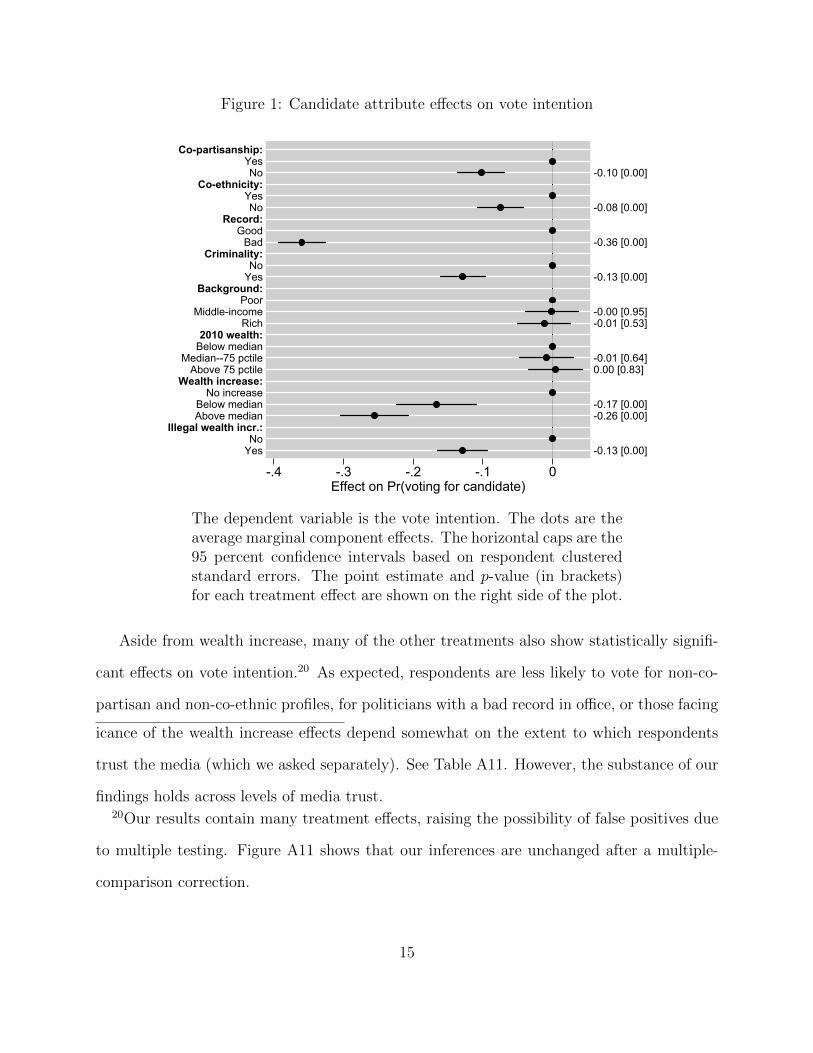
Figure 1: Candidate attribute effects on vote intention
-0.10 [0.00] -0.08 [0.00] -0.36 [0.00] -0.13 [0.00] -0.00 [0.95]-0.01 [0.53] -0.01 [0.64]0.00 [0.83] -0.17 [0.00]-0.26 [0.00] -0.13 [0.00]
Co-partisanship:YesNo
Co-ethnicity:YesNo
Record:Good
BadCriminality:
NoYes
Background:Poor
Middle-incomeRich
2010 wealth:Below median
Median--75 pctileAbove 75 pctile
Wealth increase:No increase
Below medianAbove median
Illegal wealth incr.:No
Yes
-.4 -.3 -.2 -.1 0Effect on Pr(voting for candidate)
The dependent variable is the vote intention. The dots are theaverage marginal component effects. The horizontal caps are the95 percent confidence intervals based on respondent clusteredstandard errors. The point estimate and p-value (in brackets)for each treatment effect are shown on the right side of the plot.
Aside from wealth increase, many of the other treatments also show statistically signifi-
cant effects on vote intention.20 As expected, respondents are less likely to vote for non-co-
partisan and non-co-ethnic profiles, for politicians with a bad record in office, or those facing
icance of the wealth increase effects depend somewhat on the extent to which respondents
trust the media (which we asked separately). See Table A11. However, the substance of our
findings holds across levels of media trust.20Our results contain many treatment effects, raising the possibility of false positives due
to multiple testing. Figure A11 shows that our inferences are unchanged after a multiple-
comparison correction.
15
criminal charges. Note, however, that the effects of information on wealth accumulation
are larger than the effect of most of the other characteristics. The above-median wealth
increase AMCE is statistically significantly larger than AMCEs for ethnicity, partisanship
and criminality at p < .001. The below-median wealth increase is larger than the ethnicity
and partisanship AMCEs at p < .01 and p < .07, respectively.
Responses to the corruption and violence questions indicate that respondents associate
greater wealth accumulation with “bad” outcomes. Greater wealth increase significantly
increased respondents’ perception of a candidate being both more corrupt and more violent
(see Figure A16). Information about wealth information contributes more than any other
attribute to voters’ perceptions about corruption, and is on a par with criminality in terms
of their perceptions of violence.
These negative reactions to politicians’ wealth accumulation are unlikely to be due to
respondents’ anti-rich bias, since we also presented information candidates’ initial level of
wealth and family background. The AMCEs for these treatments are noticeably smaller
than the wealth increase AMCEs, and generally statistically indistinguishable from zero.21
Moreover, because wealth accumulation is one of many manipulated attributes in our design,
and because these effects are large, we deem it unlikely that they owe primarily to a survey
effect or to social desirability bias. The wealth accumulation treatment was one among
ten other treatments, and was not in any way emphasized by the interviewers.22 Besides,
we have no a priori reason to believe that wealth accumulation would be a more sensitive
treatment than ethnicity or criminality. Accordingly, we interpret these responses as strong
21These results also indicate that respondents do not disadvantage poor or working-class
candidates, consistent with recent comparative work (Carnes and Lupu, 2016).22One way to gauge the potential size of the desirability effect is to examine whether
respondents reacted more strongly when the information about wealth accumulation was
(randomly) presented first. We do not find such evidence (see Figure A10).
16
evidence that Bihar voters disapprove of wealth accumulation in office—when shown such
information.
2 Why May Voters’ Negative Evaluations Have Lim-
ited Electoral Consequences?
These findings, while strong, seem at odds with the observation that many representatives
in Bihar and India rapidly accumulate wealth during their tenure and still manage to win
reelection.23 If voters’ reactions to information about wealth accumulation are so negative,
why do we see so many “wealth accumulators” in office? Certainly, the reasons may be
largely unrelated to voter behavior; for example, parties may prefer wealth accumulators for
their greater ability to contribute to party financing, or because they may be more effective
decision-makers. Our data cannot speak to these explanations. Nonetheless, we can examine
several, non-exhaustive mechanisms through which voters may contribute to the prevalence
of high wealth accumulation in office.
To explore these mechanisms, we draw from two related literatures. The first one fo-
cuses on the role of information about politician performance in voter behavior, while the
second examines the preference-related reasons why corrupt or otherwise apparently “bad”
politicians may maintain public support. Based on these literatures, we evaluate two types
of hypotheses: information-related and preference-related.
According to the information hypothesis, voters may in principle disapprove of prob-
lematic candidates, but fail to sanction them simply because they do not possess enough
information about them, whether due to lack of access or lack of attentiveness (e.g. Chong
et al., 2015; de Figueiredo, Hidalgo and Kasahara, 2011; Ferraz and Finan, 2008; Klasnja,
23Figure A3 shows that rerunning state legislators with greater wealth increase on average
exhibit higher reelection rates than those with lower wealth accumulation.
17
2017; Reinikka and Svensson, 2011; Weitz-Shapiro and Winters, 2013). In our case, even
if voters react negatively to information based on asset disclosures when presented with it,
they may otherwise be unaware of the disclosures and the extent of wealth accumulation
among politicians. That they are uninformed before we present them with this information
is however not a foregone conclusion, as citizens may still have a sense of their incumbents’
ability to accumulate wealth even in the absence of precise information, either through direct
observation, or because they have heard about it from others.24
Preferences-based hypotheses, on the other hand, suggest that better information dis-
semination, even if needed, may not suffice. Assuming that voters take several factors into
consideration when evaluating candidates, one possibility is that they may disapprove of
wealth accumulation but put less weight on it relative to some other factor. Drawing on
experimental evidence in the northern Indian state of Uttar Pradesh, Chauchard (2017)
illustrates this logic: voters strongly penalized criminal candidates overall, yet they also
placed lower weight on criminality than ethnicity, thus often favoring criminals from their
own caste compared to “clean” candidates from some particularly disliked groups. This is a
possibility even in the absence of any interaction between the effect of wealth accumulation
and some other factor.
Second, not every wealth accumulator may be equal in voters’ eyes. That is, there
may be explicit interactions between wealth accumulation and other politician (or voter)
attributes, so that (some) voters may be more willing to forgive large wealth accumulation
by certain kinds of politicians. Scholars have shown that voters’ reactions to corruption
24Some politicians acquire wealth during their tenure in an ostentatious manner. In North
India, Mayawati, the former chief minister of the state of Uttar Pradesh, is a case in point
(see Figure A4). When a politician engages in conspicuous consumption—such as buying
real estate and luxury goods—voters may not require estimates drawn from asset disclosures
to conclude that their representative is increasing their wealth.
18
more broadly can be mitigated by politicians’ ethnicity (Banerjee and Pande, 2011), party
affiliation (Anduiza, Gallego and Munoz, 2013; Rundquist, Strom and Peters, 1977), or
class background (Witsoe, 2011). Similarly, voters may excuse corruption by politicians who
otherwise deliver good performance or side benefits to the constituents (Barbera, Fernandez-
Vazquez and Rivero, 2016; Klasnja and Tucker, 2013; Zechmeister and Zizumbo-Colunga,
2013).
We examine each of these arguments in turn.
2.1 How Aware are Voters of Wealth Accumulation?
Despite the public availability of affidavits and the efforts by the press and civil society
organizations to publicize them, little is known about how much voters may know or surmise
about these disclosures or about politicians’ ability to accumulate wealth in office in India.
For this purpose, we fielded a separate survey examining voter awareness of disclosures
and information therein, as well as their perceptions about actual representatives’ wealth
accumulation. The survey was fielded in June 2015 (less than two months after the end of our
conjoint experiment, and four months before the election in Bihar), on a different sample of
Madhepura citizens from that in the first survey (N = 323). The two samples were nonethe-
less drawn from the same district population and are similar on a range of demographic
and socio-economic variables (see Table A2).25 Because the 2015 disclosures were not yet
submitted at the time of the survey, our survey probed our respondents’ awareness of the
disclosures generally, asked about recollections of information from the 2010 disclosures, and
solicited their best guesses about representatives’ wealth increase between 2010 and 2015.
25We did not ask respondents in our first experimental survey about their knowledge of
the disclosures and wealth increase among actual politicians in order not to risk priming
the purpose of the experiment or contaminating the post-treatment answers. The questions
appearing only in the second survey are reproduced in Section A13.4.
19
Overall, the results indicate that our respondents are relatively poorly informed about
the disclosures and the information therein, and do not anticipate with precision their rep-
resentatives’ wealth accumulation.
Roughly half (48%) of our respondents said that they have not heard of these disclosures
before the survey, and two-thirds reported not knowing that these disclosures are public.
In other words, only a third of the sample knew about the disclosures and that they were
accessible.26
If such a minority self-reports being aware of disclosures, it is unlikely that many voters
are very familiar with their contents. Indeed, Figure A12 shows that less than a third of our
respondents were able to correctly guess (or recall) their own MLA’s wealth, as reported in
their most recent affidavit (from 2010). Moreover, even those who are aware of disclosures
were no more likely to furnish correct responses (see Table A7).
It is possibly unrealistic to expect voters to recall particular financial information about
their representatives (from a long time ago, too). As mentioned above, voters may nonethe-
less have a sense of their MLA’s wealth increase even in the absence of detailed knowledge
of the disclosures and their contents. To gauge this possibility, we asked our respondents to
guess what their MLA’s wealth accumulation between 2010 and 2015 may be, even though
such information was not yet calculable because the 2015 affidavits were not yet available.
To anchor the respondents’ answers and decrease measurement error, we offered the same
categories as in our conjoint experiment (no increase, slight increase of 20%, increase of two,
three, five, ten, or thirty times).27
26Nineteen respondents, or about 6%, reported that they knew the disclosures were pub-
lic, yet that they did not hear about the disclosures before. We treat those responses as
unknowledgeable on both questions.27We first asked whether respondents’ thought their MLA’s wealth increased since 2010,
and conditional on a “yes” response, offered the other categories.
20
Our respondents came from one of two constituencies in the Madhepura district, rep-
resented by Chandra Shekhar (the constituency of Madhepura), or Ramesh Rishidev (the
constituency of Singheshwar). The true, post-hoc, observed wealth increase was roughly a
doubling of wealth for Shekhar, and a five-fold increase for Rishidev. Figure 2 plots for each
MLA the proportion of respondents by category (in bars, gray being the correct guess), and
the difference in the predicted probability of each category response from what would be the
correct guess, with the associated 95% confidence intervals (in caps).28
While our respondents are clearly less likely to make extreme guesses (e.g., 10-fold or
30-fold), they are as likely to anticipate a level of wealth increase multiple times lower or
higher than the actual, post-hoc observed, rate (and once again, less than a third made what
was the correct guess). Further, best guesses by the constituents of Rishidev, whose rate of
wealth increase is considerably higher, are not statistically different from those for Shekhar
(based on the Wilcoxon-Mann-Whitney median rank-sum test). Also, respondents reporting
to be aware of the disclosures were no better at making precise guesses (in fact, they were
systematically worse; see Table A7).29
In sum, whereas it may be too much to expect voters to know all of the information
we asked them about, it is reasonably clear that the majority of our respondents do not
possess much information about the disclosures, or a precise sense of their representatives’
wealth accumulation.30 While our design does not allow us to gauge the extent to which
28The predicted probability differences are based on a multinomial logit model of the re-
spondents’ answers on their demographic and socioeconomic characteristics (age, education,
income, own assets, and whether employed in government).29In addition to the recalls and guesses about their own representatives, we asked our
respondents the same for an average MLA in Bihar. While admittedly more difficult to
answer, the responses are of even lower precision (see Figure A13), and the errors were
strongly correlated with the errors made for own MLAs.30As elections approach, the public nature of affidavits may improve these baseline levels
21
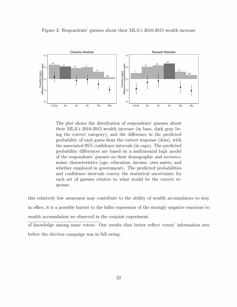
Figure 2: Respondents’ guesses about their MLA’s 2010-2015 wealth increase
.25.21
.19 .2
.12
.027
-.4-.2
0.2
.4
Pro
porti
on (b
ars)
,di
ffere
nce
in p
roba
bilit
ies
(cap
s)
0-0.2x 2x 3x 5x 10x 30x
Chandra Shekhar
.1
.21.23
.27
.12
.067
-.4-.2
0.2
.4
Pro
porti
on (b
ars)
,di
ffere
nce
in p
roba
bilit
ies
(cap
s)
0-0.2x 2x 3x 5x 10x 30x
Ramesh Rishidev
The plot shows the distribution of respondents’ guesses abouttheir MLA’s 2010-2015 wealth increase (in bars, dark gray be-ing the correct category), and the difference in the predictedprobability of each guess from the correct response (dots), withthe associated 95% confidence intervals (in caps). The predictedprobability differences are based on a multinomial logit modelof the respondents’ guesses on their demographic and socioeco-nomic characteristics (age, education, income, own assets, andwhether employed in government). The predicted probabilitiesand confidence intervals convey the statistical uncertainty foreach set of guesses relative to what would be the correct re-sponse.
this relatively low awareness may contribute to the ability of wealth accumulators to stay
in office, it is a possible barrier to the fuller expression of the strongly negative reactions to
wealth accumulation we observed in the conjoint experiment.
of knowledge among some voters. Our results thus better reflect voters’ information sets
before the election campaign was in full swing.
22
2.2 Do Voters Always Disapprove of Wealth Accumulation?
Another possible limit to voters’ negative reactions to politicians’ wealth accumulation may
stem from the particular structure of their preferences. A first possibility is that voters place
less weight on politicians’ wealth increase than on some other factor. If this is the case,
candidates whom voters know to be rapidly accumulating wealth may be preferred due to
some other, more highly valued, characteristic.
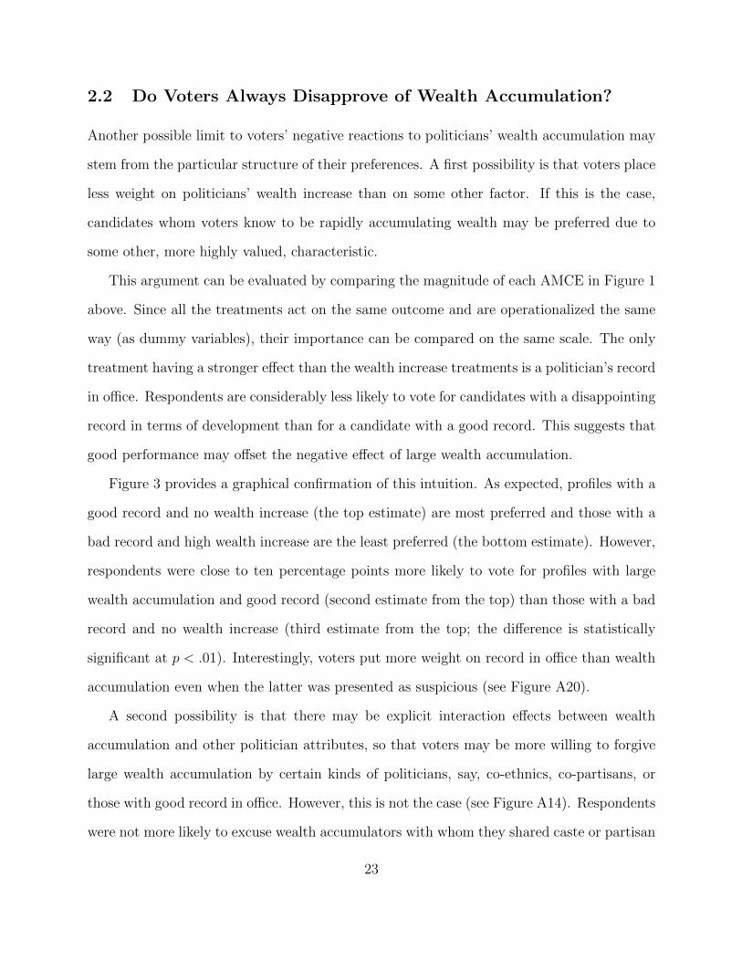
This argument can be evaluated by comparing the magnitude of each AMCE in Figure 1
above. Since all the treatments act on the same outcome and are operationalized the same
way (as dummy variables), their importance can be compared on the same scale. The only
treatment having a stronger effect than the wealth increase treatments is a politician’s record
in office. Respondents are considerably less likely to vote for candidates with a disappointing
record in terms of development than for a candidate with a good record. This suggests that
good performance may offset the negative effect of large wealth accumulation.
Figure 3 provides a graphical confirmation of this intuition. As expected, profiles with a
good record and no wealth increase (the top estimate) are most preferred and those with a
bad record and high wealth increase are the least preferred (the bottom estimate). However,
respondents were close to ten percentage points more likely to vote for profiles with large
wealth accumulation and good record (second estimate from the top) than those with a bad
record and no wealth increase (third estimate from the top; the difference is statistically
significant at p < .01). Interestingly, voters put more weight on record in office than wealth
accumulation even when the latter was presented as suspicious (see Figure A20).
A second possibility is that there may be explicit interaction effects between wealth
accumulation and other politician attributes, so that voters may be more willing to forgive
large wealth accumulation by certain kinds of politicians, say, co-ethnics, co-partisans, or
those with good record in office. However, this is not the case (see Figure A14). Respondents
were not more likely to excuse wealth accumulators with whom they shared caste or partisan
23
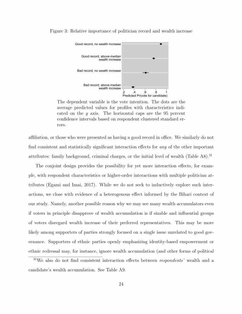
Figure 3: Relative importance of politician record and wealth increase
Good record, no wealth increase
Good record, above-medianwealth increase
Bad record, no wealth increase
Bad record, above-medianwealth increase
.2 .4 .6 .8 1Predicted Pr(vote for candidate)
The dependent variable is the vote intention. The dots are theaverage predicted values for profiles with characteristics indi-cated on the y axis. The horizontal caps are the 95 percentconfidence intervals based on respondent clustered standard er-rors.
affiliation, or those who were presented as having a good record in office. We similarly do not
find consistent and statistically significant interaction effects for any of the other important
attributes: family background, criminal charges, or the initial level of wealth (Table A8).31
The conjoint design provides the possibility for yet more interaction effects, for exam-
ple, with respondent characteristics or higher-order interactions with multiple politician at-
tributes (Egami and Imai, 2017). While we do not seek to inductively explore such inter-
actions, we close with evidence of a heterogenous effect informed by the Bihari context of
our study. Namely, another possible reason why we may see many wealth accumulators even
if voters in principle disapprove of wealth accumulation is if sizable and influential groups
of voters disregard wealth increase of their preferred representatives. This may be more
likely among supporters of parties strongly focused on a single issue unrelated to good gov-
ernance. Supporters of ethnic parties openly emphasizing identity-based empowerment or
ethnic redressal may, for instance, ignore wealth accumulation (and other forms of political
31We also do not find consistent interaction effects between respondents’ wealth and a
candidate’s wealth accumulation. See Table A9.
24
malfeasance).
In the context of Bihar, one such party clearly exists: the Rashtriya Janata Dal party, or
RJD (Witsoe, 2013). Headed by Lalu Prasad Yadav, the RJD has since the 1980s aggressively
promoted the politics of caste empowerment for Yadavs, the most numerous caste in Bihar
(comprising more than 40% of our sample). The party has held executive power several
times since the 1980’s and is part of the ruling coalition that won the 2015 elections. As
documented by Witsoe (2013), RJD leaders have never made corruption the center of their
appeals, and have even sometimes embraced corruption as a necessary means to achieve
redressal for the lower-caste Yadavs.
It is therefore possible that Yadav voters, the core voters of the RJD, would be more
tolerant than others of wealth accumulation, particularly as they evaluate RJD politicians.
Results in Figure 4 are consistent with this expectation. Yadav respondents do not penalize
wealth accumulation when they are presented with an RJD politician (upper-left panel of
the figure), whereas they are more inclined to penalize wealth accumulation (particularly
large wealth accumulation) of candidates from other parties (lower-left panel).32 On the
other hand, non-Yadav respondents penalize wealth accumulation of both RJD (upper-right
panel) and non-RJD politicians (lower-right panel). While these heterogenous effects may
require further theorizing and empirical tests, they potentially point to an important com-
plementary explanation: leaders and parties focusing mainly on a single issue—in the case of
the RJD, perceived intergroup inequalities—may lead to the creation of political “cultures”
that discount the need to monitor corruption.33
32The difference in the wealth increase effects among Yadav respondents between the RJD
and non-RJD candidates is not statistically significant. However, we are strongly constrained
by sample size when examining these sub-group effects.33Our argument is consistent with models emphasizing the role of a single factor, such as
ethnicity, in voters’ choices (Chandra, 2004). Contrary to these models, however, we suggestthat most parties are not monothematic, only some—perhaps especially ethnic parties—are.
25
Figure 4: Reactions to wealth increase among Yadav and non-Yadav respondents for RJDand non-RJD politician profiles
Below-medianwealth increase
Above-medianwealth increase
-.6 -.4 -.2 0 .2Effect on
Pr(voting for candidate)
Yadavs andRJD candidate
Below-medianwealth increase
Above-medianwealth increase
-.6 -.4 -.2 0 .2Effect on
Pr(voting for candidate)
Non-Yadavs andRJD candidate
Below-medianwealth increase
Above-medianwealth increase
-.6 -.4 -.2 0 .2Effect on
Pr(voting for candidate)
Yadavs andnon-RJD candidate
Below-medianwealth increase
Above-medianwealth increase
-.6 -.4 -.2 0 .2Effect on
Pr(voting for candidate)
Non-Yadavs andnon-RJD candidate
The dependent variable is the vote intention. The dots are theaverage marginal component effects. The horizontal caps are the95 percent confidence intervals based on respondent clusteredstandard errors.
3 Discussion
In sum, our analyses suggest that presenting information about politicians’ wealth accu-
mulation strongly influences voters’ evaluations. This however does not necessarily imply
that voters necessarily penalize “wealth accumulators” at the polls. As we have shown, the
majority of voters are unaware of the disclosures and by and large lack a good sense of their
representatives’ wealth accumulation. Moreover, even when informed, voters’ other consid-
erations can take precedence over concerns about politicians’ wealth increases. While other
mechanisms may exist, these results provide potential explanations reconciling our respon-
dents’ disapproval of wealth accumulation with the documented ability of real-life “wealth
26
accumulators” to win elections (Figure A3).
These findings contribute to several literatures. Recent studies have shown that the
adoption of financial disclosures may help improve the quality and honesty of politicians
running for office (Fisman, Schulz and Vig, 2016; Szakonyi, 2017), arguably because corrupt
wealth accumulators are discouraged from running. This is consistent with our evidence
of voter disapproval of large wealth accumulation. At the same time, many incumbents
accumulate large amounts of wealth even when disclosures are public (Fisman, Schulz and
Vig, 2014; Klasnja, 2015). While there may be many reasons for this puzzle, our study
points to several possible explanations as to why voters may fail to sanction such large
wealth accumulation even if in principle they disapprove of it.
More generally, our results contribute to the growing comparative literature examining
voters’ reactions to corruption and other forms of malfeasance in democratic systems. We
complement the focus of much of the literature on voter evaluations of corrupt politicians
(e.g. Rundquist, Strom and Peters, 1977; Weitz-Shapiro and Winters, 2013) or criminal
candidates (Chauchard, 2017; Vaishnav, 2017) with the focus on the related and salient, but
so far neglected dimension of wealth increase.
Moreover, our findings contribute to the literature on the effects of transparency reforms
on accountability. A number of studies have examined the effect on political accountability of
dissemination efforts through channels such as audits, the media, information campaigns (e.g.
leaflets), and civil society (e.g. Arias et al., 2016; Banerjee et al., 2011; Chong et al., 2015;
Ferraz and Finan, 2008). In addition to focusing on a different, increasingly widespread,
transparency initiative (financial disclosures), our study also contributes nuanced insights
about the potential benefits and limitations of increased transparency.
While not entirely surprising, our results show that voters are largely unfamiliar with the
content of the disclosures. Coupled with our finding that citizens strongly disapprove or large
wealth accumulation, the optimistic takeaway is that better efforts to publicize the infor-
27
mation from the disclosures may strengthen accountability mechanisms. However, our other
results potentially temper this optimism, suggesting that the presumed beneficial effects of
disclosures—and more broadly of information—on accountability may be conditional on a
number of contextual factors. In order for information to reach its full potential and have a
real impact at the polls, voters need to not only be aware of it, but also understand it well.
Important challenges to this in India—as in many developing countries—are high illiteracy
rates and low citizen engagement in politics and civic life. Moreover, even when voters are
informed, politician integrity should feature prominently in their voting decisions. This can
be challenging if voters are reliant on targeted goods, or forced to prioritize demanding basic
public services that would otherwise be lacking. Since institutions, groups and organizations
disseminating information often have little control over these contextual factors, our findings
suggest that it may be difficult to make the voter information initiatives more effective in
the short term.
Beyond its effect on public opinion, we believe future work may fruitfully study other
consequences of rapid enrichment of a political elite. Recent data on wealth distribution
in India suggests that the median Indian state legislator (MLA) comfortably sits among
the top one percent.34 What is more, assuming an average 5-year increase in wealth of
350 percent (the average rate of accumulation across all state legislators in the most recent
affidavit data), the majority of state legislators should move into the top one percent in
terms of wealth after a single term in office. This implies not just that representatives are
increasingly dissimilar from the population, but that they are increasingly homogeneous as
a group. Both of these trends may increase representational inequality and overall levels of
inequality, and for that reason deserve further attention.
34Based on Credit Suisse estimates (https://publications.credit-suisse.com/
tasks/render/file/?fileID=5521F296-D460-2B88-081889DB12817E02, page 147).
28
Acknowledgements: For valuable comments and suggestions we thank Dominik Hangart-
ner, Dan Hopkins, Adrienne LeBas, Kristin Michelitch, Natalija Novta, Irfan Nooruddin,
Grigore Pop-Eleches, Peter van der Windt, Matthew Wright, Teppei Yamamoto, and the
participants at the Princeton Experiments Workshop, the Princeton Workshop on Wealth,
Inequality, and Representation, the Political Economy Seminar at Georgetown University,
the 4th DC Area Comparative Politics Workshop, and the audiences at the Annual Meetings
of the Midwest Political Science Association, and the European Political Science Association.
Colin Sawyer provided excellent research assistance.
References
Amore, Mario Daniele, Morten Bennedsen and Kasper Meisner Nielsen. 2015. “Return to
Political Power in a Low Corruption Environment.” Manuscript.
Anduiza, Eva, Aina Gallego and Jordi Munoz. 2013. “Turning a Blind Eye: Experimental
Evidence of Partisan Bias in Attitudes Towards Corruption.” Comparative Political Studies
46(12):1664–1692.
Arias, Eric, Horacio A. Larreguy, John Marshall and Pablo Querubın. 2016. “Priors Rule:
When do Malfeasance Revelations Help and Hurt Incumbent Parties?” Working Paper.
Baltrunaite, Audinga. 2014. “Value of Political Office: Evidence from Lithuania.”
Manuscript.
Banerjee, Abhijit, Donald P. Green, Jeffery McManus and Rohini Pande. 2014. “Are Poor
Voters Indifferent to Whether Elected Leaders Are Criminal or Corrupt? A Vignette
Experiment in Rural India.” Political Communication 31(3):391–407.
Banerjee, Abhijit, Selvan Kumar, Rohini Pande and Felix Su. 2011. “Do Informed Voters
29
Make Better Choices? Experimental Evidence from Urban India.” Manuscript, Harvard
University.
Banerjee, Abhijit V. and Rohini Pande. 2011. “Parochial Politics: Ethnic Preferences and
Politician Corruption.” Unpublished manuscript.
Bansak, Kirk, Jens Hainmueller, Daniel J. Hopkins and Teppei Yamamoto. 2018. “The Num-
ber of Choice Tasks and Survey Satisficing in Conjoint Experiments.” Political Analysis
26(1):112–119.
Barbera, Pablo, Pablo Fernandez-Vazquez and Pablo Rivero. 2016. “Rooting Out Corrup-
tion or Rooting for Corruption? The Heterogenous Electoral Consequences of Scandals.”
Political Science Research and Methods 4(2):379–397.
Carnes, Nicholas and Noam Lupu. 2016. “Do Voters Dislike Politicians from the Working
Class?” American Political Science Review 110(4):832–844.
Chandra, Kanchan. 2004. Why Ethnic Parties Succeed: Patronage and Ethnic Head Counts
in India. Cambridge, UK: Cambridge University Press.
Chauchard, Simon. 2013. “Using MP3 Players in Surveys The Impact of a Low-Tech Self-
Administration Mode on Reporting of Sensitive Attitudes.” Public Opinion Quarterly
77(1):220–231.
Chauchard, Simon. 2017. “Is Ethnic Politics Responsible for Criminal Politics? A Vignette-
Experiment in North India.” Manuscript, Dartmouth College.
Chauchard, Simon. Forthcoming. “Unpacking Ethnic Preferences: Theory and Micro-Level
Evidence from North India.” Comparative Political Studies .
30
Chong, Alberto, Ana L. De La O, Dean Karlan and Leonard Wantchekon. 2015. “Does Cor-
ruption Information Inspire the Fight or Quash the Hope? A Field Experiment in Mexico
on Voter Turnout, Choice, and Party Identification.” The Journal of Politics 77(1):55–71.
de Figueiredo, Miguel, Daniel Hidalgo and Yuri Kasahara. 2011. “When do Voters Punish
Corrupt Politicians? Experimental Evidence from Brazil.” Working Paper.
Di Tella, Rafael and Federico Weinschelbaum. 2008. “Choosing Agents and Monitoring
Consumption: A Note on Wealth as a Corruption-Controlling Device.” The Economic
Journal 118(532):1552–1571.
Djankov, Simeon, Rafael La Porta, Florencio Lopez-de Silanes and Andrei Shleifer. 2010.
“Disclosure by Politicians.” American Economic Journal: Applied Economics 2(2):179–
209.
Egami, Naoki and Kosuke Imai. 2017. “Causal Interaction in Factorial Experiments: Appli-
cation to Conjoint Analysis.” Manuscript, Princeton University.
Eggers, Andrew C. and Jens Hainmueller. 2009. “MPs for Sale? Returns to Office in Postwar
British Politics.” American Political Science Review 103(4):513–533.
Ferraz, Claudio and Frederico Finan. 2008. “Exposing Corrupt Politicians: The Effects of
Brazil’s Publicly Released Audits on Electoral Outcomes.” Quarterly Journal of Economics
123(2):703–745.
Fisman, Raymond, Florian Schulz and Vikrant Vig. 2014. “Private Returns to Public Office.”
Journal of Political Economy 122(4):806–862.
Fisman, Raymond, Florian Schulz and Vikrant Vig. 2016. “Financial Disclosure and Political
Selection: Evidence from India.” Manuscript.
31
Hainmueller, Jens, Daniel J. Hopkins and Teppei Yamamoto. 2014. “Causal Inference in
Conjoint Analysis: Understanding Multi-Dimensional Choices via Stated Preference Ex-
periments.” Political Analysis 22(1):1–30.
Klasnja, Marko. 2015. “Corruption and the Incumbency Disadvantage: Theory and Evi-
dence.” Journal of Politics 77(4):928–942.
Klasnja, Marko. 2017. “Uninformed Voters and Corrupt Incumbents.” American Politics
Research 45(2):256–279.
Klasnja, Marko and Joshua A. Tucker. 2013. “The Economy, Corruption, and the Vote:
Evidence from Experiments in Sweden and Moldova.” Electoral Studies 32(3):536–543.
Klasnja, Marko, Joshua A. Tucker and Kevin Deegan-Krause. 2016. “Pocketbook vs. So-
ciotropic Corruption Voting.” British Journal of Political Science 46(1):67–94.
Kotakorpi, Kaisa, Panu Poutvaara and Mrko Tervio. 2015. “Returns to Office in National
and Local Politics.” Manuscript.
Prakash, Nishith, Marc Rockmore and Yogesh Uppal. 2015. “Do Criminally Accused Politi-
cians Affect Economic Outcomes? Evidence from India.” Manuscript.
Querubın, Pablo and James M. Jr. Snyder. 2013. “The Control of Politicians in Normal Times
and Times of Crisis: Wealth Accumulation by U.S. Congressmen, 1850-1880.” Quarterly
Journal of Political Science 8:409–450.
Reinikka, Ritva and Jakob Svensson. 2011. “The Power of Information in Public Services:
Evidence from Education in Uganda.” Journal of Public Economics 95(7):956–966.
Rossi, Ivana M., Laura Pop, Francesco Clementucci and Lina Sawaqed. 2012. “Using As-
set Disclosure for Identifying Politically Exposed Persons.” World Bank, Washington
32
DC, https://openknowledge.worldbank.org/handle/10986/26790, License: CC BY
3.0 IGO.
Rossi, Ivana M., Laura Pop and Tammar Berger. 2016. Getting the Full Picture on Public
Officials: A How-to Guide for Effective Financial Disclosure. Washington DC: The World
Bank.
Rundquist, Barry S., Gerald S. Strom and John G. Peters. 1977. “Corrupt Politicians and
Their Electoral Support: Some Experimental Observations.” American Political Science
Review 71(3):954–963.
Szakonyi, David. 2017. “Anti-Corruption Campaigns and Political Selection: Evidence from
Russia.” SSRN Working Paper.
Vaishnav, Milan. 2017. When Crime Pays: Money and Muscle in Indian Politics. New
Haven: Yale University Press.
Weitz-Shapiro, Rebecca and Matthew S. Winters. 2013. “Lacking Information or Condon-
ing Corruption? Voter Attitudes Toward Corruption in Brazil.” Comparative Politics
45(4):418–436.
Witsoe, Jeffrey. 2011. “Corruption as Power: Caste and the Political Imagination of the
Postcolonial State.” American Ethnologist 38(1):73–85.
Witsoe, Jeffrey. 2013. Democracy against Development: Lower-Caste Politics and Political
Modernity in Postcolonial India. Chicago, IL: University of Chicago Press.
World Bank; UNODC. 2013. “Income and Asset Disclosure: Case Study Illustrations.” Direc-
tions in Development Finance. Washington, DC: World Bank, https://openknowledge.
worldbank.org/handle/10986/13835, License: CC BY 3.0 IGO.
33
Zechmeister, Elizabeth J. and Daniel Zizumbo-Colunga. 2013. “The Varying Political Toll of
Concerns about Corruption in Good Versus Bad Economic Times.” Comparative Political
Studies 46(10):1190–1218.
Simon Chauchard is a lecturer-in-discipline at the School of International and Public
Affairs (SIPA) at Columbia University, New York City, NY 10027. Marko Klasnja is an
assistant professor at Georgetown University, Washington, DC 20057. S.P. Harish is an
assistant professor at the College of William and Mary, Williamsburg, VA 23185.
34