Geophysical Journal International - ESC Publicationseprints.esc.cam.ac.uk/3601/7/Geophys. J. Int.-2016-Pugh-275-91.pdfGeophysical Journal International Geophys. J. Int. (2016) 206,

Geophysical Journal InternationalGeophys. J. Int. (2016) 206, 275–291 doi: 10.1093/gji/ggw146Advance Access publication 2016 April 20GJI Seismology

Automatic Bayesian polarity determination

D.J. Pugh,1,2,∗ R.S. White1 and P.A.F. Christie2

1Bullard Laboratories, Department of Earth Sciences, University of Cambridge, Cambridge CB3 0EZ, United Kingdom. E-mail: [email protected] Gould Research, High Cross, Cambridge, United Kingdom

Accepted 2016 April 11. Received 2016 April 9; in original form 2015 September 24

S U M M A R YThe polarity of the first motion of a seismic signal from an earthquake is an important constraintin earthquake source inversion. Microseismic events often have low signal-to-noise ratios,which may lead to difficulties estimating the correct first-motion polarities of the arrivals.This paper describes a probabilistic approach to polarity picking that can be both automatedand combined with manual picking. This approach includes a quantitative estimate of theuncertainty of the polarity, improving calculation of the polarity probability density functionfor source inversion. It is sufficiently fast to be incorporated into an automatic processingworkflow. When used in source inversion, the results are consistent with those from manualobservations. In some cases, they produce a clearer constraint on the range of high-probabilitysource mechanisms, and are better constrained than source mechanisms determined using auniform probability of an incorrect polarity pick.

Key words: Numerical solutions; Probability distributions; Earthquake ground motions;Earthquake source observations; Computational seismology; Statistical seismology.

1 I N T RO D U C T I O N

First-motion-based source inversion of earthquakes can be used toconstrain nodal planes and to help estimate the source parameters.The use of first-motion polarities was proposed by Nakano (1923)and first implemented by Byerly (1926). These first-motion polar-ities of the phase arrivals provide an important constraint on thefocal mechanism.

There are several source inversion approaches that utilize first-motion polarities to determine the source type, such as FPFIT(Reasenberg & Oppenheimer 1985), which uses P-polarities to de-termine the double-couple source, HASH (Hardebeck & Shearer2002, 2003), which can also incorporate amplitude ratios in de-termining the double-couple source, and FOCMEC (Snoke 2003),which uses P, SH and SV polarities and amplitude ratios to searchfor double-couple sources. These inversion approaches are oftenlimited (as in these three cases) to a double-couple source model.

Manual polarity picking is time consuming, especially for largemicroseismic data sets with large numbers of receivers and lowsignal-to-noise ratios (SNRs). Modern workflows often process thedata automatically, so the addition of a slow manual step into theautomated workflow is undesirable.

The first motion of a seismic signal can often be hard to dis-cern from background noise and filter artefacts, especially forlow-magnitude events. Consequently, a robust first-motion source

∗Now at: McLaren Applied Technologies, McLaren Technology Centre,Chertsey Road, Woking, United Kingdom.

inversion requires some understanding of the likelihood of an in-correct polarity measurement. While the human eye and judgementare often correct when manually picking the polarity of an arrivalon a seismic trace, it is usually recorded simply as being either pos-itive or negative, although additional information in the pick suchas whether it is impulsive or emergent, as well as the pick weight,can be used as indicators of the polarity pick quality. Determinationof the first motion using a binary classification does not allow theassignment of any quantitative value to reflect the level of mea-surement uncertainty. Many automatic approaches which can beused to determine polarities usually produce results with a binaryclassification (Baer & Kradolfer 1987; Aldersons 2004; Nakamura2004).

One common approach to deal with errors in the polarity picksis to allow a certain number of mistaken polarities in a fault planesolution (Reasenberg & Oppenheimer 1985); another is to provide aprobability of a mistaken pick (Hardebeck & Shearer 2002, 2003).Nevertheless, these approaches do not account for how likely it isthat an interpreter picks an arrival incorrectly, because this dependson both the noise on the particular trace and the arrival character-istics, such as whether the arrival onset is impulsive or emergent.Consequently, the probability of an incorrect pick differs for eacharrival.

The approach described in this paper eschews this binary classi-fication for the polarity observations. Instead the probability of anarrival being a positive or negative polarity is calculated from thewaveform. This allows the inclusion of uncertainty in the arrival ina quantitative assessment of the polarity, and can be incorporated inthe earthquake source inversion approach of Pugh et al. (2016).

C© The Authors 2016. Published by Oxford University Press on behalf of The Royal Astronomical Society. 275

at University of C

ambridge on M

ay 20, 2016http://gji.oxfordjournals.org/

Dow

nloaded from

mailto:[email protected]

http://gji.oxfordjournals.org/

276 D.J. Pugh, R.S. White and P.A.F. Christie

Figure 1. Histogram of 1791 arrival time pick differences between auto-matic and manually refined picks. The vertical black lines show the meanshift for each pick type. The top histogram is for P arrivals, and the bottomshows S arrivals. Typical frequency of the arrival is ∼10 Hz. Automatic pickswere made using the coalescence microseismic mapping method (Drew et al.2013) on microseismic data from the Askja region of Iceland. The automaticpicks were made using an STA window of 0.2 s and an LTA window of 1.0 s.

2 B AY E S I A N P O L A R I T Y P RO B A B I L I T YD E T E R M I NAT I O N

It is possible to determine the polarity of any given waveform atany point; doing this to the whole waveform retains the polarityinformation, while discarding both amplitude and phase informa-tion. Consequently, determining the arrival polarity is reduced toselecting which time, t, is representative of the correct arrival pick.

A basic approach used for manual determination of polarities canbe broken down into two steps:

(1) Look for the next amplitude maximum or minimum after thearrival-onset time t in the waveform.

(2) Determine the polarity from the type of stationary value,with positive polarity corresponding to an amplitude maximum andnegative to a minimum).

Such an approach is straightforward computationally. The polar-ity can be described at a given time t by a function, pol(t), whichtakes values switching between −1 and 1, for the next maximum orminimum.

Arrival-time picks are often imprecise with respect to the firstmotion of the arrival because of noise effects. Furthermore, whenusing automated pickers, the choice of picking approach often leadsto a later triggering compared to manually refined picks (Fig. 1).However, manually refined picks can be affected by personal prefer-ences, leading to different manual arrival-time picks on the arrivalphase by different people. For an uncertain arrival-time pick, theidentification of positive or negative polarity may not be meaning-ful, as it may not refer to the true first arrival. Therefore, this issuecan be overcome by estimating the probability of the first motionbeing positive or negative.

The amplitude change of the peak of the candidate first arrivalcan provide an indication of the likelihood that it has been affectedby noise. Therefore, the amplitude change could be used to give thearrival some quality weighting. However, it may be more preciseto consider how likely the polarity is to be positive based on themeasured noise level, that is, by determining the probability thatthe amplitude change of the candidate first arrival is not due to thenoise.

2.1 Polarity probability function

The probability density function (PDF) of a given signed amplitudeA having polarity Y = y, where y = ±1, at an instrument is givenby a step function such as the Heaviside step function H (x) =∫ x

−∞ δ(s)ds, defined in terms of the delta function δ(x). This PDFis dependent on the amplitude measurement error, ε, which arisesboth from the background noise and the measurement error in thedevice. The measured amplitude is given by the sum of the trueamplitude and the measurement error, so, the PDF for observing agiven amplitude value is dependent on both the true amplitude andthe measurement error, and is:

p (Y = y | A, ε) = H (y (A + ε)). (1)

Marginalization (e.g. Sivia 2000) includes the measurement errorin the probability. It is assumed that only the mean and the varianceof the noise are measurable and, therefore, the most ambiguous dis-tribution (maximum entropy) is the Gaussian distribution, as canbe shown using variational calculus (Pugh et al. 2016). This choiceof distribution is valid independent of the actual random noise dis-tribution. However, any correlated non-random noise should beaccounted for. If more statistics of the noise are known, such as thehigher order moments, the appropriate maximum entropy distribu-tion should be used.

For data that have been de-meaned (DC-offset corrected) over asuitable window, the noise can be assumed to have zero mean, anda standard deviation σmes independent of the amplitude, so that theprobability that the ε is the current amplitude error is Gaussian:

p(ε|σmes

) = 1√2πσ 2

mes

e− ε2

2σ2mes . (2)

Marginalizing over ε gives:

p(Y = y | A, σmes

) =∫ ∞

−∞p (Y = y | A, ε) p

(ε|σmes

)dε, (3)

p(Y = y | A, σmes

) =∫ ∞

−∞H (y (A + ε))

1√2πσ 2

mes

e− ε2

2σ2mes dε. (4)

The product yε in eq. (1) changes the sign of the noise to reflectthe polarity, but because the PDF for ε is symmetric, this change insign has no effect. The integral can be simplified using a behaviourof the step function:∫ ∞

−∞H (x + ε) f (ε) dε =

∫ ∞

−xf (ε) dε, (5)

which gives:

p(Y = y | A, σmes

) =∫ ∞

−y A

1√2πσ 2

mes

e− ε2

2σ2mes dε. (6)

This can be rewritten, using the symmetry of the normal distributionabout the mean, as:

p(Y = y | A, σmes

) =∫ y A

−∞

1√2πσ 2

mes

e− ε2

2σ2mes dε

= 1

2

(1 + erf

(y A√2σmes

)). (7)

It is important to note that the behaviour of this PDF produces ahigher probability for stations with larger amplitudes, as these sta-tions are more likely to have arrival polarities that are not perturbedby noise. However, if the noise standard deviation (σmes) is low, thePDF approaches the step function, reducing this effect.

at University of C

ambridge on M


Dow

nloaded from


Automatic Bayesian polarity determination 277

Figure 2. Distribution of the positive (red) and negative (blue) polarityprobabilities for 100 000 samples of a simple synthetic trace with addedrandom Gaussian noise. The original waveform had a positive polarity. Thetime pick was not changed, but the time uncertainty was increased as thenoise level increased. The dashed line indicates a 50 per cent probability ofpositive or negative arrival, corresponding to no net information, and thesolid lines indicate a smoothed mean of the positive and negative polarityprobabilities (e.g. eq. 14).

Since polarity observations are either positive or negative, be-cause the nodal region of a moment tensor source is infinitesimallythin, the probability for both cases should sum to unity.

2.2 Arrival polarity probability

Section 2.1 has given the PDF for observing a polarity given someamplitude and noise level. However, there is an additional time de-pendence when estimating the polarity of an arrival. For an arrival,the PDF for a positive polarity, Y = +1, depends on the amplitudeat a given time. The amplitude can be written in terms of the po-larity function, pol(t), and the absolute amplitude change betweenstationary values, �(t), and noise standard deviation, σmes, giving:

p(Y = + | t, σmes

) = 1

2

(1 + erf

(pol(t).�(t)

2σmes

)), (8)

where the standard deviation from eq. (7) has been multiplied by√

2to account for using the amplitude change between maximum andminimum, rather than the noise amplitude as described in Section2.1. This PDF has been marginalized (Section 1.3, Sivia 2000) withrespect to the measurement noise, but retains dependence on thenoise standard deviation (σmes). However, it is also necessary tomarginalize for the arrival-time error to account for this uncertaintyin the arrival time. This uncertainty depends on the arrival, but couldbe based on the perceived quality of the pick on some scale suchas the common 0–4 scale (best–worst) from HYPO71 (Lee & Lahr1975).

A possible, although perhaps arbitrary, probability distributionfor pick accuracy is a Gaussian distribution around the pick. How-ever, the method described below is independent of the form ofdistribution chosen. For a Gaussian distribution around the pick,the probability that the arrival time is actually at t for a givenarrival-time pick (τ ) with standard deviation (σ τ ) is:

p (t | τ, στ ) = 1√2πστ

2e− (t−τ )2

2σ2τ . (9)

Figure 3. Plot of trace and the associated PDFs for the different stagesof the probabilistic polarity determination. (a) shows the waveform, (b)shows the amplitude PDFs for positive (red) and negative (blue) polaritieshaving accounted for noise, (c) shows the time probability function, and (d)shows the combined PDFs for positive (red) and negative (blue) polaritiessuperimposed on the waveform (grey). The vertical lines correspond to thearrival-time pick.

The arrival-time standard deviation is related to the arrival-timeuncertainty, and can be set either as a mapping from the pick qualityor from an arrival detection PDF, as discussed in Section 3.

The PDF for the polarity of an arrival is, therefore, given by theproduct of the polarity probabilities (eq. 8), and the time probabili-ties (eq. 9):

p(Y = + | t, τ, σmes, στ

)= 1

2

(1 + erf

(pol(t).�(t)

2σmes

))p (t | τ, στ ), (10)

p(Y = − | t, τ, σmes, στ

)= 1

2

(1 + erf

(−pol(t).�(t)

2σmes

))p (t | τ, στ ). (11)

at University of C

ambridge on M


Dow

nloaded from



Figure 4. Polarity probabilities for the arrival from Fig. 3 for differentmanual prior probabilities. The red lines correspond to the positive polarityprobability, and the blue to the negative polarity probability. The solid linesshow the probabilities when the manual polarity pick is positive, and thedashed lines show the probabilities for a negative manual polarity pick.

If a Gaussian arrival-time PDF (eq. 9) is used, the PDFs from eqs(10) and (11) are given by:

p(Y = + | t, τ, σmes, στ

)= 1

2

(1 + erf

(pol(t).�(t)

2σmes

))1√

2πστ2

e− (t−τ )2

2σ2τ , (12)

p(Y = − | t, τ, σmes, στ

)= 1

2

(1 + erf

(−pol(t).�(t)

2σmes

))1√

2πστ2

e− (t−τ )2

2σ2τ . (13)

These PDFs are still time dependent, but this can be marginalizedby integrating over all possible arrival times. In most cases, it issufficient to take large limits (tmin and tmax ) compared to the width ofthe arrival-time PDF , where the arrival-time PDF is approximatelyzero:

p(Y = +|τ, σmes, στ

)=

∫ tmax

tmin

1

2

(1 + erf

(pol(t).�(t)

2σmes

))1√

2πστ2

e− (t−τ )2

2σ2τ dt.

(14)

Figure 5. Plot of the trace and associated PDFs for the different stages, same type of plot as Fig. 3. The left column shows the STA/LTA detection functionused as the arrival-time PDF, while the right shows the Gaussian approximation generated from Drew et al. (2013). The STA/LTA parameters chosen werebased on those described by Drew et al. (2013, Section 2.1); here, the STA window size is one period of the signal.

at University of C

ambridge on M


Dow

nloaded from



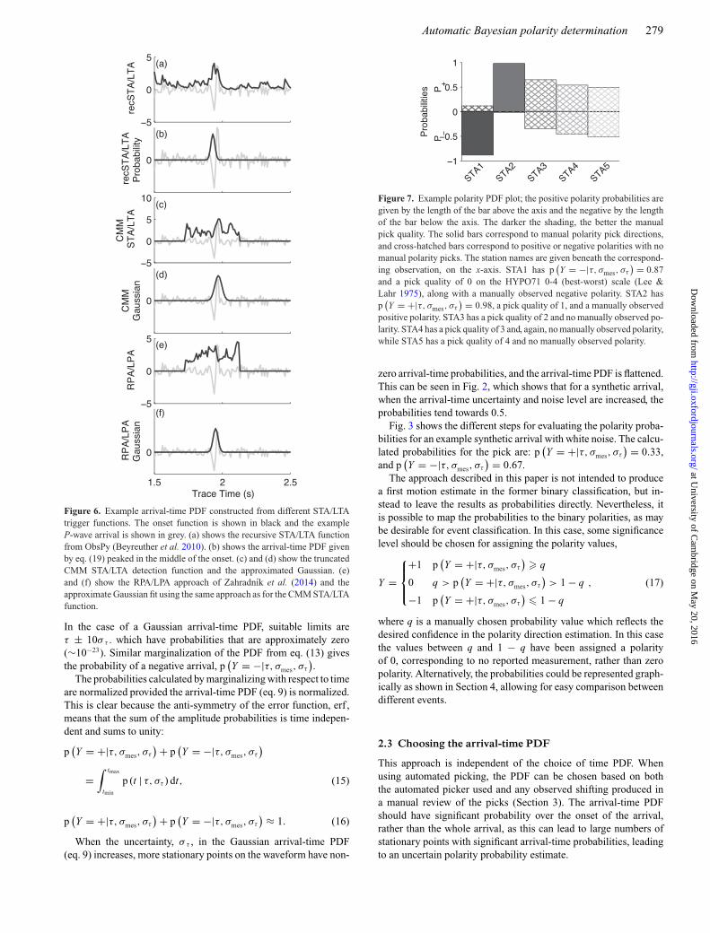
Figure 6. Example arrival-time PDF constructed from different STA/LTAtrigger functions. The onset function is shown in black and the exampleP-wave arrival is shown in grey. (a) shows the recursive STA/LTA functionfrom ObsPy (Beyreuther et al. 2010). (b) shows the arrival-time PDF givenby eq. (19) peaked in the middle of the onset. (c) and (d) show the truncatedCMM STA/LTA detection function and the approximated Gaussian. (e)and (f) show the RPA/LPA approach of Zahradnık et al. (2014) and theapproximate Gaussian fit using the same approach as for the CMM STA/LTAfunction.

In the case of a Gaussian arrival-time PDF, suitable limits areτ ± 10σ τ . which have probabilities that are approximately zero(∼10−23). Similar marginalization of the PDF from eq. (13) givesthe probability of a negative arrival, p

(Y = −|τ, σmes, στ

).

The probabilities calculated by marginalizing with respect to timeare normalized provided the arrival-time PDF (eq. 9) is normalized.This is clear because the anti-symmetry of the error function, erf ,means that the sum of the amplitude probabilities is time indepen-dent and sums to unity:


) + p(Y = −|τ, σmes, στ

)=

∫ tmax

tmin

p (t | τ, στ ) dt, (15)


) + p(Y = −|τ, σmes, στ

) ≈ 1. (16)

When the uncertainty, σ τ , in the Gaussian arrival-time PDF(eq. 9) increases, more stationary points on the waveform have non-

Figure 7. Example polarity PDF plot; the positive polarity probabilities aregiven by the length of the bar above the axis and the negative by the lengthof the bar below the axis. The darker the shading, the better the manualpick quality. The solid bars correspond to manual polarity pick directions,and cross-hatched bars correspond to positive or negative polarities with nomanual polarity picks. The station names are given beneath the correspond-ing observation, on the x-axis. STA1 has p


) = 0.87and a pick quality of 0 on the HYPO71 0-4 (best-worst) scale (Lee &Lahr 1975), along with a manually observed negative polarity. STA2 hasp

(Y = +|τ, σmes, στ

) = 0.98, a pick quality of 1, and a manually observedpositive polarity. STA3 has a pick quality of 2 and no manually observed po-larity. STA4 has a pick quality of 3 and, again, no manually observed polarity,while STA5 has a pick quality of 4 and no manually observed polarity.

zero arrival-time probabilities, and the arrival-time PDF is flattened.This can be seen in Fig. 2, which shows that for a synthetic arrival,when the arrival-time uncertainty and noise level are increased, theprobabilities tend towards 0.5.

Fig. 3 shows the different steps for evaluating the polarity proba-bilities for an example synthetic arrival with white noise. The calcu-lated probabilities for the pick are: p

(Y = +|τ, σmes, στ

) = 0.33,and p


) = 0.67.The approach described in this paper is not intended to produce

a first motion estimate in the former binary classification, but in-stead to leave the results as probabilities directly. Nevertheless, itis possible to map the probabilities to the binary polarities, as maybe desirable for event classification. In this case, some significancelevel should be chosen for assigning the polarity values,

Y =

⎧⎪⎨⎪⎩

+1 p(Y = +|τ, σmes, στ

)� q

0 q > p(Y = +|τ, σmes, στ

)> 1 − q

−1 p(Y = +|τ, σmes, στ

)� 1 − q

, (17)

where q is a manually chosen probability value which reflects thedesired confidence in the polarity direction estimation. In this casethe values between q and 1 − q have been assigned a polarityof 0, corresponding to no reported measurement, rather than zeropolarity. Alternatively, the probabilities could be represented graph-ically as shown in Section 4, allowing for easy comparison betweendifferent events.

2.3 Choosing the arrival-time PDF

This approach is independent of the choice of time PDF. Whenusing automated picking, the PDF can be chosen based on boththe automated picker used and any observed shifting produced ina manual review of the picks (Section 3). The arrival-time PDFshould have significant probability over the onset of the arrival,rather than the whole arrival, as this can lead to large numbers ofstationary points with significant arrival-time probabilities, leadingto an uncertain polarity probability estimate.

at University of C

ambridge on M


Dow

nloaded from



Figure 8. PDF plots for varying arrival-time picks on the same waveform.The original arrival-time pick is shown in (a), with randomly varied arrival-time picks in (b–f). The waveform is shown in grey, with the positive polarityPDF in red and the negative polarity PDF in blue. The vertical lines corre-spond to the arrival-time picks. The arrival-time picks were varied by addinga time shift randomly sampled from a Gaussian distribution.

Fig. 1 shows a histogram of P and S arrival-time shifts for thecoalescence microseismic mapping (CMM) autopicker (Drew et al.2005, 2013) for all pick weights. The mean shift is non-zero, likelydue to poor-quality picks that are improved manually and the CMMtendency to pick on the peak rather than the onset. Therefore, thechoice of a Gaussian probability around the CMM pick is not a poorone, although the mean could be chosen to be a small time shift (δt)before the automatic pick, to compensate for the CMM tendency topick slightly late:

p (t | τ, στ ) = 1√2πστ

2e− (t−τ+δt)2

2σ2τ . (18)

The arrival-time PDF must be arrival specific, so as to reflectthe confidence in the individual arrival-time estimate, although theshape could be derived from an empirical distribution of arrivaltimes for a subset of events in a data-set, such as that in Fig. 1, withthe width scaled by some measure of the arrival-time uncertainty.Alternatively, as discussed below, the arrival-time PDF can be based

on some characteristic function of the data, perhaps as used in anautomated picker (e.g. short-term averaging/long-term averaging,STA/LTA).

2.4 Manual and automated picking

This probabilistic approach produces an estimate of the likelihood ofthe polarity which can be combined with manual picking by usingthe manual observations as a prior probability for the automatedmeasurements. The choice of prior probability for the polarity canhave a large effect (Fig. 4). If the manual prior is large, the effect ofthe polarity probabilities is negligible, although as it is reduced tothe null prior (pprior = 0.5), the effect become more significant.

The prior has a strong effect, dominating the probabilities evenfor the incorrect polarity direction, but there is a clear difference inFig. 4 between the correct (negative) and incorrect (positive) priordirections, with a much sharper trend towards a value of 1 for theincorrect prior direction. Consequently, even if the prior probabilityis large and in the incorrect direction, the resultant polarity proba-bility for the correct direction will be larger than the correspondingprior probability value, and the probability is corrected towards thetrue value.

3 I N T E G R AT I O N W I T H AU T O M AT E DM O N I T O R I N G

The fast calculation speed allows this polarity estimation to be inte-grated into an automated processing workflow. This polarity infor-mation, in conjunction with other measurements such as amplituderatios, can produce an estimate of the event source, allowing forbetter data quality control from observations and helping to flag in-teresting events in near real time. The accuracy of such an approachstrongly depends on the accuracy of the arrival-time pick. As theerror is increased, the polarity probabilities will tend towards 0.5(Fig. 2). Therefore, provided the automated time picking is accurate,the polarity probabilities produced should show good consistencyand, although manual refinement could still improve the result, theresults from eq. (14) should improve the source constraints.

The arrival-time PDF can be based on some characteristic func-tion from the chosen automated picking method. The CMM eventdetection algorithm (Drew et al. 2013) uses an STA/LTA detectionfunction, which could be used as the arrival-time PDF in eqs (10)and (11). In CMM, the detection function is fitted with a Gaussianapproximation to produce an uncertainty estimate. However, Fig. 5shows that using the STA/LTA function (eq. 1, Drew et al. 2013) orits Gaussian approximation often produces wide arrival-time PDFs,encompassing most of the arrival rather than just the first motion.Furthermore, this detection function peaks away from the onset andleads to increased uncertainty in the pick time and, therefore, poorlydefined polarity probabilities. Both the Gaussian approximation andthe plain STA/LTA function show similar performance, providinglittle constraint on the polarity. Nevertheless, the maximum proba-bility (Fig. 5d) is in the negative direction, which is consistent withthe arrival (Fig. 5a).

Baer & Kradolfer (1987) introduced the concept of ‘phase detec-tors’ and ‘phase pickers’. Phase detectors are relatively imprecise,and will be improved by human re-picking. However, phase pickersshould produce results that are comparable to those picked manu-ally. Therefore, it may be better to use a phase picker to determinethe onset and construct the arrival-time PDF more accurately. Thereare many approaches to accurate onset pickers such as the methods

at University of C

ambridge on M


Dow

nloaded from



Figure 9. PDF plots for varying Gaussian and boxcar noise levels for the same waveform. The noise levels are: (a) No noise, (b) SNR = 10, (c) SNR = 5, (d)SNR = 3, (e) SNR = 2, and (f) SNR = 1.2. The waveform is shown in grey, with the positive polarity PDF in red and the negative polarity PDF in blue. Thevertical lines correspond to the arrival-time pick.

discussed by Baer & Kradolfer (1987): STA/LTA pickers (Allen1978, 1982; Trnkoczy 2012); auto-regressive pickers (Takanami &Kitagawa 1988, 1991; Nakamura 2004); stationary analysis pickers(Nakamula et al. 2007); kurtosis based pickers (Hibert et al. 2014;Ross & Ben-Zion 2014); right to left pick averaging (RPA/LPA)(Zahradnık et al. 2014), as well as many others. Withers et al. (1998)provide an overview of several of these different approaches, as doDi Stefano et al. (2006). Several of the STA/LTA-based approachesare shown in Fig. 6. Determining the parameters for these automatedpickers is not always straightforward, and parameters must often beadjusted based on the general signal characteristics (Trnkoczy 2012;Zahradnık et al. 2014).

Many of these approaches produce characteristic functions thathave a sharp increase at the onset (Ross & Ben-Zion 2014, fig. 3).So a possible definition of the arrival-time PDF could be a Gaussianusing the size and onset of the peak in the characteristic function(FC) as an indicator of the uncertainty, for example,

στ = τmax − τmin

FC (t = τmax) − FC (t = τmin), (19)

where τmax is the time of the maximum in the peak, and τmin is thetime of the minimum. Fig. 6(b) shows an example of this arrival-time PDF for a recursive STA/LTA pick, which is more focussedon the first arrival, rather than the whole of the arrival phase. Fig. 6shows that neither the CMM STA/LTA nor the RPA/LPA approachesis as good at resolving the arrival as the recursive STA/LTA method.

4 E X A M P L E S

In the following examples, manual arrival-time picks were madeon both the synthetic and real data. The arrival noise levels weremeasured in a time window from half way between the start of thetrace and the P-arrival. The exact window was constructed basedon the P arrival-time uncertainty so as to remove any significantprobability of any signal occurring in the noise window. The noiseestimate is important in eq. (14), but since the stationary pointsused in this approach are by definition at the extrema of the values,the result from eq. (7) is often close to 1 or 0 (Fig. 3b), so errors

at University of C

ambridge on M


Dow

nloaded from



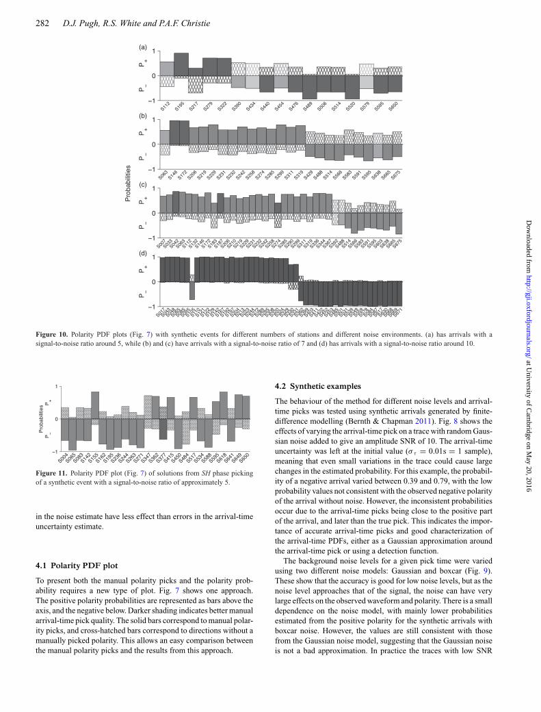
Figure 10. Polarity PDF plots (Fig. 7) with synthetic events for different numbers of stations and different noise environments. (a) has arrivals with asignal-to-noise ratio around 5, while (b) and (c) have arrivals with a signal-to-noise ratio of 7 and (d) has arrivals with a signal-to-noise ratio around 10.

Figure 11. Polarity PDF plot (Fig. 7) of solutions from SH phase pickingof a synthetic event with a signal-to-noise ratio of approximately 5.

in the noise estimate have less effect than errors in the arrival-timeuncertainty estimate.

4.1 Polarity PDF plot

To present both the manual polarity picks and the polarity prob-ability requires a new type of plot. Fig. 7 shows one approach.The positive polarity probabilities are represented as bars above theaxis, and the negative below. Darker shading indicates better manualarrival-time pick quality. The solid bars correspond to manual polar-ity picks, and cross-hatched bars correspond to directions without amanually picked polarity. This allows an easy comparison betweenthe manual polarity picks and the results from this approach.

4.2 Synthetic examples

The behaviour of the method for different noise levels and arrival-time picks was tested using synthetic arrivals generated by finite-difference modelling (Bernth & Chapman 2011). Fig. 8 shows theeffects of varying the arrival-time pick on a trace with random Gaus-sian noise added to give an amplitude SNR of 10. The arrival-timeuncertainty was left at the initial value (σ τ = 0.01s = 1 sample),meaning that even small variations in the trace could cause largechanges in the estimated probability. For this example, the probabil-ity of a negative arrival varied between 0.39 and 0.79, with the lowprobability values not consistent with the observed negative polarityof the arrival without noise. However, the inconsistent probabilitiesoccur due to the arrival-time picks being close to the positive partof the arrival, and later than the true pick. This indicates the impor-tance of accurate arrival-time picks and good characterization ofthe arrival-time PDFs, either as a Gaussian approximation aroundthe arrival-time pick or using a detection function.

The background noise levels for a given pick time were variedusing two different noise models: Gaussian and boxcar (Fig. 9).These show that the accuracy is good for low noise levels, but as thenoise level approaches that of the signal, the noise can have verylarge effects on the observed waveform and polarity. There is a smalldependence on the noise model, with mainly lower probabilitiesestimated from the positive polarity for the synthetic arrivals withboxcar noise. However, the values are still consistent with thosefrom the Gaussian noise model, suggesting that the Gaussian noiseis not a bad approximation. In practice the traces with low SNR

at University of C

ambridge on M


Dow

nloaded from



Table 1. Comparison of automated and manual polarity picks for the 2007/7/6 20:47 Upptyppingar event(White et al. 2011). Missing manual polarities are unpicked. Time pick qualities are manually assigned asgood or poor with associated time pick errors of 0.01 s and 0.5 s. These qualities would correspond to 0and 3 from the HYPO71 pick weighting (Lee & Lahr 1975). p(Y = +|τ, σmes, στ ) is the probability of apositive polarity and p(Y = −|τ, σmes, στ ) the probability of a negative polarity. The bolded probabilitiescorrespond to values larger than 0.6 which agree with the manual polarity pick for good (pick quality 0)picks.

Station Time pick quality Manual polarity p(Y = +|τ, σmes, στ

)p


)ADA Good + 0.94 0.06BRU Poor + 0.51 0.49DDAL Poor 0.50 0.50DYNG Poor – 0.50 0.50FREF Good – 0.19 0.81HELI Poor 0.50 0.50HERD Good + 0.70 0.30HETO Good + 0.90 0.10HOTT Good – 0.30 0.70HRUT Good + 0.99 0.01HVA Good + 0.94 0.06JOAF Poor 0.50 0.40KOLL Good + 0.65 0.35KRE Good – 0.06 0.94LOKA Good + 0.94 0.06MIDF Good – 0.30 0.70MKO Good – 0.06 0.94MOFO Good – 0.10 0.90MYVO Good + 0.70 0.30RODG Good – 0.30 0.70SVAD Good + 0.90 0.10UTYR Good – 0.09 0.91VADA Good – 0.30 0.70VIBR Good + 0.94 0.06VIKR Good 0.69 0.31VISA Poor 0.50 0.50VSH Good + 0.94 0.06

Figure 12. Polarity PDF plot (Fig. 7) for the 2007/07/06 20:47 event (Whiteet al. 2011) shown in Table 1.

(Figs 9d–f) would probably be considered difficult to pick and,therefore, be assigned a larger time pick error.

These examples also demonstrate why an arrival-time PDF withsome shift (eq. 18) may be better, as the arrival-time picks in Figs 8and 9 are closer to the onset rather than the first peak. Accordingly,the first motions are more likely to be after the pick time rather thanequally likely before and after.

As shown in these examples, the approach is robust and canprovide a qualitative value on the probability of the polarity beingup or down, but the probabilities are inherently dependent on theaccuracy of the arrival-time pick and the trace noise levels. Traceswith a high SNR should produce a reliable result, but as the time pickuncertainty increases, the polarity probability tends to 0.5 (Fig. 2).

Fig. 10 shows that the automated approach usually agrees withthe manually observed polarities, especially in the low-noise cases.However, as the noise levels increase, the solutions occasionally

Figure 13. Example polarity PDFs and waveform from the 2007/07/0620:47 event for station KRE. The positive polarity PDF is shown in red andthe negative polarity PDF is shown in blue and as negative for clarity. The(scaled) waveform is in grey; the P-arrival-time pick and manual polaritypick are indicated by the arrow. The time-marginalized automated polarityprobabilities are p(Y = +|τ, σmes, στ ) = 0.06 and p(Y = −|τ, σmes, στ ) =0.94.

disagree with the manually observed polarities, although this isexpected in the low-SNR examples.

This approach can also be used when evaluating S-phase po-larities, even though these require rotation into the correct rayorientation to measure them. Consequently, they cannot easilybe determined without an estimate of the hypocentre, unlike theP-wave polarities. Fig. 11 shows an example of SH-wave mea-surements from a synthetic event with an amplitude SNR of 5.The SH polarities were manually picked on the transverse compo-nent after the location was determined by rotating into the vertical,

at University of C

ambridge on M


Dow

nloaded from



Figure 14. Polarity PDF plots (Fig. 7) for example events from the Krafla central volcano in the Northern Volcanic Zone of Iceland.

radial and transverse (ZRT) components. The noise levels wereagain estimated by windowing before the arrival. For these observa-tions, any increased signal due to the P-arrival should be consideredas noise when estimating the SH-polarity probability, so the windowwas taken to include the P arrival time. The polarity probabilitiesshow good consistency with the manually picked polarities.

4.3 Real data

Table 1 shows a comparison between the automated and manualpolarity picks for one event from a July 2007 swarm beneath MountUpptyppingar in Iceland (White et al. 2011), with the polarity PDFplot shown in Fig. 12. The manual observations and automaticallydetermined solutions are consistent with good-quality arrival-timepicks producing probabilities larger than 0.7 and often larger than0.9. The poor picks with large time uncertainties show that theresulting probabilities tend to 0.5 each, as discussed in Section 2.Fig. 13 shows an example polarity PDF for one of the stations.

The results of the automated polarity picking for several eventsfrom the Krafla region of Iceland are shown in Fig. 14. For the mostpart, the automated polarity probabilities agree with the manualpolarities; although there a few cases that disagree; these are usuallycaused by an error in the manual arrival-time pick. This error madethe arrival-time PDF a poor approximation, often due to early or latepicks being assigned a high pick quality, leading to narrow arrival-time PDFs before or after the first arrival. The strong agreement ofthe observations suggests that this approach works well with realdata and not just with synthetically generated events.

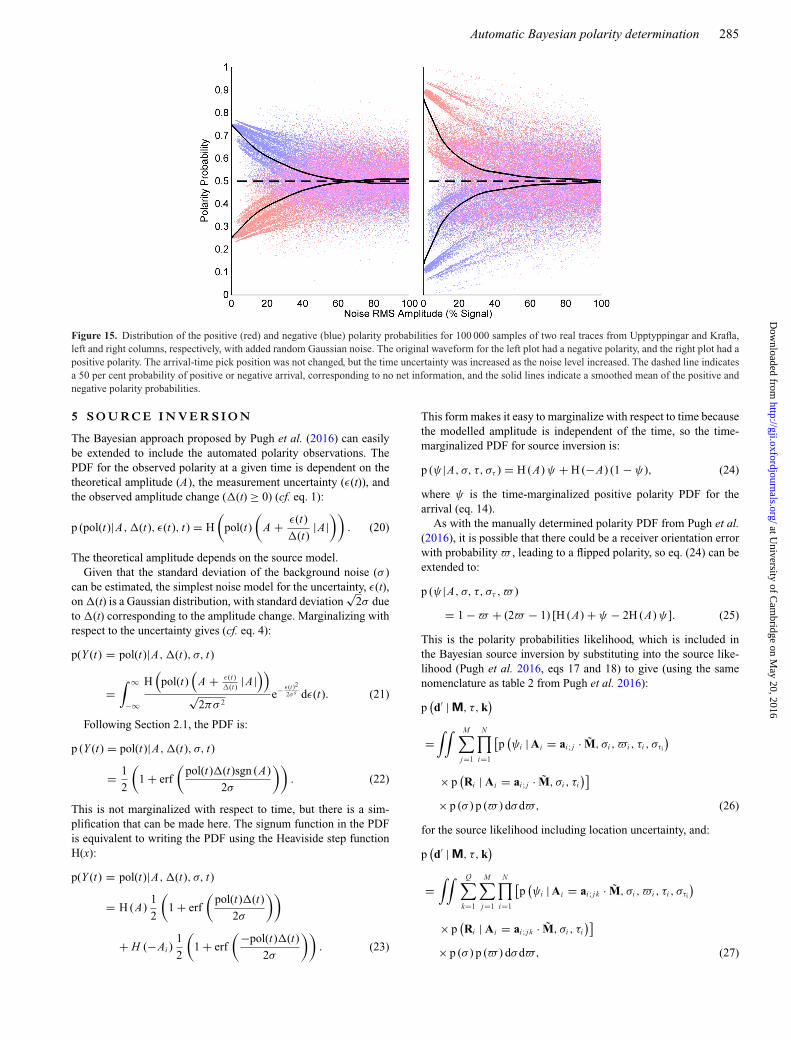
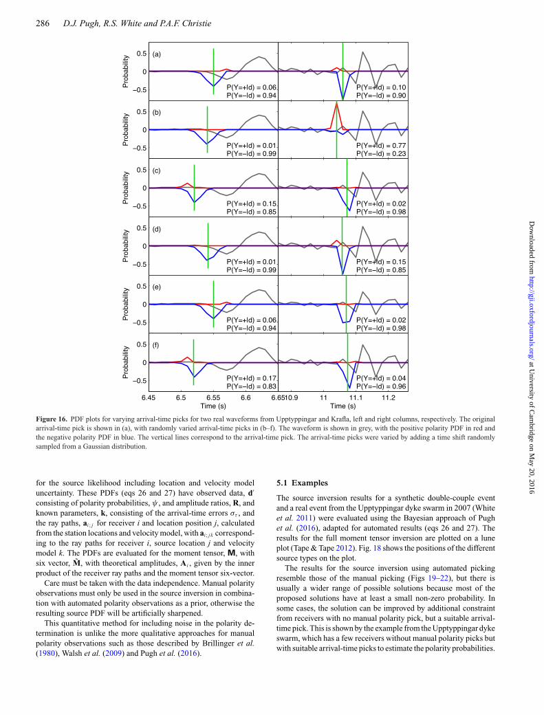
Fig. 15 shows the results from testing the polarity probabilityestimation with added noise levels on two traces from the Upptyp-pingar and Krafla data shown above. The results are consistent withthose shown in Fig. 2, although there is a faster decay to the 0.5probability line, and a wider spread of results, due to the more com-plex signal. Figs 16 and 17 show the effects of varying the time pickand noise level on the real data, and again the results are consistentwith those shown in Figs 8 and 9.

at University of C

ambridge on M


Dow

nloaded from



Figure 15. Distribution of the positive (red) and negative (blue) polarity probabilities for 100 000 samples of two real traces from Upptyppingar and Krafla,left and right columns, respectively, with added random Gaussian noise. The original waveform for the left plot had a negative polarity, and the right plot had apositive polarity. The arrival-time pick position was not changed, but the time uncertainty was increased as the noise level increased. The dashed line indicatesa 50 per cent probability of positive or negative arrival, corresponding to no net information, and the solid lines indicate a smoothed mean of the positive andnegative polarity probabilities.

5 S O U RC E I N V E R S I O N

The Bayesian approach proposed by Pugh et al. (2016) can easilybe extended to include the automated polarity observations. ThePDF for the observed polarity at a given time is dependent on thetheoretical amplitude (A), the measurement uncertainty (ε(t)), andthe observed amplitude change (�(t) ≥ 0) (cf. eq. 1):

p (pol(t)|A, �(t), ε(t), t) = H

(pol(t)

(A + ε(t)

�(t)|A|

)). (20)

The theoretical amplitude depends on the source model.Given that the standard deviation of the background noise (σ )

can be estimated, the simplest noise model for the uncertainty, ε(t),on �(t) is a Gaussian distribution, with standard deviation

√2σ due

to �(t) corresponding to the amplitude change. Marginalizing withrespect to the uncertainty gives (cf. eq. 4):

p(Y (t) = pol(t)|A, �(t), σ, t)

=∫ ∞

−∞

H(

pol(t)(

A + ε(t)�(t)

|A|))

√2πσ 2

e− ε(t)2

2σ s dε(t). (21)

Following Section 2.1, the PDF is:

p (Y (t) = pol(t)|A, �(t), σ, t)

= 1

2

(1 + erf

(pol(t)�(t)sgn (A)

2σ

)). (22)

This is not marginalized with respect to time, but there is a sim-plification that can be made here. The signum function in the PDFis equivalent to writing the PDF using the Heaviside step functionH(x):

p(Y (t) = pol(t)|A, �(t), σ, t)

= H (A)1

2

(1 + erf

(pol(t)�(t)

2σ

))

+ H (−Ai )1

2

(1 + erf

(−pol(t)�(t)

2σ

)). (23)

This form makes it easy to marginalize with respect to time becausethe modelled amplitude is independent of the time, so the time-marginalized PDF for source inversion is:

p (ψ |A, σ, τ, στ ) = H (A) ψ + H (−A) (1 − ψ), (24)

where ψ is the time-marginalized positive polarity PDF for thearrival (eq. 14).

As with the manually determined polarity PDF from Pugh et al.(2016), it is possible that there could be a receiver orientation errorwith probability , leading to a flipped polarity, so eq. (24) can beextended to:

p (ψ |A, σ, τ, στ , )

= 1 − + (2 − 1) [H (A) + ψ − 2H (A) ψ]. (25)

This is the polarity probabilities likelihood, which is included inthe Bayesian source inversion by substituting into the source like-lihood (Pugh et al. 2016, eqs 17 and 18) to give (using the samenomenclature as table 2 from Pugh et al. 2016):

p(d′ | M, τ, k

)

=∫∫ M∑

j=1

N∏i=1

[p

(ψi | Ai = ai ; j · M, σi , i , τi , στi

)

× p(Ri | Ai = ai ; j · M, σi , τi

)]× p (σ ) p ( ) dσd, (26)

for the source likelihood including location uncertainty, and:

p(d′ | M, τ, k

)

=∫∫ Q∑

k=1

M∑j=1

N∏i=1

[p

(ψi | Ai = ai ; jk · M, σi ,i , τi , στi

)

× p(Ri | Ai = ai ; jk · M, σi , τi

)]× p (σ ) p ( ) dσd, (27)

at University of C

ambridge on M


Dow

nloaded from



Figure 16. PDF plots for varying arrival-time picks for two real waveforms from Upptyppingar and Krafla, left and right columns, respectively. The originalarrival-time pick is shown in (a), with randomly varied arrival-time picks in (b–f). The waveform is shown in grey, with the positive polarity PDF in red andthe negative polarity PDF in blue. The vertical lines correspond to the arrival-time pick. The arrival-time picks were varied by adding a time shift randomlysampled from a Gaussian distribution.

for the source likelihood including location and velocity modeluncertainty. These PDFs (eqs 26 and 27) have observed data, d′

consisting of polarity probabilities, ψ , and amplitude ratios, R, andknown parameters, k, consisting of the arrival-time errors στ , andthe ray paths, ai ; j for receiver i and location position j, calculatedfrom the station locations and velocity model, with ai ; jk correspond-ing to the ray paths for receiver i, source location j and velocitymodel k. The PDFs are evaluated for the moment tensor, M, withsix vector, M, with theoretical amplitudes, Ai , given by the innerproduct of the receiver ray paths and the moment tensor six-vector.

Care must be taken with the data independence. Manual polarityobservations must only be used in the source inversion in combina-tion with automated polarity observations as a prior, otherwise theresulting source PDF will be artificially sharpened.

This quantitative method for including noise in the polarity de-termination is unlike the more qualitative approaches for manualpolarity observations such as those described by Brillinger et al.(1980), Walsh et al. (2009) and Pugh et al. (2016).

5.1 Examples

The source inversion results for a synthetic double-couple eventand a real event from the Upptyppingar dyke swarm in 2007 (Whiteet al. 2011) were evaluated using the Bayesian approach of Pughet al. (2016), adapted for automated results (eqs 26 and 27). Theresults for the full moment tensor inversion are plotted on a luneplot (Tape & Tape 2012). Fig. 18 shows the positions of the differentsource types on the plot.

The results for the source inversion using automated pickingresemble those of the manual picking (Figs 19–22), but there isusually a wider range of possible solutions because most of theproposed solutions have at least a small non-zero probability. Insome cases, the solution can be improved by additional constraintfrom receivers with no manual polarity pick, but a suitable arrival-time pick. This is shown by the example from the Upptyppingar dykeswarm, which has a few receivers without manual polarity picks butwith suitable arrival-time picks to estimate the polarity probabilities.

at University of C

ambridge on M


Dow

nloaded from



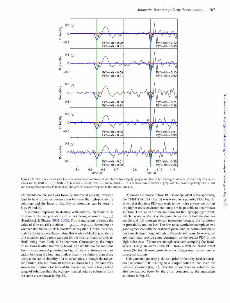
Figure 17. PDF plots for varying Gaussian noise levels on two real waveforms from Upptyppingar and Krafla, left and right columns, respectively. The noiselevels are: (a) SNR = 10, (b) SNR = 5, (c) SNR = 3, (d) SNR = 2, and (e) SNR = 1.2. The waveform is shown in grey, with the positive polarity PDF in redand the negative polarity PDF in blue. The vertical lines correspond to the arrival-time pick.

The double-couple solutions from the automated polarity inversiontend to have a clearer demarcation between the high-probabilitysolutions and the lower-probability solutions, as can be seen inFigs 19 and 20.

A common approach to dealing with polarity uncertainties isto allow a blanket probability of a pick being incorrect (pmispick)(Hardebeck & Shearer 2002, 2003). This is equivalent to setting thevalue of ψ in eq. (25) to either 1 − pmispick or pmispick depending onwhether the manual pick is positive or negative. Unlike the auto-mated polarity approach, including this arbitrary blanket probabilityof a mistaken pick cannot account for the most-difficult-to-pick ar-rivals being most likely to be incorrect. Consequently, the rangeof solutions is often not overly broad. The double-couple solutionsfrom the automated polarities in Fig. 20 show a stronger demar-cation between the low- and high-probability solutions than thoseusing a blanket probability of a mistaken pick, although the rangesare similar. The full moment tensor solutions in Fig. 20 have verysimilar distributions for both of the inversions, with a less peakedrange of solutions than the ordinary manual polarity solutions fromthe same event shown in Fig. 19.

Although the choice of time PDF is independent of the approach,the CMM STA/LTA (Fig. 5) was tested as a possible PDF. Fig. 21shows that this time PDF can work in low-noise environments, butin a higher-noise environment it may not be possible to determine asolution. This is clear in the solutions for the Upptyppingar event,which has no constraint on the possible source for both the double-couple and full moment tensor inversions because the variationsin probability are too low. The low-noise synthetic example showsgood agreement with the east-west plane, but the north-south planehas a much larger range of high probability solutions. However, theapproach may provide some constraint on the source PDF in thehigh-noise case if there are enough receivers sampling the focal-sphere. Using an arrival-time PDF from a well calibrated onsetpicker (Section 3) would provide a much larger improvement in thesource constraints.

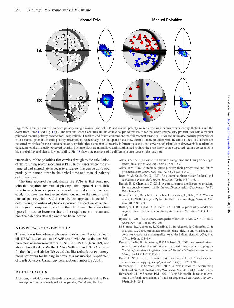
Using manual polarity picks as a prior probability further sharp-ens the source PDF, leading to a sharper solution than even themanual polarities (Fig. 22). The full moment tensor solutions arealso constrained better by the prior, compared to the equivalentsolutions in Fig. 19.

at University of C

ambridge on M


Dow

nloaded from



Figure 18. Example of the fundamental eigenvalue lune (Tape & Tape2012), showing the position of the different source types. The horizontalaxis corresponds to the eigenvalue longitude γ

(− π6 � γ � π

6

)and the

vertical axis, the eigenvalue latitude δ(− π

2 � δ � π2

). The double-couple

point (DC) lies at the intersection of the two lines. TC+ and TC− correspondto the opening and closing variants of the tensile crack model (Shimizu et al.1987). The two compensated linear vector dipole (CLVD) sources (Knopoff& Randall 1970) are also shown on the plot.

6 S U M M A RY A N D D I S C U S S I O N

The Bayesian approach to automated polarity determination pro-posed in this paper is a quantitative approach that enables rigorousincorporation of measurement uncertainties into the polarity prob-ability estimates. It is an alternative approach to the traditional bi-nary classification of polarities, and can be adapted for use with any

onset or arrival-time picking method, either manual or automatic.The polarity probabilities estimated using this method provide aquantitative approach for including the polarity uncertainties in thesource inversion. This contrasts with many common approaches,including the qualitative approach for manual polarity observationdescribed by Brillinger et al. (1980), Walsh et al. (2009) and Pughet al. (2016), and the arbitrarily determined probability of a mistakenpick (Hardebeck & Shearer 2002, 2003).

The polarity probabilities have a clear dependence on the timepick accuracy and the noise level of the trace, requiring an accu-rate arrival-time pick. Poorly characterized arrival-time pick un-certainties lead to little discrimination in the polarity probabilities.Consequently, when an automated arrival picking approach is used,accurate onset picks with results comparable to picks made by a hu-man are required, otherwise the resultant arrival-time PDF is usuallytoo wide.

The choice of arrival-time PDF can be adjusted depending onthe perceived quality of the arrival time picking approach. For anautomated picker, the arrival-time PDF peak can be shifted to justbefore the pick if the automated pick tends to be late, as is the casefor the CMM STA/LTA picker. The arrival-time PDF can also beadjusted using the pick quality estimate, such as the pick weight(0–4 range from HYPO71 Lee & Lahr 1975), although a range withfiner discretization would prove more accurate.

In the real-world cases from the Upptyppingar volcano and Kraflain Iceland, there are few differences between the results obtainedfrom manual and automated picking. The estimation of the proba-bility of correct first motions produces a quantitative estimate of the

Figure 19. Comparison between automated polarity and manual polarity source inversions for two events, one synthetic (a) and the event from Table 1and Fig. 12(b). The first and second columns are the double-couple source PDFs for the automated polarity probabilities and manual polarity observations,respectively. The third and fourth columns are the full moment tensor PDFs for the automated polarity probabilities and manual polarity observations,respectively. The fault plane plots show the most likely solutions with the darkest lines. The stations are indicated by circles for the automated polarityprobabilities, as no manual polarity information is used, and upwards red triangles or downwards blue triangles depending on the manually observed polarity.The lune plots are normalized and marginalized to show the most likely source type; red regions correspond to high probability and blue to low probability.Fig. 18 shows the positions of the different source types on the lune plot.

at University of C

ambridge on M


Dow

nloaded from



Figure 20. Comparison of automated polarity and arbitrary probability of a mistaken pick(

pmispick = 0.1)

for two events, one synthetic (a) and the eventfrom Table 1 and Fig. 12(b). The first and second columns are the double-couple source PDFs for the automated polarity probabilities and manual polarityobservations with mispick, respectively. The third and fourth columns are the full moment tensor PDFs for the automated polarity probabilities and manualpolarity observations with mispick, respectively. The fault plane plots show the most likely solutions with the darkest lines. The stations are indicated by circlesif there is no manual polarity information used, and upwards red triangles or downwards blue triangles depending on the manually observed polarity. The luneplots are normalized and marginalized to show the most likely source type; red regions correspond to high probability and blue to low probability. Fig. 18shows the positions of the different source types on the lune plot.

Figure 21. Comparison of automated polarity using a Gaussian time PDF around the manual time pick and STA/LTA time picking for two events, one synthetic(a) and the event from Table 1 and Fig. 12(b). The first and second columns are the double-couple source PDFs for the Gaussian time PDF and the STA/LTAtime PDF, respectively. The third and fourth columns are the full moment tensor PDFs for the Gaussian time PDF and the STA/LTA time PDF, respectively.The fault plane plots show the most likely solutions with the darkest lines. The stations are indicated by circles for the automated polarity probabilities, as nomanual polarity information is used, and upwards red triangles or downwards blue triangles depending on the manually observed polarity. The lune plots arenormalized and marginalized to show the most likely source type; red regions correspond to high probability and blue to low probability. Fig. 18 shows thepositions of the different source types on the lune plot.

at University of C

ambridge on M


Dow

nloaded from



Figure 22. Comparison of automated polarity using a manual prior of 0.85 and manual polarity source inversions for two events, one synthetic (a) and theevent from Table 1 and Fig. 12(b). The first and second columns are the double-couple source PDFs for the automated polarity probabilities with a manualprior and manual polarity observations, respectively. The third and fourth columns are the full moment tensor PDFs for the automated polarity probabilitieswith a manual prior and manual polarity observations, respectively. The fault plane plots show the most likely solutions with the darkest lines. The stations areindicated by circles for the automated polarity probabilities, as no manual polarity information is used, and upwards red triangles or downwards blue trianglesdepending on the manually observed polarity. The lune plots are normalized and marginalized to show the most likely source type; red regions correspond tohigh probability and blue to low probability. Fig. 18 shows the positions of the different source types on the lune plot.

uncertainty of the polarities that carries through to the calculationof the resulting source mechanism PDF. In the cases where the au-tomated and manual picks seem to disagree, this can be attributedpartially to human error in the arrival time and manual polaritydeterminations.

The time required for calculating the PDFs is fast comparedwith that required for manual picking. This approach adds littletime to an automated processing workflow, and can be includedeasily into near-real-time event detection, unlike the much slowermanual polarity picking. Additionally, the approach is useful fordetermining polarities of phases measured on location-dependentseismogram components, such as the SH phase. These are oftenignored in source inversion due to the requirement to return andpick the polarities after the event has been located.

A C K N OW L E D G E M E N T S

This work was funded under a Natural Environment Research Coun-cil (NERC) studentship as a CASE award with Schlumberger. Seis-mometers were borrowed from the NERC SEIS-UK (loan 842), whoalso archive the data. We thank Mike Williams and Chris Chapmanfor their help and advice. We would also like to thank our two anony-mous reviewers for helping improve this manuscript. Departmentof Earth Sciences, Cambridge contribution number ESC3601.

R E F E R E N C E S

Aldersons, F., 2004. Toward a three-dimensional crustal structure of the DeadSea region from local earthquake tomography, PhD thesis, Tel Aviv.

Allen, R.V., 1978. Automatic earthquake recognition and timing from singletraces, Bull. seism. Soc. Am., 68(5), 1521–1532.

Allen, R.V., 1982. Automatic phase pickers: their present use and futureprospects, Bull. seism. Soc. Am., 72(6B), S225–S242.

Baer, M. & Kradolfer, U., 1987. An automatic phase picker for local andteleseismic events, Bull. seism. Soc. Am., 77(4), 1437–1445.

Bernth, H. & Chapman, C., 2011. A comparison of the dispersion relationsfor anisotropic elastodynamic finite-difference grids, Geophysics, 76(3),WA43–WA50.

Beyreuther, M., Barsch, R., Krischer, L., Megies, T., Behr, Y. & Wasser-mann, J., 2010. ObsPy: a Python toolbox for seismology, Seismol. Res.Lett., 81, 530–533.

Brillinger, D.R., Udias, A. & Bolt, B.A., 1980. A probability model forregional focal mechanism solutions, Bull. seism. Soc. Am., 70(1), 149–170.

Byerly, P., 1926. The Montana earthquake of June 28, 1925, G.M.C.T., Bull.seism. Soc. Am., 16(4), 209–265.

Di Stefano, R., Aldersons, F., Kissling, E., Baccheschi, P., Chiarabba, C. &Giardini, D., 2006. Automatic seismic phase picking and consistent ob-servation error assessment: application to the Italian seismicity, Geophys.J. Int., 165(1), 121–134.

Drew, J., Leslie, D., Armstrong, P. & Michaud, G., 2005. Automated micro-seismic event detection and location by continuous spatial mapping, inSociety of Petroleum Engineers Annual Technical Conference and Exhi-bition, doi:10.2118/95513-MS.

Drew, J., White, R.S., Tilmann, F. & Tarasewicz, J., 2013. Coalescencemicroseismic mapping, Geophys. J. Int., 195(3), 1773–1785.

Hardebeck, J.L. & Shearer, P.M., 2002. A new method for determiningfirst-motion focal mechanisms, Bull. seism. Soc. Am., 92(6), 2264–2276.

Hardebeck, J.L. & Shearer, P.M., 2003. Using S/P amplitude ratios to con-strain the focal mechanisms of small earthquakes, Bull. seism. Soc. Am.,93(6), 2434–2444.

at University of C

ambridge on M


Dow

nloaded from



Hibert, C. et al., 2014. Automated identification, location, and volume es-timation of rockfalls at Piton de la Fournaise volcano, J. geophys. Res.,119, 1082–1105.

Knopoff, L. & Randall, M.J., 1970. The compensated linear-vector dipole:a possible mechanism for deep earthquakes, J. geophys. Res., 75(26),4957–4963.

Lee, W.H.K. & Lahr, J.C., 1975. HYPO71 (Revised): a computer programfor determining hypocenter, magnitude and first motion pattern of localearthquakes, Tech. Rep. 300, USGS.

Nakamula, S., Takeo, M., Okabe, Y. & Matsuura, M., 2007. Automaticseismic wave arrival detection and picking with stationary analysis: ap-plication of the KM2O-Langevin equations, Earth Planets Space, 59(6),567–577.

Nakamura, M., 2004. Automatic determination of focal mechanism solu-tions using initial motion polarities of P and S waves, Phys. Earth planet.Inter., 146(3-4), 531–549.

Nakano, H., 1923. Notes on the nature of the forces which give rise to theearthquake motions, Seismol. Bull. Cent. Met. Obs. Japan, 1, 92–120.

Pugh, D.J., White, R.S. & Christie, P.A.F., 2016. A Bayesian method formicroseismic source inversion, Geophys. J. Int., (submitted).

Reasenberg, P.A. & Oppenheimer, D., 1985. FPFIT, FPPLOT and FPPAGE:Fortran computer programs for calculating and displaying earthquakefault-plane solutions - OFR 85-739, Tech. rep., USGS.

Ross, Z.E. & Ben-Zion, Y., 2014. Automatic picking of direct P, S seismicphases and fault zone head waves, Geophys. J. Int., 199(1), 368–381.

Shimizu, H., Ueki, S. & Koyama, J., 1987. A tensile-shear crack model forthe mechanism of volcanic earthquakes, Tectonophysics, 144, 287–300.

Sivia, D.S., 2000. Data Analysis: A Bayesian Tutorial, Oxford Univ. Press.Snoke, J.A., 2003. FOCMEC: FOCal MEChanism determinations, Tech.

rep.Takanami, T. & Kitagawa, G., 1988. A new efficient procedure for

the estimation of onset times of seismic waves, J. Phys. Earth, 36,267–290.

Takanami, T. & Kitagawa, G., 1991. Estimation of the arrival times ofseismic waves by multivariate time series model, Ann. Inst. Stat. Math.,43(3), 403–433.

Tape, W. & Tape, C., 2012. A geometric setting for moment tensors, Geo-phys. J. Int., 190(1), 476–498.

Trnkoczy, A., 2012. Understanding and parameter setting of STA/LTA trig-ger algorithm, in New Manual of Seismological Observatory Practice 2(NMSOP-2), pp. 1–20, ed. Bormann, P., Deutsches GeoForschungsZen-trum GFZ.

Walsh, D., Arnold, R. & Townend, J., 2009. A Bayesian approach to deter-mining and parametrizing earthquake focal mechanisms, Geophys. J. Int.,176(1), 235–255.

White, R.S., Drew, J., Martens, H.R., Key, J., Soosalu, H. & Jakobsdottir,S.S., 2011. Dynamics of dyke intrusion in the mid-crust of Iceland, Earthplanet. Sci. Lett., 304(3–4), 300–312.

Withers, M., Aster, R., Young, C., Beiriger, J., Harris, M., Moore, S. &Trujillo, J., 1998. A comparison of select trigger algorithms for automatedglobal seismic phase and event detection, Bull. seism. Soc. Am., 88(1),95–106.

Zahradnık, J., Jansky, J. & Plicka, V., 2014. Analysis of the source scanningalgorithm with a new P-wave picker, J. Seismol., 19(2), 423–441.

at University of C

ambridge on M


Dow

nloaded from


Documents

Geophysical Journal International - ESC Publicationseprints.esc.cam.ac.uk/3601/7/Geophys. J. Int.-2016-Pugh-275-91.pdfGeophysical Journal International Geophys. J. Int. (2016) 206,