Geophysicae Tidal variations of O Atmospheric and OH(6-2

Annales Geophysicae, 23, 3579–3590, 2005SRef-ID: 1432-0576/ag/2005-23-3579© European Geosciences Union 2005

AnnalesGeophysicae

Tidal variations of O2 Atmospheric and OH(6-2) airglow andtemperature at mid-latitudes from SATI observations

M. J. L opez-Gonzalez1, E. Rodrıguez1, G. G. Shepherd2, S. Sargoytchev2, M. G. Shepherd2, V. M. Aushev3,S. Brown2, M. Garcıa-Comas1, and R. H. Wiens4

1Instituto de Astrofısica de Andalucıa, CSIC, P.O. Box 3004, E-18080 Granada, Spain2Centre for Research in Earth and Space Science, York University, 4700 Keele St., Toronto, Ontario M3J 1P3, Canada3Institute of Ionosphere, Ministry of Education and Science, Almaty, 480020, Kazakhstan4Department of Physics, University of Asmara, Eritrea, N. E. Africa

Received: 16 September 2005 – Revised: 18 October 2005 – Accepted: 27 October 2005 – Published: 23 December 2005

Abstract. Airglow observations with a Spectral AirglowTemperature Imager (SATI), installed at the Sierra NevadaObservatory (37.06◦ N, 3.38◦ W) at 2900-m height, havebeen used to investigate the presence of tidal variations atmid-latitudes in the mesosphere/lower thermosphere region.Diurnal variations of the column emission rate and verticallyaveraged temperature of the O2 Atmospheric (0-1) band andof the OH Meinel (6-2) band from 5 years (1998–2003) ofobservations have been analysed. From these observationsa clear tidal variation of both emission rates and rotationaltemperatures is inferred. It is found that the amplitude ofthe daily variation for both emission rates and temperaturesis greater from late autumn to spring than during summer.The amplitude decreases by more than a factor of two dur-ing summer and early autumn with respect to the amplitudein the winter-spring months. Although the tidal modulationsare preferentially semidiurnal in both rotational temperaturesand emission rates during the whole year, during early springthe tidal modulations seem to be more consistent with a di-urnal modulation in both rotational temperatures and emis-sion rates. Moreover, the OH emission rate from late au-tumn to early winter has a pattern suggesting both diurnaland semidiurnal tidal modulations.

Keywords. Atmospheric composition and structure (Air-glow and aurora; pressure density and temperature; instru-ments and techniques)

1 Introduction

Airglow emissions have been used to study the chemicaland dynamical behaviour of the atmosphere in those regions

Correspondence to:M. J. Lopez-Gonzalez([email protected])

where the emission takes place. Atmospheric tides are theglobal response of the atmosphere to the periodic forcing ofsolar heating. The influence of the atmospheric tides on theairglow emissions has been studied since 1970 (e.g. Wiensand Weill, 1973; Petitdidier and Teitelbaum, 1977; Takahashiet al., 1977). The tides present periodicities equal to the so-lar day and its harmonics, and propagate westward followingthe motion of the Sun (e.g.Chapman and Lindzen, 1970).

There is an enormous body of ground-based observationsof the mesosphere and lower thermosphere by the globalradar network (e.g. Jacobi et al., 1999; Pancheva et al., 2000,2002; Riggin et al., 2003; Forbes et al., 2004; Manson etal., 2004; Portnyagin et al., 2004) that have been used tostudy the tidal behaviour of the atmospheric winds. Stud-ies of the influences of atmospheric tides on airglow emis-sion and temperature using long-term, ground-based obser-vations (e.g. Wiens and Weill, 1973; Petitdidier and Teitel-baum, 1977; Scheer and Reisin, 1990; Reisin and Scheer,1996; Takahashi et al., 1998; Choi et al., 1998) and satelliteairglow observations (Abreu and Yee, 1989; Burrage et al.,1994; Shepherd et al., 1995, 1998) have shown a large vari-ation in diurnal behaviour of the airglow emission rates as afunction of the year and of the latitude.

Simultaneous satellite observations of emission rates, tem-peratures and winds performed with the High ResolutionDoppler Imager (HRDI) and Wind Imaging Interferometer(WINDII), both on board the UARS satellite, have been usedto study the tidal variations in airglow emission rates andwinds (Burrage et al., 1994; Shepherd et al., 1995, 1998;Shepherd et al., 2004a).

Here, we analysed the tidal variation found from long-term, ground-based airglow observations at 37.06◦ N lati-tude. These observations have been made by a SpectralAirglow Temperature Imager (SATI) instrument placed atthe Sierra Nevada Observatory. This instrument is able to

3580 M. J. Lopez-Gonzalez et al.: Tidal airglow variations at mid-latitudes

measure the column emission rate and the vertically aver-aged rotational temperature of both the O2 Atmospheric (0-1) band, and the OH Meinel (6-2) band, using the techniqueof interference filter spectral imaging with a cooled CCD de-tector (Wiens et al., 1997). The data analysed cover a periodfrom 1998 to 2003. Tidal variations of the temperature andairglow emission rates of the O2 Atmospheric (0-1) band andthe OH Meinel (6-2) band are presented and compared withprevious results. It is shown that the diurnal variation of theemission rates and temperatures has a seasonal dependence.The amplitudes of the variations observed during late autumnto spring are greater by more than a factor of two than thoseobserved during the rest of the year.

2 Observations

SATI is installed at the Sierra Nevada Observatory (37.06◦ N,3.38◦ W), Granada, Spain, at 2900-m height. It has been incontinuous operation since October 1998. SATI is a spatialand spectral imaging Fabry-Perot spectrometer in which theetalon is a narrow band interference filter and the detectoris a CCD camera. The SATI instrumental concept and opti-cal configuration was originally developed as the MesopauseOxygen Rotational Temperature Imager (MORTI) instru-ment (Wiens et al., 1991). The new adaptation as SATI isdescribed in detail bySargoytchev et al.(2004). The instru-ment uses two interference filters, one centred at 867.689 nm(in the spectral region of the O2 Atmospheric (0-1) band) andthe second one centred at 836.813 nm (in the spectral regionof the OH Meinel (6-2) band). Its field of view is an annu-lus of 30◦ average radius and 7.1◦ angular width, centeredon the zenith. Thus, an annulus of average radius of 55 kmand 16 km width at 95 km (or an average radius of 49 km and14 km width at 85 km) is observed in the sky.

The images are disks where the polar angle dimension cor-responds to the azimuth of the ring of the sky observed, whilethe radial distribution of the images contains the spectral dis-tribution, from which the rotational temperature is inferred.The method of SATI image reduction and temperature andemission rate determination was described in detail by Wienset al. (1991) for the O2 Atmospheric system, and byLopez-Gonzalez et al.(2004) for the OH(6-2) Meinel band.

In this work the images obtained from SATI are analysedas a whole, obtaining an average of the rotational temperatureand emission rate of the airglow band from the whole skyring.

The seasonal variation in rotational temperatures and air-glow emission rates measured with the SATI instrument dur-ing the period of October 1998 to March 2002 have beenanalysed and presented byLopez-Gonzalez et al.(2004). Inthe current study new data from March 2002 to May 2003have been added to the earlier data set and are analysed,in order to derive the tidal variations present in both rota-tional temperatures and emission rates. The OH tempera-tures deduced from the Q-branch have been corrected from

the error introduced by using Q-branch theoretical Einsteincoefficients (seePendleton and Taylor, 2002).

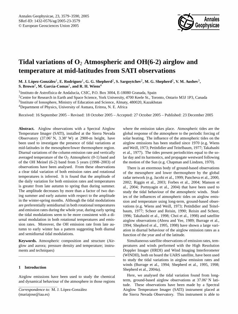
Table 1 shows the number of days and hours of observationused in the study, in each month from October 1998 to May2003. Table 1 also shows the total number of days and hoursper month. We have used all the data corresponding to goodobserving conditions, even data corresponding to short daysof observations, with the aim of obtaining the largest amountof data.

There are months, such as January 1999, when only twoshort nights of data are available, and the nocturnal variationof this month covers only one-third of the night comparedwith January data of other years. However, although onlyone-third of the night was covered, a strong correlation ex-isted with the nocturnal variation during this one-third of thenight and that obtained during the January nights of otheryears.

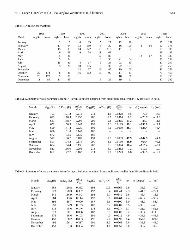
Lopez-Gonzalez et al.(2004) have shown that rotationaltemperatures and emission rates have a marked short-termvariability together with a clear seasonal variation. Tables 2and 3 show the mean rotational temperatures (TO2 andTOH)and emission rates (EO2 andEOH) for each month of the yeardue to the seasonal variation of these parameters found inSATI data. In Tables 2 and 3 are also listed other quanti-ties that will be discussed in the following section: the abso-lute amplitudes of the temperature and emission rate varia-tions (1TO2, 1TOH, 1EO2 and1EOH), the relative temper-

ature and emission rate amplitudes, (1TO2TO2

, 1TOHTOH

,1EO2EO2

and

1EOHEOH

), the amplitudes and phases of the Krassovsky ratio

(|η|,φ) and the vertical wavelengths (λz) for the propagationof the tidal modulations found from both emissions.

Here our interest is to determine the tidal variations and theseasonal dependences of these tidal variations. First of all,we subtracted the annual and semiannual seasonal variationsin the rotational temperature and emission rates of both OHand O2 emissions (see Tables 2 and 3). Here we employ theresidual temperatures and emission rates after removing theseasonal dependences.

For the systematic organization of the data we averagethese residual rotational temperatures and emission ratesfrom each night over 30-min intervals, centered on the hoursand half hours. Thus, an averaged nighttime variation is ob-tained for each night of available data, for every night of themonth. This reduces short-period variations but does not af-fect tidal components. By averaging the values obtained atthe same local time over one month, we obtain the diurnalvariation for each month of available observations in eachyear of SATI observations. A “mean” monthly diurnal vari-ation is then derived by averaging the monthly diurnal varia-tions over the 5-year period.

3 Results

The averaged diurnal variations, for each month, from 1998to 2003, together with the “mean” diurnal variation, are

M. J. Lopez-Gonzalez et al.: Tidal airglow variations at mid-latitudes 3581

Table 1. Airglow observations.

1998 1999 2000 2001 2002 2003 TotalMonth nights hours nights hours nights hours nights hours nights hours nights hours nights hours

January 2 7 6 23 5 27 12 90 25 151February 17 94 13 150 3 20 16 109 8 69 57 373March 15 93 14 122 19 119 11 62 59 396April 9 69 9 58 11 63 29 193May 5 36 12 80 12 67 29 183June 5 34 8 36 21 84 38 154July 15 81 4 17 5 24 23 85 47 207August 5 20 18 105 6 30 22 103 51 258September 12 67 12 85 19 100 43 252October 22 174 6 36 16 112 18 90 11 43 73 455November 23 172 9 88 18 98 50 358December 11 86 11 89 6 26 19 91 47 292

Table 2. Summary of wave parameters from OH layer. Solutions obtained from amplitudes smaller than 3 K are listed in bold.

Month EOH(R) 1EOH (R) 1EOHEOH

TOH(K) 1TOH (K) 1TOHTOH

|η| φ (degree) λz (km)

January 793 171.2 0.216 211 4.8 0.0228 9.5 −77.9 −14.3February 692 178.3 0.258 208 6.5 0.0314 8.2 −70.7 −17.0March 637 188.7 0.296 205 5.4 0.0265 11.2 −88.7 −11.8April 652 160.9 0.247 199 2.6 0.0129 19.1 −158.9 −19.1May 690 151.8 0.220 192 1.2 0.006036.7 +138.4 +5.4June 686 101.0 0.147 186 − − − − −

July 672 93.5 0.139 185 − − − − −

August 572 106.7 0.187 191 0.8 0.003947.9 −142.9 −4.6September 591 104.3 0.176 200 2.2 0.011016.0 +64.4 +9.1October 694 94.4 0.136 209 1.6 0.007418.4 −115.4 −8.0November 813 166.0 0.204 213 6.0 0.0282 7.2 −112.1 −19.7December 862 142.7 0.165 214 5.2 0.0243 6.8 −99.5 −19.7

Table 3. Summary of wave parameters from O2 layer. Solutions obtained from amplitudes smaller than 3 K are listed in bold.

Month EO2(R) 1EO2 (R)1EO2EO2

TO2(K) 1TO2 (K)1TO2TO2

|η| φ (degree) λz (km)

January 364 120.8 0.332 193 10.9 0.0565 5.9 −33.5 −40.7February 323 128.3 0.397 192 10.4 0.0541 7.3 −41.6 −27.1March 341 116.9 0.343 193 6.7 0.0349 9.8 −46.4 −18.5April 384 43.6 0.114 192 5.0 0.0261 4.4 −63.7 −33.7May 395 35.7 0.090 187 5.6 0.0300 3.0 −48.9 −58.4June 358 54.9 0.153 180 5.2 0.0287 5.5 −36.3 −40.8July 313 45.6 0.146 178 3.9 0.0217 6.7 −21.9 −52.6August 313 30.1 0.096 182 5.5 0.0303 3.2 −38.4 −111.8September 376 38.6 0.103 191 4.0 0.0212 4.9 −38.6 −43.8October 458 38.2 0.083 198 2.0 0.00998.4 +50.8 +20.3November 492 156.1 0.317 201 11.3 0.0563 5.6 −33.9 −42.0December 453 151.3 0.334 198 11.1 0.0559 6.0 −35.7 −37.8


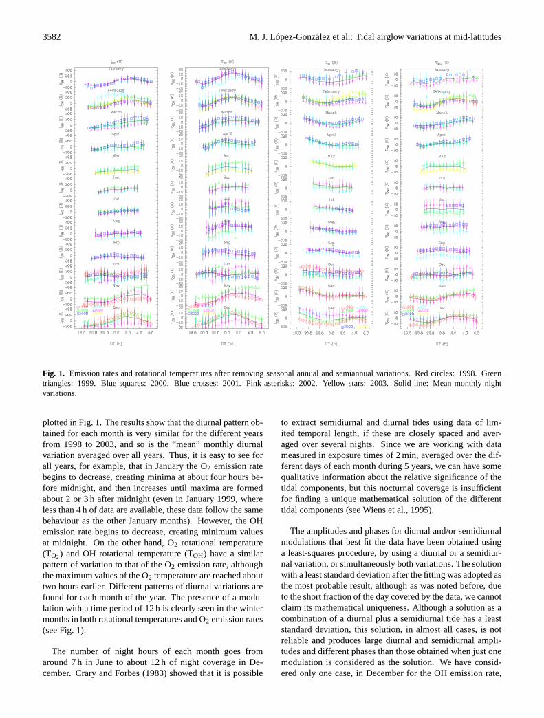
Fig. 1. Emission rates and rotational temperatures after removing seasonal annual and semiannual variations. Red circles: 1998. Greentriangles: 1999. Blue squares: 2000. Blue crosses: 2001. Pink asterisks: 2002. Yellow stars: 2003. Solid line: Mean monthly nightvariations.

plotted in Fig. 1. The results show that the diurnal pattern ob-tained for each month is very similar for the different yearsfrom 1998 to 2003, and so is the “mean” monthly diurnalvariation averaged over all years. Thus, it is easy to see forall years, for example, that in January the O2 emission ratebegins to decrease, creating minima at about four hours be-fore midnight, and then increases until maxima are formedabout 2 or 3 h after midnight (even in January 1999, whereless than 4 h of data are available, these data follow the samebehaviour as the other January months). However, the OHemission rate begins to decrease, creating minimum valuesat midnight. On the other hand, O2 rotational temperature(TO2) and OH rotational temperature (TOH) have a similarpattern of variation to that of the O2 emission rate, althoughthe maximum values of the O2 temperature are reached abouttwo hours earlier. Different patterns of diurnal variations arefound for each month of the year. The presence of a modu-lation with a time period of 12 h is clearly seen in the wintermonths in both rotational temperatures and O2 emission rates(see Fig. 1).

The number of night hours of each month goes fromaround 7 h in June to about 12 h of night coverage in De-cember.Crary and Forbes(1983) showed that it is possible

to extract semidiurnal and diurnal tides using data of lim-ited temporal length, if these are closely spaced and aver-aged over several nights. Since we are working with datameasured in exposure times of 2 min, averaged over the dif-ferent days of each month during 5 years, we can have somequalitative information about the relative significance of thetidal components, but this nocturnal coverage is insufficientfor finding a unique mathematical solution of the differenttidal components (seeWiens et al., 1995).

The amplitudes and phases for diurnal and/or semidiurnalmodulations that best fit the data have been obtained usinga least-squares procedure, by using a diurnal or a semidiur-nal variation, or simultaneously both variations. The solutionwith a least standard deviation after the fitting was adopted asthe most probable result, although as was noted before, dueto the short fraction of the day covered by the data, we cannotclaim its mathematical uniqueness. Although a solution as acombination of a diurnal plus a semidiurnal tide has a leaststandard deviation, this solution, in almost all cases, is notreliable and produces large diurnal and semidiurnal ampli-tudes and different phases than those obtained when just onemodulation is considered as the solution. We have consid-ered only one case, in December for the OH emission rate,


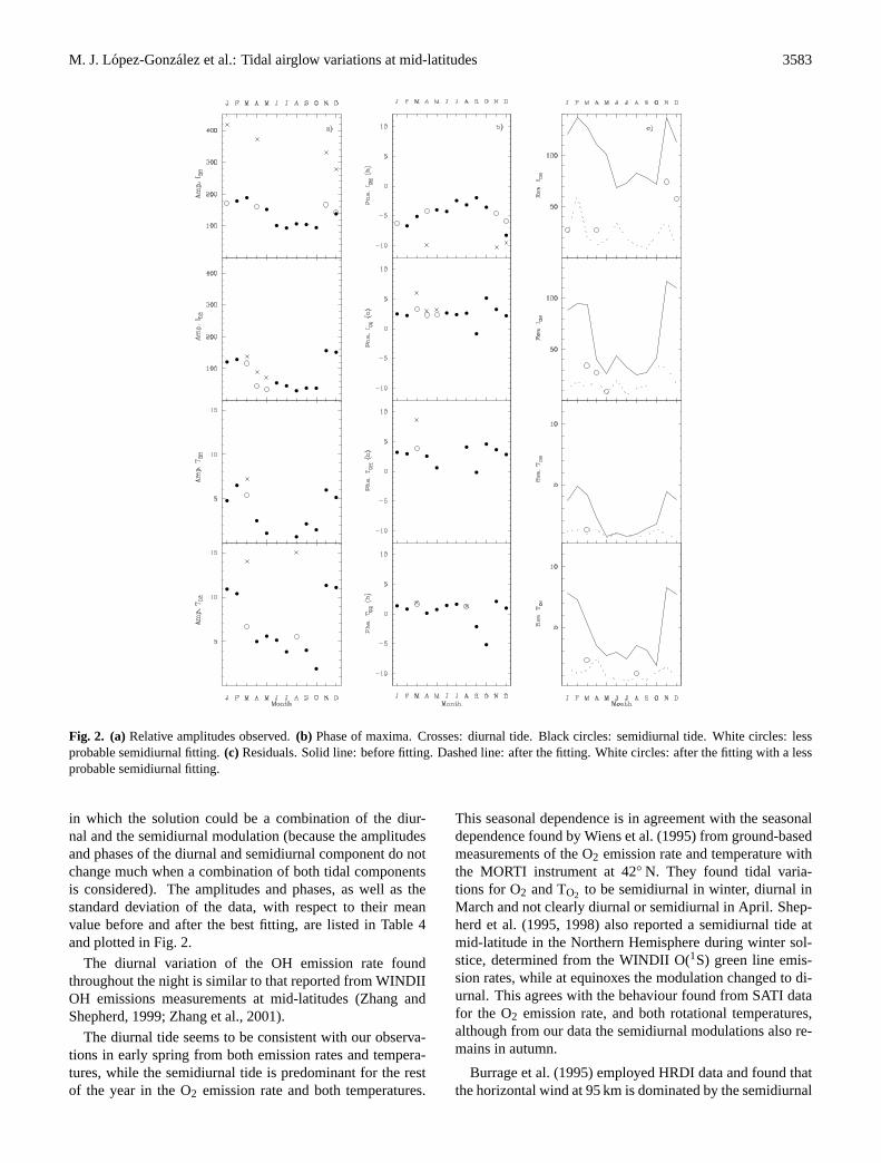
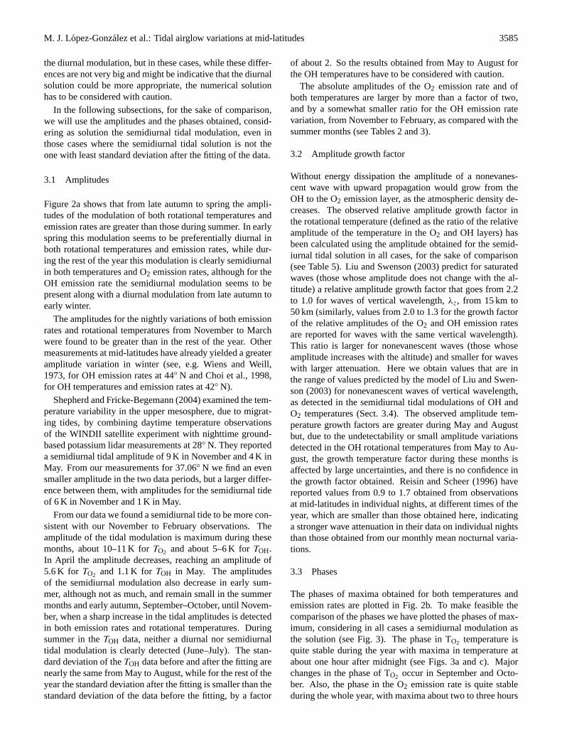
Fig. 2. (a)Relative amplitudes observed.(b) Phase of maxima. Crosses: diurnal tide. Black circles: semidiurnal tide. White circles: lessprobable semidiurnal fitting.(c) Residuals. Solid line: before fitting. Dashed line: after the fitting. White circles: after the fitting with a lessprobable semidiurnal fitting.

in which the solution could be a combination of the diur-nal and the semidiurnal modulation (because the amplitudesand phases of the diurnal and semidiurnal component do notchange much when a combination of both tidal componentsis considered). The amplitudes and phases, as well as thestandard deviation of the data, with respect to their meanvalue before and after the best fitting, are listed in Table 4and plotted in Fig. 2.

The diurnal variation of the OH emission rate foundthroughout the night is similar to that reported from WINDIIOH emissions measurements at mid-latitudes (Zhang andShepherd, 1999; Zhang et al., 2001).

The diurnal tide seems to be consistent with our observa-tions in early spring from both emission rates and tempera-tures, while the semidiurnal tide is predominant for the restof the year in the O2 emission rate and both temperatures.

This seasonal dependence is in agreement with the seasonaldependence found byWiens et al.(1995) from ground-basedmeasurements of the O2 emission rate and temperature withthe MORTI instrument at 42◦ N. They found tidal varia-tions for O2 and TO2 to be semidiurnal in winter, diurnal inMarch and not clearly diurnal or semidiurnal in April.Shep-herd et al.(1995, 1998) also reported a semidiurnal tide atmid-latitude in the Northern Hemisphere during winter sol-stice, determined from the WINDII O(1S) green line emis-sion rates, while at equinoxes the modulation changed to di-urnal. This agrees with the behaviour found from SATI datafor the O2 emission rate, and both rotational temperatures,although from our data the semidiurnal modulations also re-mains in autumn.

Burrage et al.(1995) employed HRDI data and found thatthe horizontal wind at 95 km is dominated by the semidiurnal


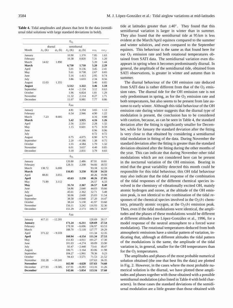
Table 4. Tidal amplitudes and phases that best fit the data (semidi-urnal tidal solutions with large standard deviations in bold).

TO2

diurnal semidiurnalMonth A1 (K) φ1 (h) A2 (K) φ2 (h) resi resf

January 10.90 1.370 7.85 1.63February 10.38 0.820 7.31 1.20March 14.02 1.890 5.20 1.44March 6.730 1.710 5.20 2.29April 5.01 0.136 3.45 2.41May 5.61 0.738 2.67 0.83June 5.16 1.413 2.95 0.74July 3.86 1.633 2.34 0.56August 15.03 1.355 3.46 0.85August 5.512 1.322 3.46 1.18September 4.04 −2.134 3.12 0.63October 1.96 6.824 1.81 1.29November 11.32 2.114 8.27 1.71December 11.07 0.981 7.77 0.86

TOH

January 4.81 3.194 3.65 1.12February 6.54 2.946 4.90 1.22March 7.23 8.685 4.16 0.88March 5.42 3.925 4.16 1.26April 2.56 2.551 2.28 1.32May 1.15 0.601 0.75 0.59June 0.96 0.96July 0.72 0.72August 0.75 4.075 0.90 0.73September 2.20 −0.186 1.38 0.75October 1.55 4.584 1.70 1.32November 6.01 3.637 4.40 0.85December 5.18 2.831 3.79 0.65

IO2

January 120.80 2.486 87.91 10.81February 128.31 2.208 94.66 18.55March 138.72 6.000 93.18 12.33March 116.85 3.258 93.18 34.33April 88.81 3.055 40.26 19.98April 43.63 2.258 40.26 27.05May 71.89 3.112 26.57 6.33May 35.74 2.367 26.57 8.40June 54.86 2.640 44.03 19.66July 45.61 2.362 32.71 5.48August 30.06 2.600 25.03 11.54September 38.58 −0.848 27.20 14.47October 38.24 5.130 41.97 33.60November 156.11 3.242 116.93 32.36December 151.29 2.173 109.72 16.97

IOH

January 417.11 −12.201 120.69 20.17January 171.24 −6.211 120.69 27.54February 178.30 −6.696 136.97 63.53March 188.70 −5.118 127.77 20.29April 371.22 −9.559 111.34 12.35April 160.94 −4.154 111.34 27.53May 151.83 −4.011 101.27 17.30June 101.03 −4.274 69.09 33.90July 93.47 −2.448 73.41 18.47August 106.71 −3.164 83.06 11.98September 104.27 −1.961 78.36 9.23October 94.43 −3.571 71.53 21.52November 332.28 −10.241 137.63 36.35November 165.98 −4.628 137.63 74.60December 277.93 −9.585 137.91 −8.283 113.16 11.26December 142.66 −5.854 113.16 57.60

tide at latitudes greater than±40◦. They found that thissemidiurnal variation is larger in winter than in summer.They also found that the semidiurnal tide at 95 km is lessevident at the March/April equinox compared to the summerand winter solstices, and even compared to the Septemberequinox. This behaviour is the same as that found here forour O2 emission rate and both rotational temperatures ob-tained from SATI data. The semidiurnal variation even dis-appears in spring when it becomes predominantly diurnal. Ingeneral, the amplitude of the semidiurnal tide, obtained fromSATI observations, is greater in winter and autumn than insummer.

The diurnal behaviour of the OH emission rate deducedfrom SATI data is rather different from that of the O2 emis-sion rates. The diurnal tide for the OH emission rate is notonly predominant in spring, as for the O2 emission rate andboth temperatures, but also seems to be present from late au-tumn to early winter. Although this tidal behaviour of the OHemission rate during winter suggests that the diurnal type ofmodulation is present, the conclusion has to be consideredwith caution, because, as can be seen in Table 4, the standarddeviation after the fitting is significantly smaller for Decem-ber, while for January the standard deviation after the fittingis very close to that obtained by considering a semidiurnaltidal modulation in fitting of the data. During November thestandard deviation after the fitting is greater than the standarddeviation obtained after the fitting during the other months ofthe year. This can indicate that during November other tidalmodulations which are not considered here can be presentin the nocturnal variation of the OH emission. Bearing inmind that the great variability detected this month could beresponsible for this tidal behaviour, this OH tidal behaviourmay also indicate that the tidal response of the combinationof the tidal responses of the different chemical species in-volved in the chemistry of vibrationally excited OH, mainlyatomic hydrogen and ozone, at the altitude of the OH emis-sion peak, is not identical to the combination of the tidal re-sponses of the chemical species involved in the O2(b) chem-istry, primarily atomic oxygen, at the O2(b) emission peak.Then, even if the tidal modulations were identical, the ampli-tudes and the phases of these modulations would be differentat different altitudes (seeLopez-Gonzalez et al., 1996, for amodel response of the neutral atmosphere to a forced wavemodulation). The rotational temperatures deduced from bothatmospheric emissions have a similar pattern of variation, in-dicating that, although at different altitudes the tidal patternof the modulations is the same, the amplitude of the tidalvariation is, in general, smaller for the OH temperatures thanfor the O2 temperatures.

The amplitudes and phases of the most probable numericalsolution obtained (the one that best fits the data) are plottedin Fig. 2. However, in the cases where the most probable nu-merical solution is the diurnal, we have plotted these ampli-tudes and phases together with those obtained with a possiblesemidiurnal modulation (also listed in Table 4 with bold char-acters). In these cases the standard deviations of the semidi-urnal modulation are a little greater than those obtained with


the diurnal modulation, but in these cases, while these differ-ences are not very big and might be indicative that the diurnalsolution could be more appropriate, the numerical solutionhas to be considered with caution.

In the following subsections, for the sake of comparison,we will use the amplitudes and the phases obtained, consid-ering as solution the semidiurnal tidal modulation, even inthose cases where the semidiurnal tidal solution is not theone with least standard deviation after the fitting of the data.

3.1 Amplitudes

Figure 2a shows that from late autumn to spring the ampli-tudes of the modulation of both rotational temperatures andemission rates are greater than those during summer. In earlyspring this modulation seems to be preferentially diurnal inboth rotational temperatures and emission rates, while dur-ing the rest of the year this modulation is clearly semidiurnalin both temperatures and O2 emission rates, although for theOH emission rate the semidiurnal modulation seems to bepresent along with a diurnal modulation from late autumn toearly winter.

The amplitudes for the nightly variations of both emissionrates and rotational temperatures from November to Marchwere found to be greater than in the rest of the year. Othermeasurements at mid-latitudes have already yielded a greateramplitude variation in winter (see, e.g.Wiens and Weill,1973, for OH emission rates at 44◦ N andChoi et al., 1998,for OH temperatures and emission rates at 42◦ N).

Shepherd and Fricke-Begemann(2004) examined the tem-perature variability in the upper mesosphere, due to migrat-ing tides, by combining daytime temperature observationsof the WINDII satellite experiment with nighttime ground-based potassium lidar measurements at 28◦ N. They reporteda semidiurnal tidal amplitude of 9 K in November and 4 K inMay. From our measurements for 37.06◦ N we find an evensmaller amplitude in the two data periods, but a larger differ-ence between them, with amplitudes for the semidiurnal tideof 6 K in November and 1 K in May.

From our data we found a semidiurnal tide to be more con-sistent with our November to February observations. Theamplitude of the tidal modulation is maximum during thesemonths, about 10–11 K forTO2 and about 5–6 K forTOH.In April the amplitude decreases, reaching an amplitude of5.6 K for TO2 and 1.1 K forTOH in May. The amplitudesof the semidiurnal modulation also decrease in early sum-mer, although not as much, and remain small in the summermonths and early autumn, September–October, until Novem-ber, when a sharp increase in the tidal amplitudes is detectedin both emission rates and rotational temperatures. Duringsummer in theTOH data, neither a diurnal nor semidiurnaltidal modulation is clearly detected (June–July). The stan-dard deviation of theTOH data before and after the fitting arenearly the same from May to August, while for the rest of theyear the standard deviation after the fitting is smaller than thestandard deviation of the data before the fitting, by a factor

of about 2. So the results obtained from May to August forthe OH temperatures have to be considered with caution.

The absolute amplitudes of the O2 emission rate and ofboth temperatures are larger by more than a factor of two,and by a somewhat smaller ratio for the OH emission ratevariation, from November to February, as compared with thesummer months (see Tables 2 and 3).

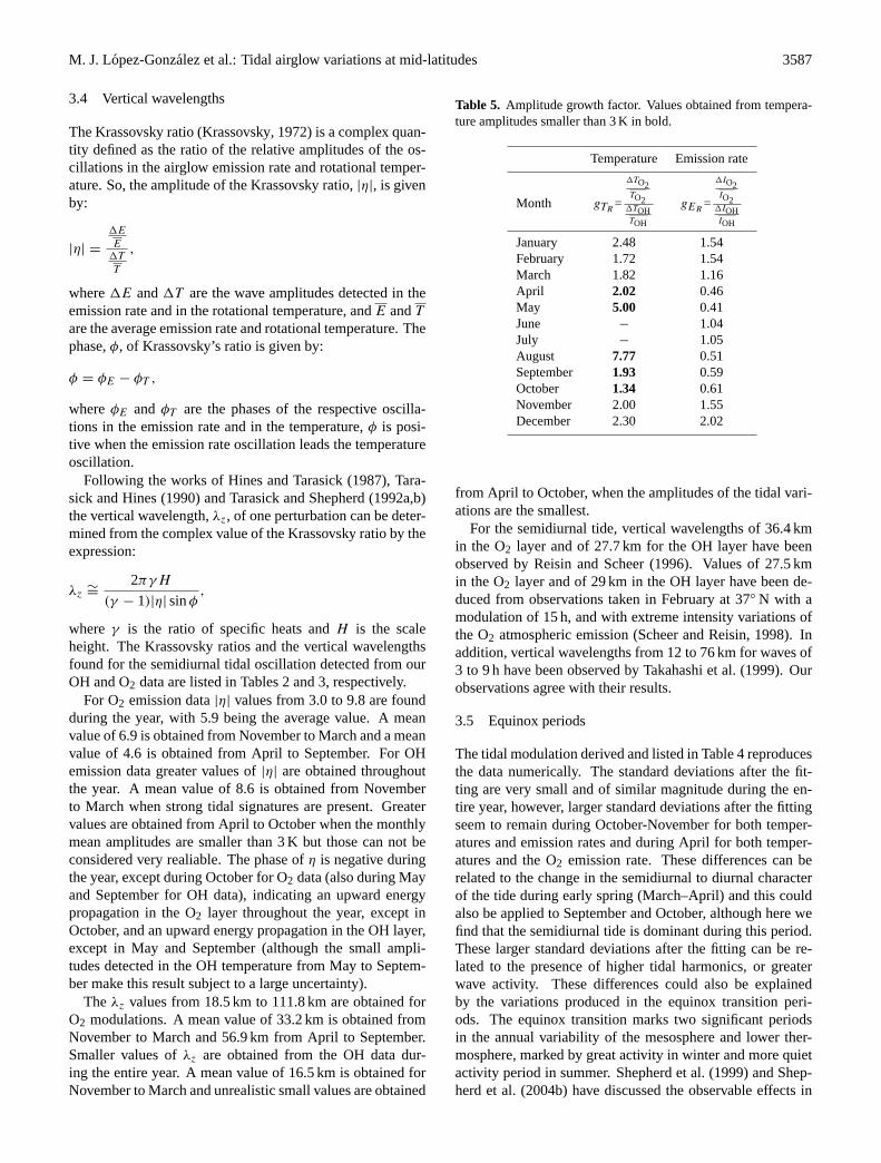
3.2 Amplitude growth factor

Without energy dissipation the amplitude of a nonevanes-cent wave with upward propagation would grow from theOH to the O2 emission layer, as the atmospheric density de-creases. The observed relative amplitude growth factor inthe rotational temperature (defined as the ratio of the relativeamplitude of the temperature in the O2 and OH layers) hasbeen calculated using the amplitude obtained for the semid-iurnal tidal solution in all cases, for the sake of comparison(see Table 5).Liu and Swenson(2003) predict for saturatedwaves (those whose amplitude does not change with the al-titude) a relative amplitude growth factor that goes from 2.2to 1.0 for waves of vertical wavelength,λz, from 15 km to50 km (similarly, values from 2.0 to 1.3 for the growth factorof the relative amplitudes of the O2 and OH emission ratesare reported for waves with the same vertical wavelength).This ratio is larger for nonevanescent waves (those whoseamplitude increases with the altitude) and smaller for waveswith larger attenuation. Here we obtain values that are inthe range of values predicted by the model ofLiu and Swen-son(2003) for nonevanescent waves of vertical wavelength,as detected in the semidiurnal tidal modulations of OH andO2 temperatures (Sect. 3.4). The observed amplitude tem-perature growth factors are greater during May and Augustbut, due to the undetectability or small amplitude variationsdetected in the OH rotational temperatures from May to Au-gust, the growth temperature factor during these months isaffected by large uncertainties, and there is no confidence inthe growth factor obtained.Reisin and Scheer(1996) havereported values from 0.9 to 1.7 obtained from observationsat mid-latitudes in individual nights, at different times of theyear, which are smaller than those obtained here, indicatinga stronger wave attenuation in their data on individual nightsthan those obtained from our monthly mean nocturnal varia-tions.

3.3 Phases

The phases of maxima obtained for both temperatures andemission rates are plotted in Fig. 2b. To make feasible thecomparison of the phases we have plotted the phases of max-imum, considering in all cases a semidiurnal modulation asthe solution (see Fig. 3). The phase in TO2 temperature isquite stable during the year with maxima in temperature atabout one hour after midnight (see Figs. 3a and c). Majorchanges in the phase of TO2 occur in September and Octo-ber. Also, the phase in the O2 emission rate is quite stableduring the whole year, with maxima about two to three hours


Fig. 3. Phases of maximum.(a) TO2 and IO2. (b) TOH andIOH.(c) TO2 andTOH. (d) IOH andIO2. White circle (solid line):TO2.White star (solid line):IO2. Black circle (dashed line):TOH. Blackstar (dashed line):IOH.

after midnight. There are exceptions to this stable phase be-haviour, as in the O2 temperature, for the months of Septem-ber and October. It can be seen that the maxima in the O2emission rates occur about one or two hours later than thosein TO2. So, O2 temperatures lead the O2 emission rates. Thispattern is maintained for almost the whole year.

The time of the OH temperature maximum is also rela-tively stable during the year, with a maximum in OH rota-tional temperature at about a mean value of 4 h after midnight(see Figs. 3b and c). Again, large oscillations seem to be ob-tained at the times of the OH temperature maximum duringSeptember.

From Fig. 3c it is easy to see that the time of the OHtemperature maximum is about 2 h later than the time of themaximum in O2 temperature, with the exception of May andOctober, where the times of maximum OH temperature leadthose of the O2 temperature (see Fig. 3c). Thus, with thoseexceptions, and bearing in mind that the fitting of OH temper-atures is difficult to detect from May to August (see Fig. 2band Table 4), O2 rotational temperatures lead OH tempera-tures for almost the entire year.

Figures 3b and d show that the maximum in the OH emis-sion rate is always later than midnight. The maximum isabout 6 h later than midnight from December to February (or6 h before midnight). This means that OH emission ratesreach minimum values close to midnight from December toFebruary. From March to September the maximum valuesof the OH emission rates move toward later times, from 7 hlater than midnight in March to 10 h later than midnight inSeptember (or from 5 to 2 h before midnight, respectively).Then maximum values of OH emission rates move to ear-lier times in the night, as in winter months, from October toNovember.

The comparison of the times of maximum of the OH emis-sion rates and temperatures shows that the OH emission ratesreach a maximum about 3–4 h later than the maximum in OHtemperatures from August to March, except in September,where the OH emission rate is maximum two hour before thatof the OH temperature. During April and May the differencebetween the time of maximum OH emission rate and tem-perature increases, although it is during these months whenit is difficult to find a semidiurnal modulation in OH temper-atures.

The derived semidiurnal parameters from the SATI OHand O2 temperature data have been compared with the semid-iurnal parameters predicted by the Global Scale Wave Model(GSWM) (Hagan et al., 1999). The derived SATI phases ofthe temperature semidiurnal tide agree very well with thosepredicted by the GSWM at the respective heights. The OHsemidiurnal phases of about 3–4 h local time are in excellentagreement with the GSWM phases predicted for the semid-iurnal tide of about 15–16 h (or 3–4 h) solar local time, at86.3 km height and 36 N latitude. Similarly, the O2 semid-iurnal tide phases are obtained at about 1–2 h local time, inagreement with the GSWM semidiurnal tide phases of 14–15 h (or 2–3 h) solar local time at 94.6 km height and 36 N.Further, the change in the OH phase derived from SATI forthe month of September is in very good agreement with theGSWM model, while the change in the phase of the O2semidiurnal tide derived during September-October is pre-dicted earlier in the model, from July to September. Al-though our derived SATI temperature semidiurnal tide am-plitudes are somewhat larger than those predicted by theGSWM model, in general a good agreement is obtained be-tween the SATI derived semidiurnal tide parameters and theparameters predicted by the GSWM model.


3.4 Vertical wavelengths

The Krassovsky ratio (Krassovsky, 1972) is a complex quan-tity defined as the ratio of the relative amplitudes of the os-cillations in the airglow emission rate and rotational temper-ature. So, the amplitude of the Krassovsky ratio,|η|, is givenby:

|η| =

1E

E1T

T

,

where1E and1T are the wave amplitudes detected in theemission rate and in the rotational temperature, andE andT

are the average emission rate and rotational temperature. Thephase,φ, of Krassovsky’s ratio is given by:

φ = φE − φT ,

whereφE and φT are the phases of the respective oscilla-tions in the emission rate and in the temperature,φ is posi-tive when the emission rate oscillation leads the temperatureoscillation.

Following the works ofHines and Tarasick(1987), Tara-sick and Hines(1990) andTarasick and Shepherd(1992a,b)the vertical wavelength,λz, of one perturbation can be deter-mined from the complex value of the Krassovsky ratio by theexpression:

λz∼=

2πγH

(γ − 1)|η| sinφ,

where γ is the ratio of specific heats andH is the scaleheight. The Krassovsky ratios and the vertical wavelengthsfound for the semidiurnal tidal oscillation detected from ourOH and O2 data are listed in Tables 2 and 3, respectively.

For O2 emission data|η| values from 3.0 to 9.8 are foundduring the year, with 5.9 being the average value. A meanvalue of 6.9 is obtained from November to March and a meanvalue of 4.6 is obtained from April to September. For OHemission data greater values of|η| are obtained throughoutthe year. A mean value of 8.6 is obtained from Novemberto March when strong tidal signatures are present. Greatervalues are obtained from April to October when the monthlymean amplitudes are smaller than 3 K but those can not beconsidered very realiable. The phase ofη is negative duringthe year, except during October for O2 data (also during Mayand September for OH data), indicating an upward energypropagation in the O2 layer throughout the year, except inOctober, and an upward energy propagation in the OH layer,except in May and September (although the small ampli-tudes detected in the OH temperature from May to Septem-ber make this result subject to a large uncertainty).

Theλz values from 18.5 km to 111.8 km are obtained forO2 modulations. A mean value of 33.2 km is obtained fromNovember to March and 56.9 km from April to September.Smaller values ofλz are obtained from the OH data dur-ing the entire year. A mean value of 16.5 km is obtained forNovember to March and unrealistic small values are obtained

Table 5. Amplitude growth factor. Values obtained from tempera-ture amplitudes smaller than 3 K in bold.

Temperature Emission rate

Month gTR=

1TO2TO2

1TOHTOH

gER=

1IO2IO2

1IOHIOH

January 2.48 1.54February 1.72 1.54March 1.82 1.16April 2.02 0.46May 5.00 0.41June − 1.04July − 1.05August 7.77 0.51September 1.93 0.59October 1.34 0.61November 2.00 1.55December 2.30 2.02

from April to October, when the amplitudes of the tidal vari-ations are the smallest.

For the semidiurnal tide, vertical wavelengths of 36.4 kmin the O2 layer and of 27.7 km for the OH layer have beenobserved byReisin and Scheer(1996). Values of 27.5 kmin the O2 layer and of 29 km in the OH layer have been de-duced from observations taken in February at 37◦ N with amodulation of 15 h, and with extreme intensity variations ofthe O2 atmospheric emission (Scheer and Reisin, 1998). Inaddition, vertical wavelengths from 12 to 76 km for waves of3 to 9 h have been observed byTakahashi et al.(1999). Ourobservations agree with their results.

3.5 Equinox periods

The tidal modulation derived and listed in Table 4 reproducesthe data numerically. The standard deviations after the fit-ting are very small and of similar magnitude during the en-tire year, however, larger standard deviations after the fittingseem to remain during October-November for both temper-atures and emission rates and during April for both temper-atures and the O2 emission rate. These differences can berelated to the change in the semidiurnal to diurnal characterof the tide during early spring (March–April) and this couldalso be applied to September and October, although here wefind that the semidiurnal tide is dominant during this period.These larger standard deviations after the fitting can be re-lated to the presence of higher tidal harmonics, or greaterwave activity. These differences could also be explainedby the variations produced in the equinox transition peri-ods. The equinox transition marks two significant periodsin the annual variability of the mesosphere and lower ther-mosphere, marked by great activity in winter and more quietactivity period in summer.Shepherd et al.(1999) andShep-herd et al.(2004b) have discussed the observable effects in


the oxygen airglow during the spring and autumn transitionswhileShepherd et al.(2002) andShepherd et al.(2004a) havediscussed the observable effects during the spring and au-tumn transition in the atmospheric temperature.

From the present work, the equinox periods could be char-acterized by:

1. Great changes in the phases of the tidal variations.These changes in the phases of the tidal activity dur-ing the months of September-October could be an in-dication of these transition periods (during March thephases of tidal activity show some changes but not asmarked as during the September-October months).

2. During March-April and during September-October asmall growth factor is detected for both temperatureamplitudes and emission rate amplitudes, indicating agreater degree of dissipation than during the rest of theyear (see Table 5).

3. The fact that large standard deviations after the fittingare obtained for October–November, in both temper-atures and emission rates, and somewhat larger stan-dard deviations after the fitting are present for April, inboth temperatures and O2 emission rates, than duringthe rest of the year, can be connected to the presence ofhigher tidal harmonic and wave activity and also withthe changes that are produced due to the equinox transi-tions during these periods.

4 Conclusions

The monthly mean diurnal variations for temperatures andemission rates, deduced from the OH(6-2) Meinel and O2(0-1) atmospheric bands at a latitude of 37.06◦ N, from SATIoperation in 1998 to 2003, have been presented. A clear dailymodulation is found in temperatures and emission rates:

– The modulation is predominantly semidiurnal in bothtemperatures and emission rates throughout the year.

– During spring the semidiurnal variation changes to a di-urnal type, in both temperature and emission rates.

– During late autumn and early winter OH emission ratesshow both diurnal and semidiurnal modulations.

From summer to late autumn the amplitudes of the diurnalvariation decrease by more than a factor of two comparedwith those in winter and spring.

Mean vertical wavelengths for the semidiurnal modulationof 33.2 km in the O2 layer and of 16.5 km for the OH layerare obtained from November to March with our data.

A clear upward energy propagation is observed duringmost of the year, with some indication of possible downwardenergy propagation close to the equinoxes.

Both emission rates and rotational temperatures present asimilar pattern of diurnal variation throughout the year, yield-ing maximum values some time after midnight.

It is clear that, in general, TO2 leads the O2 emission rates,that O2 rotational temperatures also lead the OH rotationaltemperatures and that TOH leads the OH emission rates. Bothemission rates have phase shifts from about 3 h to 7 h (−5 h)for the entire year, with the O2 emission rate leading the OHemission rate, expect in July, August and September, whenthe OH emission rate leads the O2 emission rate.

Acknowledgement.This research was partially supported by the Di-reccion General de Investigacion (DGI) under projects AYA2000-1559 and AYA2003-04651, the Comision Interministerial de Cien-cia y Tecnologıa under projects REN2001-3249 and ESP2004–01556, the Junta de Andalucıa, NATO under a Collaborative Link-age Grants 977354 and 979480 and INTAS under the researchproject 03-51-6425. We very gratefully acknowledge the staff ofSierra Nevada Observatory for their help and assistance with theSATI instrument. We wish to thank the referee for useful commentsand suggestions.

Topical Editor U. P. Hoppe thanks a referee for his/her help inevaluating this paper.

References

Abreu, V. J. and Yee, J. H.: Diurnal and seasonal variation of thenighttime OH(8-3) emission at low latitudes, J. Geophys. Res.,94, 11 949–11 957, 1989.

Burrage, M. D., Arvin, N., Skinner, W. R., and Hays, P. B.: Obser-vations of the O2 atmospheric band nightglow by the High Res-olution Doppler Imager, J. Geophys. Res., 99, 15 017–15 023,1994.

Burrage, M. D., Wu, D. L., Skinner, W. R., Ortland, D. A., andHays, P. B.: Latitude and seasonal dependence of the semidiurnaltide observed by the high-resolution Doppler imager, J. Geophys.Res., 100, 11 313–11 321, 1995.

Crary, J. D. and Forbes, J. M.: On the extraction of tidal informationfrom measurements covering a fraction of a day, Geophys. Res.Lett., 10, 580–582, 1983.

Chapman, S. and Lindzen, R. S.: Atmospheric tides: thermal andgravitational, Gordon and Breach, New York, 1–23, 1970.

Choi, G. H., Monson, I. K., Wickwar, V. B., and Rees, D.: Sea-sonal and diurnal variations of wind and temperature near themesopause from Fabry-Perot interferometer observations of OHMeinel emissions, Adv. Space Res., 21, 847–850, 1998.

Forbes, J. M., Portnyagin, Yu. I., Skinner, W., Vincent, R. A.,Solovjova, T., Merzlyakov, E., Nakamura, T., and Palo, S.: Cli-matological lower thermosphere winds as seen by ground-basedand space-based instruments, Ann. Geophys., 22, 1931–1945,2004,SRef-ID: 1432-0576/ag/2004-22-1931.

Hagan, M. E., Burrage, M. D., Forbes, J. M., Hackney, J., Randel,W. J., and Zhang, X.: GSWM-98: Results for migrating solartides, J. Geophys. Res., 104, 6813–6828, 1999.

Hines, C. O. and Tarasick, D. W.: On the detection and utilizationof gravity waves in airglow studies, Planet. Space Sci., 35, 851–866, 1987.

Jacobi, Ch., Portnyagin, Yu. I., Solovjova, T. V., Hoffmann, P.,Singer, W., Fahrutdinova, A. N., Ishmuratov, R. A., Beard, A.G., Mitchell, N. J., Muller, H. G., Schminder, R., Kurschner, D.,Manson, A. H., and Meek, C. E.: Climatology of the semidiur-nal tide at 52–56 N from ground-based radar wind measurements1985–1995, J. Atmos. Solar-Terr. Phys., 61, 975–991, 1999.

http://direct.sref.org/1432-0576/ag/2004-22-1931


Krassovsky, V. I.: Infrasonic variations of OH emission in the upperatmosphere, Ann. Geophys., 28, 739–746, 1972.

Liu, A. Z. and Swenson, G. R.: A modeling study of O2 and OHairglow perturbations induced by atmospheric gravity waves, J.Geophys. Res., 108(D4), 4151, doi:10.1029/2002JD2474, 2003.

Lopez-Gonzalez, M. J., Murtagh, D. P., Espy, P. J., Lopez-Moreno,J. J., Rodrigo, R., and Witt, G.: A model study of the temporalbehaviour of the emission intensity and rotational temperature ofthe OH Meinel bands for high-latitude summer conditions, Ann.Geophys., 14, 59–67, 1996,SRef-ID: 1432-0576/ag/1996-14-59.

Lopez-Gonzalez, M. J., Rodrıguez, E., Wiens, R. H., Shepherd, G.G., Sargoytchev, S., Brown, S., Shepherd, M. G., Aushev, V.M., Lopez-Moreno, J. J., Rodrigo, R., and Cho, Y.-M.: Seasonalvariations of O2 Atmospheric and OH(6-2) airglow and temper-ature at mid-latitudes from SATI observations, Ann. Geophys.,22, 819–828, 2004,SRef-ID: 1432-0576/ag/2004-22-819.

Manson, A. H., Meek, C. E., Chshyolkova, T., Avery, S. K.,Thorsen, D., MacDougall, J. W., Hocking, W., Murayama, Y.,Igarashi, K., Namboothiri, S. P., and Kishore, P.: Longitudinaland latitudinal variations in dynamic characteristics of the MLT(70–95 km): a study involving the CUJO network, Ann. Geo-phys., 22, 347–365, 2004,SRef-ID: 1432-0576/ag/2004-22-347.

Pancheva, D., Mukhtarov, P., Mitchell, N. J., Beard, A. G., andMuller, H. G.: A comparative study of winds and tidal variabilityin the mesosphere/lower-thermosphere region over Bulgaria andthe UK, Ann. Geophys., 18, 1304–1315, 2000,SRef-ID: 1432-0576/ag/2000-18-1304.

Pancheva, D., Merzlyakov, E., Mitchell, N. J., Portnyagin, Yu.,Manson, A. H., Jacobi, Ch., Meek, C. E., Luo, Y., Clark, R. R.,Hocking, W. K., MacDougall, J., Muller, H. G., Kurschner, D.,Jones, G. O. L., Vincent, R. A., Reid, I. M., Singer, W., Igarashi,K., Fraser, G. I., Fahrutdinova, A. N., Stepanov, A. M., Poole,L. M. G., Malinga, S. B., Kashcheyev, B. L., and Oleynikov, A.N.: Global-scale tidal variability during the PSMOS campaign ofJune–August 1999: interaction with planetary waves, J. Atmos.Solar-Terr. Phys., 64, 1865–1896, 2002.

Pendleton Jr., W. R. and Taylor, M. J.: The impact of L-uncouplingon Einstein coefficients for the OH Meinel (6,2) band: implica-tions for Q-branch rotational temperatures, J. Atmos. Solar-Terr.Phys., 64, 971–983, 2002.

Petitdidier, M. and Teitelbaum, H.: Lower thermosphere emissionsand tides, Planet. Space Sci., 25, 711–721, 1977.

Portnyagin, Y. I., Solovjova, T. V., Makarov, N. A., Merzlyakov,E. G., Manson, A. H., Meek, C. E., Hocking, W., Mitchell, N.,Pancheva, D., Hoffmann, P., Singer, W., Murayama, Y., Igarashi,K., Forbes, J. M., Palo, S., Hall, C., and Nozawa, S.: Monthlymean climatology of the prevailing winds and tides in the Arc-tic mesosphere/lower thermosphere, Ann. Geophys., 22, 3395–3410, 2004,SRef-ID: 1432-0576/ag/2004-22-3395.

Reisin, E. R. and Scheer, J.: Characteristics of atmospheric waves inthe tidal period range derived from zenith observations of O2(0-1) Atmospheric and OH(6-2) airglow at lower midlatitudes, J.Geophys. Res., 101, 21 223–21 232, 1996.

Riggin, D. M., Meyer, C. K., Fritts, D. C., Jarvis, M. J., Murayama,Y., Singer, W., Vincent, R. A., and Murphy, D. J.: MF radarobservations of seasonal variability of semidiurnal motions in themesosphere at high northern and southern latitudes, J. Atmos.Solar-Terr. Phys., 65, 483–493, 2003.

Sargoytchev, S., Brown, S., Solheim, B. H., Cho, Y.-M., Shepherd,G. G., and Lopez-Gonzalez, M. J.: Spectral airglow temperatureimager (SATI) – a ground based instrument for temperature mon-itoring of the mesosphere region, Appl. Opt., 43, 5712–5721,2004.

Scheer, J. and Reisin, E. R.: Rotational temperatures for OH andO2 airglow bands measured simultaneously from El Leoncito(31◦48′ S), J. Atmos. Terr. Phys., 52, 47–57, 1990.

Scheer, J. and Reisin, E. R.: Extreme intensity variations of O2bairglow induced by tidal oscillations, Adv. Space Res., 21, 827–830, 1998.

Shepherd, M. G. and Fricke-Begemann, C.: Study of the tidal vari-ations in mesospheric temperature at low and mid latitudes fromWINDII and potassium lidar observations, Ann. Geophys., 22,1513–1528, 2004,SRef-ID: 1432-0576/ag/2004-22-1513.

Shepherd, G. G., McLandress, C., and Solheim, B. H.: Tidal in-fluence on O(1S) airglow emission rate distributions at the ge-ographic equator as observed by WINDII, Geophys. Res. Lett.,22, 275–278, 1995.

Shepherd, G. G., Roble, R. G., Zhang, S. P., McLandress, C., andWiens, R. H.: Tidal influences on midlatitude airglow: Compari-son of satellite and ground-based observations with TIME-GCMpredictions, J. Geophys. Res., 103, 14 741–14 751, 1998.

Shepherd, G. G., Stegman, J., Espy, P., McLandress, C., Thuillier,G., and Wiens, R. H.: Springtime transition in lower thermo-spheric atomic oxygen, J. Geophys. Res., 104, 213–223, 1999.

Shepherd, M. G., Espy, P. J., She, C. Y., Hocking, W., Keckhut,P., Gavrilyeva, G., Shepherd, G. G., and Naujokat, B.: Spring-time transition in upper mesospheric temperature in the NorthernHemisphere, J. Atmos. Solar-Terr. Phys., 64, 1183–1199, 2002.

Shepherd, M. G., Rochon, Y. I., Offermann, D., Donner, M., andEspy, P. J.: Longitudinal variability of mesospheric temperaturesduring equinox at middle and high latitudes, J. Atmos. Solar-Terr.Phys., 66, 463–479, 2004a.

Shepherd, G. G., Stegman, J., Singer, W., and Roble, R. G.:Equinox transition in wind and airglow observations, J. Atmos.Solar-Terr. Phys., 66, 481–491, 2004b.

Takahashi, H., Sahai, Y., Clemesha, B. R., Batista, P. P., and Teix-eira, N. R.: Diurnal and seasonal variations of the OH (8,3) air-glow band and its correlation with OI 5577, Planet. Space Sci.,25, 541–547, 1977.

Takahashi, H., Gobbi, D., Batista, P. P., Melo, S. M. L., Teixeira,N. R., and Buriti, R. A.: Dynamical influence on the equatorialairglow observed from the South American sector, Adv. SpaceRes., 21, 817–825, 1998.

Takahashi, H., Batista, P. P., Buriti, R. A, Gobbi, D., Nakamura, T.Tsuda, T., and Fukao, S.: Response of the airglow OH emission,temperature and mesopause wind to the atmospheric wave prop-agation over Shigaraki, Japan, Earth Planets Space, 51, 863–875,1999.

Tarasick, D. W. and Hines, C. O.: The observable effects of gravitywaves on airglow emissions, Planet. Space Sci., 38, 1105–1119,1990.

Tarasick, D. W. and Shepherd, G. G.: Effects of gravity waveson complex airglow chemistries. 1 O2(b16+

g ) emission, J. Geo-phys. Res., 97, 3185–3193, 1992a.

Tarasick, D. W. and Shepherd, G. G.: Effects of gravity waves oncomplex airglow chemistries. 2. OH emission, J. Geophys. Res.,97, 3195–3208, 1992b.

Wiens, R. H. and Weill, G.: Diurnal, annual and solar cyclevariations of hydroxyl and sodium nightglow intensities in the








Europe-Africa sector, Planet. Space Sci., 21, 1011–1027, 1973.Wiens, R. H., Zhang, S. P., Peterson, R. N., and Shepherd, G. G.:

MORTI: A Mesopause Oxygen Rotational Temperature Imager,Planet. Space Sci., 39, 1363–1375, 1991.

Wiens, R. H., Zhang, S. P., Peterson, R. N., and Shepherd, G. G.:Tides in emission rate and temperature from O2 nightglow overBear Lake Observatory, Geophys. Res. Lett., 22, 2637–2640,1995.

Wiens, R. H., Moise, A., Brown, S., Sargoytchev, S., Peterson, R.N., Shepherd, G. G., Lopez-Gonzalez, M. J., Lopez-Moreno, J.J., and Rodrigo, R.: SATI: A Spectral Airglow Temperature Im-ager, Adv. Space Res., 19, 677–680, 1997.

Zhang, S. P. and Shepherd, G. G.: The influence of the diurnal tideon the O(1S) and OH emission rates observed by WINDII onUARS, Geophys. Res. Lett., 26, 529–532, 1999.

Zhang, S. P., Shepherd, G. G., and Roble, R. G.: Tidal influenceon the oxygen and hydroxyl nightglows: Wind Imaging Interfer-ometer observations and thermosphere/ionosphere/mesosphereelectrodynamics general circulation model, J. Geophys. Res.,106, 21 381–21 393, 2001.

Documents

Geophysicae Tidal variations of O Atmospheric and OH(6-2