arX

iv:h

ep-t

h/04

1110

1v1

9 N

ov 2

004

Geometry and analysis in non-linear sigma models

Dave Auckly ∗

Department of Mathematics,Kansas State University,

Manhattan, Kansas 66506, USA

Lev Kapitanski †

Department of Mathematics,University of Miami,

Coral Gabels, Florida 33124, USA

J. Martin Speight ‡

School of Mathematics,

University of Leeds,Leeds LS2 9JT, England

February 7, 2008

Abstract

The configuration space of a non-linear sigma model is the space of maps from onemanifold to another. This paper reviews the authors’ work on non-linear sigma modelswith target a homogeneous space. It begins with a description of the components, fun-damental group, and cohomology of such configuration spaces together with the physicalinterpretations of these results. The topological arguments given generalize to Sobolevmaps. The advantages of representing homogeneous space valued maps by flat connec-tions are described, with applications to the homotopy theory of Sobolev maps, andminimization problems for the Skyrme and Faddeev functionals. The paper concludeswith some speculation about the possiblility of using these techniques to define newinvariants of manifolds.

∗The first author was partially supported by NSF grant DMS-0204651.†The second author was partially supported by NSF grant DMS-0436403.‡The third author was partially supported by EPSRC grant GR/R66982/01.

1

1 Introduction

Physicists have used variational principles to describe physical phenomena for a long time. Theclassical trajectories of a system are modeled as the stationary points of an action functional.The quantum behavior of the system may be modeled in one of two frameworks: Lagrangianor Hamiltonian. The Lagrangian framework uses path integrals of an exponential of the actionfunctional. This has proved to be a very powerful tool for physical modeling and mathematicalinspiration. The Hamiltonian point of view is better understood from a mathematical pointof view, but there is still work to be done in this direction [22].

The first case studied via a variational principle is the motion of a point particle on someconfiguration manifold. The static configurations are the critical points of a potential energy,and the classical trajectories are described by a non-linear system of ordinary differential equa-tions. These equations are the Euler-Lagrange equations of the action functional. The secondcase considers fields such as the electro-magnetic field. A field is a function on a manifoldor more generally a section of a vector bundle over the manifold. The classical dynamics ofa field are described by a generally non-linear system of partial differential equations (theU(1) Yang-Mills equations for electro-magnetic fields or SU(2) × U(1) Yang-Mills equationsfor electro-weak fields). These equations are the Euler-Lagrange equations of a certain func-tional. Quantum Field Theory is the quantum version of this second case. Physicists nowhedge their bets by speaking of effective field theories, [26]. By this they acknowledge thatQuantum Field Theories produce very accurate predictions, but are possibly not the correcttheories to describe the universe. They argue that in certain limiting conditions one QuantumField Theory will accurately model physical behavior, in other limiting conditions some otherQuantum Field Theory will provide the accurate model. It is reasonable to expect that undercertain limiting conditions fields will take values close to the critical points of potential energy.In this situation, one would consider the basic objects to be maps from a manifold to somenon-linear space. This is the usual origin of non-linear sigma models.

A non-linear sigma model is a model with a configuration space consisting of maps fromone manifold M representing space to some target manifold, N , [5]. Techniques from thegeometry of manifolds can shed light on the behavior of non-linear sigma models, and itis possible that non-linear sigma models may prove to be useful tools for the study of thegeometry of manifolds.

In this paper, we will discuss some geometric and analytical techniques that have beenuseful in the study of two non-linear sigma models. We will begin with a discussion of thetopology of the relevant configuration spaces in the first section. In the second section, wewill discuss analytical issues related to these models.

2 Topology of configuration spaces

Mathematically, the challenges within the study of non-linear sigma models arise because thetarget is not a linear or convex space. The topology of the target allows one to considerdifferent types of constraint in an optimization problem. These constraints are an integralfeature of the model. For example, it is common to look for a minimizer of a functional in a

2

fixed homotopy class. If the homotopy class is not constrained it may be that a constant mapwill minimize the functional.

There are in fact many different but related configuration spaces that one could consider.We will concentrate on two general types of configuration space: maps into Lie groups andmaps into S2. Let M be a compact, oriented 3-manifold and G be any Lie group. Then thefirst configuration space we consider is the space of continuous maps M → G which send achosen basepoint x0 ∈ M to I ∈ G. This space is denoted by GM . The second configurationspace is (S2)M .

In this section, we will give configuration spaces the compact open topology. In practicesome Sobolev topology depending on the energy functional is probably appropriate. The issueof checking the algebraic topology arguments given for classes of Sobolev maps is interesting.We will address this issue in the next section. We will motivate the study of the algebraictopology of these spaces by the physical interpretation of the non-linear sigma model. Moredetailed physical and geometric interpretations of the topological results in this section maybe found in [4].

2.1 Components of configuration space

The Skyrme model has been considered as a model of several different systems. In one caseit is used to model nucleons: the protons and neutrons in the center of an atom. Space isassumed to be R3 (this is reasonable when we are modeling the nucleus of an atom). Fieldsare taken to be maps into Sp(1) the group of unit quaternions. In order to have finite energy,the gradient of such a map must have finite L2 norm. It is natural, therefore, to impose theboundary condition that the field approach a constant value as |x| → ∞, where x denotesposition in space. We may choose this boundary value to be 1 without loss of generality. Sowe take our configuration space to be Sp(1)S3

. This is the space of base point preserving mapsfrom S3 to Sp(1). We are viewing S3 as the one point compactification of R3, the base point,infinity, is assumed to map to the base point 1. Notice that topologically Sp(1) is S3. Thehomotopy classes of maps from S3 to Sp(1) are classified by an integer degree. The energyminimizer in the degree 0 class is just the constant map, in physicists’ language, the vacuum.

Linearizing the field equations about the vacuum we obtain a wave equation for a fieldtaking values in sp(1) ∼= R3. Travelling wave solutions of this wave equation represent theπ+, π− and π0 mesons which transmit the strong nuclear force between nucleons. Uponquantization, the Fourier coefficients of a general solution of the wave equation become thepion creation and annihilation operators of the theory. The neutron and proton appear in thismodel as the degree 1 minimizers of the energy functional. More precisely, they are the lowestenergy quantum states built on top of a degree 1 minimizer. Deciding which states are protonsand which neutrons is a matter of convention since the theory models only the strong nuclearforce, which is insensitive to this distinction (in physicists’ language, it is isospin invariant).

Return to the physical interpretation of the degree. Quantum states built on degree Bminimizers are taken to represent bound states of B nucleons, that is, nuclei of atomic massB. Thinking of the degree 1 minimizers themselves as nucleons, the particles are smeared outover space. There are several ways to define the center of such a particle. We could take it tobe the position of maximum energy density, or maximum particle number density (the latter

3

being the inner product of the volume form on space with the pull-back of the volume form onSp(1)). One simple and useful choice is to take the particle to be centered where its field differsmost from its boundary value. In other words, we imagine a point in space mapped to −1 tobe the center of a particle. The field may be a thought of as a smooth bump with supportnear such a point. The field could also appear as several bump functions representing severalparticles. There is an orientation in this situation and the positively oriented bumps may beconsidered particles and the negatively oriented bumps may be considered as anti-particles.The degree may be computed as the number of inverse images of a regular point. Since theseimages represent the nucleons and anti-nucleons, we see that the degree B is the net nucleonnumber of the field. (Actually, the quantum states built on the degree 1 minimizer represent aclass of matter particles collectively called baryons, the higher excited states being somewhatexotic. For this reason, the degree of a field is called its baryon number in the Skyrme modelliterarture.) The path components of the configuration space consist of all maps with a fixeddegree. Notice that it is possible to create or cancel particle / anti-particle pairs and staywithin the same path component. It is desirable to have a functional that will force thetrajectories to stay in a fixed path component. This corresponds to a conservation law: therecan be no net change in the number of particles. It is exactly these considerations that leadphysicists to ask about the homotopy classification of maps from one space to another. In thecase with Lie group target we have the following result from [1].

Proposition 1 Let G be a compact Lie group and M be a connected, closed 3-manifold. Theset of path components of GM is

GM/(GM)0∼= H3(M ; π3(G)) ×H1(M ;H1(G)).

In the case of Lie group valued maps the configuration space has the structure of a topologicalgroup, so the space of path components is also a group. It would be nice to understand thegroup structure. The reason the above proposition only describes the set of path componentsis that Auckly and Kapitanski only establish an exact sequence

0 → H3(M ; π3(G)) → GM/(GM)0 → H1(M ;H1(G)) → 0.

To understand the group structure on the set of path components one would have to under-stand a bit more about this sequence (e.g. does it split?). This is one of the open questionsthat needs to be addressed. There is a similar result for free maps, [1].

The homotopy classification of either based or free maps from a 3-manifold (3-complex infact) to S2 was worked out by Pontrjagin many years ago, [20].

Theorem 2 Let M be a closed, connected, oriented 3-manifold, and µS2 be a generator ofH2(S2; Z) ∼= Z. To any based map ϕ from M to S2 one may associate the cohomology class,ϕ∗µS2 ∈ H2(M ; Z). Every second cohomology class may be obtained from some map andany two maps with different cohomology classes lie in distinct path components of (S2)M .Furthermore, the set of path components corresponding to a cohomology class, α ∈ H2(M) isin bijective correspondence with H3(M)/(2α ` H1(M)).

4

The physical description given before these two theorems interpreting the degree as a countof particles and anti-particles is the basis of the Pontrjagin-Thom construction. We will nowreview this construction, because it is useful for interpreting these theorems in general.

Here we follow the folklore maxim: think with intersection theory and prove with coho-mology. The combination of Poincare duality and the Pontrjagin-Thom construction gives apowerful tool for visualizing results in algebraic topology. If W is an n-dimensional homologymanifold, Poincare duality is the isomorphism, Hk(W ) ∼= Hn−k(W ). It is tempting to thinkof the k-th cohomology as the dual of the k-th homology. This is not far from the truth.Putting these together, we see that every degree k cohomology class corresponds to a uniquen − k cycle (codimension k homology cycle), and the image of the cocycle applied to a k-cycle is the weighted number of intersection points with the corresponding n − k-cycle. Forfield coefficients this is the entire story since there is no torsion and the Ext group vanishes.With other coefficients, this gives the correct answer up to torsion. The Pontrjagin-Thomconstruction associates a framed codimension k submanifold of W to any map W → Sk. Theassociated submanifold is just the inverse image of a regular point. This is well defined upto cobordism. Going the other way, a framed submanifold produces a map W → Sk definedvia the exponential map on fibers of a tubular neighborhood of the submanifold and as theconstant map outside of the neighborhood.

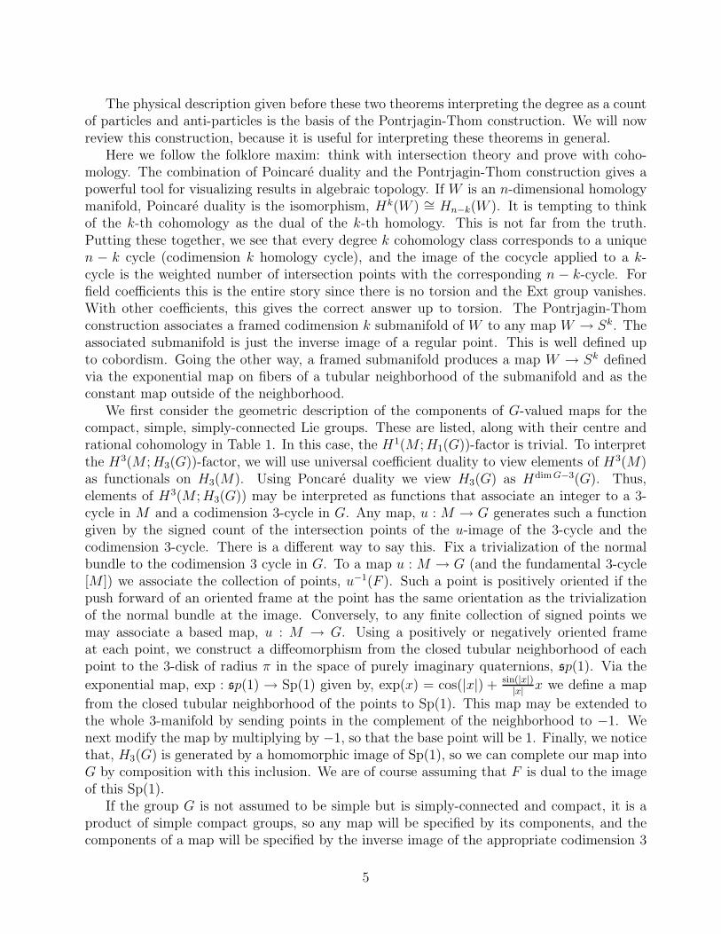
We first consider the geometric description of the components of G-valued maps for thecompact, simple, simply-connected Lie groups. These are listed, along with their centre andrational cohomology in Table 1. In this case, the H1(M ;H1(G))-factor is trivial. To interpretthe H3(M ;H3(G))-factor, we will use universal coefficient duality to view elements of H3(M)as functionals on H3(M). Using Poncare duality we view H3(G) as HdimG−3(G). Thus,elements of H3(M ;H3(G)) may be interpreted as functions that associate an integer to a 3-cycle in M and a codimension 3-cycle in G. Any map, u : M → G generates such a functiongiven by the signed count of the intersection points of the u-image of the 3-cycle and thecodimension 3-cycle. There is a different way to say this. Fix a trivialization of the normalbundle to the codimension 3 cycle in G. To a map u : M → G (and the fundamental 3-cycle[M ]) we associate the collection of points, u−1(F ). Such a point is positively oriented if thepush forward of an oriented frame at the point has the same orientation as the trivializationof the normal bundle at the image. Conversely, to any finite collection of signed points wemay associate a based map, u : M → G. Using a positively or negatively oriented frameat each point, we construct a diffeomorphism from the closed tubular neighborhood of eachpoint to the 3-disk of radius π in the space of purely imaginary quaternions, sp(1). Via the

exponential map, exp : sp(1) → Sp(1) given by, exp(x) = cos(|x|) + sin(|x|)|x|

x we define a map

from the closed tubular neighborhood of the points to Sp(1). This map may be extended tothe whole 3-manifold by sending points in the complement of the neighborhood to −1. Wenext modify the map by multiplying by −1, so that the base point will be 1. Finally, we noticethat, H3(G) is generated by a homomorphic image of Sp(1), so we can complete our map intoG by composition with this inclusion. We are of course assuming that F is dual to the imageof this Sp(1).

If the group G is not assumed to be simple but is simply-connected and compact, it is aproduct of simple compact groups, so any map will be specified by its components, and thecomponents of a map will be specified by the inverse image of the appropriate codimension 3

5

group, G center, Z(G) H∗(G; Q)An = SU(n+ 1), n ≥ 2 Zn+1 Q[x3, x5, . . . x2n+1]Bn = Spin(2n + 1), n ≥ 3 Z2 Q[x3, x7, . . . x4n−1]Cn = Sp(n), n ≥ 1 Z2 Q[x3, x7, . . . x4n−1]Dn = Spin(2n), n ≥ 4 Z2 ⊕ Z2 for even n Q[x3, x7, . . . x4n−5, y2n−1]

Z4 for odd nE6 Z3 Q[x3, x9, x11, x15, x17, x23]E7 Z2 Q[x3, x11, x15, x19, x23, x27, x35]E8 0 Q[x3, x15, x23, x27, x35, x39, x47, x59]F4 0 Q[x3, x11, x15, x23]G2 0 Q[x3, x11]

Table 1: Simple groups

cycles as described above. If the group is no longer assumed to be simply-connected we canassociate an element of H1(M ;H1(G0)) to any map u ∈ GM . This element maps a loop inM to a loop in G0 by composing with u. If u and v are two maps that generated the sameelement of H1(M ;H1(G0)), then u−1v will generate the trivial element, and so lifts to a mapto the universal covering group, G. The universal covering group of a Lie group is a product ofa vector space with a compact group, so up to homotopy this is a simply-connected, compactLie group. The homotopy class of the lift is specified by the element of H3(M ;H3(G)) asdescribed previously.

Given a map ϕ : M → S2, denote by (S2)Mϕ the set of all maps ψ ∈ (S2)M homotopic to

ϕ. The picture of the components of (S2)Mϕ arising from the Pontrjagin-Thom construction

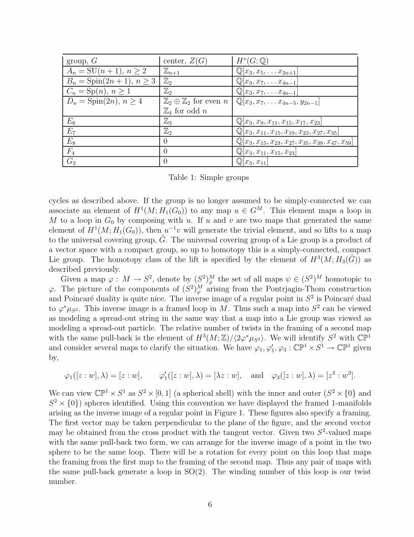
and Poincare duality is quite nice. The inverse image of a regular point in S2 is Poincare dualto ϕ∗µS2. This inverse image is a framed loop in M . Thus such a map into S2 can be viewedas modeling a spread-out string in the same way that a map into a Lie group was viewed asmodeling a spread-out particle. The relative number of twists in the framing of a second mapwith the same pull-back is the element of H3(M ; Z)/〈2ϕ∗µS2〉. We will identify S2 with CP1

and consider several maps to clarify the situation. We have ϕ1, ϕ′1, ϕ3 : CP1×S1 → CP1 given

by,

ϕ1([z : w], λ) = [z : w], ϕ′1([z : w], λ) = [λz : w], and ϕ3([z : w], λ) = [z3 : w3].

We can view CP1 ×S1 as S2 × [0, 1] (a spherical shell) with the inner and outer (S2 ×{0} andS2 × {0}) spheres identified. Using this convention we have displayed the framed 1-manifoldsarising as the inverse image of a regular point in Figure 1. These figures also specify a framing.The first vector may be taken perpendicular to the plane of the figure, and the second vectormay be obtained from the cross product with the tangent vector. Given two S2-valued mapswith the same pull-back two form, we can arrange for the inverse image of a point in the twosphere to be the same loop. There will be a rotation for every point on this loop that mapsthe framing from the first map to the framing of the second map. Thus any pair of maps withthe same pull-back generate a loop in SO(2). The winding number of this loop is our twistnumber.

6

Figure 1: Pontrjagin-Thom representatives of S2-valued maps

Figure 2: Introducing 2d twists

It may appear that there is a well-defined twist number associated to an S2-valued map.However, there is a homeomorphism of CP1×S1 twisting the 2-sphere (such a map is given by([z : w], λ) 7→ ([λz : w], λ)). This will change the apparent number of twists in a framing, butwill not change the relative number of twists. The reason why this relative number of twists isonly well defined modulo twice the divisibility of the cohomology class ϕ∗µS2 is demonstratedfor ϕ1 in Figure 2.

2.2 The fundamental group of configuration space

Where the components of the configuration space are typically labeled by the number ofparticles in the system, other topological properties of the configuration space may be used tomodel additional physical properties. We will next review the notion of statistics of particlesand describe one idea to use the fundamental group of configuration space to incorporatestatistics in a non-linear model.

Recall the distinction between bosons and fermions: a macroscopic ensemble of identicalbosons behaves statistically as if arbitrarily many particles can lie in the same state, while amacroscopic ensemble of identical fermions behaves as if no two particles can lie in the samestate. Photons are examples of particles with bosonic statistics and electrons are examples ofparticles with fermionic statistics. There are several theoretical models of particle statistics.In quantum mechanics, the wavefunction representing a multiparticle state is symmetric un-der exchange of any pair of identical bosons, and antisymmetric under exchange of any pairof identical fermions. In conventional perturbative quantum field theory, commuting fieldsare used to represent bosons and anti-commuting fields are used to represent fermions. Moreprecisely, bosons have commuting creation operators and fermions have anti-commuting cre-ation operators. However, there are times when fermions may arise within a field theory withpurely bosonic fundamental fields. This phenomenon is called emergent fermionicity, and itrelies crucially on the topological properties of the underlying configuration space of the model.

Emergent fermionic behavior may sometimes be explained on the basis of symmetry. Sym-metries of the classical configuration space, often imply symmetries of the space of quantumstates. However, the group of quantum symmetries can be different from the group of classicalsymmetries. It is this difference that may be used to explain emergent fermionicity, [5, chapter

7

7]. A spinning top is a well known example of this. The classical symmetry group is SO(3),while the quantum symmetry group for some quantizations is SU(2), [6, 21]. An electron inthe field of a magnetic monopole is also a good example, [5, chapter 7] and [9, 29].

When physical space is R3, so space-time is the usual Minkowski space, the classical ro-tational symmetries induce quantum symmetries that are representations of the Spin group.These irreducible representations are labeled by half integers (one half of the number of boxesin a Young diagram for a representation of SU(2)). The integral representations are honestrepresentations of the rotation group, but the fractional ones are not. The spin statistics the-orem states that any particle with fractional spin is a fermion, and any particle with integralspin is a boson.

The statistics of a particle may be viewed as a parity. A compound particle made out ofan even number of fermions will be a boson, and a compound particle comprised of an oddnumber of fermions will be a fermion. With this in mind, consider the fundamental group ofthe space of based maps from S3 to Sp(1).

The following figures show some loops in this configuration space. A loop in Sp(1)S3

isrepresented by a map from S3× [0, 1] to Sp(1). Such a map may be described by a framed loopin Sp(1)S3

. Fibers of the closed tubular neighborhood are mapped to Sp(1) via the exponentialmap, and the complement of this neighborhood can be mapped to the base point. This isexactly analogous to the correspondence between signed points in S3 and maps into Sp(1)described in the subsection on the components of Lie group valued-maps. The horizontaldirection in these figures represents the interval direction in S3 × [0, 1]. The disks representthe x − y plane and we suppress the z direction. Figure 3 shows two copies of a typicalloop representing an element in the fundamental group. Only the first vector of the framing isshown in Figure 3. The second vector is obtained by taking the cross product with the tangentvector to the curve in the displayed slice, and the final vector is the z-direction. It is easy to seethat the left copy may be deformed into the right copy. We describe the left copy as follows: aparticle and antiparticle are born; the particle undergoes a full rotation; the two particles thenannihilate. The right copy may be described as follows: a first particle-antiparticle pair is born;a second pair is born; the two particles exchange positions without rotating; the first particleand second antiparticle annihilate; the remaining pair annihilates. Notice that there are twoways a pair of particles can exchange positions. Representing the particles by people in a room,the two people may step sideways forwards/backwards and sideways following diametricallyopposite points on a circle always facing the back of the room. This is the exchange withoutrotating described in Figure 3. This exchange is non-trivial in π1(Sp(1)S3

). The second way apair of people may change positions is to walk around a circle at diametrically opposite pointsalways facing the direction that they walk to end up facing the opposite direction that theystarted. This second change of position is actually homotopically trivial. Since the framedlinks in Figure 3 avoid the slices, S3 × {0, 1}, they represent a loop based at the constantidentity map.

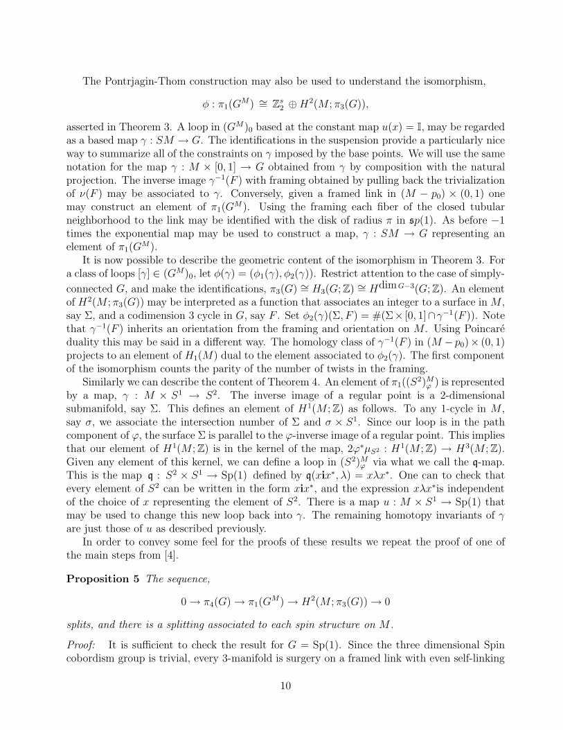
It is possible to describe a framing without drawing any normal vectors at all. The firstvector may be taken perpendicular to the plane of the figure, the second vector may be obtainedfrom the cross product with the tangent vector, and the third vector may be taken to be thesuppressed z-direction. The framing obtained by following this convention is called the blackboard framing. We use the blackboard framing in figure 4. The Pontrjagin-Thom construction

8

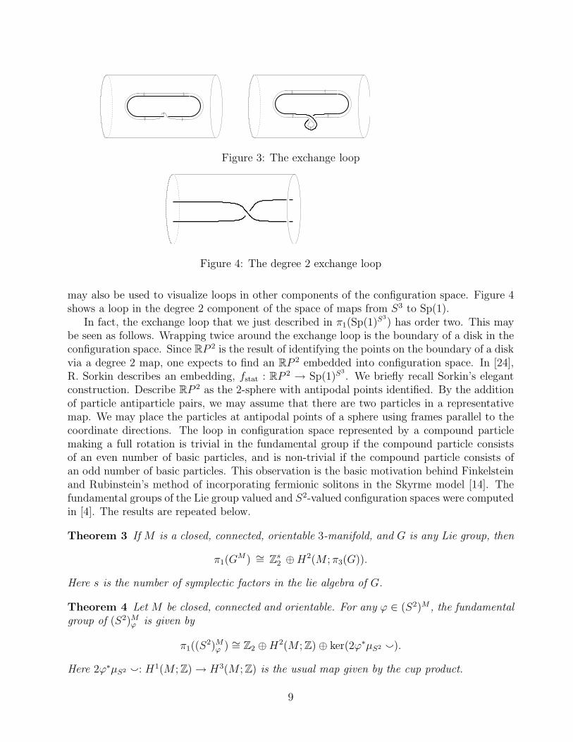
Figure 3: The exchange loop

Figure 4: The degree 2 exchange loop

may also be used to visualize loops in other components of the configuration space. Figure 4shows a loop in the degree 2 component of the space of maps from S3 to Sp(1).

In fact, the exchange loop that we just described in π1(Sp(1)S3

) has order two. This maybe seen as follows. Wrapping twice around the exchange loop is the boundary of a disk in theconfiguration space. Since RP 2 is the result of identifying the points on the boundary of a diskvia a degree 2 map, one expects to find an RP 2 embedded into configuration space. In [24],R. Sorkin describes an embedding, fstat : RP 2 → Sp(1)S3

. We briefly recall Sorkin’s elegantconstruction. Describe RP 2 as the 2-sphere with antipodal points identified. By the additionof particle antiparticle pairs, we may assume that there are two particles in a representativemap. We may place the particles at antipodal points of a sphere using frames parallel to thecoordinate directions. The loop in configuration space represented by a compound particlemaking a full rotation is trivial in the fundamental group if the compound particle consistsof an even number of basic particles, and is non-trivial if the compound particle consists ofan odd number of basic particles. This observation is the basic motivation behind Finkelsteinand Rubinstein’s method of incorporating fermionic solitons in the Skyrme model [14]. Thefundamental groups of the Lie group valued and S2-valued configuration spaces were computedin [4]. The results are repeated below.

Theorem 3 If M is a closed, connected, orientable 3-manifold, and G is any Lie group, then

π1(GM) ∼= Zs

2 ⊕H2(M ; π3(G)).

Here s is the number of symplectic factors in the lie algebra of G.

Theorem 4 Let M be closed, connected and orientable. For any ϕ ∈ (S2)M , the fundamentalgroup of (S2)M

ϕ is given by

π1((S2)M

ϕ ) ∼= Z2 ⊕H2(M ; Z) ⊕ ker(2ϕ∗µS2 `).

Here 2ϕ∗µS2 `: H1(M ; Z) → H3(M ; Z) is the usual map given by the cup product.

9

The Pontrjagin-Thom construction may also be used to understand the isomorphism,

φ : π1(GM) ∼= Zs

2 ⊕H2(M ; π3(G)),

asserted in Theorem 3. A loop in (GM)0 based at the constant map u(x) = I, may be regardedas a based map γ : SM → G. The identifications in the suspension provide a particularly niceway to summarize all of the constraints on γ imposed by the base points. We will use the samenotation for the map γ : M × [0, 1] → G obtained from γ by composition with the naturalprojection. The inverse image γ−1(F ) with framing obtained by pulling back the trivializationof ν(F ) may be associated to γ. Conversely, given a framed link in (M − p0) × (0, 1) onemay construct an element of π1(G

M). Using the framing each fiber of the closed tubularneighborhood to the link may be identified with the disk of radius π in sp(1). As before −1times the exponential map may be used to construct a map, γ : SM → G representing anelement of π1(G

M).It is now possible to describe the geometric content of the isomorphism in Theorem 3. For

a class of loops [γ] ∈ (GM)0, let φ(γ) = (φ1(γ), φ2(γ)). Restrict attention to the case of simply-

connected G, and make the identifications, π3(G) ∼= H3(G; Z) ∼= HdimG−3(G; Z). An elementof H2(M ; π3(G)) may be interpreted as a function that associates an integer to a surface in M ,say Σ, and a codimension 3 cycle in G, say F . Set φ2(γ)(Σ, F ) = #(Σ× [0, 1]∩γ−1(F )). Notethat γ−1(F ) inherits an orientation from the framing and orientation on M . Using Poincareduality this may be said in a different way. The homology class of γ−1(F ) in (M − p0)× (0, 1)projects to an element of H1(M) dual to the element associated to φ2(γ). The first componentof the isomorphism counts the parity of the number of twists in the framing.

Similarly we can describe the content of Theorem 4. An element of π1((S2)M

ϕ ) is representedby a map, γ : M × S1 → S2. The inverse image of a regular point is a 2-dimensionalsubmanifold, say Σ. This defines an element of H1(M ; Z) as follows. To any 1-cycle in M ,say σ, we associate the intersection number of Σ and σ × S1. Since our loop is in the pathcomponent of ϕ, the surface Σ is parallel to the ϕ-inverse image of a regular point. This impliesthat our element of H1(M ; Z) is in the kernel of the map, 2ϕ∗µS2 : H1(M ; Z) → H3(M ; Z).Given any element of this kernel, we can define a loop in (S2)M

ϕ via what we call the q-map.This is the map q : S2 × S1 → Sp(1) defined by q(xix∗, λ) = xλx∗. One can to check thatevery element of S2 can be written in the form xix∗, and the expression xλx∗is independentof the choice of x representing the element of S2. There is a map u : M × S1 → Sp(1) thatmay be used to change this new loop back into γ. The remaining homotopy invariants of γare just those of u as described previously.

In order to convey some feel for the proofs of these results we repeat the proof of one ofthe main steps from [4].

Proposition 5 The sequence,

0 → π4(G) → π1(GM) → H2(M ; π3(G)) → 0

splits, and there is a splitting associated to each spin structure on M .

Proof: It is sufficient to check the result for G = Sp(1). Since the three dimensional Spincobordism group is trivial, every 3-manifold is surgery on a framed link with even self-linking

10

njj

−1 −1

Figure 5: The 2-cycle

numbers [19]. Such a surgery description induces a Spin structure in M . Let M = S3L be such

a surgery description, orient the link and let {µj}cj=1 be the positively oriented meridians to

the components of the link. These meridians generate H1(M) ∼= H2(M ; π3(Sp(1))). This lastisomorphism is Poincare duality. Define a splitting by:

s : H1(M) → π1((Sp(1))M); s(µj) = PT (µj × {1

2}, canonical framing).

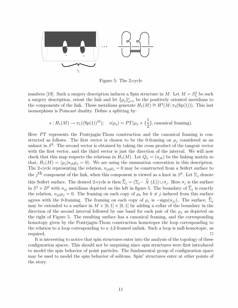
Here PT represents the Pontrjagin-Thom construction and the canonical framing is con-structed as follows. The first vector is chosen to be the 0-framing on µj considered as anunknot in S3. The second vector is obtained by taking the cross product of the tangent vectorwith the first vector, and the third vector is just the direction of the interval. We will nowcheck that this map respects the relations in H1(M). Let QL = (njk) be the linking matrix sothat, H1(M) = 〈µj|njkµj = 0〉. We are using the summation convention in this description.The 2-cycle representing the relation, njkµj = 0 may be constructed from a Seifert surface to

the jth component of the link, when this component is viewed as a knot in S3. Let Σj denote

this Seifert surface. The desired 2-cycle is then Σj = (Σj−◦

N (L))∪σj. Here σj is the surface

in S1 ×D2 with njj meridians depicted on the left in figure 5. The boundary of Σj is exactlythe relation, njkµj = 0. The framing on each copy of µk for k 6= j induced from this surface

agrees with the 0-framing. The framing on each copy of µj is −sign(njj). The surface, Σj

may be extended to a surface in M × [0, 1] × [0, 1] by adding a collar of the boundary in thedirection of the second interval followed by one band for each pair of the µj as depicted onthe right of Figure 5. The resulting surface has a canonical framing, and the correspondinghomotopy given by the Pontrjagin-Thom construction homotopes the loop corresponding tothe relation to a loop corresponding to a ±2-framed unlink. Such a loop is null-homotopic, asrequired. 2

It is interesting to notice that spin structures enter into the analysis of the topology of theseconfiguration spaces. This should not be surprising since spin structures were first introducedto model the spin behavior of point particles. The fundamental group of configuration spacemay be used to model the spin behavior of solitons. Spinc structures enter at other points ofthe story.

11

2.3 Rational cohomology of configuration space

The second cohomology of configuration space plays an important role in the quantum theory.The full rational cohomology may also appear as topological observables in the theory. Tosee the role of the second cohomology, recall some of the theory of geometric quantization[22]. In quantum theory one wishes to include the algebra of observables into the collectionof operators on some function space. Given a configuration manifold (space of positions), onedefines the phase space (collection of positions and momenta) to be the cotangent bundle ofconfiguration space. This has a canonical symplectic structure. The space of wave functions ischosen to be a set of sections of a complex line bundle over the quotient of phase space by anintegrable isotropic distribution of maximal dimension, the so-called polarization. The mostcommon choice is the vertical polarization, consisting of the tangent spaces to the fibres ofthe cotangent bundle. In this case, the quotient is naturally identified with the configurationspace itself.

There are many different complex line bundles over a space. Line bundles are in one to onecorrespondence with the elements of the second cohomology with integral coefficients. This iscalled quantization ambiguity in the physics literature. If we choose the vertical polarization,computing the quantization ambiguity requires one to consider the second integral cohomologyof configuration space. It is well-known that the second integral cohomology group may bedetermined from the fundamental group and the second rational cohomology group.

The real cohomology ring H∗((GM)0,R), including its multiplicative structure is describedin the following theorem from [4]. To state the theorem we will use a µ-map.

Similar to Yang-Mills theory, there is a µ-map,

µ : Hd(M ; R) ⊗Hj(G; R) → Hj−d(GM ; R),

and the cohomology ring is generated (as an algebra) by the images of this map. The µ mapproduces a (j − d)-cocycle in GM from a d-cycle in M and a j-cocycle in G. On the level ofchains, let ed : Dd →M be a d-cell, and xj be a closed j-form on G. Given a singular simplex,u : ∆j−d → GM , let u : M × ∆j−d → G be the natural map and write

µ(ed ⊗ xj)(u) =

∫

Dd×∆j−d

u∗xj .

Theorem 6 Let G be a compact, simply connected, simple Lie group. The cohomology ringof any of these groups is a free graded-commutative unital algebra over R generated by degreek elements xk for certain values of k (and with at most one exception at most one generatorfor any given degree). The values of k depend on the group and are listed in Table 1 in section2.1. Let M be a closed, connected, orientable 3-manifold. The cohomology ring H∗((GM)0; R)is the free graded-commutative unital algebra over R generated by the elements µ(Σd

j ⊗ xk),where Σd

j form a basis for Hd(M ; R) for d > 0 and k − d > 0.

We also have the rational cohomology of (S2)M from [4].

Theorem 7 Let M be closed, connected and orientable, let ϕ : M → S2, let Σdj form a

basis for Hd(M ; R) for d < 3, and let {αk} for a basis for ker(2ϕ∗µS2 `: H1(M ; Z) →

12

H3(M ; Z)). The cohomology ring H∗((S2)Mϕ ; R) is the free graded-commutative unital algebra

over R generated by the elements αk and µ(Σdj ⊗x), where x ∈ H3(Sp(1); Z) is the orientation

class. The classes αk have degree 1 and µ(Σdj ⊗ x) have degree 3 − d.

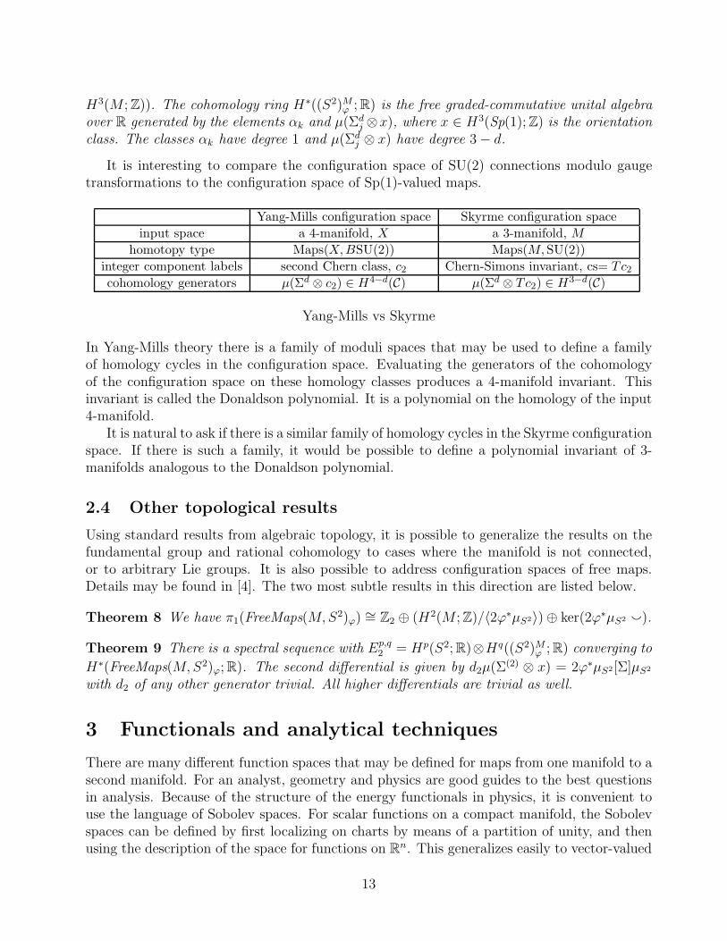
It is interesting to compare the configuration space of SU(2) connections modulo gaugetransformations to the configuration space of Sp(1)-valued maps.

Yang-Mills configuration space Skyrme configuration space

input space a 4-manifold, X a 3-manifold, M

homotopy type Maps(X,BSU(2)) Maps(M,SU(2))

integer component labels second Chern class, c2 Chern-Simons invariant, cs= Tc2

cohomology generators µ(Σd ⊗ c2) ∈ H4−d(C) µ(Σd ⊗ Tc2) ∈ H3−d(C)

Yang-Mills vs Skyrme

In Yang-Mills theory there is a family of moduli spaces that may be used to define a familyof homology cycles in the configuration space. Evaluating the generators of the cohomologyof the configuration space on these homology classes produces a 4-manifold invariant. Thisinvariant is called the Donaldson polynomial. It is a polynomial on the homology of the input4-manifold.

It is natural to ask if there is a similar family of homology cycles in the Skyrme configurationspace. If there is such a family, it would be possible to define a polynomial invariant of 3-manifolds analogous to the Donaldson polynomial.

2.4 Other topological results

Using standard results from algebraic topology, it is possible to generalize the results on thefundamental group and rational cohomology to cases where the manifold is not connected,or to arbitrary Lie groups. It is also possible to address configuration spaces of free maps.Details may be found in [4]. The two most subtle results in this direction are listed below.

Theorem 8 We have π1(FreeMaps(M,S2)ϕ) ∼= Z2 ⊕ (H2(M ; Z)/〈2ϕ∗µS2〉) ⊕ ker(2ϕ∗µS2 `).

Theorem 9 There is a spectral sequence with Ep,q2 = Hp(S2; R)⊗Hq((S2)M

ϕ ; R) converging to

H∗(FreeMaps(M,S2)ϕ; R). The second differential is given by d2µ(Σ(2) ⊗ x) = 2ϕ∗µS2[Σ]µS2

with d2 of any other generator trivial. All higher differentials are trivial as well.

3 Functionals and analytical techniques

There are many different function spaces that may be defined for maps from one manifold to asecond manifold. For an analyst, geometry and physics are good guides to the best questionsin analysis. Because of the structure of the energy functionals in physics, it is convenient touse the language of Sobolev spaces. For scalar functions on a compact manifold, the Sobolevspaces can be defined by first localizing on charts by means of a partition of unity, and thenusing the description of the space for functions on Rn. This generalizes easily to vector-valued

13

functions. To define a Sobolev space of functions taking values in a manifold (say N), onetakes an isometric embedding of N into a vector space and considers those elements of theSobolev space taking values in the vector space that lie in N almost everywhere. We denoteby W s,p(M, N) the Sobolev space of maps from M to N which have s derivatives in Lp.

3.1 Local representation of functions by flat connections

One idea that has proven to be useful in the study of non-linear models has been a localrepresentation of functions by flat connections. This first shows up when the codomain is aLie group. Given a smooth map u : M → G one can construct the Lie algebra valued 1-formA = u−1du. This form satisfies dA + A ∧ A = 0 and can be interpreted as a flat connection.Conversely, given a flat connection defined on a cube In one may define a function u : In → Gby solving the parallel transport equation du(γ(t)) = u(γ(t))A(γ(t)) with u(x0) = I. It followsfrom the fact that A is flat that the value u(γ(1)) does not depend on the path connectingx0 to γ(1). Changing the initial value or base point will change the function u by a constantmultiple. The same result holds for L2 connections, [1], but the proof is much more involved.The result from [1] reads:

Theorem 10 Given any L2 g-valued 1-form A on Im such that

dA +1

2[A, A] = 0 (3.1)

in the sense of distributions, there exists u ∈W 1,2(Im, G) such that u−1 ∈W 1,2(Im, G) andA = u−1 du. Furthermore, for any two such maps, u and v, there exists g ∈ G so thatu(x) = g · v(x), for almost every x ∈ Im.

The second local representation theorem is proved in [3] for S2-valued maps. It reads:

Theorem 11 If ϕ is in W 1,3(I3, S2) or W 1,2E (I3, S2) then there is a u ∈ W 1,3(I3, Sp(1))

or u ∈ W 1,2(I3, Sp(1)) respectively so that ϕ = u∗ i u. In either case Re((u∗du)3) ∈ L1.Furthermore, for any two such maps u and v there is a map λ in W 1,3(I3, S1) or W 1,2(I3, S1)respectively, so that v = λu.

The space W 1,2E (I3, S2) was defined to analyze the Faddeev model. We will recall its definition

in a subsection below. The map Sp(1) → S2 given by u 7→ u∗iu is a convenient way to expressthe quotient projection Sp(1) → Sp(1)/S1. More generally, if H is a closed subgroup of aLie group G then functions from In to G/H may be factored through G. This will appear infuture work. There is an important class of sigma models in physics called coset models wherethe target is a homogenous space G/H . The G-valued map may then be represented by a flatconnection as before.

It is possible that the same ideas could be used to represent functions taking values in anarbitrary manifold, N . The diffeomorphisms on any manifold act transitively. This meansthat given any pair of points x0, x1 there is a diffeomorphism with f(x0) = x1. Let Diff(N)denote the topological group of all diffeomorphisms, and let Stabx0

denote the closed subgroupconsisting of all diffeomorphisms fixing x0. It is not difficult to see that there is a homeomor-phism Diff(N)/Stabx0

∼= N . Thus we could try the same idea, factor a map into N through

14

Diff(N) and then represent a Diff(N)-valued map by a flat connection. The cost in this typeof representation is that the structure group is infinite dimensional in this general case. Suchissues have been addressed in gauge theory, so it is worth remembering this possibility, becauseit may someday find application.

3.2 Homotopy theory for finite energy maps

Our first application of these local representation theorems will be to the study of homotopytheory in classes of maps with finite energy. This question naturally arises because one commonfeature among many sigma models is the restriction to a fixed homotopy class. The homotopyclasses divide the particles into different sectors, and numerical invariants distinguishing theclasses (sectors) bear some definite physical meaning (depending on the model). Good physicalmodels describe interesting physics and have energy functionals that respect geometry of theconfiguration space.

There has been a fair amount of work done relating homotopy theory to Sobolev spacesW s,p(M,N), see [8] for a review of recent results. A paraphrase of the result of White [27]gives a good idea of what to expect: The homotopy classes of maps with one derivativein Lp restricted to the k-skeleton of a manifold agree with the homotopy classes of smoothmaps provided k is less than p. For example, the second cohomology of a space is completelydetermined by the homotopy classes of maps from the 3-skeleton of the space into a K(Z, 2) (orCPN for N sufficiently large). Thus one would expect the pull-back of a second cohomologyclass under a W 1,3 map to be well defined. In general, the third cohomology of a space dependson the 4-skeleton, of course if the space is a 3-manifold, then the 3-skeleton will suffice and thepull-back will be well defined for W 1,3 maps. Similarly one would expect the Hopf invariantto be well defined for W 1,3 maps.

In this paper we consider two energy functionals corresponding to the Skyrme and Faddeevmodels. The Skyrme functional for maps u : M → G is defined to be

E(u) =

∫

M

1

2|u−1 du|2 +

1

4|u−1 du ∧ u−1 du|2 d volM . (3.2)

Skyrme originally considered this in the case of maps from R3 to SU(2), [23]. We describedthe physical interpretation of these maps in the section on topology.

The Faddeev functional is defined for maps ψ : M → S2 as follows, [10]:

E(ψ) =

∫

M

|dψ|2 + |dψ ∧ dψ|2 dvol . (3.3)

It is related to the Skyrme functional: viewing S2 as an equator in the 3-sphere SU(2), theFaddeev functional is just the restriction of the SU(2)-Skyrme functional to S2-valued mapsψ(x) = ψ1(x) i + ψ2(x) j + ψ3(x)k.

For these two models, the finite energy maps are those u ∈W 1,2(M,G) or ψ ∈W 1,2(M,S2)for which E(u) or E(ψ) are finite. We denote such classes of maps by W 1,2

E .It is useful to keep several explicit maps in mind when considering the homotopy theory

of maps in generalized function spaces. First consider the map from the 3-disk to the 2-sphere η1 : D3 → S2 given by, η1(x) = x/|x|. Simple integration suffices to verify that

15

η1 is in W 1,p for p < 3, but is not in W 1,2E or W 1,3. Notice that the integral of the η1-

pull-back of the normalized area form on S2 integrates to 1 on the boundary of D3. Thusthe pull-back on second cohomology may not be reasonably defined for such maps. Evenmore regularity is required to define the pull-back on the third cohomology. The compositionof projection of S3 to D3 with this η1 map may be patched into any smooth map from a3-manifold to obtain a similar example. Similarly the function, η2 : D3 → S1 given byη2(x) = cos(ln |x|)i + sin(ln |x|)j is in W 1,p

E for p < 3 but not in W 1,3, and the functionη3 : D3 → S1 given by η3(x) = cos(ln | ln |x/e||)i + sin(ln | ln |x/e||)j is in W 1,3 but is notcontinuous. These two last functions may also be patched into maps from an arbitrary 3-manifold. Furthermore they may be composed with maps into any non-trivial compact Liegroup or into S2.

Our applications of the local representation theorems to homotopy problems are similar tothe definition of Cech cohomology. As our first example, consider the space of flat connectionsmodulo gauge equivalence. It is well known that the path components are labeled by theholonomy representation.

It is possible to define the holonomy for L2loc distributionally flat connections. Recall from

the sample functions listed above that the local developing maps for such a connection can looklike Swiss cheese. Here is a sketch of the definition. Given a sufficiently fine cover of a manifoldby cubes, the nerve of the cover will be homotopy equivalent to the manifold. (The nerve isa complex with one vertex for each cube, an edge for each non-empty intersection, trianglefor each non-empty triple intersection etc.) The edge path group of a complex is an analogueof the fundamental group of a topological space. It is isomorphic to the fundamental groupof the topological realization of the complex. Given an L2

loc distributionally flat connection,say A, we can find local developing maps up such that A = u−1

p dup on each cube by the localrepresentation theorem. Furthermore, each edge of the nerve may be labeled by the groupelement relating the two local developing maps. This gives a representation of the edge pathgroup. The actual definition includes the transition functions of the bundle supporting theconnection, and is only valid for central bundles. It is an open question to generalize thedefinition of holonomy to arbitrary flat connections, see [1].

Using the notion of holonomy, it is possible to generalize the local representation theoremto a global representation theorem.

Lemma 12 Two L2loc distributionally flat connections on a central bundle are gauge equiva-

lent if and only if they have the same holonomy.

The homotopy invariant of a map from M to G living in H1(M ;H1(G0)) may be interpretedas the holonomy of a flat connection, and therefore is well-defined for W 1,2 maps.

There are similar applications of the local representation theorem for S2-valued maps.Given a smooth map ϕ : M → S2 one may construct the pull-back of the orientation classµS2 ∈ H2(S2; Z). This class ϕ∗µS2 ∈ H2(M ; Z) is also the obstruction to lifting the map ϕ toa map u : M → Sp(1) such that ϕ = uiu∗. Using the Cech picture and the local representationtheorem, one may define the obstruction class for W 1,3 or W 1,2

E maps. Using this obstructionwe can prove the following global representation theorem, see [2, 3].

16

Proposition 13 If ϕ and ψ are two maps in W 1,3(M,S2) or W 1,2E (M,S2) then there is a w in

W 1,3(M, Sp(1)) or w ∈W 1,2(M, Sp(1)) respectively with∫

MRe((w∗dw)3) <∞ and ψ = wϕw∗

if and only if ϕ∗µS2 = ψ∗µS2. If w1 and w2 are two such maps, then there is a λ in W 1,3(M,S1)or in W 1,2(M,S1) respectively with w1 = qw2.

The proof of this lifting theorem is similar to the proof of local gauge slices in gauge theory.The geometry suggests a natural system of differential equations that may be solved to givethe lift.

Using de Rham theory, some homotopy invariants may be represented as integrals of differ-ential forms. When an invariant is integral, this is the first thing anyone would try. Invariantsliving in the top cohomology are usually represented in this way. Sometimes a homotopyinvariant takes values in a group with torsion. There are two ways we address torsion. We usethe Cech picture as we described above, or we lift the map to a different space and realize thetorsion invariant of the original map as an integral invariant of the lift. Torsion is introducedin this second picture when there is more than one possible lift. In any such application ofde Rham theory there is a new issue that arises. The de Rham cohomology is cohomologywith real coefficients and the integral is the cap product. Thus a priori such integrals are onlyknown to be real numbers. It is possible to use the local representation theorems to provethat these integrals take integral values, even for Sobolev maps. Some sample theorems from[3] are listed below.

Theorem 14 Let G be a compact, simply-connected Lie group, let M be a closed oriented3-manifold, let Θ be a smooth form representing an integral class in H3(G), and let u be amap in W 1,3(M,G) or in W 1,2

E (M,G). Then the number∫

Mu∗Θ is an integer.

It follows that the H3(M ;H3(G)) invariants of homotopy classes of maps from M to Gare integers for Sobolev maps and general compact Lie groups. By lemma 12, any L2

loc dis-tributionally flat connection is gauge equivalent to a smooth connection. The Chern-Simonsinvariants of these two connections are related by the degree of the gauge transformation, sowe have the following corollary.

Corollary 15 If A is a finite energy distributionally flat L2 connection on a central bundlethen there is a smooth connection on the same bundle with the same holonomy and Chern-Simons invariant.

This integrality proposition combines with the lifting theorem for S2-valued maps to givea version of the secondary invariant for Sobolev S2-valued maps. We need a second integralityresult to know that the degree of the lift changes by multiples of the right amount when thelift is changed. This is the content of the next result.

Proposition 16 When ψ and λ are in W 1,3 or when ψ is in W 1,2E and λ is in W 1,2, the

expression − 116π2i

∫Mψdψ ∧ dψλ∗dλ is an integer.

Here is the formal definition of the secondary homotopy invariant for Sobolev S2-valued maps.

17

Definition 17 Given ϕ, ψ : M → S1 in W 1,3 or in W 1,2E such that ϕ∗µS2 = ψ∗µS2 define

Υ(ϕ, ψ) = −1

12π2

∫

M

Re((w∗dw)3) ∈ Z2mψ,

where w is the map given by Proposition 13.

It follows from Theorem 14 that Υ is an integer. To see that Υ is well defined notice that

−1

12π2

∫

M

Re(((wq(ψ, λ)∗dw)3) = −1

8π2i

∫

M

ψdψ ∧ dψλ∗dλ−1

12π2

∫

M

Re((w∗dw)3).

See [2] for a proof of this. These invariants serve to generalize Pontrjagin’s theorem to Sobolevmaps or finite energy maps because two smooth S2-valued maps ϕ and ψ are homotopic ifand only if ϕ∗µS2 = ψ∗µS2 and Υ(ϕ, ψ) = 0.

Our expression for Υ generalizes an integral formula for the Hopf invariant, see [7]. Indeed,when ϕ∗µS2 is torsion (in particular if M = S3), the pull-back, ϕ∗ωS2, of the volume form onS2 is exact and there is a 1-form, θϕ, so that dθϕ = ϕ∗ωS2. The Hopf invariant of ϕ is thendefined to be

∫Mθϕdθϕ. The following proposition relates the Hopf invariant and Υ.

Proposition 18 Let ϕ, ψ : M → S2 in W 1,3 or in W 1,2E such that R ϕ∗µS2 = 0 for some non

zero integer. For the minimal positive R, we have

Hopf (ϕ) =1

RΥ(ϕR, i),

where ϕR is the composition of ϕ with the map z 7→ zR of S2 to itself.

Thus we see that our generalization of Pontrjagin’s theorem for Sobolev maps specializes toan integrality result for the Hopf invariant of Sobolev maps.

3.3 Minimizing functionals

One motivation for our study of the topology of spaces of maps and extensions to Sobolevmaps was to consider minimization problems for the Skyrme and Faddeev functionals. Inphysical lingo, the minimizers of the energy functional (in every sector) are called the groundstates. Their geometric structure and stability are of great importance. The reader may findinteresting pictures and discussion of purported ground states for the original Skyrme modelin [15] and for the Faddeev model in [12] and [17].

In this subsection we will present our results establishing the existence of minimizers andcompactness of the set of minimizers for the Skyrme and Faddeev functionals. Along withthe energy functionals for maps, (3.2) and (3.3), we consider functionals for connections. In[23], Skyrme noticed and used the fact that maps could be represented by flat connections,a = u−1du. This leads to a second version of the Skyrme functional,

E[a] =

∫

M

1

2|a|2 +

1

16|[a, a]|2 d volM . (3.4)

18

The Faddeev functional can be also written in terms of flat connections, [2]. Given a smoothreference map ϕ : M → S2, any ψ homotopic to ϕ, can be represented as ψ = uϕu∗ withu : M → Sp(1). Plugging this expression into the energy functional, using Ad-invariance ofthe norm and the Lie bracket, and the notation a = u∗ du , we obtain

E(ψ) = Eϕ[a] :=

∫

M

|Daϕ|2 + |Daϕ ∧Daϕ|

2 , (3.5)

where Daϕ = dϕ + [a, ϕ]. As was observed in [18, 1, 2], the variational problems formaps and for connections are, in general, different. The way we approach these variationalproblems requires several steps, [1, 2]. First, we describe the homotopy classes for smoothmaps and analytically define expressions to label different classes. Second, we show that thoseexpressions for labels of the components extend to finite energy Sobolev maps (or connections).Third, we show that there exist minimizers in every sector of finite energy maps specified bygiven values of the label. We also prove in [3] that the values these labels take on finite energyconfigurations agree with the possible values on smooth configurations.

There is an open question remaining related to the components of the spaces W 1,2E : The set

of finite energy maps (or connections) with a fixed label is not known to be path connected.So we call such sets sectors. We expect that the sectors are the components of the spaces offinite energy maps when a suitable topology is used.

The existence of minimizers is established by the direct method of the calculus of variations,so given a sequence of maps in a fixed sector with energy approaching the infimum, there isa subsequence converging to a minimizer in the same sector. In particular, any sequence ofminimizers in a fixed sector contains a convergent subsequence, hence the set of minimizers ofthe Skyrme or Faddeev functional in a fixed sector is compact in W 1,2

E .

Future work will address the existence of minimizers of a generalized Skyrme functionalfor maps into general homogenous spaces. We also plan to study the regularity. It is commonfor minimizers of a functional in a class of functions to be more regular than generic membersof the class. We expect to see applications of the local representation results for functions tothe regularity of minimizers.

One may speculate that the minimizers of the Skyrme functional may form a cycle in theconfiguration space of maps from M to G. Given such a cycle one could evaluate cohomologyclasses from the configuration space to obtain topological invariants. We believe that this isslightly nave because the Skyrme functional lacks an important property shared by functionalthat do serve to define invariants of manifolds. Recall that sufficiently regular minimizers offunctionals similar to the Skyrme functional satisfy second order Euler-Lagrange equations.When a functional is topologically saturated, the minimizers are characterized as the solutionsof a first order system of equations. For example, the anti-self dual condition in Yang-Mills the-ory, the pseudoholomorphic condition in Gromov-Witten theory, or Sieberg-Witten equationsin Seiberg-Witten theory are all examples of first order systems characterizing minima. Onecan write out what the first order equations corresponding to the Skyrme functional shouldbe. However, these equations are overdetermined and essentially have no solutions. Theequations are analogous to what one would have by considering the Seiberg-Witten equationsfor a fixed connection and attempting to solve for the spin field. We believe that a suitable

19

modification of the Skyrme functional incorporating new fields (perhaps gauge bosons?) willbe topologically saturated and may lead to new smooth invariants of manifolds.

References

[1] Auckly, D., Kapitanski, L.: Holonomy and Skyrme’s Model. Commun. Math. Phys. 240,97–122 (2003)

[2] Auckly, D., Kapitanski, L.: Analysis of the Faddeev Model. Commun. Math. Phys. ac-cepted. (http://arxiv.org/abs/math-ph/040302)

[3] Auckly, D., Kapitanski, L.: Integrality of invariants for Sobolev maps. In progress.

[4] Auckly, D., Speight, J.M.: Fermionic quantization and configuration spaces for theSkyrme and Faddeev-Hopf models. preprint. (http://arxiv.org/abs/hep-th/0411010)

[5] Balachandran, A., Marmo, G., Skagerstam, B., Stern, A.: Classical topology and quantumstates. New Jersey : World Scientific, 1991

[6] Bopp, F., Haag, Z.: Uber die moglichkeit von spinmodellen. Zeitschrift fur Natur-forschung 5a, 644 (1950)

[7] Bott, R., Tu, L.W.: Differential forms in algebraic topology. New York : Springer-Verlag,1982

[8] Brezis, H.: The interplay between analysis and topology in some nonlinear PDE problems.Bull. Amer. Math. Soc. (N.S.) 40, no. 2, 179–201 (2003)

[9] Dirac, P.: The theory of magnetic poles. Phys. Rev. 74, 817–830 (1948)

[10] Faddeev, L. D.: Quantization of solitons. Preprint IAS print-75-QS70 (1975)

[11] Faddeev, L. D.: Knotted solitons and their physical applications. Phil. Trans. R. Soc.Lond. A 359, 1399–1403 (2001)

[12] Faddeev, L. D., Niemi, A. J.: Stable knot-like structures in classical field theory. Nature387, 58–61 (1997)

[13] Federer, H.: A study of function spaces by spectral sequences. Ann. of Math. 61, 340-361(1956)

[14] Finkelstein, D., Rubunstein,J,: Connection between spin statisitics and kinks. J. Math.Phys. 9, 1762–1779 (1968)

[15] Gisiger, T., Paranjape, M. B.: Recent mathematical developments in the Skyrme model.Phys. Rep. 306, no. 3, 109–211 (1998)

[16] Giulini, D.: On the possibility of spinorial quantization in the Skyrme model. Mod. Phys.Lett. A8, 1917–1924 (1993)

20

[17] Hietarinta J., Salo P.: Ground state in the Faddeev-Skyrme model. Phys. Rev. D 62,081701(R) (2000)

[18] Kapitanski, L.: On Skyrme’s model, in: Nonlinear Problems in Mathematical Physicsand Related Topics II: In Honor of Professor O. A. Ladyzhenskaya, Birman et al., eds.Kluwer, 2002, pp.229-242

[19] Kirby, R.C.: The topology of 4-manifolds. Lecture Notes in Mathematics 1374, New York: Springer-Verlag, 1985

[20] Pontrjagin, L.: A classification of mappings of the 3-dimensional complex into the 2-dimensional sphere. Mat. Sbornik N.S. 9:51, 331-363 (1941)

[21] Schulman, L.: A path integral for spin. Phys. Rev. 176:5, 1558-1569 (1968))

[22] Simms, D.J., Woodhouse, N.M.J.: Geometric quantization. Lecture Notes in Physics 53,Berlin: Springer-Verlag, 1977

[23] Skyrme, T.H.R.: A unified field theory of mesons and baryons. Nucl. Phys. 31, 555–569(1962)

[24] Sorkin, R.: A general relation between kink-exchange and kink-rotation. Commun. Math.Phys. 115, 421–434 (1988)

[25] Vakulenko, A. F., Kapitanski, L.: On S2-nonlinear σ-model. Dokl. Acad. Nauk SSSR248, 810–814 (1979)

[26] Weinberg, S.: The quantum theory of fields. Cambridge : Cambridge University Press,1995

[27] White, B.: Homotopy classes in Sobolev spaces and the existence of energy minimizingmaps, Acta Mathematica 160, 1-17 (1988)

[28] Witten, E.: Current algebra, baryons and quark confinement. Nucl. Phys. B233, 433–444(1983)

[29] Zaccaria, F., Sudarshan, E., Nilsson, J., Mukunda, N., Marmo, G., Balachandran, A.:Universal unfolding of Hamiltonian systems: from symplectic structures to fibre bundles.Phys. Rev. D27, 2327-2340 (1983)

21