Geometric Mechanics of Periodic Pleated Origami

Z.Y. Wei,1 Z. V. Guo,1 L. Dudte,1 H.Y. Liang,1 and L. Mahadevan1,2,*1School of Engineering and Applied Sciences, Harvard University, Cambridge, Massachusetts 02138, USA

2Department of Physics, Harvard University, Cambridge, Massachusetts 02138, USA(Received 25 November 2012; revised manuscript received 16 February 2013; published 21 May 2013)

Origami structures are mechanical metamaterials with properties that arise almost exclusively from the

geometry of the constituent folds and the constraint of piecewise isometric deformations. Here we

characterize the geometry and planar and nonplanar effective elastic response of a simple periodically

folded Miura-ori structure, which is composed of identical unit cells of mountain and valley folds with

four-coordinated ridges, defined completely by two angles and two lengths. We show that the in-plane and

out-of-plane Poisson’s ratios are equal in magnitude, but opposite in sign, independent of material

properties. Furthermore, we show that effective bending stiffness of the unit cell is singular, allowing us to

characterize the two-dimensional deformation of a plate in terms of a one-dimensional theory. Finally, we

solve the inverse design problem of determining the geometric parameters for the optimal geometric and

mechanical response of these extreme structures.

DOI: 10.1103/PhysRevLett.110.215501 PACS numbers: 81.05.Xj, 46.70.De

Metamaterials are defined as materials whose structureand constitution allows them to have unusual emergentproperties, such as negative refractive index opticalmetamaterials [1], or negative Poisson ratio mechanicalmetamaterials [2]. Here, we focus on origami-inspiredmechanical metamaterials that arise as folded and pleatedstructures in a variety of natural systems including insectwings [3], leaves [4], and flower petals [5]. Using thepresence of creases in these systems allows one to foldand unfold an entire structure simultaneously and designdeployable structures such as solar sails [6] and foldablemaps [7], and auxetic structural materials such as foams[8], and microporous polymers [9]. Indeed, folded sheetswith reentrant geometries serve as models for crystal struc-tures [10,11], molecular networks [12], and glasses [2] ina variety of physical applications. Complementing thesestudies, there has been a surge of interest in the mathe-matical properties of these folded structures [13–15], andsome recent qualitative studies on the engineering aspectsof origami [16–18]. In addition, the ability to create themde novo without a folding template, as a self-organizedbuckling pattern when a stiff skin resting on a soft founda-tion is subject to biaxial compression [19–21] has openedup a range of questions associated with their assemblyin space and time, and their properties. However, mostpast quantitative work on these materials has been limitedto understanding their behavior in two dimensions, eitherby considering their auxetic behavior in the plane, or thebending of a one-dimensional corrugated strip. In thisLetter, we characterize the three-dimensional elasticresponse, Poisson’s ratios, and rigidities of perhaps thesimplest suchmechanicalmetamaterial based on origami—a three-dimensional periodically pleated or folded struc-ture, the Miura-ori pattern, [Fig. 1(a)] which is definedcompletely in terms of two angles and two lengths.

The geometry of the unit cell embodies the basic ele-ment in all nontrivial pleated structures—the mountainor valley fold, wherein four edges (folds) come togetherat a single vertex, as shown in Fig. 1(d). It is parametrizedby two dihedral angles 2 ½0; , 2 ½0; , and oneoblique angle , in a cell of length l, widthw, and height h.We treat the structure as being made of identical periodicrigid skew plaquettes joined by elastic hinges at the ridges.The structure can deploy uniformly in the plane [Fig. 1(b)]by having each constituent skew plaquette in a unit cell

(b)

(a) (c)

(d)

FIG. 1 (color online). Geometry of Miura-ori pattern. (a) AMiura-ori plate folded from a letter size paper contains 13 by 13unit cells (along x and y directions, respectively), with ¼ 45and l1 ¼ l2 ¼ le. The plate dimension is 2L by 2W. (b) In-planestretching behavior of a Miura-ori plate when pulled along the xdirection shows it expands in all directions; i.e., it has a negativePoisson’s ratio. (c) Out-of-plane bending behavior of a Miura-oriplate when a symmetric bending moment is applied on bounda-ries x ¼ L shows a saddle shape, consistent with that, in thismode of deformation, its Poisson’s ratio is positive. (d) Unit cellof Miura-ori is characterized by two angles and given l1 andl2 and is symmetric about the central plane passing throughO1O2O3.

PRL 110, 215501 (2013) P HY S I CA L R EV I EW LE T T E R Sweek ending24 MAY 2013

0031-9007=13=110(21)=215501(5) 215501-1 2013 American Physical Society

rotate rigidly about the connecting elastic ridges. Thenthe ridge lengths l1, l2, and 2 ½0; =2 are constantthrough folding or unfolding, so that we may choose (or equivalently ) to be the only degree of freedom thatcompletely characterizes a Miura-ori cell. The geometry ofthe unit cell implies that

¼ 2sin1½ sinð=2Þ; l ¼ 2l1;

w ¼ 2l2 and h ¼ l1 tan cosð=2Þ;(1)

where the dimensionless width and height are

¼ sin sinð=2Þ and ¼ cosð1 2Þ1=2: (2)

We see that , l, w, and h change monotonically as 2 ½0; , with 2 ½0; , l 2 2l1½cos; 1, w 22l2½0; sin, and h 2 l1½sin; 0. As 2 ½0; =2, wesee that 2 ½; 0, l 2 ½2l1; 0, w 2 ½0; 2l2 sinð=2Þ,and h 2 ½0; l1. The geometry of the unit cell impliesa number of interesting properties associated with theexpansion kinematics of a folded Miura-ori sheet, includ-ing design optimization for packing, and the study ofnearly orthogonal folds when =2, the singular casecorresponding to the common map fold where the foldsare all independent (SI-1 in Supplemental Material [22]).To minimize algebraic complexity and focus on the mainconsequences of isometric deformations of these struc-tures, we will henceforth assume each plaquette is a rhom-bus, i.e., l1 ¼ l2 ¼ le.

The planar response of Miura-ori may be characterizedin terms of two quantities—the Poisson’s ratio whichdescribes the coupling of deformations in orthogonal direc-tions, and the stretching rigidity which characterizes itsplanar mechanical stiffness. The linearized planarPoisson’s ratio is defined as

wl dw=w

dl=l¼ 1 2: (3)

It immediately follows that the reciprocal Poisson’s ratiolw ¼ 1=wl. Because 1, the in-plane Poisson’s ratiowl < 0 [Fig. 2(a)]; i.e., Miura-ori is an auxetic material.The limits on wl may be determined by considering theextreme values of , , since wl monotonically increasesin both variables. Using the expression (2) in (3) andexpanding the result shows that wlj!0 2, and thus,wlj 2 ð1;cot2ð=2Þ, while wlj!0 2 and,thus, wlj 2 ð1;cot2. When ð; Þ ¼ ð=2; Þ,wl ¼ 0 so that the two orthogonal planar directionsmay be folded or unfolded independently, as in traditionalmap folding. Indeed, this is the unique state for whichnonparallel folds are independent, and it might surprisethe reader that, with few exceptions, this is the way mapsare folded—makes unfolding easy, but folding frustrating!The Poisson’s ratios related to height changes, hl andwh can also be determined using similar arguments(SI-2.1 in Supplemental Material [22]).

To calculate the in-plane stiffness of the unit cell,we note that the potential energy of a unit cell deformedby a uniaxial force fx in the x direction is H ¼U R

0fxðdl=d0Þd0, assuming that the elastic energy

of a unit cell is stored only in the elastic hinges whichallow the rigid plaquettes to rotate isometrically, withU ¼ kleð 0Þ2 þ kleð 0Þ2, k being the hingespring constant, 0 and 0 ½¼ ð; 0Þ being the naturaldihedral angles in the undeformed state. Then, the externalforce fx at equilibrium is determined by the relationH= ¼ 0, while the stretching rigidity in the x directionis given by

Kxð;0Þdfxd

0

¼ 4k½ð120Þ2þcos2

ð120Þ1=2 cossin2sin0

; (4)

where 0 ¼ ð; 0Þ and is defined in (2). To understandthe bounds on Kx, we expand (4) in the vicinity of theextreme values of and 0 which gives us Kxj!0 2,Kxj!=2 ð=2 Þ1, Kxj0!0 1

0 , and Kxj0! ð 0Þ1. As expected, we see that Kx has a singularityat ð; 0Þ ¼ ð=2; Þ, corresponding to the case of analmost flat, unfolded orthogonal Miura sheet.We note that Kx is not a monotonic function of the

geometric variables defining the unit cell, and 0.Setting @0Kxj ¼ 0 and @Kxj0 ¼ 0 allows us to

determine the optimal design curves, 0mðÞ [greendotted curve in Fig. 2(b)] and mð0Þ [red dashed curvein Fig. 2(b)] that yield the minimum value of the stiffnessKx as a function of these parameters. Along these curves,the stiffness varies monotonically. Analogous argumentsallow us to determine the orthogonal stretching rigidityKy,

which is related geometrically to Kx via the design angles and (SI-2.2, 2.3 in Supplemental Material [22]).Since piecewise isometric deformations only allow forplanar folding as the only possible motion using rigid

(a) (b)

νwl

0 15 30 45 60 75 900

30

60

90

120

150

180

-10-2

-10-4

-102

-104

-100

4

3.5

3

2.5

2

1.5

1

10

10

10

10

10

10

10

0 15 30 45 60 75 900

30

60

90

120

150

180K / kx

0

FIG. 2 (color online). In-plane stretching response of a unitcell. (a) Contour plot of Poisson’s ratio wl. wl shows thatit monotonically increases with both and . wlj 2½1;cot2, and wlj 2 ½1;cot2ð=2Þ. (b) Contourplot of the dimensionless stretching rigidity Kx=k. The greendotted curve indicates the optimal design angle pairs that corre-spond to the minima of Kxj. The red dashed curve indicates theoptimal design angle pairs that correspond to the minima ofKxj0 . See the text for details.

PRL 110, 215501 (2013) P HY S I CA L R EV I EW LE T T E R Sweek ending24 MAY 2013

215501-2

rhombus plaquettes in Miura-ori plates (SI-3.1 inSupplemental Material [22]), the in-plane shear elasticconstant is infinite, an unusual result given that mostnormal materials may be sheared easily and yet stronglyresist volumetric changes.

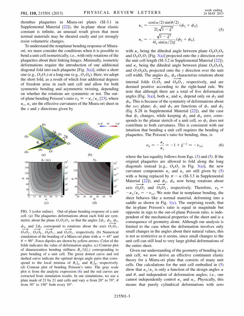
To understand the nonplanar bending response of Miura-ori, we must consider the conditions when it is possible tobend a unit cell isometrically, i.e., with only rotations of theplaquettes about their linking hinges. Minimally, isometricdeformations require the introduction of one additionaldiagonal fold into each plaquette [Fig. 3(a)], either a shortone (e.g.,O2O7) or a long one (e.g.,O1O8). Here, we adoptthe short fold, as a result of which four additional degreesof freedom arise in each unit cell and allow for bothsymmetric bending and asymmetric twisting, dependingon whether the rotations are symmetric or not. The out-of-plane bending Poisson’s ratio b y=x [23], where

x, y are the effective curvatures of the Miura-ori sheet in

the x and y directions given by

x ¼ cosð=2Þ sinð=2Þ2le

ffiffiffiffiffiffiffiffiffiffiffiffiffiffi1 2

p ð2 þ4Þ;

y ¼ ffiffiffiffiffiffiffiffiffiffiffiffiffiffi1 2

p4le sinð=2Þ ð2 þ4Þ;

(5)

with x being the dihedral angle between plane O6O3O9

andO4O1O7 [Fig. 3(a)] projected onto the x direction overthe unit cell length (SI-3.2 in Supplemental Material [22]),and y being the dihedral angle between plane O4O5O6

and O7O8O9 projected onto the y direction over the unitcell width. The angles 2, 4 characterize rotations about

internal folds O7O2

!and O8O3

!, respectively, and are

deemed positive according to the right-hand rule. Wenote that although there are a total of five deformationangles [Fig. 3(a)], both x and y depend only on 2 and

4. This is because of the symmetry of deformations aboutthe xoz plane; 3 and 5 are functions of 1 and 2

(Eq. S.28 in Supplemental Material [22]), and the casethat 1 changes, while keeping 2 and 4 zero, corre-sponds to the planar stretch of a unit cell, so 1 does notcontribute to both curvatures. This is consistent with ourintuition that bending a unit cell requires the bending ofplaquettes. The Poisson’s ratio for bending, thus, is

b ¼ y

x

¼ 1þ 2 ¼ wl; (6)

where the last equality follows from Eqs. (3) and (5). If theoriginal plaquettes are allowed to fold along the longdiagonals instead [e.g., O8O1 in Fig. 3(a)], the newcurvature components x and y are still given by (5)

with being replaced by (SI-3.3 in SupplementalMaterial [22]), and 2, 4 now being rotations about

axis O8O1

!and O9O2

!, respectively. Therefore, b ¼

y=x ¼ wl. We note that in nonplanar bending, the

sheet behaves like a normal material, deforming into asaddle as shown in Fig. 1(c). The surprising result, thatthe in-plane Poisson’s ratio is equal in magnitude butopposite in sign to the out-of-plane Poisson ratio, is inde-pendent of the mechanical properties of the sheet and is aconsequence of geometry alone. Although our analysis islimited to the case when the deformation involves onlysmall changes in the angles about their natural values, thisis not as restrictive as it seems, since small changes to theunit cell can still lead to very large global deformations ofthe entire sheet.Given our understanding of the geometry of bending in a

unit cell, we now derive an effective continuum elastictheory for a Miura-ori plate that consists of many unitcells. Our calculations for the unit cell embodied in (5)show that x=y is only a function of the design angles

and , and independent of deformation angles; i.e., onecannot independently control x and y. Physically, this

means that purely cylindrical deformations with zero

φ

φ

φ

φ

φ

0

FIG. 3 (color online). Out-of-plane bending response of a unitcell. (a) The plaquettes deformations about each fold are sym-metric about the plane O1O2O3, so that the angles 21, 2, 3,

4, and 25 correspond to rotations about the axes O1O2

!,

O7O2

!, O2O8

!, O8O3

!, and O3O2

!, respectively. (b) Numerical

simulation of the bending of a Miura-ori plate with ¼ 45 and ¼ 90. Force dipoles are shown by yellow arrows. Color of thefolds indicates the value of deformation angles. (c) Contour plotof dimensionless bending stiffness Bx=ðkleÞ corresponding topure bending of a unit cell. The green dotted curve and reddashed curve indicate the optimal design angle pairs that corre-spond to the local minima of Bxj and Bxj, respectively.(d) Contour plot of bending Poisson’s ratio. The gray scaleplot is from the analytic expression (6) and the red curves areextracted from simulation results. In our simulations, we use aplate made of 21 by 21 unit cells and vary from 20 to 70, from 30 to 150 both every 10.

PRL 110, 215501 (2013) P HY S I CA L R EV I EW LE T T E R Sweek ending24 MAY 2013

215501-3

Gaussian curvature are impossible, as locally the unit cellcan only be bent into a saddle with negative Gaussiancurvature. In the continuum limit, this implies that theeffective stiffness matrix [24] of a two-dimensionalMiura-ori plate is singular, and has rank one. Thus, thetwo-dimensional deformations of a Miura plate can bedescribed completely by a one-dimensional beam theory.

To calculate the bending stiffness per unit width of asingle cell in the x direction Bx, we note that the elasticenergy is physically stored in the eight discrete folds[Fig. 3(a)] and thus, is expressed as kleð22

1þ23þ22

5Þþ2kplesinð=2Þð2

4þ22Þ, where k and kp are the spring

constants of the ridges and the diagonal folds of plaquettes,respectively. In an effective continuum theory, the energyassociated with the deformations of the unit cell when bentinto a sheet may be described in terms of its curvatures.Thus, associated with the curvature x, the energy per unitarea of the sheet is ð1=2ÞBxwl

2x, where the effective

bending stiffness Bx is derived by equating the discreteand continuous versions of the energy and inserting w, lfrom (1) and x from (5). In general, Bx depends onmultiple independent deformation angles, but we start bystudying the ‘‘pure bending’’ case, where a row of unitcells aligned in the x direction undergo the same deforma-tion and stretching is constrained, i.e., 1 ¼ 0 for allcells so that 2 ¼ 4. In this well-defined limit,3 ¼ ð1=2Þ2 cscð=2Þ½1 2 cos=ð1 2Þ and 5 ¼ð1=2Þ2 cscð=2Þ, so that

Bxð; Þ ¼ kle

2þ 16

kpksin3

2þ

1 2 cos

1 2

2

cot

2

ð1 2Þ3=222 cos sin cosð=2Þ : (7)

The bending stiffness per unit width of a single cell in the ydirection By is related to Bx via the expression for bending

Poisson’s ratio 2b ¼ Bx=By, where b is defined in (6). Just

as there are optimum design parameters that allow us toextremize the in-plane rigidities, we can also find theoptimal design angle pairs that minimize Bx, by setting@Bxj ¼ 0 and @Bxj ¼ 0. This gives us two curvesmðÞ and mðÞ shown in Fig. 3(c), where we haveassumed k ¼ kp. To understand the bounds on Bx, we

expand (7) in the vicinity of the extreme values of thedesign variables and and find that Bxj!0 3,Bxj!=2 ð=2 Þ1, and Bxj!0 3. We see

that Bxj! is bounded except when ð; Þ ¼ ð=2; Þ,corresponding to the case of an almost flat, unfoldedorthogonal Miura sheet. Given the geometric relationbetween Bx and By, we note that optimizing By is tanta-

mount to extremizing Bx.The deformation response of a complete Miura-ori plate

requires a numerical approach because it is impossible toassemble an entire bent plate by periodically aligning unitcells with identical bending deformations in both the x and y

directions. Our numerical model takes the form of a simpletriangular-element based discretization of the sheet, inwhich each edge is treated as a linear spring with stiffnessinversely proportional to its rest length. Each pair of adja-cent triangles is assigned an elastic hinge with a bendingenergy quadratic in its deviation from an initial rest anglethat is chosen to reflect the natural shape of the Miura-oriplate. We compute the elastic stretching forces and bendingtorques in a deformed mesh [25,26], assigning a scaledstretching stiffness that is six orders of magnitude largerthan the bending stiffness of the adjacent facets, so that wemay deform the mesh nearly isometrically. When our nu-merical model of a Miura-ori plate is bent by applied forcedipoles along its left-right boundaries, it deforms into asaddle [Fig. 3(b)]. In this state, asymmetric inhomogeneoustwisting arises inmost unit cells; indeed this is the reason forthe failure of averaging for this problem, since different unitcells deform differently, and we cannot derive an effectivetheory by considering just the unit cell. This is in contrastwith the in-plane case, where the deformations of the unitcell are affinely related to those of the entire plate. Ourresults also show that themaximal stresses typically arise inthe middle of the Miura-ori plate, away from boundaries.Thus, in a real plate, the vertices and hinges near the centerare likely to fail first unless they are reinforced.We now compare our predictions for the bending

Poisson’s ratio b of the one-dimensional beam theorywith those determined using full two-dimensional simula-tions. In Fig. 3(d), we plot b from (6) (the gray scalecontour plot) based on a unit cell and b extracted at thecenter of the bent Miura-ori plate from simulations (the redcurves). In the center of the plate where only symmetricbending and in-plane stretching modes are activated, thetwo approaches agree, but away from the center where thissymmetry is violated, this is no longer true.Folded structures, mechanical metamaterials might be

named Orikozo, from the Japanese for folded matter. Ouranalysis of the simplest of these structures is rooted in thegeometry of the unit cell as characterized by a pair of designangles and together with the constraint of piecewiseisometric deformations. We have found simple expressionsfor the linearized planar stretching rigidities Kx, Ky, and

nonplanar bending rigidities Bx and By, and shown that the

bending response of a plate can be described in terms of thatof a one-dimensional beam. Furthermore, we find that the in-planePoisson’s ratiowl < 0,while the out-of-planebendingPoisson ration b > 0, an unusual combination that is notseen in simple materials, satisfying the general relationwl ¼ l, a consequence of geometry alone. Our analysisalso allows us to pose and solve a series of design problems tofind the optimal geometric parameters of the unit cell thatlead to extrema of stretching and bending rigidities aswell ascontraction or expansion ratios of the system. This paves theway for the use of optimally designed Miura-ori patterns inthree-dimensional nanostructure fabrication [27], and raises

PRL 110, 215501 (2013) P HY S I CA L R EV I EW LE T T E R Sweek ending24 MAY 2013

215501-4

the possibility of optimal control of actuated origami-basedmaterials in soft robotics [28] and elsewhere using the simplegeometrical mechanics approaches introduced here.

We thank the Wood lab for help with laser cutting theMiura-ori plates, the Wyss Institute and the Kavli Institutefor support, and Tadashi Tokieda for discussions and thenomenclature Orikozo for these materials.

Note added in proof.—While our paper was underreview, an experimental engineering study on foldablestructures was published [29] consistent with our compre-hensive theoretical and computational approach to thegeometry and mechanics of Miura-ori.

*lm@seas.harvard.edu[1] D. R. Smith, J. B. Pendry, and M.C. Wiltshire, Science

305, 788 (2004).[2] G. N. Greaves, A. L. Greer, R. S. Lakes, and T. Rouxel,

Nat. Mater. 10, 823 (2011).[3] Wm. T.M. Forbes, Psyche 31, 254 (1924).[4] H. Kobayashi, B. Kresling, and J. F. V. Vincent, Proc. R.

Soc. B 265, 147 (1998).[5] H. Kobayashi, M. Daimaruya, and H. Fujita, Solid Mech.

Its Appl. 106, 207 (2003).[6] K. Miura, in Proceedings of 31st Congress International

Astronautical Federation, Tokyo, 1980, IAF-80-A 31:1-10.[7] E. A. Elsayed and B. B. Basily, Int. J. Mater. Prod.

Technol. 21, 217 (2004).[8] R. S. Lakes, Science 235, 1038 (1987).[9] B. D. Caddock and K. E. Evans, J. Phys. D 22, 1877

(1989); K. E. Evans and B.D. Caddock, J. Phys. D 22,1883 (1989).

[10] A. Y. Haeri, D. J. Weidner, and J. B. Parise, Science 257,650 (1992).

[11] A. L. Goodwin, D.A. Keen, and G. Tucker, Proc. Natl.Acad. Sci. U.S.A. 105, 18 708 (2008).

[12] K. E. Evans, M.A. Nkansah, J. Hutchinson, and S. C.Rogers, Nature (London) 353, 124 (1991).

[13] R. Lang, Origami Design Secrets: Mathematical Methodsfor an Ancient Art (A K Peters/CRC Press, Boca Raton,FL, 2011), 2nd ed.

[14] E. Demaine and J. O’Rourke, Geometric FoldingAlgorithms: Linkages, Origami, Polyhedra (CambridgeUniversity Press, Cambridge, England, 2007).

[15] T. Hull, Project Origami: Activities for ExploringMathematics (A K Peters/CRC Press, Boca Raton, FL,2011).

[16] Y. Klettand and K. Drechsler, in Origami5: InternationalMeeting of Origami, Science, Mathematics, andEducation, edited by P. Wang-Iverson, R. J. Lang, andM. Yim (CRC Press, Boca Raton, FL, 2011), pp. 305–322.

[17] M. Schenk and S. Guest, in Origami5: InternationalMeeting of Origami, Science, Mathematics, andEducation, edited by P. Wang-Iverson, R. J. Lang, andM. Yim (CRC Press, Boca Raton, FL, 2011), pp. 291–304.

[18] A. Papa and S. Pellegrino, J. Spacecr. Rockets 45, 10(2008).

[19] N. Bowden, S. Brittain, A. G. Evans, J.W. Hutchinson,and G.M. Whitesides, Nature (London) 393, 146(1998).

[20] L. Mahadevan and S. Rica, Science 307, 1740 (2005).[21] B. Audoly and A. Boudaoud, J. Mech. Phys. Solids 56,

2444 (2008).[22] See Supplemental Material at http://link.aps.org/

supplemental/10.1103/PhysRevLett.110.215501 fordetailed derivations.

[23] In general, the incremental Poisson’s ratio is b ¼dy=dx, but here, we only consider linear deformationsabout the flat state, so b ¼ y=x.

[24] E. Ventsel and T. Krauthammer, Thin Plates and Shells:Theory, Analysis, and Applications (CRC Press, BocaRaton, FL, 2001), 1st ed., pp. 197–199.

[25] R. Bridson, S. Marino, and R. Fedkiw, ACM SIGGRAPH/Eurograph. Symp. Comp. Animation (SCA) (2003),pp. 28–36.

[26] R. Burgoon, E. Grinspun, and Z. Wood, in Proceedings ofthe ISCA 21st International Conference on Computers andTheir Applications, (ISCA, 2006), p. 180.

[27] W. J. Arora, A. J. Nichol, H. I. Smith, and G. Barbastathis,Appl. Phys. Lett. 88, 053108 (2006).

[28] E. Hawkes, B. An, N. Benbernou, H. Tanaka, S. Kim,E. D. Demaine, D. Rus, and R. J. Wood, Proc. Natl. Acad.Sci. U.S.A. 107, 12 441 (2010).

[29] M. Schenk and S. Guest, Proc. Natl. Acad. Sci. U.S.A.110, 3276 (2013).

PRL 110, 215501 (2013) P HY S I CA L R EV I EW LE T T E R Sweek ending24 MAY 2013

215501-5

Supplementary Material for“Geometric Mechanics of Periodic Pleated

Origami” by Wei et al.

March 23, 2013

Contents

1 Geometry and Kinematics 1

2 In-plane stretching response of a Miura-ori plate 42.1 Poisson’s ratio related to height changes . . . . . . . . . . . . . . . . . . . . . . . . . 42.2 Stretching stiffness Kx and Ky . . . . . . . . . . . . . . . . . . . . . . . . . . . . . . 42.3 Asymptotic cases for optimal design angles . . . . . . . . . . . . . . . . . . . . . . . 5

3 Out-of-plane bending response of a Miura-ori plate 63.1 Minimum model for isometric bending . . . . . . . . . . . . . . . . . . . . . . . . . . 63.2 Curvatures and the bending Poisson’s ratio when short folds are introduced . . . . . 73.3 Curvatures and the bending Poisson’s ratio when long folds are introduced . . . . . 103.4 Bending stiffness Bx and By . . . . . . . . . . . . . . . . . . . . . . . . . . . . . . . . 113.5 Pure bending . . . . . . . . . . . . . . . . . . . . . . . . . . . . . . . . . . . . . . . . 12

4 Numerical simulations of the bending response of a Miura-ori plate 124.1 Homogeneous deformation in bent plate is impossible . . . . . . . . . . . . . . . . . . 124.2 Simulation model . . . . . . . . . . . . . . . . . . . . . . . . . . . . . . . . . . . . . . 12

1 Geometry and Kinematics

The unit cell of a Miura-ori patterned plate is shown in Fig.S.1 and is parameterized by two dihedralangles θ ∈ [0, π], β ∈ [0, π], and one oblique angle α, in a unit cell of length l, width w, and heighth. We treat the structure as being made of identical periodic rigid skew plaquettes joined by elastichinges at the ridges. The structure can deploy uniformly in the plane by having each constituentskew plaquette in a unit cell rotate rigidly about the connecting elastic ridges. Then the ridgelengths l1, l2 and α ∈ [0, π/2] are constant through folding/unfolding, so that we may choose θ(or equivalently β) to be the only degree of freedom that completely characterizes a Miura-ori cell.

1

θ

β

hl2

l1l2

l1

l

wα

O6O2

O5

O4

O1

O7

O8

O9

O3

Figure S.1: Sketch of a unit cell of Miura Ori pattern.

The geometry of the unit cell implies that

β = 2 sin−1(ζ sin(θ/2)), l = 2l1ζ,

w = 2l2ξ and h = l1ζ tanα cos(θ/2),(S.1)

where the dimensionless width and height are

ξ = sinα sin(θ/2) and ζ = cosα(1− ξ2)−1/2. (S.2)

We see that β, l, w, and h change monotonically as θ ∈ [0, π], with β ∈ [0, π], l ∈ 2l1[cosα, 1],w ∈ 2l2[0, sinα], and h ∈ l1[sinα, 0]. As α ∈ [0, π/2], we see that β ∈ [θ, 0], l ∈ [2l1, 0], w ∈[0, 2l2 sin(θ/2)] and h ∈ [0, l1].

Before we discuss the coupled deformations of the plate embodied functionally as β(α, θ), weinvestigate the case when α = π/2 corresponding to an orthogonally folded map that can onlybe completely unfolded first in one direction and then another, without bending or stretching thesheet except along the hinges. Indeed, when α = π/2 and θ 6= π, Eq. (S.1) reduces to β = 0,l = 0 and h = l1, the singular limit when Miura-ori patterned sheets can not be unfolded witha single diagonal pull. Close to this limiting case, when the folds are almost orthogonal, theMiura-ori pattern can remain almost completely folded in the x direction (β changes only by asmall amount) while unfolds in the y direction as θ is varied over a large range, only to expandsuddenly in the x direction at the last moment. This observation can be explained by expandingEq. (S.1) asymptotically as α → π/2 and θ → π, which yields β ≈ π − ε/δ, l ≈ l1(2 − (ε/δ)2/4),w ≈ l2(2 − δ2 − ε2/4) and h ≈ l1ε/(2δ), where δ = π/2 − α and ε = π − θ. Thus, we see that forany fixed small constant δ, only when ε < δ, do we find that β → π, l → 2l2 and h → 0, leadingto a sharp transition in the narrow neighborhood (∼ δ) of θ = π as α→ π/2 (Fig.S.2a), consistentwith our observations.

More generally, we start by considering the volumetric packing of Miura-ori characterized bythe effective volume of a unit cell V ≡ l × w × h = 2l21l2ζ

2 sin θ sinα tanα, which vanishes whenθ = 0, π. To determine the conditions when the volume is at an extremum for a fixed in-planeangle α, we set ∂θV |α = 0 and find that the maximum volume

Vmax|α = 2l21l2 sin2 α at θm = cos−1(

cos 2α− 1

cos 2α+ 3

), (S.3)

2

(a) (b)

0 15 30 45 60 75 900

30

60

90

120

150

180

0

0.2

0.4

0.6

0.8

1θ

β ⁄

α

V/(2l l )1 2

2

0 15 30 45 60 75 900

30

60

90

120

150

180

0

0.2

0.4

0.6

0.8

1

θ

α(c)

K / ky

0 15 30 45 60 75 900

30

60

90

120

150

180

10

10

10

10

10

103

2.5

2

1.5

1

0.5

α

θ 0

Figure S.2: Geometry of the unit cell as a function of α and θ. (a) The folding angle β increasesas θ increases and decreases as α increases. The transition becomes sharper as α ≈ π/2, and whenα = π/2, β = 0 independent of θ, i.e. the unfolding (folding) of folded (unfolded) of maps with Northogonal folds has 2N decoupled possibilities. (b) Effective dimensionless volume V/(2l21l2). Thegreen dotted curve θm(α) indicates the optimal design angle pairs that correspond to the maximumV |α. The red dashed curve αm(θ) indicates the optimal design angle pairs that correspond to themaximum V |θ. (c) Contour plot of the dimensionless stretching rigidity Ky/k. Ky|α is monotonicin θ0. The green dotted curve indicates the design angle pairs that correspond to the minima ofKy|θ0 . The red dashed curve indicates the design angle pairs that correspond to the maxima ofKx|θ0 . See the text for details.

shown as a red dashed line in Fig.S.2b. Similarly, for a given dihedral angle θ, we may ask when thevolume is extremized as a function of α? Using the condition ∂αV |θ = 0 shows that the maximumvolume is given by

Vmax|θ =4l21l2 cosαm

(√5 + 4 cos θ − 3

)cot2 (θ/2) sin θ

√5 + 4 cos θ − 3− 2 cos θ

(S.4)

at

αm = cos−1

[√(2 + cos θ −

√5 + 4 cos θ

)/(cos θ − 1)

],

shown as a red dashed line in Fig.S.2b. These relations for the maximum volume as a function ofthe two angles that characterize the Miura-ori allow us to manipulate the configurations for thelowest density in such applications as packaging for the best protection. In the following sections,we assume each plaquette is a rhombus, i.e. l1 = l2 = le, to keep the size of the algebraic expressionsmanageable, although it is a relatively straightforward matter to account for variations from thislimit.

3

2 In-plane stretching response of a Miura-ori plate

2.1 Poisson’s ratio related to height changes

Poisson’s ratios related to height changes, νhl

and νwl

read

νhl

= ν−1lh≡ −dh/h

dl/l= cot2 α sec2

θ

2,

νhw

= ν−1wh≡ − dh/h

dw/w= ζ2 tan2 θ

2.

(S.5)

which are both positive, and monotonically increasing with θ and α. Expansion of νhl

in Eq.(S.5) shows that ν

hl|θ→π ∼ (π − θ)−2 and thus ν

hl|α ∈ [cot2 α,∞), while ν

hl|α→0 ∼ α−2 and thus

νhl|θ ∈ (∞, 0]. Similarly, expansion of ν

hwin Eq. (S.5) shows that ν

hw|θ→π ∼ (π − θ)−2 and

thus νhw|α ∈ [0,∞), while ν

hw|θ ∈ [tan2(θ/2), 0]. Finally, it is worth pointing out that ν

hwhas a

singularity at (α, θ) = (π/2, π).

2.2 Stretching stiffness Kx and Ky

Here we derive the expressions for stretching stiffness Kx and Ky.The expression for the potential energy of a unit cell deformed by a uniaxial force fx in the x

direction is given by

H = U −∫ θ

θ0

fxdl

dθ′dθ′, (S.6)

where the unit cell length l is defined in Eq. (S.1). The elastic energy of a unit cell U is storedonly in the elastic hinges which allow the plaquettes to rotate, and is given by

U = kle(θ − θ0)2 + kle(β − β0)2, (S.7)

where k is the hinge spring constant, and θ0 and β0 (= β(α, θ0)) are the natural dihedral angles inthe undeformed state. The external force fx at equilibrium state is obtained using the conditionthat the first variation δH/δθ = 0, which reads

fx =dU/dθ

dl/dθ= 2k

(θ − θ0) + (β − β0)$(α, θ)

η(α, θ), (S.8)

where U is defined in Eq. (S.7), l is defined in Eq. (S.1), and in addition

$(α, θ) =cosα

1− ξ2and η(α, θ) =

cosα sin2 α sin θ

2(1− ξ2)3/2. (S.9)

The stretching rigidity associated with the x direction is thus given by

Kx(α, θ0) ≡dfxdθ

∣∣∣∣θ0

= 4k(1− ξ20)2 + cos2 α

(1− ξ20)12 cosα sin2 α sin θ0

, (S.10)

where ξ0 = ξ(α, θ0).

4

Similarly, the uniaxial force in the y direction in a unit cell at equilibrium is

fy =dU/dθ

dw/dθ= 2k

(θ − θ0) + (β − β0)$(α, θ)

sinα cos(θ/2), (S.11)

where w is defined in Eq. (S.1) and $ is defined in Eq. (S.9). The stretching rigidity in y directionis thus given by

Ky(α, θ0) ≡dfydθ

∣∣∣∣θ0

= 2k(1− ξ20)2 + cos2 α

(1− ξ20)2 sinα cos(θ0/2), (S.12)

of which the contour plot is show in Fig. S.2c.

2.3 Asymptotic cases for optimal design angles

The expressions in Section 2.2 allow us to derive in detail all the asymptotic cases associated withthe optimal pairs of design angles which correspond to the extrema of stretching rigidities Kx andKy. For simplicity, we use (α, θ) instead of (α, θ0) to represent the design angle pairs when the unitcell is at rest.

1. Expanding ∂θKx in the neighborhood of α = 0 yields

∂θKx|α→0 = −8 cot θ csc θ

α2− 2

3

((3 + cos θ) csc2 θ

)+O(α2). (S.13)

As α → 0, θ → π/2 to prevent a divergence. Continuing to expand Eq. (S.13) in theneighborhood of θ = π/2 and keeping the first two terms yields

∂θKx|θ→π/2 = 0⇒ 4(θ − π/2) = α2. (S.14)

Therefore in the contour plot of Kx (Fig.3b in the main text), the greed dotted curve isapproximated by 4(θ − π/2) = α2 in the neighborhood of α = 0, and is perpendicular toα = 0 as θ is quadratic in α.

2. Expanding ∂αKx in the neighborhood of θ = 0 yields

∂αKx|θ→0 =− [11 + 20 cos(2α) + cos(4α)] csc3 α sec2 α

2θ− 1

192[290 + 173 cos(2α)

+46 cos(4α) + 3 cos(6α)] csc3 α sec2 αθ +O(θ2).

(S.15)

The numerator of the leading order in Eq. (S.15) has to vanish as θ → 0 to keep the result

finite, which results in a unique solution α∗ = cos−1(√√

5− 2)

in the domain α ∈ (0, π/2).

Continuing to expand Eq. (S.15) in the neighborhood of α = α∗ and only keeping the firsttwo terms yields

∂αKx = 0|α→α∗ ⇒ 4

√5(1 +

√5)(α− α∗) = θ2. (S.16)

so the red dashed curve in the contour plot of Kx (Fig.3b in the main text) is perpendicularto θ = 0.

5

3. Similarly, Expansion of ∂αKy near θ = π yields

∂αKy|θ→π =[−1 + 16 cos(2α) + cos(4α)] csc2 α sec3 α

2(θ − π)+

1

192[638− 737 cos(2α)+

162 cos(4α) + cos(6α)] csc2 α sec5 α(θ − π) +O[(θ − π)3].

(S.17)

Allowing for a well behaved limit at leading order as θ → π requires−1+16 cos(2α)+cos(4α) =

0 and yields α∗ = cos−1(√

(√

17− 3)/2

)as the unique solution when α is an acute. Again

expanding Eq. (S.17) in the neighborhood of θ = π, and only keeping the first two termsyields

∂αKy|α→α∗ = 0⇒ 2

√1 +√

17(αm − α∗) = (π − θ)2. (S.18)

So the green dotted curve in the contour plot ofKy (Fig. S.2c) is approximated by 2√

1 +√

17(αm−α∗) = (π − θ)2 near α = α∗, and is perpendicular to θ = π. The point where the green curveends satisfies the condition

∂αKy = 0 and ∂α (∂αKy) = 0 (S.19)

and numerical calculation gives us the coordinates of this critical point as

θ = 2.39509, and α = 1.00626. (S.20)

The red dashed curve (Fig. S.2c) starting at this point shows a collection of optimal designangle pairs (α, θ) where Ky|θ is locally maximal.

3 Out-of-plane bending response of a Miura-ori plate

3.1 Minimum model for isometric bending

Here we show that planar folding is the only geometrically possible motion under the assumptionthat the unit cell deforms isometrically, i.e. with only rotations of the rhombus plaquettes about thehinges. To enable the out-of-plane bending mode, the minimum model for isometric deformationsrequires the introduction of 1 additional diagonal fold into each plaquette, and this follows fromthe explanation below.

Suppose the plane O1O2O5O4 (Fig.S.3a) is fixed to eliminate all rigid motions, for any dihe-dral angle θ, the orientation of plane O1O2O8O7 is determined. However, the other two rhombiO2O5O6O3 and O2O3O9O8 are free to rotate about axis O2O5 and O2O8 respectively and sweepout two cones which intersect at O2O3 and O2O

′3. Fig.S.3a shows the two possible configurations of

a unit cell determined from the two intersections, the yellow part being the red part that has beenflipped about a plane of symmetry. The unit cell in red is the only nontrivial Miura pattern, so thatfor any given θ, there is a unique configuration of the unit cell corresponding to it. Any continuouschange in θ results in the unit cell being expanded or folded but remaining planar, in which case,O1, O4, O7, O3, O6 and O9 also remain coplanar. In order to enable the bending mode of the unitcell, the planarity of each plaquette must be violated. In the limit where the plaquette thicknesst 1 the stretching rigidity (∼ t) is much larger than the bending rigidity (∼ t3), with t beingthe thickness of a plaquette, while the energy required to bend a strip of ridge is 5 times of that

6

o1

o2

o3

o4

o5

o6

o7

o8

o9

(b) (c)

φ2

2φ1φ

3

2φ5

φ4

o1

o2

o3o4

o5

o6

o8

o9

o3’’

’

o6

o9

(a)o7

Figure S.3: Bending of a unit cell. (a) The two configurations of a unit cell for any given θ ifeach plaquette is a rigid rhombus. The only possible motion is in-plane stretching. The yellowplaquettes illustrate the trivial configuration of two rigid plaquettes and the red ones show thetypical configuration of a Miura-ori unit cell. (b) The undeformed state. An additional fold alongthe short diagonal is introduced to divide each rhombus into 2 elastically hinged triangles. (c)

Symmetrically bent state. The bending angles around axis−−−→O2O4 and

−−−→O3O5 are the same as those

around−−−→O7O2 and

−−−→O8O3 respectively.

required to stretch it according to the asymptotic analysis of the F oppl − von Karman equations[1]. Therefore, the rigid ridge/fold is an excellent approximation for out-of-plane bending whent 1. Then, to get a bent shape in a unit cell and thence in a Miura-ori plate, we must introducean additional fold into each rhombus to divide it into two elastically hinged triangles (Fig.S.3b).As a result, 4 additional degrees of freedom are introduced in each unit cell. The deformed statecan either be symmetrical about the plane O1O2O3 (Fig.S.3c) corresponding to a bending mode,or unsymmetrical corresponding to a twisting mode. Here, we are only interested in the bent state,

in which the rotation angle φ2 about the axis−−−→O2O4, and φ4 about the axis

−−−→O3O5, are the same as

the rotations about−−−→O7O2 and

−−−→O8O3 respectively. The rotation angles about the axis

−−−→O1O2,

−−−→O3O2

and−−−→O2O5 are 2φ1, 2φ5 and φ3 respectively. (−→ indicates the direction.)

3.2 Curvatures and the bending Poisson’s ratio when short folds are introduced

Here we derive expressions for the coordinates of every vertex of the unit cell after bending in thelinear deformation regime, from which curvatures in the two principle directions κx, κy and thebending Poisson’s ratio νb = −κy/κx can be calculated.

To do so, we first need to know the transformation matrix associated with rotation about anarbitrary axis. The rotation axis is defined by a point a, b, c that it goes through and a directionvector < u, v, w >, where u, v, w are directional cosines. Suppose a point x0, y0, z0 rotates aboutthis axis by an infinitesimal small angle ω (ω 1), and reaches the new position x, y, z. Keepingonly the leading order terms of the transformation matrix, we find that the new position x, y, z

7

is given by

x = x0 + (−cv + bw − wy0 + vz0)ω,

y = y0 + (cu− aw + wx0 − uz0)ω,z = z0 + (−bu+ av − vx0 + uy0)ω.

(S.21)

Given Eq. (S.21), we are ready to calculate the coordinates of all vertices in the bent sate.Assuming that the origin is at O2, in the undeformed unit cell, edge O1O2 is fixed in xoz plane toeliminate rigid motions. Each fold deforms linearly by angle 2φ1, φ2, φ3, φ4 and 2φ5 (see Fig. S.3c)around corresponding axes respectively. The coordinates of O1 and O2 are

O1x =cosα√1− ξ2

, O1y = 0, O1z = −sinα cos(θ/2)√1− ξ2

;

O2x = 0, O2y = 0, O2z = 0.

(S.22)

The coordinates of O3 after bending are

O3x =− cosα√1− sin2 α sin2(θ/2)

− cos(α/2) sinα sin θ√3− cos(2α)(cos θ − 1) + cos θ

φ2 +sin2 α sin θ

2√

1− sin2 α sin2(θ/2)φ3,

O3y =− 4 cos(θ/2) sin(2α)

3 + cos(2α) + 2 cos θ sin2 αφ1 +

csc(θ/2)[− sinα+ sin(2α) + sin3 α sin2(θ/2)] sin θ

[3 + cos(2α) + 2 cos(θ) sin2 α] sin(α/2)φ2

+ cos(θ/2) sin(α)φ3,

O3z =− cos(θ/2) sinα√1− sin2 α sin2(θ/2)

+2 cosα cos(α/2) sin(θ/2)√

3− cos(2α)(cos θ − 1) + cos θφ2 −

cosα sinα sin(θ/2)√1− sin2 α sin2(θ/2)

φ3.

(S.23)

The coordinates of O4 after bending are

O4x =cosα+ sin2 α sin2(θ/2)− 1√

1− sin2 α sin2(θ/2)− sin2 α sin θ√

3− cos(2α)(cos θ − 1) + cos θφ1,

O4y = sinα sin(θ/2)− cos(θ/2) sinαφ1,

O4z =− cos(θ/2) sinα√1− sin2 α sin2(θ/2)

− 2 cosα sinα sin(θ/2)√3− cos(2α)(cos θ − 1) + cos θ

φ1.

(S.24)

The coordinates of O5 after bending are

O5x =−√

1− sin2 α sin2(θ/2)− sin2 α sin θ√3− cos(2α)(cos θ − 1) + cos θ

φ1

+sin2 α sin θ

2√

3− cos(2α)(cos θ − 1) + cos θ sin(α/2)φ2,

O5y = sinα sin(θ/2)− cos(θ/2) sinαφ1 +cos(θ/2) sinα

2 sin(α/2)φ2,

O5z =− 2 cosα sinα sin(θ/2)√3− cos(2α)(cos θ − 1) + cos θ

φ1 +cosα sinα sin(θ/2)√

3− cos(2α)(cos θ − 1) + cos θ sin(α/2)φ2.

(S.25)

8

The coordinates of O6 after bending are

O6x =sin2 α sin2(θ/2)− cosα− 1√

1− sin2 α sin2(θ/2)− sin2 α sin θ√

3− cos(2α)(cos θ − 1) + cos θφ1

+sin2 α sin θ

2√

1− sin2 α sin2(θ/2)φ3 −

sinα sin θ cos(α/2)√3− cos(2α)(cos θ − 1) + cos θ

φ4,

O6y = sinα sin(θ/2) +4 cos(θ/2) sinα[sin2 α sin2(θ/2)− 1− 2 cosα]

3 + cos(2α) + 2 cos θ sin2 αφ1

+8 cosα cos(θ/2) cos(α/2)

3 + cos(2α) + 2 cos θ sin2 αφ2 + cos(θ/2) sinαφ3 − cos(θ/2) cos(α/2)φ4,

O6z =− cos(θ/2) sinα√1− sin2 α sin2(θ/2)

− 2 cosα sinα sin(θ/2)√3− cos(2α)(cos θ − 1) + cos θ

φ1

+csc(α/2) sin(2α) sin(θ/2)√

3− cos(2α)(cos θ − 1) + cos θφ2 −

cosα sinα sin(θ/2)√1− sin2 α sin2(θ/2)

φ3

+2 cosα cos(α/2) sin(θ/2)√

3− cos(2α)(cos θ − 1) + cos θφ4.

(S.26)

The coordinates of O7, O8 and O9 after bending are

O7x, O7y, O7z = O4x,−O4y, O4z, O8x, O8y, O8z = O5x,−O5y, O5z,O9x, O9y, O9z = O6x,−O6y, O6z.

(S.27)

Due to symmetry, O3 must lie in the xoz plane after bending, so O3y = 0, from which φ3 andφ5 can be expressed as a function of φ1 and φ2,

φ3 =8 cosα

3 + cos(2α) + 2cosθ sin2 αφ1 +

1

2csc(α

2

)(1− 8 cosα

3 + cos(2α) + 2 cos θ sin2 α

)φ2.

φ5 = φ1 −1

2csc(α

2

)φ2

(S.28)

The curvature of the unit cell in the x direction is defined as the dihedral angle formed byrotating plane O4O1O7 to plane O6O3O9 projected onto the x direction over the unit length l. Thesign of the angle follows the right-hand rule about the y axis. The dihedral angle between planeO4O1O7 and plane xoy is

Ω417 =O4z −O1z√

1− ξ2= − 4 cosα sinα sin(θ/2)

3 + cos(2α) + 2 cos θ sin2 αφ1, (S.29)

and the dihedral angle between plane O3O6O9 and plane xoy is

Ω639 =O6z −O3z√

1− ξ2=

2[cos(α/2) + cos(3α/2)][φ2 + φ4 − 2φ1 sin(α/2)] sin(θ/2)

3 + cos(2α) + 2 cos θ sin2 α. (S.30)

The curvature κx hence is

κx =Ω639 − Ω417

l=

(φ2 + φ4) cos(α/2) sin(θ/2)

2√

1− ξ2. (S.31)

9

The curvature of the unit cell in the y direction is defined as the dihedral angle between planeO4O5O6 and O7O8O9 projected onto the y direction over the unit cell width w, which is expressedas

κy = −2O5y −O4y −O3y

hw= −1

4(φ2 + φ4) csc

(α2

)cscα csc

(θ

2

)√1− ξ2. (S.32)

From Eq. (S.31) and Eq. (S.32), we can calculate the bending Poisson ratio, which is simplifiedto

νb = −κyκx

= −1 + csc2 α csc2(θ

2

). (S.33)

3.3 Curvatures and the bending Poisson’s ratio when long folds are introduced

In Fig.S.3, if we introduce the additional fold along the long diagonal, e.g. O1O5, instead of theshort one, the unit cell can be bent too. In this case, φ2 and φ4 are bending angles around axis−−−→O1O5 and

−−−→O2O6 respectively. O1, O2 do not change as they are fixed, and coordinates of O3 after

bending are

O3x =− cosα√1− sin2 α sin2(θ/2)

+sin2 α sin θ

2√

1− sin2 α sin2(θ/2)φ3 −

sinα sin(α/2) sin θ√3− cos(2α)(cos θ − 1) + cos θ

φ4,

O3y =− 4 cos(θ/2) sin(2α)

3 + cos(2α) + 2 cos θ sin2 αφ1 + cos

(θ

2

)sin(α)φ3 − cos

(θ

2

)sin(α

2

)φ4,

O3z =− cos(θ/2) sin(α)√1− sin2 α sin2(θ/2)

− cosα sinα sin(θ/2)√1− sin2 α sin2(θ/2)

φ3 +2 cosα sin(α/2) sin(θ/2)√

3− cos(2α)(cos θ − 1) + cos θφ4.

(S.34)

The coordinates of O4 after bending are

O4x =cosα− 1 + sin2 α sin2(θ/2)√

1− sin2 α sin2(θ/2)− sin2 α sin θ√

3− cos(2α)(cos θ − 1) + cos θ

[φ1 −

1

2sec(α

2

)φ2

],

O4y = sinα sin(θ/2)− cos(θ/2) sinαφ1 + cos(θ/2) sin(α/2)φ2,

O4z =− cos(θ/2) sinα√1− sin2 α sin2(θ/2)

− 2 cosα sin(θ/2) sin(α/2)√3− cos(2α)(cos θ − 1) + cos θ

[2 cos

(α2

)φ1 − φ2

].

(S.35)

The coordinates of O5 after bending are

O5x =−

√1− sin2 α sin2

(θ

2

)− sin2 α sin θ√

3− cos(2α)(cos θ − 1) + cos θφ1,

O5y = sinα sin(θ/2)− cos(θ/2) sinαφ1,

O5z =− sin(2α) sin(θ/2)√3− cos(2α)(cos θ − 1) + cos θ

φ1.

(S.36)

10

The coordinates of O6 after bending are

O6x =sin2 α sin2(θ/2)− cosα− 1√

1− sin2 α sin2(θ/2)− sin2 α sin θ√

3− cos(2α)(cos θ − 1) + cos θφ1 +

sin2 α sin θ

2√

1− sin2 α sin2(θ/2)φ3,

O6y = sinα sin

(θ

2

)+

4 cos(θ/2) sinα[−1− 2 cosα+ sin2 α sin2(θ/2)

]3 + cos(2α) + 2 cos θ sin2 α

φ1 + cos

(θ

2

)sinαφ3,

O6z =− cos(θ/2) sinα√1− sin2 α sin2(θ/2)

− sin(2α) sin(θ/2)√3− cos(2α)(cos θ − 1) + cos θ

φ1 −cosα sinα sin(θ/2)√1− sin2 α sin2(θ/2)

φ3.

(S.37)

Using the same idea for the long fold case as we did for the short fold, we can also calculate thecurvatures in the two principal directions and find that

κx =Ω639 − Ω417

l=

2 [sin(α/2)− sin(3α/2)] sin(θ/2)

[3 + cos(2α) + 2 cos θ sin2 α]l(φ2 + φ4) =

sin (α/2) sin (θ/2)

2le√

1− ξ2(φ2 + φ4),

(S.38)while

κy = −2O5y −O4y −O3y

hw= −

√1− sin2 α sin2(θ/2)

2 cos(α/2)w(φ2 + φ4) = −

√1− ξ2

4le cos (α/2) ξ(φ2 + φ4). (S.39)

Therefore the bending Poisson ratio is

νb = −κyκx

= −1 + csc2 α csc2(θ

2

), (S.40)

which is the same as that of the case when the short folds are introduced.

3.4 Bending stiffness Bx and By

We are now in a position to derive expressions for the bending stiffness Bx and By. On onehand, the bending energy is physically stored in the 8 discrete folds, which can be expressed as1/2kle[4φ

21 + 4 sin(α/2)φ22 + 2φ23 + 4 sin(α/2)φ24 + 4φ25]. On the other hand from a continuum point

of view, the energy may also be effectively considered as stored in the entire unit cell that is bentinto the curvature κx, which can be expressed as 1/2Bxwlκ

2x. Equating the two expressions for the

same energy, we can write Bx as

Bx =kle4φ21 + 4

kpk sin(α2 )φ22 + 2φ23 + 4

kpk sin(α2 )φ24 + 4φ25

wlκ2x,

=kle

[2 + 16

kpk

sin3 α

2+

(1− 2 cosα

1− ξ2

)2]

cot

(θ

2

)(1− ξ2)3/2

2ξ2 cosα sinα cos(θ/2),

(S.41)

where k is the spring constant of the fold between two adjacent plaquettes, and kp is the springconstant of the additional internal fold within a plaquette.

Just as there are optimum design parameters that allow us to extremize the in-plane rigidities,we can also find the optimal design angle pairs that lead to minima of Bx, by setting ∂θBx|α = 0and ∂αBx|θ = 0. This gives us two curves θm(α) and αm(θ) respectively shown in Fig.3 in the main

11

text. The green dotted curve θm(α) starts from (α, θ) ≈ (1.1, π), and ends at (α, θ) = (π/2, π). Itis asymptotically approximated by 2.285(α− 1.1) ≈ (π− θm)2 when α→ 1.1. The red curve θm(α)starts from (α, θ) ≈ (.913, 0), and ends at (α, θ) = (π/2, π), and is asymptotically approximated by17.752(αm − 0.913) ≈ θ2 when θ → 0.

Similarly, the bending stiffness per unit width of a single cell in the y direction is

By(α, θ) = kle4φ21 + 4

kpk sin(α2 )φ22 + 2φ23 + 4

kpk sin(α2 )φ24 + 4φ25

wlκ2y(S.42)

3.5 Pure bending

Finally, we explain the “pure bending” situation in the main text, borrowing ideas from notionsof the pure bending of a beam where curvature is constant. If we demand that a row of unitcells aligned in the x direction (e.g. the cell C1 and C2 in Fig.S.4) undergo exactly the samedeformation, this results in φ2 = φ4. Furthermore, in this limit, the stretching mode is constrained,so that φ1 = 0 for all cells. For this well defined bending deformation, the bending stiffness dependsonly on the design angles, not on the deformation angles as shown in Eq. (S.41) and Eq. (S.42).

4 Numerical simulations of the bending response of a Miura-oriplate

4.1 Homogeneous deformation in bent plate is impossible

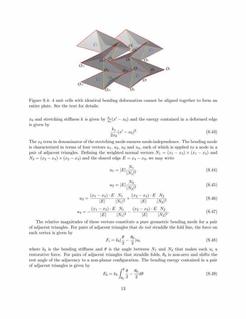
Here we explain why it is impossible to assemble an entire bent plate by periodically aligning unitcells with identical bending deformation in both the x and y direction.

In Fig.S.4, the 4 unit cells C1, C2, C3 and C4 have identical bending deformations: C1 and C2

align perfectly in the x direction, which requires that 6 O4O1O7 = 6 O6O3O9 = 6 O11O13O15. C1

and C3, C2 and C4 align perfectly in the y direction respectively, which is automatically satisfiedby the symmetry of the unit cell. Now the question becomes whether the unit cell C3 and C4 canalign together? The answer is no. The reasoning is as follows. O3 and O

′3 are symmetric about

plane O6O12O13, while O3 and O′′3 are symmetric about plane O4O5O6. However plane O6O12O13

and plane O4O5O6 are not coplanar unless all the deformation angles about the internal folds arezero, which is violated by bending. O

′3 and O

′′3 thus do not coincide. In fact O

′3 = O

′′3 if and only

if O3y = O5y = O6y, which requires φ2 = φ4 = 0 from Eq. (S.24), Eq. (S.25), Eq. (S.26) and Eq.(S.28). This is the in-plane stretching mode instead of the bending mode. In conclusion, in thebent Miura-ori plate, the deformation must be inhomogeneous.

4.2 Simulation model

In this subsection, we explain the bending model and the strategies used to bend the Miura-oriplate.

We endow these triangulated meshes with elastic stretching and bending modes to capture thein-plane and out-of-plane deformation of thin sheets. The stretching mode simply treats each edgein the mesh as a linear spring, all edges having the same stretching stiffness. Accordingly, themagnitude of the restorative elastic forces applied to each node in a deformed edge with rest length

12

O1O2O3

O4O5O6

O7O9

O8

O10O11

O12

O13

O14

O15

O3’

O3’’

C1

C2

C3

C4

Figure S.4: 4 unit cells with identical bending deformation cannot be aligned together to form anentire plate. See the text for details.

x0 and stretching stiffness k is given by ksx0

(x′ − x0) and the energy contained in a deformed edgeis given by

ks2x0

(x′ − x0)2 (S.43)

The x0 term in denominator of the stretching mode ensures mesh-independence. The bending modeis characterized in terms of four vectors u1, u2, u3 and u4, each of which is applied to a node in apair of adjacent triangles. Defining the weighted normal vectors N1 = (x1 − x3) × (x1 − x4) andN2 = (x2 − x4)× (x2 − x3) and the shared edge E = x4 − x3, we may write

u1 = |E| N1

|N1|2(S.44)

u2 = |E| N2

|N2|2(S.45)

u3 =(x1 − x4) · E

|E|N1

|N1|2+

(x2 − x4) · E|E|

N2

|N2|2(S.46)

u4 = −(x1 − x3) · E|E|

N1

|N1|2− (x2 − x2) · E

|E|N2

|N2|2. (S.47)

The relative magnitudes of these vectors constitute a pure geometric bending mode for a pairof adjacent triangles. For pairs of adjacent triangles that do not straddle the fold line, the force oneach vertex is given by

Fi = kb(θ

2− θ0

2)ui (S.48)

where kb is the bending stiffness and θ is the angle between N1 and N2 that makes each ui arestorative force. For pairs of adjacent triangles that straddle folds, θ0 is non-zero and shifts therest angle of the adjacency to a non-planar configuration. The bending energy contained in a pairof adjacent triangles is given by

Eb = kb

∫ θ

θ0

θ

2− θ0

2dθ (S.49)

13

N1 N2

u3

u1

u4

u2

x1x2

x4

x3

(a) (b)

Figure S.5: Simulation model. (a) A single bending adjacency. The vectors ui illustrate the purelygeometric bending mode and N1 and N2 are the weighted normals of the adjacent triangles. (b)The left-right bending strategy is shown in yellow and the up-down bending strategy is shown ingreen. Each arrow represents a force applied to its incident vertex. Left-right force directions bisectthe yellow adjacencies and are perpendicular to the shared edge and up-down force directions arenormal to the plane spanned by each pair of green edges.

with a precise form of

Eb = kb(θ

2− θ0

2)2 (S.50)

which is quadratic in θ for θ ∼ θ0.We introduce viscous damping so that the simulation eventually comes to rest. Damping forces

are computed at every vertex with different coefficients for each oscillatory mode, bending andstretching. We distinguish between these two modes by projecting the velocities of the verticesin an adjacency onto the bending mode, and the velocities of the vertices in an edge onto thestretching mode.

We use the Velocity Verlet numerical integration method to update the positions and velocitiesof the vertices based on the forces from the bending and stretching model and the external forcesfrom our bending strategies. At any time t + ∆t during the simulation we can approximate theposition x(t+ ∆t) and the velocity x(t+ ∆t) of a vertex as

x(t+ ∆t) = x(t) + x(t) ∆t+1

2x(t) ∆t2 (S.51)

x(t+ ∆t) = x(t) +x(t) + x(t+ ∆t)

2∆t (S.52)

A single position, velocity and accleration update follows a simple algorithm.

• Compute x(t+ ∆t)

• Compute x(t + ∆t) using x(t + ∆t) for stretching and bending forces and x(t) for dampingforces

• Compute x(t+ ∆t)

14

Figure S.6: 3D geometry of a bent Miura plate made of 21 by 21 unit cells with α = θ = π/3.For better display purpose, we use an example with pronounced deformation. However in thesimulation we have done, we make sure that the radius of curvature is at least 10 times larger thanthe plate size, such that the deformation is within linear regime. Readers may want to play withdifferent toolbar options to better visualize the geometry.

15

Note that this algorithm staggers the effects of damping on the simulation by ∆t.In simulation, the Miura-ori plate is made of 21 by 21 unit cells, 21 being the number of unit

cells in one direction. α varies from 20o to 70o, and θ varies from 30o to 150o, both every 10o. Wedesign two bending strategies, each of which corresponds to a pair of opposite boundaries. Theleft-right bending strategy identifies the adjacencies with O2O3 shared edges on left boundary unitcells and O1O2 shared edges on right boundary unit cells (highlighted in yellow in Fig.S.5b). Foreach of these adjcencies we apply equal and opposite forces to the vertices on their shared edge,the directions of which are determined to lie in the bisecting plane of O1O2O4 and O1O2O7 (leftboundary unit cells) and O2O3O5 and O2O3O8 (right boundary unit cells) and perpendicular tothe shared edge. The up-down bending strategy identifies the top edges of each unit cell on theup and down boundaries of the pattern (shown in green in Fig.S.5b). Each unit cell has one suchpair of edges and we apply equal and opposite forces to the not-shared vertices in this pair, thedirections of which are normal to the plane spanned by the pair of edges. We take out the 11throw and 11th column of vertices on the top surface as two sets of points to locally interpolate thecurvature near the center of the plate in x and y direction respectively. The largest difference of νbfor the same design angle pairs α and θ between both B.Cs applied is less than 0.5%.

By applying the bending strategies described above, we are able to generate deformed Miura-oriplates in simulation. See the simulation result in the below interactive Fig.S.6 to understand thesaddle geometry that results from bending the Miura-ori. Readers may want to play with differenttoolbar options to better visualize the geometry.

References

[1] A.E. Lobkovsky, Boundary layer analysis of the ridge singularity in a thin plate, Phys. Rev. E53 (1996), pp.3750. (doi:10.1103/PhysRevE.53.3750)

[2] R. Bridson, S. Marino, and R. Fedkiw, Simulation of Clothing with Folds and Wrinkles. ACMSIGGRAPH/Eurographics Symposium on Computer Animation (SCA) (2003), pp.28-36.

16