Geometric Discrete Morse Complexesthomas.lewiner.org/pdfs/tomlew_phd_puc.pdf · Diﬀerential geometry provides an intuitive way of understanding smooth objects in the space. However,

Thomas Lewiner

Geometric Discrete Morse Complexes

PhD Thesis

Thesis presented to the Post–graduate Program in AppliedMathematics of the Mathematics Department, PUC–Rio aspartial fulfillment of the requirements for the degree of Doctorin Philosophy in Applied Mathematics

Adviser : Prof. Helio Cortes Vieira LopesCo–Adviser: Prof. Geovan Tavares dos Santos

Rio de JaneiroJuly 2005

Thomas Lewiner

Geometric Discrete Morse Complexes

Thesis presented to the Post–graduate Program in AppliedMathematics of the Mathematics Department, PUC–Rio aspartial fulfillment of the requirements for the degree of Doctorin Philosophy in Applied Mathematics. Approved by thefollowing commission:

Prof. Helio Cortes Vieira LopesAdviser

Department of Mathematics — PUC–Rio

Prof. Geovan Tavares dos SantosCo–Adviser

Department of Mathematics — PUC–Rio

Prof. Jean–Daniel BoissonnatGeometrica Project — INRIA – Sophia Antipolis

Prof. Jean–Marie MorvanC. Jordan Institute — Claude Bernard University – Lyon

Prof. Jorge StolfiInstitute of Computing – UNICAMP

Prof. Luiz Carlos Pacheco Rodrigues VelhoVisgraf Laboratory — IMPA

Prof. Marcos CraizerDepartment of Mathematics — PUC–Rio

Prof. Jose Eugenio LealHead of the Science and Engineering Center — PUC–Rio

Rio de Janeiro — July 29th, 2005

All rights reserved.

Thomas Lewiner

graduated from the Ecole Polytechnique (Paris, France)in Algebra and Computer Science, and in TheoreticalPhysics. He then specialized at the Ecole Superieure desTelecommunications (Paris, France) in Signal and Image Pro-cessing, and in Project Management, while working for Inven-tel in wireless telecommunication systems based on BlueToothtechnology. He then obtained a Master degree at the PUC–Rio in computational topology, and actively participated tothe department’s work for Petrobras.

Bibliographic dataLewiner, Thomas

Geometric Discrete Morse Complexes / ThomasLewiner; adviser: Helio Cortes Vieira Lopes; co–adviser:Geovan Tavares dos Santos. — Rio de Janeiro : PUC–Rio,Department of Mathematics, 2005.

v., 131 f: il. ; 29,7 cm

1. PhD Thesis - Pontifıcia Universidade Catolica doRio de Janeiro, Department of Mathematics.

Bibliography included.

1. Mathematics – Thesis. 2. Morse Theory. 3. For-man Theory. 4. Homology. 5. Morse–Smale decomposi-tion. 6. Gradient vector fields. 7. Computational Topology.8. Computational Geometry. 9. Geometric Modeling. 10.Discrete Mathematics. I. Lopes, Helio Cortes Vieira. II.Santos, Geovan Tavares dos. III. Pontifıcia UniversidadeCatolica do Rio de Janeiro. Department of Mathematics.IV. Title.

CDD: 510

Acknowledgments

This section appears at the beginning of the work, but I believe we only

realize the huge number of people who contributed to this thesis at the end. Of

course, my family and friends, my advisers, the colleagues, professors and staff

of the department of Mathematics and the INRIA gave me a real support, with

the Fondation de l’Ecole Polytechnique and the PUC who funded me during

my thesis. But this mention is too short to state all they did for me during

these three years. I will try to tell more of some of them, even if I would need

the whole paper of this work not to forget anyone.

Ladies first, I begin with my mother, who achieved being there wherever

I needed her, crossing the oceans just for a few days, as she knows how happy

I am when she is close. I was actually brought up by more ladies: my grand

mothers Fanny and Zaza, Simone, Elisabeth and France, Maggy, Muriel and

Florence, Judith, Deborah, Myriam, Sodam, Scarlett and Nathalie. But I

continue being educated by girls: Debora (sans accent) and Esther, Golda,

Sarah, Salome, Jasmine, Lio, Matis, Gabrielle, Emilie and the next nephews

that are to come. . . And those who took care of me far from my family,

including Ana Cristina, Agnes, Juliana(s), Silvana, Tania, Cynthia, Jessica,

Christina, Marie, Creuza, Tereza, Katia, and Albane, JA, Anne–Laure. . .

Gentlemen’s names are less poetic to me, but they helped me a lot too.

My father of course, by his experiences and expertises. My brothers Noam and

William (in law and more) for making my sisters happy. My cousins David

and Raphael, and Gabriel, Daniel, Stephane, and friends whose company is

a home all over the world. Even if this work is of scientific concern, the

professors and students I worked with gave me much more than a technical

help. My adviser Helio became one of my best friends, together with Marcos,

Sinesio, Luiz, Shaoul, Gabriel. But also Jean-Daniel, Pierre, Alban, Olivier,

Carlos, Nicolau, Geovan, Sergio, Lorenzo, Fred. . . My colleagues also gave me

an everyday support and much more, including Bernardo, Wilson, Marcos,

Sergio(s), Joao, Rener, Alex, Afonso, Francisco, Fabiano, Marcos and Luca,

David, Marc, Steve, Philippe, Camille, Christophe, Abdelkrim, Laurent and

Benjamin, Nicolas, David(s), Eric, Mathieu. . .

Abstract

Lewiner, Thomas; Lopes, Helio Cortes Vieira; Santos, GeovanTavares dos. Geometric Discrete Morse Complexes. Rio deJaneiro, 2005. 131p. PhD Thesis — Department of Mathematics,Pontifıcia Universidade Catolica do Rio de Janeiro.

Differential geometry provides an intuitive way of understanding smooth

objects in the space. However, with the evolution of geometric modeling

by computer, this tool became both necessary and difficult to transpose to

the discrete setting. The power of Morse theory relies on the link it created

between differential topology and geometry. Starting from a combinatorial

point of view, Forman’s discrete Morse theory relates rigorously discrete

objects to their topology, opening Morse theory to discrete structures.

This work proposes a constructive definition of geometric discrete Morse

functions and their corresponding discrete Morse–Smale complexes, where

the geometry is defined as a smooth function sampled on the vertices of the

discrete structure. This construction required some homology computations

that turned out to be a significant improvement over existing methods

by itself. The resulting Morse–Smale decomposition can then be efficiently

computed, and used for applications to persistence computation, Reeb graph

generation, noise removal. . .

KeywordsMorse Theory. Forman Theory. Homology. Morse–Smale decompo-

sition. Gradient vector fields. Computational Topology. Computational

Geometry. Geometric Modeling. Discrete Mathematics.

Contents

I Introduction 17

I.1 Main results 18Flow and hypergraph components 18Complete homology computation 20Geometric discrete Morse functions and Morse–Smale decompositions 20

I.2 Outline 22

II Morse theories 25

II.1 Topological spaces 25Smooth manifolds 26Cell complexes 26

II.2 Vector fields 30Tangent vector fields 31Cell matchings 31

II.3 Morse functions 32Smooth functions 32Acyclic matchings 33

II.4 Critical sets 34Critical points 34Critical cells 35

II.5 Topological properties 36Homotopy and Handle decomposition 37Simple homotopy and Morse inequalities 38

II.6 Cancellations 42Inversion 42Unique gradient path 42

II.7 Flows and basins 43Stable and unstable manifolds 43Invariant chains 44

II.8 Morse complexes 45Smale decomposition 45Witten–Morse homology 46

III Structure of a discrete Morse function 49

III.1 Layers and hypergraphs 50Cell classification 50Layer hypergraph 51Hyperforest 52

III.2 Greedy construction 56Data structure and basic algorithms 56Greedy algorithm 60

Contents 12

Heuristic for optimal Morse functions 66Complexity 67Application to volumetric compression 69

III.3 Flow basins and hypergraph components 70Flow image of a critical or dual cell 70Discrete stable and unstable basins 72Flow image of a primal cell 74

IV Homology computation 77

IV.1 Algebraic and combinatorial tools 77Smith normal form 78Boundary operator on the Morse complex 80

IV.2 Complete homology calculus 84Betti numbers and torsion 84Generators 85Cycles decomposition 87Computational results 89

V Geometric discrete Morse complex 93

V.1 Geometric critical points 94Banchoff’s definition and limits 94Critical points in high–dimension 96From critical points to critical cells 96

V.2 Computation 99Critical points tracking 99Critical cells selection 99Main construction 100Cancellation optimization 102Basins identifications 102

V.3 Properties and proof of the algorithm 104Regularity of the gradient 104Minima positioning 106Surfaces’ maxima positioning 107Surfaces’ saddles positioning 110

V.4 Results and applications 115Reeb graph 115Persistence 118

VI Conclusions and future works 121

Bibliography 123

Index 127

Summary of notations 129

L’idee d’intensite est donc situee au point dejonction de deux courants, dont l’un nous ap-porte du dehors l’idee de grandeur extensive,et dont l’autre est alle chercher dans les pro-fondeurs de la conscience, pour l’amener ala surface, l’image d’une multiplicite interne.Reste a savoir en quoi cette derniere image con-siste, si elle se confond avec celle du nombre,ou si elle en differe radicalement. (. . . ) Et dememe que nous nous sommes demande ce queserait l’intensite d’une sensation representativesi nous n’y introduisions l’idee de sa cause,ainsi nous devrons rechercher maintenant ceque devient la multiplicite de nos etats internes,quelle forme affecte la duree, quand on faitabstraction de l’espace ou elle se developpe.Cette seconde question est autrement impor-tante que la premiere. Car si la confusion dela qualite avec la quantite se limitait a cha-cun des faits de conscience pris isolement, ellecreerait des obscurites, comme nous venons dele voir, plutot que des problemes. Mais en en-vahissant la serie de nos etats psychologiques,en introduisant l’espace dans notre conceptionde la duree, elle corrompt, a leur source meme,nos representations du changement exterieur etdu changement interne, du mouvement et de laliberte.

Henri Bergson,Essai sur les donnees immediates de la conscience.

Foreword

Usually in mathematics, we expose our works in a reverse order: we gen-

erally discover and understand concepts by examples, applications, generaliza-

tions of some intuition and we present these same examples and applications

as corollary or exercises deduced from our work. This work will conform to

that practice. However, I would like first to summarize how the concepts of

this thesis emerged.

This work is the realization of a slow process that took place during

the last three years. The main problems were stated already from the end of

my Master degree at PUC–Rio, and I thought that the main results would

come out shortly after. At that time, I had no real experience of long lasting

problems, since my Master’s thesis went quickly on a good direction, thanks

to the feeling of my adviser. I ended my Master discovering that some of our

results could actually be deduced more directly from Forman’s original work,

although our formulation of the main problems was more efficient for deducing

algorithms. At the same time, I noticed the relation between the connected

components of the hypergraphs representing a discrete Morse function and the

Morse–Smale decomposition, which plays a fundamental role in this work.

This relation helped at the beginning of my PhD at the INRIA in a

specific application to molecular docking, and this work has been quickly

accepted to a conference considered important. Nevertheless, the conference

did not motivate further discussions and three years later, the biological

problem is still not well understood. Although we spent almost one year

working on this topic, our geometric approach of docking did not contribute so

much to the area. Only after that year, I realized that the discrete Morse–Smale

decomposition that motivated this paper was in itself an important topic that

I had left aside.

I then began officially this separate PhD at PUC–Rio, spending the entire

second year of this PhD in Brazil. While I worked mainly on other topics,

from Petrobras projects to mesh compression and approximation of differential

quantities of curves, the ground concepts of this work emerged slowly. First,

the relation between the hypergraphs and the Morse–Smale decomposition

became more intuitive by considering the flow more carefully. Then, the first

Foreword 16

calculus of the flow of a dual cell made me more confident in the possibility

of defining a discrete Morse–Smale complex, although I discovered afterward

that this first calculus was again a translation of Forman’s calculus to our

hypergraph representation. At that time, I completed the implementation of

a complex algorithm for the Morse–Smale decomposition, and it became clear

that the Banchoff’s definition of critical points I was using was not sufficient

for Morse–Smale decompositions in dimension greater than 3.

Therefore, I focused on a definition of critical points, using local homol-

ogy. For coherence, I tried to design an algorithm for computing Betti numbers

using discrete Morse theory. This algorithm is in fact not only as efficient as the

classical incremental algorithm for simplicial sub–manifolds of the 3–sphere,

but it also worked on any regular cellular complex. The implementation of the

algorithm was easy, then I extended it gradually to first compute the whole

homology group with torsion, and then to derivate a basis of generating cycles

for the homology. The next extension was to compute the decomposition of

any cycle on the basis, and this problem opened many questions, not all of

them being solved. That is the main reason why I completed the algorithm

only recently, thanks to the help I received from the professors of the Mathe-

matical department, include my adviser Helio Lopes, Marcos Craizer, Geovan

Tavares, Nicolau Saldanha and Carlos Tomei, and also the great help of David

Cohen–Steiner, and Alban Quadrat from the INRIA. This community gives

me hopes of answering the other questions from a theoretical point of view.

In parallel, I looked for applications and simplifications of the discrete

Morse–Smale decomposition. Most of the papers on computational topology

were referring to the “persistence” as a possible tool for their applications.

This is a very nice concept built on top of homology, that was actually first

used by Smale for his proof of Poincare’s conjecture for high dimensions,

but that took another name for obscure reasons. Persistence relies again on

Banchoff’s definition of critical points, and I knew that this definition was

incomplete. Moreover, since I knew that this notion actually came from Smale’s

work, I believed that more insight on Morse–Smale theory would give a better

definition and a more robust computation of persistence. I therefore worked

back on my algorithm for geometric discrete Morse function. I clarified and

simplified it, and the simplest formulation worked so well, that it seemed

to be too simple to avoid basic problems, such as encompassing Banchoff’s

definition critical points. These problems are addressed and solved in this thesis

by small procedures around the core algorithm, although I observed that the

core algorithm alone usually performs better, avoiding critical points that look

more like noise and giving results that are more intuitive.

IIntroduction

The main object of both differential geometry and topology are smooth

manifolds. However, these two fields have been studied almost separately

until the early works of Marton Morse [Morse, 1925]. Since then, Morse

theory has become a powerful tool to study the topology of smooth manifolds

with differential geometry tools. This theory applied to various complex

problems, from the Gauß-Bonnet theorem, the Poincare-Hopf index theorem,

the determination of the geodesic structure of a manifold, the Lefschetz

singularity theory of hypersurfaces, to Milnor’s exotic spheres, Yang-Mills

theory on vector bundles, the geometry of Hamiltonian dynamical systems,

Floer homology. . .

On one side, Morse theory describes part of the topology of a smooth

manifold from a single scalar function defined on it, and in particular from the

critical points of that function. On the other side, it gives a simple description

of such a function from the topological decompositions it generates. This

tool, mainly due to the work of Stephen Smale [Smale, 1960], allows using

techniques from the whole topology to study the dynamics of smooth scalar

functions, in particular algebraic and combinatorial topology. These extensions

of Morse theory will then apply to a wider range of objects.

I.1(a): Height function f pxq � xz on asmooth torus.

I.1(b): Height function on the faces of a dis-crete torus.

Figure I.1: The classical Morse function on a smooth torus: what would it bein the discrete setting?

Chapter I. Introduction 18

This evolution encompasses the contributions of Robin For-

man [Forman, 1995], who built an entirely discrete Morse theory. This

theory studies the topology of discrete objects, among which are discrete

manifolds, from the study of special functions (figure I.1). Contrarily to other

attempts to formulate discrete versions of Morse theory, these functions are

not easily described with differential geometry tools. However, this theory is

the only discrete Morse theory that, to our knowledge, provides topological

results, which is the main point of Morse theory.

The set of tools of differential geometry corresponds to the intuitive

way of understanding an object in the space. However, with the evolution of

geometric modelling by computer, these tools are at the same time necessary

and difficult to transpose to the discrete setting used by these machines.

Although the problem of sampling signals, i.e. defining their continuity, has

been solved, the definition of derivatives on the discrete setting has not

reached a consensus yet. Moreover, these notions are not properly defined

on discrete geometric objects. In that perspective, discrete Morse theory is a

hope to reproduce the link between differential topology and geometry starting

from combinatorial topology. This work aims at contributing to this project

by defining a discrete Morse function from a scalar function representing

geometrical properties.

I.1 Main results

The presentation of this work emphasizes the construction of geometric

discrete Morse decompositions. In order to describe this construction, each

chapter introduces some of the concepts and results required. Most of these

results are new and could be considered independently of the final construction

as a contribution in itself. In particular, the extension of the hypergraph

representation of discrete gradient [Lewiner, 2002] and its relations to the flow

and the homology computation based on discrete Morse theory are promising

new results.

(a) Flow and hypergraph components

Forman defines a combinatorial vector field on a cell complex as a

matching of cells in [Forman, 1998]. We translated this definition in terms

of oriented hypergraphs in [Lewiner, 2002], showing the layered structure it

induced on the cell complex. When this vector field is a gradient, as defined

in [Forman, 1995], the acyclicity of this gradient can be transposed on these

hypergraphs, and in that case, each layer hypergraph is actually a hyperforest.

19 I.1. Main results

The structure of a hyperforest is relatively simple: each of its connected

components is composed of connected regions containing only regular links,

called regular components, which are connected with non–regular hyperlinks.

Each of these regular components is a tree, and has at most one outgoing

non–regular hyperlink.

In chapter III Structure of a discrete Morse function, we use these

definitions to clarify the construction of discrete Morse functions and detail

the corresponding algorithm (algorithm III.5). This core algorithm can be used

either to build optimal discrete Morse functions, as in [Lewiner et al., 2003b],

or to build geometric Morse functions as in chapter V Geometric discrete

Morse complex.

I.2(a): The flow lines from around the criti-cal saddle, going towards the minima(red balls).

I.2(b): The flow on the layer structure, fromthe red dots towards the leaves of thehyperforest.

Figure I.2: The flow of a geometric discrete Morse function corresponding tof pxq � �xz on a saddle–shaped surface.

But the main benefit of this layered structure is the efficiency to compute

the discrete flow, defined by Forman in [Forman, 1995] (figure I.2). This flow

actually allows a direct mapping from the original complex to the Morse

complex. This Morse complex can be seen in terms of Witten homology, as

in chapter IV Homology computation, or as a Morse–Smale decomposition

as in chapter V Geometric discrete Morse complex.

We show that the flow conquers each layer hyperforest from its roots

towards its leaves. Roughly speaking, the invariant elements of the flow would


be the connected components of these hyperforests. However, this is not true in

general, as in the discrete setting, gradient paths can merge and this merging

can be destructive. Theorems 4 and 5 of section III.3(b) Discrete stable and

unstable basins state that the regular component of a critical cell is part of the

flow invariant chain, which is contained in the connected component.

(b) Complete homology computation

The flow behaves differently for a primal, dual or critical cell, following a

classification close to [Forman, 1995]. Translated onto hypergraphs, this gives a

very efficient way of computing the iterated flow, mapping the original complex

onto the Witten–Morse complex. This complex has the same homology as the

original one [Forman, 2002], but having much less elements. Therefore, the

homology computation on that complex can be easily performed even by simple

algorithms such as the Smith normal transform.

This idea is intensively used in chapter IV Homology computation to

compute homology (figure I.3). Although the idea of simplifying the complex

before computing homology is quite natural, this work is the first one, to

our knowledge, to complete efficiently this task. In particular, we provide

detailed algorithm to compute discrete Morse functions with a small number

of critical cells (algorithm III.8), to compute the boundary operator on the

resulting Witten–Morse complex (algorithm IV.1) using the properties of the

flow we stated in section III.3 Flow basins and hypergraph components. Those

algorithms are then used to compute the homology groups with torsion on any

field (algorithm IV.2) in average almost linear time.

The flow actually maps the original complex and the Morse complex

in both directions. We first use one way to compute a basis of cycle for the

homology groups on the original complex (algorithm IV.3). In addition, we

use the reverse direction to compute the decomposition of any cycle onto that

basis (algorithm IV.4). This last step requires a pre-computation linear in the

size of the complex, and then gives the decomposition in time linear in the size

of the input cycle.

(c) Geometric discrete Morse functions and Morse–Smale decompositions

This efficiency in mapping the original complex to its Morse complex in

both directions solves part of the Morse–Smale decomposition. It remains to

construct the discrete Morse function. In the case of homology computation,

the discrete Morse function should have the smallest possible number of critical

21 I.1. Main results

I.3(a): A knotted torusmodel with 27600quadrangles.

I.3(b): A Kleinbottlemodelwith 8240triangles.

+- -+

-+ -

+

I.3(c): The Morse complexof an optimal dis-crete gradient on theknotted torus hasonly 4 cells.

+- -+

++ -

+

I.3(d): Idem for the Kleinbottle, where theorientation of eachcell marks the non–orientability.

Figure I.3: The homology can be efficiently computed on the Witten–Morsecomplex: for example on a knotted torus (H0 � Z, H1 � Z2, H2 � Z) and aKlein bottle (H0 � Z, H1 � Z� Z2, H2 � Z2).

cells in order to accelerate the most expensive parts of the algorithms, mostly

linear algebra. The case of general Morse decompositions is mode delicate.

Contrarily to smooth Morse theory, the definition of a discrete Morse function

is not very intuitive, and there are very few examples where a discrete Morse

function comes from another domain than discrete Morse theory itself.

The objective in chapter V Geometric discrete Morse complex is to

define a discrete Morse function f that comes from a scalar function f defined

on the vertices of the cell complex. This function will be called “geometry”

in this work, although any scalar function could serve here. Since Morse–

Smale decomposition is a discrete structure deduced from smooth properties

of manifolds, it creates a link between smooth and discrete structure. In order

to preserve this link, we will require our discrete Morse function f to have the

same Morse–Smale decomposition as the smooth function f .


Figure I.4: A geometric discrete Morse function obtained with the only greedyalgorithm, and the corresponding Morse–Smale decomposition.

Algorithm V.2 gives almost directly a constructive definition of such

geometric discrete Morse function f (figure I.4). In particular, we prove that

this definition achieves the desired Morse–Smale decomposition for the second

barycentric subdivision of surfaces in section V.3 Properties and proof of the

algorithm. However, if the cell complex is not adapted to the smooth function,

this definition alone could miss some critical cells. This construction can then

be complemented by an explicit critical cell selection (algorithm V.3) and

a cancellation of unselected critical cells (algorithm V.4). This cancellation

corresponds to the one used in Smale’s proof of the Poincare’s conjecture in

high dimension. Since the definition of persistence is another denomination for

this technique, this construction gives an explicit and rigorous way of defining

and computing persistence. We conclude this work by this application and by

showing the relation between Morse–Smale decompositions and Reeb graphs,

with an explicit algorithmic construction of those Reeb graphs on any cell

complex.

I.2 Outline

This thesis is organized as follows. In chapter II Morse theories, we

review the theoretical background that we use all along this work. Although

all the notions are described there, the elements of smooth Morse theory are

only mentioned, whereas their equivalent definitions in discrete Morse theory

are more detailed.

Then, chapter III Structure of a discrete Morse function introduces

the layer representation of a discrete Morse function, as a simplification

23 I.2. Outline

of [Lewiner, 2002]. The main algorithms to build discrete Morse functions are

detailed there in a formulation that will be used in all the algorithms of this

thesis. That chapter ends on the calculus of the flow on each layer, which will

be a key element for the rest of this work.

Next, chapter IV Homology computation details our method to

compute homology groups, generators and decompositions, which is a nice

result in itself, but that will be used to define critical points in chapter

V Geometric discrete Morse complex.

This last chapter proposes an algorithm to compute geometric discrete

gradients directly derived from the algorithm of chapter III. The proof that this

simple algorithm detects all critical points in the nice cases is given at the end

of chapter V. However, in the general case, this algorithm can be completed by

an explicit critical cell selection and cancellation in order to generate the only

required critical cells. The corresponding algorithms are also part of chapter V,

which ends on some direct applications of these constructions to Reeb graphs

and persistence.

IIMorse theories

This chapter contains the fundamental notions that we will be using

along this thesis. Since the matter of this work deals with Forman’s discrete

version of Morse theory, each concept will be introduced in the smooth setting

(subsections (a)) and in its discrete version (subsections (b)). We assume

that the reader is more familiar with smooth Morse theory than its discrete

version. Therefore, the classical notions of topology are explained rather

quickly, while discrete ones are defined and connected to the smooth ones with

more details. This chapter is oriented towards the notion of Morse complexes.

Further references on algebraic topology can be found in [Fomenko, 1987,

Hatcher, 2002]. The classical description of smooth Morse theory relies in the

first chapters of [Milnor, 1963], and the complete presentation of Forman’s

discrete Morse theory is detailed in [Forman, 1995].

Classical Morse theory deals with smooth functions on smooth manifolds,

and connects the critical sets of those functions with the topology of their do-

main. Discrete Morse theory intends to provide a similar tool, although the

functions to study are much less natural. Two clues will already give a better

intuition on those notions. On one hand, the main information contained in a

discrete Morse function is to be read in its gradient. Ideally, this gradient is

aligned with the smooth gradient of a smooth Morse function. On the other

hand, the smooth and discrete Morse functions coincide on both the Han-

dle decomposition and Morse–Smale complex: those are discrete structures,

namely cell complexes, which can also be described from the gradient of a dis-

crete Morse function. The second construction is not straightforward from the

smooth to the discrete case, and this is the main objective of this work.

II.1 Topological spaces

A topological space is a set of points X with a definition for the open

subsets of X, usually called neighbourhoods. Two topological spaces X and

Y are considered equivalent if there exist a homeomorphism between them,

i.e. a continuous bijective function f : X Ñ Y whose inverse is continuous.

Chapter II. Morse theories 26

This very general definition entails most of the classical spaces: subsets of

Rn, discrete spaces, subsets of functions. . . Morse theories apply on specific

topological spaces, namely smooth manifolds for the classical one, and cell

complexes for its discrete version. Formal definition of each one can be found

in [do Carmo, 1976] and [Hatcher, 2002] respectively.

Figure II.1: A smooth and a discrete torus.

(a) Smooth manifolds

A topological manifold M of dimension n is a topological space where the

neighbourhood of each point is homeomorphic to Rn, the dimension n being the

same for all point of M. This homeomorphism actually defines a local parame-

terization of M. A manifold will be called smooth when this parameterization

is smooth (i.e. many times differentiable) and when local parameterizations

agree from neighbourhood of one point to the neighbourhood of close–by ones.

For the smooth Morse theory, we will consider here only compact manifolds

without boundary, such as the torus of figure II.1.

(b) Cell complexes

II.2(a): A 1–complex: collection of vertices��K0�� and edges

��K1�� z ��K0

��. II.2(b): Invalid topological space K if theintersections of edges are not cellsof K

Figure II.2: Examples of a 1–complex and of an invalid discrete space.

27 II.1. Topological spaces

A cell σ of dimension p is a topological space homeomorphic to the

open ball Bp � tx P Rp : }x} 1u. The simplest example of p–cell is the

interior of a p–simplex, which is the convex hull of pp � 1q affine independent

points in Rp. A cell complex K is a collection of cells (figure II.2) that can

be defined in two equivalent ways: by construction [Hatcher, 2002] or by

decomposition [Cooke & Finney, 1967].

II.3(a): Attaching 1–cells(edges) to

��K0��. II.3(b): Attaching 2–cells

(faces) to��K1

��. II.3(c): Resulting 2–complexK.

Figure II.3: Construction of a double cube as a 2–complex.

II.4(a): A minimal embedded PL–torus.

II.4(b): A solid torus made of cubes.

Figure II.4: Examples of a 2– and 3–complexes.

Construction. A cell complex is constructed by adding cells of increasing

dimensions (figure II.3). Starting with a discrete set K0 containing the 0–cells,

we inductively attach p–cells to Kp�1 to obtain Kp. Each cell σp is attached

by identifying its geometric boundary (homeomorphic to the sphere Sp�1) to a

subset of Kp. This is not the case for example on figure II.2(b). The geometric

realization |K| of K is the geometric union of all its cells (figure II.4).


II.5(a): UniquevertexcompletesK0.

II.5(b): First edge. II.5(c): Second edgecompletesK1.

II.5(d): Unique facecompletesK2.

Figure II.5: Decomposition of a smooth torus into a cell complex: this decom-position is the same as the knotted torus of figure I.3(c).

Decomposition. A cell complex can also be defined by its decomposition

|K| � � |Kp|, with |Kp| being a closed subspace of |K| and |Kp| included

in |Kp�1| (figure II.5). This decomposition must satisfy the two following

properties. First, the connected components σi of |Kp| z |Kp�1| are open sets of

|Kp|: those are the cells. Second, there exists, for each cell σi, a homeomorphism

hi : Sp�1 Ñ |Bσi| from Sp�1 to the geometric boundary of σi that extends

to a continuous map hi : Bp Ñ σi on Bp. In both cases construction and

decomposition, the topology of |K| is the weak topology: a subset of |K| is

open if its intersection with each cell of K is open.

Figure II.6: Each triangle is incidentto two external edges, and both areincident to the central edge.

Figure II.7: The open starof the top vertex is madeof the green triangles andthe blue edges. Its link ismade of the red verticesand the brown edges.

Incidences. From the definition above, the geometric boundary |Bσ| of a

cell σ is the union of cells |τi| of lower dimension. Each cell τi is a face of σ

and σ and τi are said to be incident, which is denoted τi σ (figure II.6).

29 II.1. Topological spaces

With this notation, we can write the combinatorial boundary as a formal sum

of cells: Bσ � °τi σ τi. The open star 9stτ of a cell τ is the set of all cells whose

closure contains τ : 9stτ � °τ σi

σi. The star is the closure of the open star

(figure II.7). The link of τ is the set of cells belonging to the star but not to

the open star: lk τ � st τz 9stτ .

Regularity. In this work, we will consider only finite cell complexes, i.e.

with a finite number of cells, and regular. In a regular cell complex, given two

incident cells ρ and τ with dim pτq � dim pρq � 2, there exist exactly two cells

σ1 and σ2 such that τ σ1 ρ and τ σ2 ρ (figure II.8).

Figure II.8: Regularity of a complexmade of only one triangle: there areexactly two edges ei and ei�1 betweenthe triangle and vertex vi.

Figure II.9: Barycentric subdi-vision of a triangle.

Barycentric subdivision. If the geometric realization of each cell is con-

vex, or if one can deform all those simultaneously to convex cells, it is possible

to subdivide a cell complex into a finer, simplicial complex. For each sequence of

cells σi00 σi1

1 . . . σikk of increasing dimension (0 ¤ i0 i1 . . . ik ¤ n),

each cell being a face of the next one, corresponds in the subdivided com-

plex the k–simplex spanning z0z1 . . . zk, where zj is the barycentre of σijj

(figure II.9). In particular, the classical proof of handle decomposition of

piecewise–linear manifolds requires two successive barycentric subdivisions in

order to separate handles properly [Rourke & Sanderson, 1972]. Similar con-

siderations will be useful for the proof of our construction of the Morse complex.


Figure II.10: Oriented surface: note that here, all the triangles have the sameorientation, although this is not necessary for defining r : s.Orientation. A cell complex K can be oriented defining r : s : K �K Ñt�1, 0, 1u with the following three restrictions [Cooke & Finney, 1967]. First,

rσ : τ s � 0 if and only if τ is a face of σ and dim pτq � dim pσq � 1. Second,

if σ is an edge (1–cell) incident to the vertices (0–cells) τ1 and τ2, then

rσ : τ1s � rσ : τ2s � 0. Last, if ρ and τ are incident with dim pτq � dim pρq � 2,

and σ1 and σ2 such that τ σ1 ρ and τ σ2 ρ, then r : s must satisfy

rρ : σ1s�rσ1 : τ s�rρ : σ2s�rσ2 : τ s � 0. This orientation will be useful for defining

the boundary operator and orienting the gradient vector field (figure II.10). For

example on figure II.8, the orientation of the triangle on each edge can be 1,

and rei : vis � �1, rei : vi�1s � �1, rei : vi�2s � 0.

A smooth manifold with a smooth Morse function can be decomposed

into a cell complex where each cell corresponds to homogeneous parts of its

gradient vector field, which is defined in the next section.

II.2 Vector fields

Until now, both smooth and discrete cases are intuitively coherent: a

smooth manifold can be decomposed into a cell complex, and the geometric

realization of a cell complex can be a manifold. However, the notions of smooth

and discrete vector fields differ and they will coincide only when considering

their flow. The main reason for this resides in the non–differentiability of

discrete structures. In order to work with vector fields on combinatorial spaces,

Forman actually interprets a cell as more than just a piece of its geometric

realization: the dimension of a cell is related to the differential properties of its

neighbourhood. Intuitively, a cell should correspond to a homogeneous part of

31 II.2. Vector fields

the vector field it supports. The fact that this vector field interpolates smoothly

between the cell and a cell in its border will be represented by a matching

between these cells.

(a) Tangent vector fields

Figure II.11: The tangent manifold of a smooth torus: the lines representtangent directions generating, at each point, the tangent plane.

Given a smooth curve γ : s�1, 1r ÑM on a manifold M, one can define

the tangent of γ at γ p0q as γ1 p0q. The tangent space TM ofM is the collection

of pairs pγ p0q , γ1 p0qq for all possible smooth curves γ (figure II.11). A vector

field is a smooth cross section of this tangent space, i.e. a mapping each point

x of M to a vector of TM tangent at x [do Carmo, 1976].

(b) Cell matchings

II.12(a): Every cell is matched. II.12(b): There are two vertices and twoedges unmatched.

Figure II.12: Two combinatorial vector fields.

A combinatorial vector field V is a collection tpτ p σp�1qu of disjoint

pairs of incident cells [Forman, 1995] (figure II.12). It can be defined as a

function V : K Ñ K Y t0u by V pτq � �σ and V pσq � 0. In particular,

V�V � 0. If K is oriented, the sign of V pτq is determined by rV pτq : τ s � �1.

The condition that the pairs are disjoint means that a cell can belong to at most

one pair. If a cell σ does not belong to any pair, then V pσq � 0. This functional

definition will be useful to formalize the flow. Conforming to [Forman, 1995],


we will represent a matching pτ p σp�1q by an arrow from τ p to σp�1. The

disjointness condition implies that a cell can be the source or the destination

of at most one arrow.

II.3 Morse functions

The key idea of Morse theory is to link the topology of a space to the

critical sets of a scalar function defined on that space. The vector field to be

considered will be the gradient of that function. This means that the vector

field will not curl, and in the discrete setting, this implies that following the

gradient one cannot go back to a previously visited cell.

(a) Smooth functions

Figure II.13: Two smooth Morse functions: distance to the origin and projec-tion on a given direction.

Given a smooth scalar function f : MÑ R, its gradient ∇f is the vector

field expressing the first derivatives of f . In a local parameterization of the

manifold pxiq around x, the gradient can be written as BfBxi. An integral curve

is the solution of 9x � ∇f pxq. A point is critical for f if its gradient vanishes at

that point, i.e. the end points of an integral curve. The Hessian Hess f contains

the second derivatives, and can be written via a local parameterization by the

n�n matrix Hess f � r B2fBxiBxjsij [Milnor, 1963]. Then, f is an admissible Morse

function if it has no degenerated critical points, which means that the Hessian

matrix of f is invertible at any critical point. The classical examples of smooth

Morse functions are the distance to a fixed point and the projection on a fixed

direction (figure II.13). In the Morse–Smale decomposition, we will impose

that the integral curves cross transversally, which is automatically satisfied by

the following discrete formulation.

33 II.3. Morse functions

(b) Acyclic matchings

The discrete definition of a Morse function can be better understood as

the integral of a discrete vector field. This integration requires the gradient to

be acyclic [Forman, 1995]. In the smooth setting, this means that the integral

curves are open.

Integral paths. An integral path for V is a concatenation of steps

�τ pi σp�1

i τ pi�1� where τi and τi�1 are distinct faces of σi and V pτiq � �σi.

Two steps �τi σi τi�1� and �τi�1 σi�1 τi�2� concatenate if the second one be-

gins where the first one ends. Observe that an integral path contains cells

of only two different dimensions. The multiplicity of a step is the product

µ p�τi σi τi�1�q � � rσi : τis � rσi : τi�1s. The multiplicity of a path is the prod-

uct of the multiplicities of its steps.

Discrete gradient. An integral path is closed when the last cell of the

last step equals the first cell of its first step. For example, the vector field

of figure II.12(a) has a closed integral path of length 4 on the left. A discrete

gradient vector field is a combinatorial vector field with no closed integral path.

For example, the vector field of figure II.12(a) is not a discrete gradient, while

the one of figure II.12(b) is. This definition actually implies an ordering of

the cells of an integral path. This ordering can be extended to the whole cell

complex, which is the definition of a discrete Morse function.

Figure II.14: Two discrete Morse functions. The first one corresponds to thediscrete gradient of figure II.12(b).

Discrete Morse function. Formally, a discrete Morse function on a cell

complex K is a real valued function f : K Ñ R satisfying:# @σp P K, card tρp�1 ¡ σp : f pρq ¤ f pσqu ¤ 1 and

@σp P K, card tτ p�1 σp : f pτq ¥ f pσqu ¤ 1

The corresponding discrete gradient V is then the set of pairs pτ p σp�1qsatisfying pf pτq ¥ f pσqq. From the regularity of the complex, both inequalities

cannot be simultaneously equalities, which ensures the correctness of V as a


discrete vector field (figure II.14). With the arrow representation of V , the

arrows are pointing from high values to low ones, therefore V would rather

correspond to �∇f (figure II.15). This gradient contains the topological

Figure II.15: A discrete gradient and the corresponding discrete Morse functionon a double cube.

information of f and we will mainly work with the gradient in place of the

function. However, the discrete Morse function contains additional information

on relative heights of parts of the complex, since two different Morse functions

have the same gradient only if they induce the same order inside each integral

path.

II.4 Critical sets

The main interest for those Morse functions is their critical elements.

Actually, the topology of the space controls those critical elements, in their

nature and number, and the function reflects this. In particular, a smooth

function on a complex topological space must have a complex geometry, i.e.

many critical points. This nature of a critical element will be characterized in

the smooth setting by the index, while it will directly be the dimension of the

critical cell in the discrete setting.

(a) Critical points

As we said earlier, a point x is critical for a smooth Morse function

f if the gradient of f vanishes at that point [Milnor, 1963]. If f is a Morse

function, the Hessian of f at x has no zero eigenvalue. If the domain of f is

a manifold of dimension n, the Hessian at x will have p negative eigenvalues

and n � p positive ones. This integer p is called the index of x. The index

actually characterizes the critical point. For example, an index 0 means x is a

35 II.4. Critical sets

II.16(a): Maximum (minimumfor -f).

II.16(b): Saddle. II.16(c): Critical points ofa torus: one min-imum, two sad-dles and one max-imum.

Figure II.16: Critical points of the projection onto the vertical axis: the criticalpoints are in the middle of the red region.

local minimum, an index n that x is a local maximum. Critical points of index

0 p n will be called p–saddles (figure II.16).

(b) Critical cells

In the discrete setting, the definition still catches the idea of end–point

of an integral path. A cell σp is critical for a discrete gradient V if it does not

belong to any pair of V . The critical cells are drawn in red on figures II.12(b),

II.14 and II.15. This definition can be translated in the functional formulation

of the gradient: σ is critical if V pσq � 0 and σ R ImV. It can be also written

in terms of a discrete Morse function [Forman, 1995]:#card tρp�1 ¡ σp : f pρq ¤ f pσqu � 0 and

card tτ p�1 σp : f pτq ¥ f pσqu � 0

The classification for smooth critical point remains, defining the index of σ as

its dimension.

Figure II.17: Invariance under subdivision of the discrete gradient.

Discrete Morse functions have the nice property of invariance through

subdivision: given a discrete Morse function on a complex K, it is easy to

extend it on the barycentric subdivision of K, while preserving its critical cells


(figure II.17). This nice behavior with topological operations also encompasses

the Cartesian product: given two discrete Morse functions on two complexes,

we can construct a discrete Morse function on the Cartesian product of the

complexes whose only critical cells are the products of the original critical

cells [Lewiner, 2002] (figure II.18).

II.18(a): A squaremade of 4segments.

II.18(b): A simpleedge.

II.18(c): The Cartesianproduct of thesquare and thesegment.

Figure II.18: The critical cells of the Cartesian product are the Cartesianproducts of critical cells.

We touched the deepest difference between smooth and discrete Morse

theory. While a cell is a priori defined as a piece of the geometric realization

of a complex, in Forman’s theory a cell carries additional information on the

local differential properties around that cell. In that perspective, a cell can be

interpreted as a union of parts of adjacent integral curves of the gradient. That

justifies why a minimum of the function is a vertex, since no integral curve goes

out of a minimum for �∇f . Similarly, a maximum is a cell of full dimension as

integral curves go out of it in all directions. Near a saddle, the integral curves

go outward of the saddle for some directions, and inward for the others, which

corresponds to cells of intermediate dimensions. This dimensionality becomes

more precise in the handle decomposition described in the next section.

II.5 Topological properties

The relation between the critical set and the topology of the space will

now become more precise. In the smooth setting, the main result of Morse

theory states that a smooth manifold with a smooth Morse function f has the

same homotopy type as a finite cell complex K such that each cell of dimension

p of K is on one–to–one correspondence to a critical point of index p of f . This

result is still valid in the discrete setting, using simple homotopy [Cohen, 1973]

instead of homotopy. In this context, smooth manifolds can be decomposed into

discrete structures, and tools of the smooth setting (such as the homotopy

37 II.5. Topological properties

type) and of the discrete setting (such as homology, Euler characteristic)

both apply. Therefore, the two parts of this section are actually valid in both

settings.

(a) Homotopy and Handle decomposition

The Morse inequalities can be easily deduced from the handle decomposi-

tion of a manifold through a smooth Morse function. A handle H p of dimension

n and index p is the Cartesian product of two balls: H p � Bp � Bn�p. Attach-

ing a handle to a manifold by identifying Sp�1 � Bn�p � H p to a part of the

manifold changes the topology of the manifold, and most of the topological

changes can be interpreted as a handle attachment. This operation actually

changes the homotopy type, defined as follows [Hatcher, 2002].

Homotopy type. Two topological spaces X and Y are homotopy equivalent

if they can be continuously deformed one into the other. Formally, X and

Y have the same homotopy type if there exists four continuous functions

f : X Ñ Y , g : Y Ñ X, hX : X�r0, 1s Ñ X and hY : Y �r0, 1s Ñ Y such that

hX px, 0q � f � g pxq, hX px, 1q � x and hY py, 0q � g � f pyq, hY py, 1q � y. For

example each � symbol on figure II.19 corresponds to a homotopy equivalence,

while there is no homotopy equivalence on the Ñ symbols.

Figure II.19: Handlebody decomposition of a torus.

Handle decomposition. The Morse theorem states that there is no change

in homotopy between cuts of a manifold below and above a level without

critical point, and that the change in homotopy type between cuts below and

above a level with only one critical point of index p corresponds to attaching


a handle of index p [Fomenko, 1987] (figure II.20). A cell complex HM can

then be constructed from a Morse function by successively attaching a handle

for each critical point: a handle H 0 of index 0 for the absolute minimum

f0 of f , then a handle is attached to H 0 for the critical point with the

smallest value f1 ¡ f0 and so forth. . . A smooth manifold is thus homotopy

equivalent to a finite cell complex such that to each critical point of index p

corresponds one handle–cell of dimension p: this is the handle decomposition.

This decomposition can also be described from the Smale decomposition

introduced at the end of this chapter. The following tools of the discrete setting

can then be applied to Kvia H K , in particular the Morse inequalities.

II.20(a): Minimum:0–handlecreating aconnectedcomponent.

II.20(b): Saddle:1–handlepinching aboundary.

II.20(c): Saddle:1–handlejoining twoboundaries.

II.20(d): Maximum:2–handleclosing avoid.

Figure II.20: Each one of the four critical points of a torus corresponds to ahandle.

(b) Simple homotopy and Morse inequalities

The usual tools to characterize objects rely on invariants. For example,

the homotopy type of a smooth manifold is a topological invariant, i.e. if two

manifolds have different homotopy types, then they cannot be equal (home-

omorphic). Whereas the handle decomposition HM have the same homotopy

type as M, it is not in itself an invariant, since the same manifold with two dif-

ferent Morse functions will have two different handle decompositions. However,

the handle decomposition of a manifold is a cell complex, on which invariants of

algebraic topology apply, at least for characterizing the PL–topology of a man-

ifold [Rourke & Sanderson, 1972]. In particular, topological invariants such as

singular homology and the Euler–Poincare characteristic can be related to the

number of critical cells of any Morse function through the Morse inequalities,

using the handle decomposition in the smooth setting, or simple homotopy in

the discrete one.


Boundary operator. The objects considered by the homology are formal

sums of cells having the same dimension called chains cp � °σpPK cσσ

p,

cσ begin coefficients of a ring K. The collection Cp of chains of dimen-

sion p is then a free module generated by the cells of dimension p. The

central object of homology is the boundary operator Bp : Cp Ñ Cp�1,

which is simply defined from the orientation r : s of the complex: Bp pσpq �°τp�1PK rσp : τ p�1s τ p�1 [Cooke & Finney, 1967]. For example, figure II.21

shows the boundary operator on a square made of 4 triangles. We can check

for example that the boundary of the whole square is made of the four external

edges: B2 pf0 � f1 � f2 � f3q � e0� e3� e5� e7. The definition of r : s implies

directly that Bp � Bp�1 � 0, i.e. Im Bp�1 � ker Bp.

B2 pf0q � e0 � e1 � e2 B1 pe0q � v1 � v0B2 pf1q � e3 � e4 � e1 B1 pe1q � v4 � v1B2 pf2q � e5 � e6 � e4 B1 pe2q � v4 � v0B2 pf3q � e2 � e6 � e7 B1 pe3q � v2 � v1B0 pv0q � 0 B1 pe4q � v4 � v2B0 pv1q � 0 B1 pe5q � v3 � v2B0 pv2q � 0 B1 pe6q � v4 � v3B0 pv3q � 0 B1 pe7q � v3 � v0

Figure II.21: The boundary operator on a small square model.

Homology. This can be written as an exact sequence [Hatcher, 2002]:

t0u C0B0oo C1

B1oo C2B2oo � � �B3oo Cn

Bnoo t0uBn�1oo

The direction of the arrows in the diagram comes from the fact that the

boundary operator decreases the dimension of the chains. The p–th homology

group Hp pKq is defined by ker Bp{ Im Bp�1. Those groups are topological

invariants: homeomorphic spaces have the same homology groups. Their ranks

βp pKq are called the Betti numbers of K. For example on figure II.21, we have

ker B2 � t0u, Im B2 � ker B1 � K4, Im B1 � K4, ker B0 � C0 � K5. We get

H0 � K, H1 � H2 � t0u, i.e. β0 � 1, β1 � β2 � 0.

Euler–Poincare characteristic. Denoting by #p the number of cells of

dimension p of K, the Euler–Poincare characteristic is the alternate sum of

these quantities: χ pKq � °pPZ p�1qp #p pKq. In that sense, it can be defined


on the Handle decomposition of a smooth manifold. The Euler–Poincare

characteristic is also a topological invariant, since it can be written in terms

of the Betti numbers: χ pKq � °pPZ p�1qp βp pKq. For example on figure II.21

we had χ �# 5� 8� 4 �β 1� 0� 0 � 1.

Figure II.22: Collapse of a heptagon: collapses do not alter the Euler charac-teristic.

Simple homotopy Homotopy of cell complexes is usually defined over their

geometric realization. However, a weaker version of homotopy equivalence,

called simple homotopy, can be defined combinatorially by successive collapses

and extensions [Cohen, 1973]. If τ p�1 σp are two cells of a cell complex K

and τ is not the face of any other cell of K, then K collapses onto Kz tτ, σu(figure II.22). The reverse operation of a collapse is called an extension. If one

complex can be obtained from K by a sequence of collapses and extensions, it

is said to have the same simple homotopy type of K.

Discrete decomposition. The main theorem of Forman’s discrete Morse

theory states that a cell complex with a discrete Morse function f is simple

homotopy equivalent to another cell complex having exactly one cell of

II.23(a): Simple torus, with 1critical vertex, 2 criti-cal edges and 1 criticalface.

II.23(b): Solid torus with 1 criti-cal vertex and 1 criticaledge.

Figure II.23: Optimal Morse functions characterize the complex, for exampleto distinguish between a toric surface and a solid torus.


dimension p for each critical cell of f of dimension p [Forman, 1995]. For

example, figure II.5 shows the discrete decomposition of a torus with only

four critical points, which differs from the decomposition of a solid torus

(figure II.23). This theorem actually puts, to our knowledge, Forman’s Morse

theory as the only discrete version of Morse theory that proves this homotopy

equivalence.

Figure II.24: A non–optimal discrete Morse function on a torus: m0 � 1 � β0,m1 � 3 ¥ 2 � β1 and m2 � 2 ¥ 1 � β2.

Morse inequalities. The number of p–cells in the decomposition of K by

a Morse function f is the number of critical elements of index p, which we will

denote mp pfq. Since the Euler–Poincare characteristic is a topological invari-

ant, the characteristic of this decomposition is the same as the characteristic

of K, and can thus be written: χ pMq � °pPZ p�1qp mp pfq � °

pPZ p�1qp βp.

This equality is weak, since it can be deduced from a stronger set of inequal-

ities, called the Morse inequalities:°

p¤k p�1qk�p βp ¤ °p¤k p�1qk�p mp pfq.

By summing these inequalities, we get βp ¤ mp pfq. There are two obstruc-

tions for these inequalities to become equalities: either the Morse function is

not optimal (figure II.24), the worst case being all cells critical (f pσpq � p,

V � H and V � 0), or the cell complex has some finer topological character-

istics that homology does not detect, for example homotopy–only features or

collapsibility [Crowley et al., 2005].


II.6 Cancellations

Morse functions are related to the topology of a space, but still in a

weak manner. A given Morse function provides only an upper bound to the

complexity of the topology, and a complex Morse function does not imply that

the topology is not trivial. In particular, it is easy to produce Morse function

critical everywhere (set f pσq � dim σ, V � H or V � 0 for the discrete case),

which does not say much about topology. However, the minimum possible

number of critical elements gives a better characterization of the topology. In

the simple cases, this minimum corresponds to the Betti number of the space.

Moreover, we proved in [Lewiner, 2002] that it is a topological invariant for

cell complexes whose realization is a 2– or a 3–manifold. In order to reach that

minimum, a possible strategy is to compute a reasonable Morse function and

then to cancel pairs of critical elements.

(a) Inversion

Figure II.25: Inversion of a smooth gradient path on the left side of the complex.

Given a smooth Morse function f , two critical points x and y of respective

index p and p� 1 can be cancelled if the integral curves pointing to y and the

integral curves going out of x meet transversally at exactly one point z. In that

case, there is a new Morse function f 1 for which x and y are no more critical.

Moreover, f 1 coincides with f except on an arbitrary small neighbourhood

of the integral curve xzy [Fomenko, 1987] (figure II.25). This cancellation is

performed by reversing the sign of the gradient on the integral curve, and

interpolating on neighbourhood to preserve the smoothness of the gradient.

This property has been extensively used for the demonstration of the Poincare’s

conjecture in high dimensions.

(b) Unique gradient path

The big picture is the same in the discrete setting, although the construc-

tion is much simpler. For a given discrete gradient V and two critical cells σp

43 II.7. Flows and basins

Figure II.26: Inversion of a discrete gradient path.

and τ p�1, if there is a unique integral (gradient) path τ0, σ0, . . . , τr, σr, τr�1 with

τ0 σ and τr�1 � τ , then the gradient V 1 � Vz tpτi σiqu Y tpτi�1 σiqu Ytpτ0 σqu coincides with V except on the gradient path (figure II.26). More-

over, σ and τ are no more critical for V 1 [Forman, 1995]. In particular, incident

critical cells can be cancelled, if there is no other gradient path joining them.

This will be the base of our greedy construction of discrete Morse functions.

II.7 Flows and basins

The cancellation techniques allow in some nice cases to reach a Morse

function with a minimal number of critical elements. This provides a powerful

tool to describe the topology from the geometry of a Morse function. But

Morse theory can be used in the reversed way, using topology to characterize

the geometry of the function. In that case, the first step is to track the

critical elements, and then to define the basins of homogeneous gradient,

which correspond to the influence zones of the critical elements. This basin

decomposition is usually referred as the Morse–Smale complex (figure II.27).

II.27(a): Geometric discreteMorse function.

II.27(b): Stable manifold. II.27(c): Unstable manifold(invariant chains).

Figure II.27: Stable and unstable manifold on a noisy Sugar Loaf model.

(a) Stable and unstable manifolds

The definition of the flow φ : M�RÑM for a smooth gradient vector

field comes from dynamical systems: for any initial state φ px, 0q � x, the flow


maps the state φ px, tq obtained at time t respecting Bφpx,tqBt � ∇f pφ px, tqq. We

get φ pφ px, tq , t1q � φ px, t� t1q, and an integral curve passing through x can

be parameterized by the flow as tφ px, tq , t P Ru.The stable basin W s pxq of critical point x is the set of all points y PM

such that φ py, tq tÑ�8ÝÝÝÝÑ x. Similarly, the unstable basin W u pxq of critical

point x is the set of all points y PM such that φ py, tq tÑ�8ÝÝÝÝÑ x. Actually, the

stable and unstable basins are open manifolds. Moreover, if f is a Morse–Smale

function, i.e. if its integral curves meet transversally, the intersections of those

basins are topological balls.

(b) Invariant chains

Figure II.28: The flow of a vertex is the vertex pointed by the gradient:Φ pv0q � v0 � B1 pV pv0qq � v0 � B1 peq � v0 � pv1 � v0q � v1.

II.29(a): Discretegradient.

II.29(b): V pB1 petopqq. II.29(c): B2 pV petopqq. II.29(d): Φ petopq ��ebottom.

Figure II.29: Combinatorial definition of the flow, the square edgesbeing counter–clockwise oriented: Φ petopq � etop � V pB1 petopqq �B2 pV petopqq � etop�V pvleft � vrightq�B2 p�faceq � etop�pp�eleftq � erightq�petop � eleft � eright � ebottomq � �ebottom.

The idea of the flow is to go along with the gradient. Therefore, the flow

of a vertex should be the vertex pointed by the gradient (figure II.28). This

can be defined in a combinatorial way by Φ pσ0q � σ0 � B1 pV pσ0qq. One can

imagine the discrete flow of a cell σp of higher dimension as the collection of

adjacent cells that contain an integral curve passing through σ. Its image is

thus a p–chain. The above definition can then be extended for general cells:

Φ pσpq � σp �V pBp pσpqq � Bp�1 pV pσpqq (figure II.29). The flow then extends

to the chain modules: Φ : Cp Ñ Cp with Φ � Id�VBp � Bp�1V. Observe

that the flow commutes with the boundary operator [Forman, 1995], and this

announces the fact that the flow preserves the homology.

45 II.8. Morse complexes

Figure II.30: Invariant chains for the flow on a geometric discrete Morsefunction: the saddles are outlined.

This flow can be iterated, and by the gradient structure of V (that

does not curl, and therefore has no closed orbit) this iterated flow will have

some fixed point: the invariant chains Φ8 pcq � c (figure II.30). Observe that

those invariant chains correspond to the unstable manifold, while the stable

manifold is not directly considered since there is no direct definition of the

flow inverse on K (but on the algebraic dual of K [Forman, 2002]). Moreover,

there is a one–to–one correspondence between the set CΦp of invariant chains of

dimension p and the free module Mp generated by the critical cells of dimension

p [Forman, 1995]. More precisely, Mp and CΦp are isomorphic: Mp

Φ8ÝÝÑ CΦp , and

this isomorphism is the building block of the Morse complex.

II.8 Morse complexes

The purpose of this work is to build Morse complexes and to apply it to

two specific cases: the Morse–Smale decomposition, which is the decomposition

into stable and unstable manifolds, and the Witten-Morse homology, which will

lead to fast computation of the homology group and efficient decomposition of

cycles into its generators.

(a) Smale decomposition

Given a Morse–Smale function f , the Morse–Smale decomposition of Mby f is a cell complex K whose geometric realization is |K| �M [Smale, 1960,


Figure II.31: Intersection of invariant chains for the flow and the flow inverseof figure II.25.

Palis & de Melo, 1982]. The cells of K are the intersections of the stable

and unstable manifolds of f on M (figure II.31). In particular, the unstable

manifold of a local minimum x is reduced to x, and therefore K contains all the

minima. In a similar way, K contains all the maxima. From the transversality

condition, the stable and unstable manifolds of a saddle x intersect at x. Thus,

K contains all the critical points of f . The structure of K is even more precise,

as each cell of K spans vertices of specific index. For example, in a 2–manifold,

the cells of K always spans sequentially a saddle, a maximum, a saddle and

a minimum. This decomposition relates the smooth and the discrete Morse

theories, and allows efficient computation of the homology of M.

(b) Witten–Morse homology

Figure II.32: Morse complex of the knotted torus of figure II.30.

The Morse–Smale decomposition in the discrete setting is not directly

defined. The unstable manifolds are the invariant chains for the flow, and

we can consider the stable manifolds as the dual of the unstable ones, i.e.

considering �f on the dual of K. However, the Witten–Morse complex is

completely defined by the flow. Let Id be the inclusion from CΦp to Cp, we

can define the boundary operator B on CΦp to make the following diagram

47 II.8. Morse complexes

commute [Forman, 1995]:

t0u C0B0oo

Φ8²²

C1B1oo

Φ8²²

C2B2oo

Φ8²²

� � �B3oo CnBnoo

Φ8²²

t0uBn�1oo

t0u CΦ0

B0oo

Id

OO

CΦ1

B1oo

Id

OO

CΦ2

B2oo

Id

OO

� � �B3oo CΦn

Bnoo

Id

OO

t0uBn�1oo

Then, the isomorphism MpΦ8ÝÝÑ CΦ

p extends this boundary operator Bp to Mp.

This gives a new chain complex:

t0u M0B0oo M1

B1oo M2B2oo � � �B3oo Mn

Bnoo t0uBn�1oo

This complex actually has the same homology as the original complex, but

contains much fewer cells (only the critical ones). For example on figure I.3

and figure II.32, the homology can be computed using only the 4 cells of the

Morse complex and the boundary operator represented on the diagrams. This

leads to efficient computation of homology groups, if we can compute B. Forman

proved that the boundary of a cell σ of Mp is a formal sum of cells τ of Mp�1,

where the coefficient of τ is the sum of the multiplicity of all gradient paths

from a face of σ to τ [Forman, 1995]. The collection of these gradient paths

can be easily formalized in terms of layers and graphs, as detailed in the next

chapter.

IIIStructure of a discrete Morse function

Before constructing a discrete Morse complex from a geometrical func-

tion, we will need some detailed notions about the structure of a discrete Morse

function. We saw already two different representations for discrete Morse struc-

tures: a function f : K Ñ R and a discrete gradient V which is an acyclic

matching. We will now detail a third one in terms of graphs, that was first

introduced in [Lewiner, 2002].

Figure III.1: The discrete gradient of figure II.15, decomposed on the primallayer L01 and the dual layer L21

The first section of this chapter is a simplified (and clarified) presentation

of some results of [Lewiner, 2002], namely the layered structure of a Morse

function and the corresponding hypergraph. The second section presents an

adaptable algorithmic construction of Morse functions, from which the optimal

constructions of [Lewiner, 2002, Lewiner et al., 2003b, Lewiner et al., 2004]

can be described concisely. The last section is a simple evaluation of the flow on

this graph structure. On one hand, this construction identifies graph connec-

tivity properties with the stable parts of the flow, enforcing the graph point–

of–view. On the other hand, this calculus can be written using equations (3),

(5) and (9), which allows efficient computations of the flow. This section also

introduces simple algorithms and data structures that will be the building

blocks of our main constructions. They are purposely mixed with the text to

Chapter III. Structure of a discrete Morse function 50

show their proximity with the theory. Since these algorithms are efficient, it

will enforce the idea that Forman’s discrete Morse theory is very well suited

for the discrete applications.

III.1 Layers and hypergraphs

A finite cell complex K can be seen as a graph H, called the Hasse

diagram, that represents explicitly every incidence relation inside K. A discrete

gradient V corresponds to a subgraph of H that has a particular layered

structure that we will describe now. We will see that, for a given discrete

gradient, each pair of dimensions pp, p� 1q or pp, p� 1q corresponds to the

hypergraph Lppp�1q or Lppp�1q (figure III.1). Actually, the converse is also true:

there is a one–to–one correspondence between discrete gradients and particular

collections of layer hypergraphs. A particular layer represents the incidence

relation and the gradient of certain class of cells that we will introduce now.

(a) Cell classification

Once a combinatorial vector field V has been defined on a cell complex

K, the cells of K are naturally classified between the image and the kernel of

V, observing that V �V � 0, i.e. ImV � kerV. The first class of cells is then

the set Critp of critical cells of dimension p: Critp pVq � tσp P kerVz ImVu(section II.4(b) Critical cells). Recall that each regular (i.e. non–critical) p-

cell σp belongs to a pair of V (section II.2(b) Cell matchings). Therefore σp is

either the tail of an arrow pσp ρp�1q or the head of an arrow pτ p�1 σpq(figure III.2). In the first case, σ will be designated as primal, and dual in the

last case. This can be expressed in terms of V: Primp pVq � tσp R kerVu and

Dualp pVq � tσp P ImVu.

Prim

Dual

Crit

{0}

V

V

V

Figure III.2: V operator on each class of cells.

This cell classification corresponds to the fact that each gradient path

51 III.1. Layers and hypergraphs

contains cells of only two dimensions. It has been also used in [Forman, 1995],

but for flow computation, and in [Lewiner, 2002] for the construction optimal

discrete Morse functions. This construction is based on hypergraphs, whose

structure actually represents in a simple way the iterated flow Φ8 of V .

(b) Layer hypergraph

Forman’s definition of an integral path (section II.3(b) Acyclic matchings)

�τ p0 σp�1

0 τ p1 σp�1

1 . . . σp�1r�1 τ p

r � forces cells σi and τi to belong to only two

consecutive dimensions p and p� 1. All these paths between dimensions p and

p � 1 can be represented by a graph, which we called the layer hypergraph

Lppp�1q of V . The nodes of this graph are the primal and critical cells of

dimension p, and its links are the dual cells of dimension p � 1. A link is

incident to a node if the cell represented by the link is incident to the cell

represented by the node.

Figure III.3: The dual of a graph, obtained by inverting vertices (nodes) andedges (links), is not generally a graph but a hypergraph: for example v3 is nota regular link.

Hypergraph. As we can observe, this graph is not a regular graph, as links

can be incident to only one node (for example a gradient step �τ0 σ0 τ1�with τ1 � τ0) or to more than 2 nodes. In the last case, the link will be

called a hyperlink, and the graph a hypergraph (figure III.3). Formally, a

hypergraph is a set of nodes and links, where the links are collections of

nodes [Berge, 1970]. Observe that a link can be incident more than once to

the same node. We will denote a hypergraph by hg pNodes, Links, incidenceq,where incidence : Links � Nodes Ñ Z indicates the incidence of a link to a

node.

Orientation. This representation of hypergraph indicates the orientation

r : s of K by the sign of incidence � r : s. However, this representation still

does not describe completely the discrete vector field, for it does not indicate

which node is matched with a given link. This information can be included by

considering oriented hypergraphs : ~hg pNodes, Links, incidence, orientationq.


Formally, a hypergraph is oriented by choosing for each link one source–node

such that a node can be the source of at most one link (figure III.4). This

definition is more restrictive than the one of [Berge, 1970], and corresponds to

the definition of a discrete Morse function (section II.3(b) Acyclic matchings).

0

3

3

1

2

1

4 5

4

7

5

9

6

7

8

9

13

10

15

14

11

12

19

13

17

2218

1

9

1

3

15

04

57

13

14

9

17

18

19

12

22

2 3

5 4

6 7

8

10

11

13

Figure III.4: First layers L01 and L10 of the discrete gradient of figure II.15

Primal and dual layers. The layer hypergraph Lppp�1q of V can be written

as Lppp�1q � ~hg pPrimpYCritp, Dualp�1, ,Vq (figures III.4 and III.5). As its

nodes are the primal nodes of V , it will be called a primal layer hypergraph.

We can construct its dual, in the usual meaning of graph theory [Berge, 1970]

by reversing the role of the links and nodes (figure III.3). Then removing the

critical links and adding the critical pp � 1q–cells (now nodes), we obtain the

dual layer hypergraph: Lpp�1qp � ~hg pDualp�1YCritp�1, Primp,¡,Vq.

0

2

0

6810

11

5

3

12 16

20

21

8

12

6 79

10

4

11

3

5

9

11

0 1

2

0

4

2 6

8

10

6 78

10

20

12 1621

Figure III.5: Last layers L12 and L21 of the discrete gradient of figure II.15

(c) Hyperforest

The above definition of layer hypergraph is valid for any combinatorial

vector field. The acyclicity of the discrete gradient corresponds directly to the

acyclicity of the layer hypergraphs. As the general vector fields correspond to

oriented hypergraphs, gradient vector fields correspond to hyperforest.


Figure III.6: Layer L23 of an optimal Morse function on Poincare’s homologicalsphere: the oriented hypergraph is acyclic, although without orientation itcontains cycles.

Acyclicity. We defined the layer of a discrete vector field as a representation

of its integral paths. We can formalize this notion by defining a hyperpath

� n0 l0 n1 l1 . . . lr�1 nr � as a sequence of an initial node n0, distinct step

nodes ni and links li where ni is the source of li and li is incident to ni�1. This

definition is just a reformulation of an integral path (section II.3(b) Acyclic

matchings). A hypergraph corresponds to a layer of a discrete gradient if it does

not contain any closed hyperpath. In that case, it will be called a hyperforest

(figure III.6).

Regular components. Looking closer at the L01 layer of a discrete vector

field, we observe that there are only regular links, i.e. links incident to exactly

two nodes. These layers are thus regular graphs. Now, we can extract a similar

structure from a general hypergraph: the regular part, which consists of the

same set of nodes and only the regular links. The connected components

of this regular part will be called the regular components of the hypergraph

(figure III.7).

Roots. In [Lewiner, 2002], we proved some simple properties of the layer

hyperforest of a discrete gradient.

Proposition 1 Considering a layer of a discrete gradient or equivalently a

hyperforest, the following claims are true:


Figure III.7: Layer L21 of an optimal Morse function on S2�S1: the hyperlinksare drawn in green and orange, and the regular components (in blue) are trees.

1. The dual of a hyperforest is a hyperforest.

2. The regular components of a hyperforest are regular non–oriented trees.

3. For each regular component of a hyperforest, there is exactly one node,

called its root, that is not the source of a regular link (i.e. containing

exactly two nodes). The root is thus either critical or the source of a non–

regular hyperlink. In a primal layer, all the links are pointing towards the

root, and outwards in a dual layer.

Proof : The first part of the proposition is immediate, once noticing that

a closed hyperpath in a hypergraph is also a close hyperpath in the dual

hypergraph. As the critical nodes and links are not oriented, the assertion is

also true for layers and dual layers. This ensures the direct equivalence between

a discrete gradient and its hyperforest representation.

The second part can be proved easily by contradiction. Suppose a

regular component is not a non–oriented tree, i.e. it contains a cycle

n0 l0 n1 . . . nr lr nr�1 � n0 with li incident to ni and ni�1. Since the links

are regular, the source of the link lk in the whole hypergraph is either nk or

nk�1. Suppose, without loss of generality, that the source of l0 is n1. Then the

source of l1 must be n2, as a node, in particular n1, is the source of at most one

link. Following the cycle, we get that the source of lk is always nk�1. Therefore,

the cycle considered is in fact a closed hyperpath, in contradiction with the

definition of a hyperforest.


Figure III.8: Layer L12 of an optimal Morse function on S2�S1: there is at mostone non–regular hyperlink (green or orange) entering a regular component.

We will now prove that there is only one root per regular component

(figure III.8). Since each link of a layer hyperforest is oriented, each link of a

regular component has its source in the regular component. Recalling that a

tree with k nodes has k � 1 links, there is exactly one node that is not the

source of a link of the regular component. Either this node is critical, or the

link must be non–regular, otherwise it would belong to the regular component.

The orientation towards or outwards the root is a consequence of the limit of

one sourced link per node. We can then follow the orientation of the links in a

unique way inside the regular component, similarly to the proof of the second

part. The only node where this path ends or goes out of the regular component

is the root. ¥


III.2 Greedy construction

The definition of the gradient as an acyclic matching recalls two clas-

sical algorithm of graph theory. The first one is the perfect matching algo-

rithm [Lovasz & Plummer, 1986], which tries to extract disjoint pairs of ad-

jacent nodes in a graph. This corresponds to a general combinatorial vector

field, and is half–way to the definition of the gradient. The other half deals with

acyclicity. Since an acyclic graph is a tree, we will use classical spanning tree

extraction on graphs [Berge, 1970] (figure III.13), which becomes more efficient

with appropriate data structures such as the Union & Find [Tarjan, 1975].

In this section, we will introduce a simple greedy construction of dis-

crete Morse function, which can actually generate any discrete gradient. We

will describe it mainly through pseudo–code, since the algorithms are sim-

ple. They can be adapted for different purposes. For example the construc-

tions of optimal discrete Morse functions [Lewiner, 2002, Lewiner et al., 2003b,

Lewiner et al., 2004] can be derived from it. The greedy algorithm is the cen-

tral step of our construction of discrete Morse complexes.

(a) Data structure and basic algorithms

The overall formulation we adopted for discrete Morse theory strengthens

the tree representation, and therefore our data structure completes this point

of view by representing more the matching of each cell than the elements for

the acyclicity test.

Cell complex. A cell complex is represented as a collection of cells, and each

cell contains a reference to its incident cells (boundary and co–boundary) and

the representation of the discrete gradient with its value through the discrete

Morse function (structure III.1). For example, the .star of vertex 3 of figure III.3

contains the edge identifiers 2,3,4 and 6, while the .bdry of edge 6 contains the

vertex identifiers 3 and 5.

Example: function to gradient conversion. The above data structure

is easy to manipulate. As an illustration, algorithm III.2 computes the discrete

gradient V from a discrete Morse function: V � tpf pτq ¥ f pσqqu (figure III.9).

This is the reverse operation of algorithm III.7, which is the final step of the

construction exposed in this section.

Union & Find implementation. The .basin variable actually contains

the Union & Find data structure, and will be used to optimize the gradient

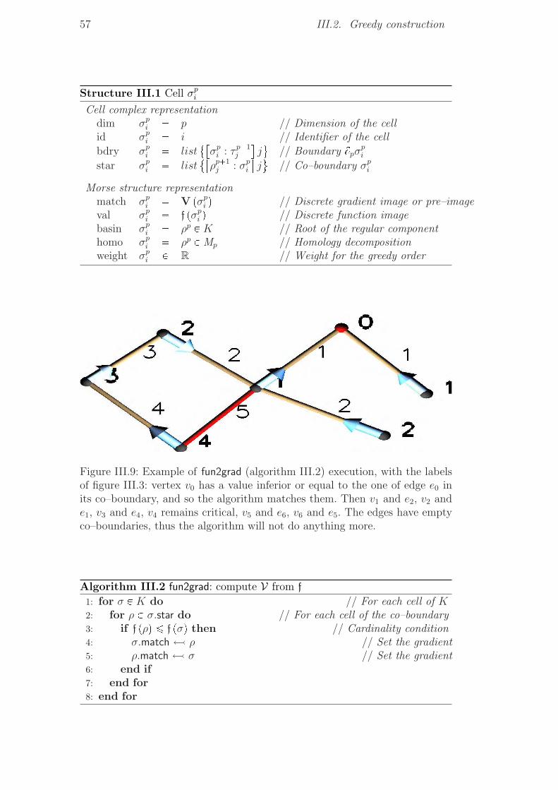
57 III.2. Greedy construction

Structure III.1 Cell σpi

Cell complex representationdim σp

i � p // Dimension of the cellid σp

i � i // Identifier of the cell

bdry σpi � list

�σp

i : τ p�1j

�j(

// Boundary Bpσpi

star σpi � list

�ρp�1

j : σpi

�j(

// Co–boundary σpi

Morse structure representationmatch σp

i � V pσpi q // Discrete gradient image or pre–image

val σpi � f pσp

i q // Discrete function imagebasin σp

i � ρp P K // Root of the regular componenthomo σp

i � ρp P Mp // Homology decompositionweight σp

i P R // Weight for the greedy order

Figure III.9: Example of fun2grad (algorithm III.2) execution, with the labelsof figure III.3: vertex v0 has a value inferior or equal to the one of edge e0 inits co–boundary, and so the algorithm matches them. Then v1 and e2, v2 ande1, v3 and e4, v4 remains critical, v5 and e6, v6 and e5. The edges have emptyco–boundaries, thus the algorithm will not do anything more.

Algorithm III.2 fun2grad: compute V from f

1: for σ P K do // For each cell of K2: for ρ P σ.star do // For each cell of the co–boundary3: if f pρq ¤ f pσq then // Cardinality condition4: σ.match ¾ ρ // Set the gradient5: ρ.match ¾ σ // Set the gradient6: end if7: end for8: end for


0 1 2 3 4

III.10(a): Original state.

0 1 2 3 4

III.10(b): Union of 0 and 1.

0 1 2 3 4

III.10(c): Union of 2 and 3.

0 1

2

3

4

III.10(d): Union of 2 and 4.

0

1

2

3

4

III.10(e): Union of 0 and 2.

Figure III.10: Example of union (algorithm III.3) executions.

Algorithm III.3 union(σ,τ) : union of the basins of σand τ

1: σ1 ¾ find(σ) // Get the basin of σ2: τ 1 ¾ find(τ) // Get the basin of τ3: if σ1.weight τ 1.weight then // σ1 is lower than τ 14: τ 1.basin ¾ σ1.basin // Assigns to the lower basin5: else // τ 1 is lower than σ16: σ1.basin ¾ τ 1.basin // Assigns to the lower basin7: end if


0

1

2

3

4

III.11(a): Find 1 returns 0.

0

1

2

3

4

III.11(b): Find 4 calls find 2.

0

1

2

3

4

III.11(c): Find 2 returns 0.

0

1

2 3

4

III.11(d): Find 4 updates 4.basin ¾ 0 and returns 0.

Figure III.11: Example of find (algorithm III.4) executions: each call updatesthe structure to optimize the next call.

Algorithm III.4 find(σ) : find the basin (root) of σ

1: if σ.basin � σ then // σis not the root of its basin2: σ.basin ¾ find(σ.basin) // Recursion3: end if4: return σ


construction and the Morse complex representation, since both are partitions

of the original cell complex constructed by cancellations, i.e. union of classes

in that partition. The Union & Find [Tarjan, 1975] data structure is an efficient

representation for these operations on such a partition. It is described in

algorithms III.3 (figure III.10) and III.4 (figure III.11).

(b) Greedy algorithm

The greedy construction of discrete Morse function starts with an empty

discrete gradient V (with all the cells critical) and adds pair per pair V ,

performing local cancellations of incident cells. A pair pτ σq is added if

neither τ nor σ already belong to a pair (discrete vector field condition)

and if this pair does not create any cycle inside V (gradient condition). The

second test (algorithm III.6) is the only complex part of the whole algorithm

(algorithm III.5). The implementation of the greedy construction is similar to

the spanning tree extraction (figure III.13): the links of the graphs are tested

sequentially, and if a link joins two distinct components, it is added to the

spanning tree. More precisely, the two nodes of a link belong to the same

component if the find algorithm returns the same root for both. In that case,

the link would create a cycle. Otherwise, the two components are joined by

the addition of the link, which is performed by a union operation.

Actually any discrete gradient V can be constructed with this algorithm,

by defining the weight of a cancellation such that only the pairs of V appear

in the priority queue.

III.12(a): The whole priorityqueue: cancelling apair invalidates otherelements of the queue.

III.12(b): The priority queue di-vided by half will havestored less pairs at theend of the algorithm.

Figure III.12: The priority queue of the greedy algorithm can be optimized.

Greedy algorithm. Since the greedy construction can generate any discrete

gradient, it depends heavily on its unique parameter: the cancellation weight

function, which induces the order for considering local cancellations. The


III.13(a): Union of v4 and v5 by e5.

III.13(b): Union of v3 and v4 by e4.

III.13(c): Union of v1 and v3 by e2.

III.13(d): Union of v3 and v5 by e6.

III.13(e): Union of v0 and v1 by e0.

III.13(f): Union of v0 and v2 by e1.

III.13(g): find(v0) = find(v2), thus e3 creates acycle and is not added.

Figure III.13: The spanning tree algorithm on the example of figure III.3.


III.14(a): Labeling of the torus. III.14(b): First 3 cancellations: v0 and e1,v4 and e0, v3 and e10.

III.14(c): 4 cancellations: e5 and f1, e8

and f2, e12 and f4, e14 and f5.III.14(d): 4 cancellations: v1 and e3, v2

and e17, v7 and e10, v8 and e13.Cancellation v2 and e6 wouldcreate a cycle.

III.14(e): 4 cancellations: e2 and f0, e9

and f3, e15 and f8, e16 and f7.III.14(f): The remaining cancellations

would create cycles, and v6, e6,e7 and f6 remain critical.

Figure III.14: The greedy algorithm on a torus model.


construction simply orders all the local cancellations with finite weight and

tests each of them sequentially (algorithm III.5 and figure III.14). Since the

cancellation pτ, σq prohibits any cancellation involving τ or σ, the algorithm

can be improved by considering in a first stage only the cancellations of weight

lower than a given threshold, then considering the valid cancellations of weight

below a second threshold and so forth. This improvement reduces the cost of

sorting the cancellations since the priority queue does not need to sort pairs

invalidated in previous stages (figure III.12).

Algorithm III.5 greedy(cancellation weight) : greedy construction of V1: priority queue tR�K �Ku ¾ H // Initialize the priority queue2: for σ P K do // For each cell of K3: σ.basin ¾ σ // Reset the Union & Find data structure4: σ.match ¾ 0 // Reset V5: for τ P σ.bdry do // For each cell of the boundary of σ6: w ¾ cancellation weight pK, pτ, σqq // Weight of the local

cancellation7: if w � 8 then // Allow selection of matchings8: priority queue.push ppw, τ, σqq // Sort the local cancellations9: end if

10: end for11: end for12:13: while pw, τ, σq ¾ priority queue.top do // Traverses the priority queue14: if σ.match � 0 and τ .match � 0 and not create cycle ppτ, σqq then //

the cancellation is valid15: σ.match ¾ τ // Set the gradient16: τ .match ¾ σ // Set the gradient17: for τ 1 P σ.bdry do // For each cell of the boundary of σ18: unionpτ 1, τq // updates the union & find data structure19: end for20: for σ1 P τ .star do // For each cell of the co–boundary of τ21: if σ1.match.dim � τ .dim then // σ1 belongs to the layer22: unionpσ1.match, τq // updates the union & find data structure23: end if24: end for25: end if26: end while

Acyclicity test. To test if the cancellation pτ σq would create a closed

hyperpath, the algorithm checks if the basin that would contain τ after the

cancellation already contains a node incident to σ (figure III.15). If the layer

contains only regular links, the test is the same as the spanning tree algorithm.


Algorithm III.6 create cycle(pτ σq) : test if pτ σq creates a cycle in V1: set tKu ¾ H // Get the basin of σ after the cancellation2: for σ1 P τ .star do // For each cell of the co–boundary of τ3: τ 1 ¾ σ1.match // Source of σ14: if τ 1.dim � τ .dim then // τ 1 belongs to the layer5: set.insert pfindpτ 1qq // Insert the basin of τ 16: end if7: end for8:9: for τ 1 P σ.bdry do // For each cell of the boundary of σ

10: if τ 1 � τ and τ 1.match.dim � σ.dim then // τ 1 belongs to the layer11: ρ ¾ find(τ 1) // Get the basin of τ 112: if ρ P set then // The basin ρ contains a node incident to τ13: return true // The cancellation would create a loop14: end if15: end if16: end for17: return false // The cancellation is valid

01

2

3

4

56

7

8

9

10

11

12

13

14

2021

2223

24

25

26

27

28

30

40

41

4243

44

4647

48

49

45

5152

5354

50

60

61

62

63

64

65

6667

68

69

7172

73

74

70

100

Figure III.15: The cancellation of node σ � 0 and the hyperlink τ �t0, 24, 27, 73u would create a cycle since 73 and the nodes 64 or 70 are inthe same component. Without the node 73 in the hyperlink, the cancellationwould have been valid.

Gradient integration. The last step of the algorithm is to generate a

discrete Morse function from the gradient. As we already mentioned, there

are infinitely many discrete Morse functions corresponding to a gradient, as

we can for example scale any connected component. However, any of these

discrete Morse functions must be increasing along the gradient. In that sense,


0

1

2

3

4

5

6 7

8

9

10

11

12

13

14

1516

1718

19

20

21

23

24

25

26

22

28

29

30

31

27

32

III.16(a): Labels: there are 4 roots: 7 and 32,22 and 27.

99

98

97

96

100

III.16(b): Starting from node 32: the stack,until line III.7, contains onebranch.

99

98

97

96

96

100

III.16(c): Then pops the stack, confirmsvalue 96 and continues.

9998

98

97

97

97

96

96

96

97

96

96

96

96

96

100

III.16(d): Completes the component of node32.

97

96

95

95->98 100

99

98

9998

98

97

97

97

96

96

96

97

96

96

96

96

96

100

III.16(e): Starts from node 7: the branchreaches nodes 6 which is alreadyassigned, and increases the storedvalue of m.

100

99

99

98

98

95

98 104

99->103

103

102

101

102

102

101

101100

9998

98

97

97

97

96

96

96

97

96

96

96

96

96

100

III.16(f): Completes the component of node7: the value needs to be increasedagain from node 10 to node 8, butnot from node 27 to node 7.

Figure III.16: Example of grad2fun execution (algorithm III.7).


the construction of algorithm III.7 is the simplest one, assigning to each cell

its depth in its layer hyperforest (figure III.16). The algorithm assigns first

a Morse value to the nodes of each regular component and assigns the same

value to the destination link. If it encounters a hyperlink entering to a regular

component, it follows that link to assign first the lower regular component.

Therefore, the assignment must be done from the leaves to the roots in order

to maintain a node with a higher value than its sons.

Algorithm III.7 grad2fun : compute f from V1: for p P r1 . . . dim Ks do // For each layer hyperforest2: m ¾ 2 � card Kp // Value big enough to separate layers3: for σ P roots ofLppp�1q, ( do // Get the minimal root4: stack tDualpYCritp � Primp�1Yt0uu ¾ tpσ, 0qu // Traversal stack5: while stack � H do // Regular component traversal6: σ ¾ stack.top // Get the first cell of the path7: while D τ σ, unmarked pτq do // Still not the leaf8: σ ¾ τ.match // Completes the gradient step9: stack.push ppσ, τqq // Stores the gradient step

10: mark pσq ; mark pτq // Marks step as visited11: m ¾ m� 1 // Down one depth level in the tree12: end while13: // Reached a leaf14: pσ, τq ¾ stack.top // Get the last step of the path15: M � max val

τ 1 σ, marked pτ 1q , τ 1 P Lppp�1q, τ 1 non regular

(// Maximum of assigned non–regular links

16: m ¾ max pm,M � 2q // Maintain increasing f

17: if τ � 0 then // Non–critical cell18: σ.val ¾ m ; τ.val ¾ m // Assign matched cells19: end if20: m ¾ m� 1 // Up one depth level in the tree21: end while22: end for23: end for24:25: for ρ P K do // For the unassigned critical cells26: if ρ.val � unassigned then // ρ unassigned27: ρ.val � max val tDualdim ρYCritdim ρu � 1 // Assigns a critical value28: end if29: end for

(c) Heuristic for optimal Morse functions

In [Lewiner, 2002], our goal was to define optimal discrete Morse func-

tions, i.e. Morse functions having the minimal possible number of criti-

cal cells. This problem has been proved NP–hard [Lewiner et al., 2003b,


Joswig & Pfetsch, 2005]. An exponential algorithm can be simply implemented

testing all possible matchings, or in a more elegant way using integer pro-

gramming [Joswig & Pfetsch, 2005]. However, the greedy algorithm above can

be used to compute discrete Morse functions with a very small number of

critical cells (algorithm III.8). On the models of [Hachimori Models], this

algorithm always reached the optimum in less than quadratic time. More-

over, it has been proved to reach the optimum for surfaces in almost linear

time [Lewiner et al., 2003a].

Since the regular part of the hypergraphs is easier to process, the

algorithm calls first the greedy procedure for each layer separately, considering

only the regular links (figure III.17). Then it prunes the layer hypergraph.

If there is no more leaves in an non–empty layer, there is a cycle of valid

cancellations. This cycle is broken arbitrarily (here is the heuristic), using the

matching of higher cancellation weight. To do so, we call “once” the greedy

algorithm, where once command on line III.8 of the algorithm means that

greedy performs only one valid matching and returns.

Algorithm III.8 optimal(cancellation weight) : Construction of an optimal V1: for d P t1, . . . , dim Ku do // Process layers separately2: define weight pK, pτ, σqq ¾ // Discards non–regular links$'&'%8 if σ.dim � d

8 if σ is not a regular link of Lpd�1qdcancellation weight pK, pτ, σqq otherwise

3: greedy(weight) // Construction of the regular components of Lpd�1qd4: end for5:6: repeat // Pruning and greedy step7: define weight

�τ d�1, σd

�¾ // Pruning$'&'%cancellation weight pK, pτ, σqq if τ is a leaf of Lpd�1qd

cancellation weight pK, pτ, σqq if σ is a leaf of Ldpd�1q8 otherwise

8: greedy(weight) // Primal and dual pruning9: once greedy(cancellation weight) // Unlock cancellation cycles

10: until no more valid local cancellation

(d) Complexity

The acyclicity test of algorithm III.6 performs in time O ps � log sq, where

s is the average size of the boundary and co–boundary of a cell. We will suppose

that for a complex K, this size is in average bounded by a small constant. This

implies that algorithm III.6 has in average a constant complexity.


III.17(a): First call to greedy with d = 1 (layer L01). III.17(b): Layer L01 on thetorus.

1

3

5

7

8

9

18

10

11

13

16

26

19

27

28

30

33

3435

38

39

41

42

63

44

46

47

49

50

51

53

56

58

III.17(c): Second call to greedy with d = 2 (layer L12).

III.17(d): Third call to greedy with d = 3 (layer L23). III.17(e): Layer L23 on thetorus.

III.17(f): Last call to greedy: pruning layer L12. III.17(g): Layer L12 on thetorus.

Figure III.17: Example of optimal execution (algorithm III.8) on a solid torus.


The Union & Find structure of algorithms III.3 and III.4 has complexity

O pα pnqq, where α pnq is the inverse Ackermann function [Tarjan, 1975]. In

fact, this function has a value less than 5 for any conceivable input size

(table III.18). Since then, the complexity of the Union & Find structure is

often called almost constant.

The greedy construction of algorithm III.5 first creates the priority queue,

and then calls for each candidate matching the acyclicity test of algorithm III.6,

and eventually O psq times the union function. Since we considered that s is in

average constant, the second part of the algorithm is almost linear. If the can-

cellation weight does not matter, for example if cancellation weight pK, pτ, σqqis constant, the priority queue is created in a time linear to the number of

matchings O ps �#Kq � O p#Kq. If the cancellation weight is significant, the

priority queue has complexity O p#K � log #Kq.n P α pnqt1, 2, 3u 1t4, 5, 6, 7u 2t8, . . . , 61u 3#

62, . . . , 222222

2

� 3

+4

Table III.18: Inverse Ackermann function values.

Finally, the complexity of the optimal construction is a priori the same as

the greedy construction, i.e. either O p#K � log #Kq if the cancellation weight

must be respected, or O p#K � α p#Kqq on the contrary. However, the second

loop of the algorithm can require a time quadratic in the number of remaining

cancellations. Observe that there is at most h remaining cancellations, where

h is the number of non–regular hyperlinks. The final complexity is therefore

usually linear, and quadratic in the worst case [Lewiner, 2002].

(e) Application to volumetric compression

Among the different strategies to compress polyhedral meshes, most

of the state–of–the–art approaches [Rossignac, 1999, Lopes et al., 2002,

Lewiner et al., 2004, Touma & Gotsman, 1998, Alliez & Desbrun, 2001,

Kalberer et al., 2005] for surfaces encode the connectivity of the mesh by

a traversal equivalent to a dual layer of a discrete gradient V . The roots of the

layer are the most expensive elements to encode. In order to minimize those

elements, the algorithm tends to optimize V , since each critical cell is a root.

In the case of surfaces, we proved in [Lewiner et al., 2003a] that any spanning

forest reaches the optimum.


Figure III.19: Because of the critical edge (in red), the green triangle must bea dual cell, isolated inside the dual hyperforest. This triangle will be expensiveto encode.

However, for 3–manifolds, the problem is NP–hard and re-

quires some heuristics to be quickly resolved. The strategy of algo-

rithm III.8 is similar for that special case to the one used by Grow &

Fold [Szymczak & Rossignac, 2000], as described in [Lewiner et al., 2004].

This heuristic actually generalizes to higher dimensions and to non–manifold,

non–simplicial and non–pure cell complexes, which can be useful for further

compression algorithms.

III.3 Flow basins and hypergraph components

The representation of a discrete gradient as hyperforests simplified the

algorithmic construction of discrete Morse functions. Actually, this represen-

tation turned out to be more meaningful than just an efficient data structure.

This section shows the close relation between the regular components of a

layer Lppp�1q pVq (section III.1(c) Hyperforest) and the unstable basin of the

flow W uV pσpq (section II.7(b) Invariant chains). Actually, the Union & Find data

structure represents almost directly those unstable basins W uV . This will en-

hance the representation of both the discrete Morse–Smale decomposition and

the Morse homology computation. In order to compute the unstable basins, we

will consider only dual layers. The stable basins can be obtained in a similar

way using the primal layers instead, although those were not explicitly defined

in Forman’s original works.

(a) Flow image of a critical or dual cell

Consider a node n of the dual layer Lppp�1q pVq. This node represents a

cell σp that is either dual or critical. The sons of n are the nodes n1 of Lppp�1qthat are sources of links incident to n: n ù n1 if Dl : n ¡ l and pl, n1q P V . We

will say that n is the father of the n1. The iterated son of a node n is either

the son of n or the son of an iterated son of n. We will prove now the following

proposition:

71 III.3. Flow basins and hypergraph components

Proposition 2 The flow image Φ pσpq of σp is composed of the sons of n plus

n itself if σp is critical.

Proof : The flow of σp is defined as (section II.7(b) Invariant chains):

Φ pσpq � σp �V pBp pσpqq � Bp�1 pV pσpqq (1)

Independently if σp is dual or critical, V pσpq � 0, which simplifies the right

term of the equation. Now the boundary Bp pσpq of σp is composed of cells τ p�1

that belongs either to Lppp�1q or to Lpp�1qpp�2q. The latter case implies that τ p�1

is either dual or critical, which means its image through V is zero. Therefore,

we get:

Φ pnq � n�V

�� ¸lPPrimpp�1q,l n

rn : ls � l� (2)

III.20(a): 1 iteration. III.20(b): 3 iterations. III.20(c): 4 iterations.

Figure III.20: Iterated flow image of a critical cell on a dual layer: the criticalcell is included in its image.

Image of a critical node. From the definition of son, each son of n is

the image by V of a term of the sum of equation (2). On one hand, if n is

critical, it is not the image of any link, and will therefore be part of its image

through the flow (figure III.20). On the other hand, each term of the sum of

equation (2) is mapped by V to a son of n. Therefore, we get:

Φ pnq � n� ¸n1øn

rn : ls � rn1 : ls � n1 (3)

The coefficient of each son n1 actually corresponds to the multiplicity of the

gradient path µ p� n l n1 �q.

Image of a dual node. If n is not critical, it is the image of a link ln which

appears in the sum of equation (2). The other terms of the sum behave like

the critical case:

Φ pnq � n� rn : lns �V plnq � ¸n1øn

µ p� n l n1 �q � n1 (4)

From the orientation of the gradient, the terms with n cancels (figure III.21),

and we get:


III.21(a): 0 iteration. III.21(b): 1 iteration.

III.21(c): 2 iterations. III.21(d): 3 iterations.

Figure III.21: Iterated flow image of a dual cell: the image vanishes after anumer of iterations equal to the depth of the connected component.

Φ pnq � ¸n1øn

µ p� n l n1 �q � n1 (5)

¥We can deduce from this calculus the following result of [Forman, 1995]:

Corollary 3 The iterated flow of a dual node vanishes:

σ P Dual pVq ñ Φ8 pσq � 0 .

Proof : Iterating equation (5), we get:

Φk pσpq � ¸n0øσp

¸n1øn0

. . .¸

nkønk�1

µ p� σp n0 n1 . . . nk �q � nk (6)

Since there is no closed hyperpath in a hyperforest, the length of the hyper-

path starting from σp is bounded by a particular k. With the notation of

equation (6), there is no nk�1 son of nk, and there is no term in the sum of

Φk�1 pσpq. ¥

(b) Discrete stable and unstable basins

From the above result, we can already compute the unstable basins

directly from the layer representation.


Theorem 4 The unstable basin Φ8 pσpq P CΦp of a critical cell σp contains the

regular component of σp in Lppp�1q and is contained in the connected component

of σp in Lppp�1q.Proof : The theorem is a simple consequence of propositions 1 and 2. From

proposition 2, the flow image of a critical cell contains the critical cells.

Therefore the elements of the image accumulate, and we get that:

Φkpσpq � σp � ¸n0øσp

µ p� σp . . . n0 �q ��

n0�¸n1øn0

µ p� n0 n1 �q ��

n1 � . . .¸

nkønk�1

µ p� nk�1 nk �q � nk

� (7)

From the last part of proposition 1, the fathers of the nodes of the regular

component of σp belongs to the regular component of σp. There is thus no

cancellation inside the sum of terms belonging to the regular component of σp.

From equation (7), the last part of the theorem is obvious. ¥

Figure III.22: Integral paths from both critical nodes 7 (in green) and 32 (inblue) merge on root 22 (red).

Integral path merging. Observe that a strong difference between smooth

and discrete Morse theories is that a cell can belong to several stable basins

at the same time (figure III.22). This is due to the definition of integral path

that allow two paths to merge. In the smooth setting, the uniqueness of the

solution of ordinary differential equations ensures that two integral curves

can become arbitrarily close, but not merge. In the discrete setting, integral

path can obviously not become arbitrarily close. In particular, this induces


that a node can be the iterated son of a critical cell and not belongs to its

unstable basin. This occurs for example when a node is at the junction of two

integral path, and when the multiplicity of the first one is the opposite of the

multiplicity of the second one. However, this will be solved gracefully the case

of homology cycles that share cells.

Stable basins. The considerations of this chapter apply directly for the sta-

ble basins, when considering primal layers instead of dual ones. For manifolds,

this can be also been proved by considering the dual manifold with the dis-

crete Morse function �f (i.e. reverting the pairs of V). The dual layers become

primal layers, and the unstable basins become stable basins.

Theorem 5 The stable basin of a critical cell σp contains the regular com-

ponent of σp in Lppp�1q and is contained in the connected component of σp in

Lppp�1q.

(c) Flow image of a primal cell

0

4

7

8

9

10

11

12

14

17

III.23(a): Labeling. III.23(b): 0 iteration.

III.23(c): 1 iteration. III.23(d): 2 iterations.

Figure III.23: Flow iteration on layer L12 of figure III.14: while the flow of 4vanishes, the flow of 11 reaches critical edge 17.

The dual layer has simplified the expression of the flow of a dual cell,

since the image of a dual node is the sum its sons in the dual layer Lppp�1q.We reach a similar result for the primal cells, and we will therefore use the


primal layer Lpp�1qp. The primal and dual layers differ in one point, noted in

proposition 1: the orientation of the dual layer goes towards the roots, while

the orientation foes outwards in a primal layer (figure III.23). This means in

particular that the son of a primal cell can be a critical cell, and therefore its

image under the iterated flow cannot vanish.

Since the image of a cell by V is always a dual cell (section III.1(a) Cell

classification), we can write equation (1) as follow:

Φ�τ p�1

� � τ p�1 � Bp

�V�τ p�1

��Dualp�1 (8)

From corollary 3, the terms of Dualp�1 will vanish when iterating the flow.

Observe that V pτ p�1q is the link ln having the node n representing τ p�1 as

source. The boundary of ln is then composed of dual cells, n itself and the sons

of n in Lpp�1qp:

Φ pnq � n� rln : ns � rln : ns � n� ¸n1øn

µ p� n ln n1 �q � n1 (9)

The first two terms cancels. If n has no iterated son that is critical, its iterated

flow will vanish:

Theorem 6 The iterated flow of a primal pp � 1q–cell n vanishes if it has a

no critical iterated son. More generally, the iterated flow of n is the sum of the

iterated flow of the critical iterated sons of n:

Φ8 pnq � ¸ρPCritp�1

¸� nùn0...nkùρ �

µ p� n ù n0 . . . nk ù ρ �q �Φ8 pρq (10)

This result allows an enhanced computation of the decomposition of a cycle on

the Morse–Witten homology base. In particular, since Lppp�1q is a hyperforest,

the nodes leading to a critical node are easily identified. The only problem could

come from two hyperpath leading to the same critical node, and cancelling it.

This requires a path merge that only occur on non–regular link. That is why

we will first concentrate on the regular parts of the layers, in particular for the

proofs of the last chapter.

IVHomology computation

Homology is a simple combinatorial invariant of geometrical objects.

Particularly for high–dimensional cell complexes, it offers a direct classifica-

tion that helps distinguishing models, checking their validity and even cor-

recting them. However, the cost of homology computation is still a prob-

lem for big amount of data. The classical method for computing homology

relies on the Smith normal form [Dumas et al., 2003]. This method is es-

sentially a Gaussian pivoting, which becomes very costly when the size of

the complex increases. In the specific case of sub–triangulations of S3, the

Betti numbers on Z2 can be computed using Mayer–Vietoris sequences in

time O p#K � α p#Kqq [Delfinado & Edelsbrunner, 1993, Dey & Guha, 1998].

A basis of generator of the homology can be obtained for this very restrictive

case with the same complexity.

Homology computation was at first an attempt to define properly the crit-

ical cells of the geometric Morse complex of the next chapter. However, the al-

gorithms introduced here outperform most of the known algorithm. In particu-

lar, it computes with the same complexity as [Delfinado & Edelsbrunner, 1993,

Dey & Guha, 1998] the Betti numbers, but without restriction on the cell com-

plex or on the field of coefficients. They further compute the complete homol-

ogy groups on any field, provide an explicitly basis for these groups on the

complex and compute the decomposition of any cycle on that basis. The first

part of this chapter introduces the tools used by the second part, which con-

tains the detailed description of these algorithms.

IV.1 Algebraic and combinatorial tools

Homology can be completely computed from the Smith normal forms.

However, even with the optimizations of this normalization (for example

using [Dumas et al., 2003]), it is still an expensive operation. In particular

when computing the homology of real geometrical models, that have usually

millions of cells, this computation can be prohibitive, even if the topology of

those models is trivial! We propose here to reduce drastically the complexity of

Chapter IV. Homology computation 78

this calculus, by computing the homology on the Morse complex instead of the

whole complex. We know from section II.8(b) Witten–Morse homology that both

are equivalent, but the Morse complex is usually much smaller. Particularly

for usual geometrical models with millions of cells, if the topology is trivial

then the Morse complex will have only a few cells.

(a) Smith normal form

Consider a cell complex K and a ring K for the coefficients of the chains.

To clarify the presentation, we can think that K � Z2 or K � Z, but the whole

chapter is valid on any computable ring. Since the chain modules are freely

generated by the cells of K, the boundary operator Bp : Cp Ñ Cp�1 can be

represented by a rectangular matrix Bp of size #p�1 � #p with coefficient in

K. For example the boundary of an edge σ is the difference of its end vertices

τ1 and τ2. This means that in the matrix of B1, the line indexed by σ will have

exactly two non–null entries: a �1 for τ2 and a �1 for τ1.

Recall that the homology groups of K are Hp � ker Bp{ Im Bp�1. We will

try to find a basis for Cp on which both ker Bp and Im Bp�1 will be diagonal.

The main tool to do so is the Smith normal form, which is a conjugation of

matrices obtained by the Gauß operations on lines and columns in order to let

the considered matrix diagonal. The coefficients of the diagonal will be either

0 or other elements of K totally ordered by division. More precisely, the Smith

normal form of a matrix Mm�n is given by the two invertible matrices Pm�m

and Qn�n such that:

Pm�m �Mm�n �Qn�n �

��k1 0 ... 0 0 ... 0 ... 00 k2 ... 0 0 ... 0 ... 0...

......

......

0 0 ... kr 0 ... 0 ... 00 0 ... 0 0 ... 0 ... 0...

......

......

......

0 0 ... 0 0 ... 0 ... 0

�� with 0 � k1 | k2 | . . . | kr

With this Smith normal form, we will build a base c1 � � � c#p

(of Cp

such that ker Bp will be generated from tc1 � � � cru and Im Bp�1 will be generated

from cr�1 � � � c#p

(. Let P#p�1�#p�1 and Q#p�#p be the matrices of the Smith

normal form of Bp:

P �Bp �Q ��

Kr�r 0r�p#p�rq0p#p�1�rq�r 0p#p�1�rq�p#p�rq

�.

Observe that K is diagonal. Since Bp � Bp�1 � 0, we have Bp � Bp�1 � 0.

79 IV.1. Algebraic and combinatorial tools

Therefore P �Bp �Bp�1 � 0:�Kr�r 0

0 0

��Q�1 �Bp�1 � 0 and thus Q�1 �Bp�1 �

�0r�#p�1

Bp�1

�We can now apply the Smith normal form on Bp�1, which is of size p#p � rq�#p�1, using matrices Pp#p�rq�p#p�rq and Q#p�1�#p�1 :

P � Bp�1 � Q ��

Kr�r 0r�p#p�1�rq0p#p�r�rq�r 0p#p�r�rq�p#p�1�rq

�.

Observe that K is also diagonal. Let R#p�#p ��1r�r 0

0 P

�. We can then write:

R �Q�1 �Bp�1 � Q �� 0r�r 0r�p#p�1�rq

Kr�r 0r�p#p�1�rq0p#p�r�rq�r 0p#p�r�rq�p#p�1�rq

�� .

b1

b2

b3

br−1

brbr+1

b#p−1

c1

c2

c3

cr−1

crcr+1

cr+r−1

cr+rcr+r+1

c#p

d1

dr−1

drdr+1

d#p+1

d2

d3

{0} {0}

∂p+1

∂p+1

∂p

∂p

Figure IV.1: Two Smith normal forms are used to decompose the boundaryoperator.

Now we can build the bases tdiu, tciu and tbiu for Cp�1, Cp and

Cp�1 respectively (figure IV.1). Let tτiu � tτ p�1 P Ku, tσiu � tσp P Kuand tρiu � tρp�1 P Ku be the canonical basis of Cp�1, Cp and Cp�1. Then

di � P�1 � rτjsj, ci � QR�1 � rσjsj and bi � Q � rρjsj.


We can then express Bp and Bp�1 on these bases:

Bp pciq � pP�1Pq �Bp � pQR�1σiq � P�1 ��Kr�r 0

0 0

��1r�r 0

0 P�1

�� σi

�$&%kidi i ¤ r

0 i ¡ r

Bp�1 pbiq � pQR�1 �RQ�1q �Bp�1 � Q τi � QR�1 ��0 0

K 0

0 0

�� τi

�$&%kicr�i i ¤ r

0 i ¡ r.

The homology group Hp � ker Bp{ Im Bp�1 can then be written in terms of the

coefficient of K and K: Hp � Kk1cr�1,Kk2

cr�2, . . .Kkrcr�r ¡. Oberver that

since Bp pciq � 0 for i ¡ r, the basis chains ci are cycles for i ¡ r.

(b) Boundary operator on the Morse complex

Consider now a cell complex K, with a discrete gradient V defined on

it. V is not necessarily optimal, but the homology computation will be more

efficient if it has less critical cells. We would like to compute explicitly the

boundary operator Bp : Mp Ñ Mp�1 on the Morse complex, where Mp is the free

module generated by the critical p–cells of V . Recalling the diagram of section

II.8(b) Witten–Morse homology:

t0u C0B0oo

Φ8²²

C1B1oo

Φ8²²

C2B2oo

Φ8²²

� � �B3oo CnBnoo

Φ8²²

t0uBn�1oo

t0u CΦ0

B0oo

Id

OO

X²²

CΦ1

B1oo

Id

OO

X²²

CΦ2

B2oo

Id

OO

X²²

� � �B3oo CΦn

Bnoo

Id

OO

X²²

t0uBn�1oo

t0u M0B0oo

Φ8OO

M1B1oo

Φ8OO

M2B2oo

Φ8OO

� � �B3oo MnBnoo

Φ8OO

t0uBn�1oo

we can define B by Bp pσpq � Bp pΦ8 pσpqqXMp�1. Since the boundary operator

commutes with the flow (Bp �Φ � Φ � Bp), we will use the following formula for

the boundary operator on Mp: Bp pσpq � Φ8 pBp pσpqq XMp�1.

In terms of layers of V , the boundary of a critical p–cell is made of dual,

primal and critical pp � 1q–cells. From corollary 3, the iterated flow of a dual

cell vanishes. From equation (3) of section III.3(a) Flow image of a critical or

dual cell , the only critical cell in the iterated flow of a critical cell τ p�1 is τ p�1

itself. We can thus compute the boundary operator of a critical cell σp directly


Figure IV.2: The boundary operator can be read directly on the layer lookingat the connection between the critical cells as nodes (red nodes) and the criticalcells as links (red links).

on layer Lpp�1qp, using theorem 6 as:

Bp pσpq � ¸τp�1PBppσpqXCritp�1

�σp : τ p�1

�τ p�1 �

¸nPBppσpqXPrimp�1

¸ρPCritp�1

¸� nù...ùρ �

µ p� n ù . . . ù ρ �q � ρ(1)

Although equation (1) seems complex, it is easily implemented by algo-

rithm IV.1 (figure IV.3). Since our representation of V on structure III.1 maps

a cell to its root, it is easier to get the iterated father of a cell than its iterated

son. We will thus compute the boundary matrix Bp by the co–boundary Bp,

whose matrix is the transposed BTp of Bp. We need to modify the union proce-

dure (algorithm III.3) to store directly at the gradient creation the multiplicity

of the unique path of a cell to its root:

pσ.basinqµ �¸

� σø...øσ.basin �µ p� σ ø . . . ø σ.basin �q .


Algorithm IV.1 boundaryppq : boundary operator on the Morse complex ofV1: if card pCritpq � card pCritp�1q � 0 then // Trivial case2: return H3: end if4: Bp ¾ 0K // Initializes the matrix5: for τ P Critp�1 do // Critical pp� 1q–cells6: stack tDualp�1YCritp�1�Ku ¾ tpτ, 1Kqu // Hyperpath storage7: while stack � H do // Hyperpath traversals8: pτ 1, µq ¾ stack.top // Get the first cell of the path9: for σ P τ 1.star X pPrimpYCritpq do // For each primal or critical

cell of the co–boundary of τ 110: ρ ¾ σ.basin // Accesses the root11: µ1 ¾ µ � pσ.basinqµ � rσ : τ 1s // Path multiplicity12: if ρ P Critp then // Critical root13: Bprτ srρs ¾ µ1 �K Bprτ srρs // Adds to the matrix14: continue // End of hyperpath15: end if16: ρ1 ¾ ρ.match // Unique outgoing link of the hyperpath17: µ1 ¾ rρ : ρ1s � µ1 // Path multiplicity18: if ρ1 � τ 1 then // Valid path extension19: stack.push ppρ1, µ1qq // Stores the path extension before next σ20: end if21: end for22: end while23: end for24: return Bp // Result


IV.3(a): Original model.

0

1

2

4

+-

14

-

-

5

6

7

12

1316-

+

17

-

-

18

22

32-

-

2324

25

29

30+

-

31

33

-

+

34

-

+

+

+

+

+

+

+

-

-

+

-

+

+

-

-

-

+

+ +

++

+

-

+

-

+

+

-

-

-

-

IV.3(b): Labeling of layer L12 withthe critical faces.

+-

-

-

-

+

-

-

-

-

+

--

+

-

+

+

+

+

+

+

+

-

-

+

-

+

+

-

-

-

+

+ +

++

+

-

+

-

+

+

-

-

-

-

IV.3(c): Looks in the star of the criticallinks.

+-

-

-

-

+

-

-

-

-

+

--

+

-

+

+

+

+

+

+

+

-

-

+

-

+

+

-

-

-

+

+ +

++

+

-

+

-

+

+

-

-

-

-

IV.3(d): Takes the root of the active cell:there is a negative incidence onthe critical node.

+-

-

-

-

+

-

-

-

-

+

--

+

-

+

+

+

+

+

+

+

-

-

+

-

+

+

-

-

-

+

+ +

++

+

-

+

-

+

+

-

-

-

-

IV.3(e): If the active cell is not critical,iterates on its matched cell.

+-

-

-

-

+

-

-

-

-

+

--

+

-

+

+

+

+

+

+

+

-

-

+

-

+

+

-

-

-

+

+ +

++

+

-

+

-

+

+

-

-

-

-

IV.3(f): Takes the root again.

+-

-

-

-

+

-

-

-

-

+

--

+

-

+

+

+

+

+

+

+

-

-

+

-

+

+

-

-

-

+

+ +

++

+

-

+

-

+

+

-

-

-

-

IV.3(g): Iterate: the top critical linkhas an empty boundary on theMorse complex.

+-

-

-

-

+

-

-

-

-

+

--

+

-

+

+

+

+

+

+

+

-

-

+

-

+

+

-

-

-

+

+ +

++

+

-

+

-

+

+

-

-

-

-

IV.3(h): The matched hyperlink cancelsthe critical node with a positiveincidence.

Figure IV.3: Example of boundary (algorithm IV.1) execution: the executionlooks synchronous but a stack allows computing each part separately.


IV.2 Complete homology calculus

The algorithms we will introduce now are direct applications of section

II.8 Morse complexes, using the optimal construction of section III.2(c) Heuristic

for optimal Morse functions to reduce the computational costs. They first

compute an optimal discrete gradient, and then compute the homology on the

Morse complex generated. Since this Morse complex is generally composed of

only a few cells, any algorithm will be almost instantaneous. These algorithms

actually work with any discrete gradient, but they will be more efficient on

optimal ones. For example, to use the Smith normal form method, all we need

is the matrix representation of the boundary operator we just computed. The

iterated flow then links back the homology of the Morse complex onto the

original complex. It can be efficiently computed on the hypergraph structure

we introduced in the last chapter, using the results of equation (3), corollary 3

and theorem 6 of section III.3 Flow basins and hypergraph components.

(a) Betti numbers and torsion

If we only need the Betti numbers over Z2 or Q or R, we do not

need to compute the whole Smith normal form, since there is no torsion.

In that case, it is sufficient to compute the ranks of Bp and Bp�1 to get

βp � rankBp � rankBp�1. In the general case, the complete homology group

is composed of the free part of degree βp plus the torsion. It can be computed

by algorithm IV.2. Observe that although the algorithm calls the optimal

procedure, it works even if the discrete gradient is not optimal.

Algorithm IV.2 homologypKq : compute the homology groups

1: optimalp0q // Computes an optimal discrete gradient2: B�1 ¾ 0K // For joint reduction3: for p P t0, . . . , dim Ku do // Get the matrices of the boundary operator4: Bp ¾ boundary ppq // Original matrix

5:�Bp,Pp,Qp

¾ smith pBp,Bp�1q // Normal form on the basis of Bp�1

6: rp � rank Bp // Rank of the boundary operator7: for i P trp�1, . . . , rp�1 � rpu do // Homology group8: cp�1,i � Qp�1P

�1p � rσjsj // Compute the basis

9: kp�1,i � Bprisris // Compute the basis10: end for11: βp�1 � card tkp�1,i � 1K, i P trp�1, . . . , rp�1 � rpuu // Betti number12: end for13: return

!Hp � Kkp,1cp,rp�1, . . .Kkp,rp�1

cp,rp�rp�1 ¡, p P t0, . . . , dim Ku)The complexity of algorithm IV.2 is the one of the optimal procedure,

85 IV.2. Complete homology calculus

O p#K � α p#Kqq (section III.2(d) Complexity) plus the complexity of the Smith

normal form on the critical cells, which is in the worst case O�m3

p

�. Observe

that this algorithm computes the Betti numbers, the torsion and a set of

generators for the homology on the Morse complex.

(b) Generators

IV.4(a): Critical cells.

IV.4(b): Pruned iterated flow of the two critical faces.

IV.4(c): Pruned iterated flow of the six critical edges.

Figure IV.4: Almost pruned iterated flow images of the critical faces and edgeson a double torus.

The elements cp�1,i are the generators of the homology on the Morse

complex: in the simple cases, cp�1,i is simply one critical cell. In order to

obtain a set of generators on the original complex, we need to map them

back onto the original complex K. We know from section II.8(b) Witten–Morse

homology that this mapping involves the iterated flow Φ8. The invariant chain

Φ8 pcp�1,iq always contains a generator of the homology groups on the original

complex (figure IV.4), but it generally contains other cells and is therefore not


Figure IV.5: Pruning a chain to get a cycle.

-+

-

+

-

+

+

-

-+

-

+

+-

-

+

+-

+

-

+

-

-

+

-

+

-

+

+

-

-+

-

+ +-

-

+

-

++

-

+

-

IV.6(a): On layer L21 of figure IV.3(a), theinvariant chains begins at the criti-cal nodes.

-+

-

+

-

+

+

-

-+

-

+

+-

-

+

+-

+

-

+

-

-

+

-

+

-

+

+

-

-+

-

+ +-

-

+

-

++

-

+

-

IV.6(b): Adding the sons (with their sign) tothe invariant chain.

-+

-

+

-

+

+

-

-+

-

+

+-

-

+

+-

+

-

+

-

-

+

-

+

-

+

+

-

-+

-

+ +-

-

+

-

++

-

+

-

-+

-

+

-

+

+

-

-+

-

+

+-

-

+

+-

+

-

+

-

-

+

-

+

-

+

+

-

-+

-

+ +-

-

+

-

++

-

+

-

-+

-

+

-

+

+

-

-+

-

+

+-

-

+

+-

+

-

+

-

-

+

-

+

-

+

+

-

-+

-

+ +-

-

+

-

++

-

+

-

-+

-

+

-

+

+

-

-+

-

+

+-

-

+

+-

+

-

+

-

-

+

-

+

-

+

+

-

-+

-

+ +-

-

+

-

++

-

+

-

IV.6(f): The resulting invariant chain is al-ready pruned on that simple exam-ple.

Figure IV.6: Example of generators (algorithm IV.3) execution.


a cycle: Bp pΦ8 pcp�1,iqq � 0. In order to get a set of generators on the original

complex, the simplest method is to prune the invariant chains Φ8 pcp�1,iq until

they become cycle (figure IV.5). At each step of the pruning, a cell is removed

from the chain Φ8 pcp�1,iq if it is adjacent to only one other cell of Φ8 pcp�1,iq.Algorithm IV.3 and figure IV.6 illustrate this procedure.

Algorithm IV.3 generators(cp,i) : computes a set of generators on the originalcell complex

1: // Compute the iterated flow2: stack tDualpYCritp�Ku ¾ H // Stores flow front3: for pσ, µq P cp,i do // For each cell of the chain4: stack.push ppσ, µqq // Initial chain5: end for6: b ¾ 0 // Iterated flow of cp,i

7: while stack � H do // Iterate the flow8: pσ, µq ¾ stack.top // Get a cell of the chain9: b ¾ b� µ � σ // Adds the cell to the invariant chain

10: for τ P σ.bdry X Primp do // Links of σ in Lppp�1q11: σ1 ¾ τ.match // Unique outgoing node of the hyperlink12: µ ¾ rτ : σs � rτ : σ1s � µ // Path multiplicity13: stack.push ppσ1, µqq // Stores for path extension14: end for15: end while16:17: // Prune the invariant chain18: boolean invariant ¾ false // Invariance marker19: repeat20: boolean invariant ¾ true // Not changed yet21: for τ P Bb do // cells that prevent b from being a cycle22: b ¾ bzτ.star // Prune the generator of the spurious boundary23: invariant ¾ false // Invariant when Bb � 024: end for25: until invariant // Pruned

(c) Cycles decomposition

With this efficient computation of homology groups, we can give a

first classification of arbitrary cell complexes. The next step would be to

characterize elements on these complexes. For example, if we would like to

match two shapes, we would first match their topological features, and then

other features such as geometrical ones. To maintain the geometric matching

coherent with the topological one, it is necessary to check the topology of the

geometrical feature. If the feature is a closed curve on a surface, such as sharp

edges, we cannot map a curve that makes 2 turns around a handle with a curve


that completes only one turn. This kind of characterization can be achieved

through homology, by computing the decomposition of those curves.

The method for computing the decomposition of cycles is based on the

same idea as the cycle generation. Given a chain cp, we apply the boundary

operator to check if it is a cycle: Bp pcpq � 0. If so, we map that chain onto

the Morse complex through Φ8, and compute its homology by applying the

matrices of the Smith normal form. Since each of these operations is linear on

the chain module, we can actually pre-compute for each cell of the cell complex

it image through Φ8 applying the transformations of the Smith normal form.

From corollary 3 the image of dual cells by Φ8 vanishes. Therefore, once the

chain is identified as a cycle, we only need to look at the primal and critical cells

of the cycle. The only critical cell in the iterated flow image of a critical cell σ

is σ itself, and thus the case of critical cell is trivial. Finally, from theorem 6,

the flow of a primal cell does not vanish if there is a critical iterated son of this

primal cell in Lpp�1qp. Therefore, it is sufficient to check only the ancestors of

critical nodes in Lpp�1qp.

Algorithm IV.4 precomputation : pre-computes the mapping of each cell ontothe homology basis of the cell complex

1: for p P t0, . . . , dim Ku do // For all the cells of K2: for σp P Dualp do // Dual cells3: σp.homo ¾ 0 // Null on the Morse complex4: end for5: for σp P Critp do // Critical and primal cells6: σp.homo ¾ QpP

�1p�1 � σp // Decomposed on ci,p

7: stack tPrimpYCritp�Ku ¾ tpσp, 1Kqu // Stores the ancestors of σp

8: while stack � H do // Hyperpath traversals9: pσ1, µq ¾ stack.top // Get the first cell of the path

10: for τ p�1 P σ1.star XDualp do // Links of σ1 in Lppp�1q11: ρp ¾ τ p�1.match // Unique outgoing node of the hyperlink12: µ ¾ rτ p�1 : ρps � rτ p�1 : σ1s � µ // Path multiplicity13: ρp.homo ¾ µ � σp.homo� ρp.homo // Decomposition14: stack.push ppρp, µqq // Stores the path extension15: end for16: end while17: end for18: end for

The cycle decomposition is then obtained by summing all the pre-

computed terms of the cells of the cycle. The whole algorithm is thus linear

with respect to the size of the chain, and the pre-computation is linear in terms

of the size of the complex.

All together, this gives a fast method to pre-compute the mapping

from the original complex to the homology basis of the Morse complex. This


+

+

+

-

-

-

+

+

-

+

+

- -

+

-

-

+

-

-

+

+

+

+

-

-

-

IV.7(a): L10 with critical links

-

+

+

-

-

+

-

+

+

-

-

+

-

+

+

-

-

+

+-

+

-

+

-

-

+

-

+

-

+

+

-

-+

-

+ +-

-

+

-

++

-

+

-

IV.7(b): L21 with critical links

Figure IV.7: The pre–computation of a critical cell is simply itself. On thelayers L10 and L21 of figure IV.3(a) with the critical links, we see clearly thateach non–critical primal 0–cell will have as homology class exactly one of thetwo critical 0–cells, while only some critical faces could create a non–trivialcycle.

procedure is illustrated by algorithm IV.4 (figure IV.7). Note that the central

part of algorithm IV.4 is similar to algorithm IV.1, but the primal and dual

layers are reversed. This reflects the fact that this pre-computation looks like a

co-cycle computation, although this theoretical property is still not completely

clear to us.

(d) Computational results

Tables IV.8 and IV.9 and IV.10 show some of the results of algo-

rithm IV.2, used to compute the only Betti numbers. The computational times

include the whole process, from the optimal Morse function generation (with-

out the priority queue optimization) to the boundary operator computation

and the matrix transforms. Particularly for the 3D case, the number of locks

corresponds to the number of heuristic choices performed during the opti-

mal Morse function computation, i.e. the number of times line III.8 of algo-

rithm III.8 is called. The 2D models were chosen to be representative and of

quite big size. On the contrary, none of the 3D models is of very big size, but

they have a complex topology. In particular, Poincare’s homological sphere has

a more complex topology than what is noticed by the homology. Trickier, the

non–shellable 3–sphere (NC Sphere) is a delicate model since no discrete Morse

function can reach the minimal number of critical points for smooth homotopy.

Nevertheless, the homology computation performs well even on those models.


Model ( #0, #1, #2) χ ( m0,m1, m2)( β0,β1, β2) timealien 20kv ( 19198, 57552, 38368) 14 ( 7, 0, 7)( 7, 0, 7) 1.002alien 20kv r ( 17954, 53725, 35772) 1 ( 1, 0, 0)( 1, 0, 0) 0.929alien 40kv ( 38256,114658, 76403) 1 ( 1, 0, 0)( 1, 0, 0) 2.037ant31850 ( 1147, 2783, 1850) 214 (108, 0,106)(108, 0,106) 0.038bear ( 29642, 88270, 58630) 2 ( 1, 0, 1)( 1, 0, 1) 1.225boris ( 11034, 33141, 22095) -12 ( 1, 14, 1)( 1,14, 1) 0.448bunny-closed ( 15005, 44973, 29969) 1 ( 1, 0, 0)( 1, 0, 0) 0.708bunny ( 15000, 44786, 29783) -3 ( 1, 4, 0)( 1, 4, 0) 0.701bunnyR ( 34834,104288, 69451) -3 ( 1, 4, 0)( 1, 4, 0) 1.689bunny r ( 99999,299320,199322) 1 ( 1, 0, 0)( 1, 0, 0) 4.608camel1 ( 2579, 7458, 4884) 5 ( 14, 9, 0)( 14, 9, 0) 0.101camel2 ( 1865, 5440, 3576) 1 ( 9, 8, 0)( 9, 8, 0) 0.074cow ( 2904, 8706, 5804) 2 ( 1, 0, 1)( 1, 0, 1) 0.113dilo ( 27174, 81516, 54356) 14 ( 1, 6, 19)( 1, 0, 19) 1.188dino7400 ( 3703, 11102, 7400) 1 ( 1, 0, 0)( 1, 0, 0) 0.160dinosaur ( 14070, 42204, 28136) 2 ( 1, 0, 1)( 1, 0, 1) 0.606feline ( 49864,149598, 99732) -2 ( 1, 4, 1)( 1, 4, 1) 2.168hammerhead ( 2564, 7688, 5150) 26 ( 1, 1, 26)( 1, 1, 26) 0.106head-dragon ( 19119, 57107, 37989) 1 ( 1, 0, 0)( 1, 0, 0) 0.750hcamel2 sl2 ( 12333, 36940, 24608) 1 ( 1, 0, 0)( 1, 0, 0) 0.521hcamel2 tri ( 10033, 30008, 19976) 1 ( 1, 0, 0)( 1, 0, 0) 0.444horse ( 48485,145449, 96966) 2 ( 1, 0, 1)( 1, 0, 1) 2.126hound ( 12515, 37531, 25030) 14 ( 6, 19, 27)( 6,19, 27) 0.528jurassic ( 5000, 13276, 8284) 8 ( 27, 19, 0)( 27,19, 0) 0.181mondo ( 2769, 6712, 4084) 141 (137, 15, 19)(137,15, 19) 0.099octopus ( 16944, 50808, 33872) 8 ( 4, 0, 4)( 4, 0, 4) 0.745open bunny ( 30344, 90652, 60309) 1 ( 1, 0, 0)( 1, 0, 0) 1.658pig ( 1843, 5408, 3560) -5 ( 1, 6, 0)( 1, 6, 0) 0.073pig2 ( 3522, 10560, 7040) 2 ( 1, 0, 1)( 1, 0, 1) 0.157pig r1 ( 20004, 59965, 39962) 1 ( 1, 0, 0)( 1, 0, 0) 0.872pig r2 ( 20006, 59984, 39979) 1 ( 1, 0, 0)( 1, 0, 0) 0.864pig r3 ( 4999, 14970, 9972) 1 ( 1, 0, 0)( 1, 0, 0) 0.212pig r4 ( 50005,149949, 99945) 1 ( 1, 0, 0)( 1, 0, 0) 2.216pig r5 (100001,299915,199915) 1 ( 1, 0, 0)( 1, 0, 0) 4.508rhino ( 8071, 24058, 16031) 44 ( 26, 6, 24)( 26, 6, 24) 0.331snail1850 ( 1013, 2879, 1849) -17 ( 6, 34, 11)( 6,34, 11) 0.041triceratops ( 2832, 8490, 5660) 2 ( 1, 0, 1)( 1, 0, 1) 0.113triceratops2 ( 2832, 8490, 5660) 2 ( 1, 0, 1)( 1, 0, 1) 0.105

Table IV.8: Computational results on classical models of computer graphics.The computational time are expressed in seconds.


Model ( #0, #1, #2) χ (m0,m1,m2)(β0,β1,β2) timebeethoven ( 2655, 5461, 2812) 6 ( 8, 4, 2)( 8, 4, 2) 0.077david (24085, 71837, 47753) 1 ( 1, 0, 0)( 1, 0, 0) 1.159david100kf (50059,150042,100000) 17 ( 27, 11, 1)(27,11, 1) 2.815david24k (24085, 71837, 47753) 1 ( 1, 0, 0)( 1, 0, 0) 1.158david50kf (24988, 74985, 49988) -9 ( 1, 10, 0)( 1,10, 0) 1.372david r1 (30058, 90013, 59956) 1 ( 1, 0, 0)( 1, 0, 0) 1.322david r2 ( 3107, 9302, 6196) 1 ( 1, 0, 0)( 1, 0, 0) 0.130david r3 (10022, 30039, 20018) 1 ( 1, 0, 0)( 1, 0, 0) 0.432david r4 (29768, 89228, 59461) 1 ( 1, 0, 0)( 1, 0, 0) 1.305david r5 (49672,148923, 99252) 1 ( 1, 0, 0)( 1, 0, 0) 2.161david r7 ( 5118, 15287, 10170) 1 ( 1, 0, 0)( 1, 0, 0) 0.218david r8 ( 315, 927, 613) 1 ( 1, 0, 0)( 1, 0, 0) 0.012david r9 ( 30, 82, 53) 1 ( 1, 0, 0)( 1, 0, 0) 0.003david r10 (50327,150780,100454) 1 ( 1, 0, 0)( 1, 0, 0) 2.258david r11 (50327,150780,100454) 1 ( 1, 0, 0)( 1, 0, 0) 2.259david r12 (50054,150129,100076) 1 ( 1, 0, 0)( 1, 0, 0) 2.224david r13 (50352,150826,100475) 1 ( 1, 0, 0)( 1, 0, 0) 2.261egea ( 8268, 24798, 16532) 2 ( 1, 0, 1)( 1, 0, 1) 0.356egea r1 ( 3133, 9259, 6127) 1 ( 1, 0, 0)( 1, 0, 0) 0.129face-o (13746, 40895, 27150) 1 ( 1, 0, 0)( 1, 0, 0) 0.567face (17357, 51663, 34308) 2 ( 1, 0, 1)( 1, 0, 1) 0.725gargoyle (30059, 89998, 59940) 1 ( 1, 0, 0)( 1, 0, 0) 1.353head1 o (16374, 49116, 32744) 2 ( 1, 0, 1)( 1, 0, 1) 0.685holes ( 4291, 12584, 8288) -5 ( 1, 6, 0)( 1, 6, 0) 0.181holes r1 ( 3009, 8701, 5687) -5 ( 1, 6, 0)( 1, 6, 0) 0.124lion-dog (24930, 74981, 50000) -51 ( 1, 57, 5)( 1,57, 5) 1.208mannequin ( 1694, 5049, 3356) 1 ( 1, 0, 0)( 1, 0, 0) 0.071mannequin r1 ( 8188, 24487, 16300) 1 ( 1, 0, 0)( 1, 0, 0) 0.345mannequin r2 ( 7989, 23919, 15931) 1 ( 1, 0, 0)( 1, 0, 0) 0.336mannequin r3 ( 7971, 23864, 15894) 1 ( 1, 0, 0)( 1, 0, 0) 0.336mannequin r4 ( 3001, 8964, 5964) 1 ( 1, 0, 0)( 1, 0, 0) 0.126maxplanck (23609, 70690, 47082) 1 ( 1, 0, 0)( 1, 0, 0) 1.040maxplanck5 (19767, 59199, 39433) 1 ( 1, 0, 0)( 1, 0, 0) 0.855maxplanck r (50018,149849, 99832) 1 ( 1, 0, 0)( 1, 0, 0) 2.271nef-smooth ( 2615, 7740, 5126) 1 ( 1, 0, 0)( 1, 0, 0) 0.108pieta (13940, 41856, 27904) -12 ( 1, 14, 1)( 1,14, 1) 0.614venus ( 711, 2106, 1396) 1 ( 1, 0, 0)( 1, 0, 0) 0.027

Table IV.9: Computational results on scanned sculptures. The computationaltime are expressed in seconds.


Model ( #0, #1, #2, #3) χ (m0,m1,m2,m3)(β0,β1,β2,β3) time lock1 cube ( 8, 12, 6, 1) 1 ( 1, 0, 0, 0)( 1, 0, 0, 0) 0.0031 cubeT ( 8, 19, 18, 6) 1 ( 1, 0, 0, 0)( 1, 0, 0, 0) 0.0024 cubes ( 18, 33, 20, 4) 1 ( 1, 0, 0, 0)( 1, 0, 0, 0) 0.0034 cubesT ( 18, 57, 64, 24) 1 ( 1, 0, 0, 0)( 1, 0, 0, 0) 0.0049 cubes ( 32, 64, 42, 9) 1 ( 1, 0, 0, 0)( 1, 0, 0, 0) 0.0039 cubesT ( 32, 115, 138, 54) 1 ( 1, 0, 0, 0)( 1, 0, 0, 0) 0.00736 cubes ( 80, 184, 141, 36) 1 ( 1, 0, 0, 0)( 1, 0, 0, 0) 0.00736 cubesT ( 80, 361, 498, 216) 1 ( 1, 0, 0, 0)( 1, 0, 0, 0) 0.025360 Cubes (572,1477,1266, 360) 1 ( 1, 0, 0, 0)( 1, 0, 0, 0) 0.263360 CubesT (572,3103,4692,2160) 1 ( 1, 0, 0, 0)( 1, 0, 0, 0) 0.911solid torus ( 32, 64, 40, 8) 0 ( 1, 1, 0, 0)( 1, 1, 0, 0) 0.003solid torusT ( 32, 112, 128, 48) 0 ( 1, 1, 0, 0)( 1, 1, 0, 0) 0.005solid S2 ( 64, 144, 108, 26) 2 ( 1, 0, 1, 0)( 1, 0, 1, 0) 0.007 2solid S2 T ( 64, 278, 372, 156) 2 ( 1, 0, 1, 0)( 1, 0, 1, 0) 0.017 1S2 � S1 (192, 588, 612, 216) 0 ( 1, 1, 1, 1)( 1, 1, 1, 1) 0.068 1S3 (162, 522, 576, 216) 0 ( 1, 0, 0, 1)( 1, 0, 0, 1) 0.056R3z Furch (148, 292, 181, 36) 1 ( 1, 0, 0, 0)( 1, 0, 0, 0) 0.013R3z FurchT (148, 509, 578, 216) 1 ( 1, 0, 0, 0)( 1, 0, 0, 0) 0.033Furch (600,1580,1350, 369) 1 ( 1, 0, 0, 0)( 1, 0, 0, 0) 0.29FurchT (600,3299,4914,2214) 1 ( 1, 0, 0, 0)( 1, 0, 0, 0) 1Bing (480,2511,3586,1554) 1 ( 1, 0, 0, 0)( 1, 0, 0, 0) 0.123Bjorner ( 6, 15, 11, ) 2 ( 1, 0, 1, )( 1, 0, 1, ) 0.001c ns 3 ( 10, 31, 22, ) 1 ( 1, 1, 1, )( 1, 0, 0, ) 0.002c ns2 ( 13, 39, 27, ) 1 ( 1, 0, 0, )( 1, 0, 0, ) 0.003c ns ( 12, 37, 26, ) 1 ( 1, 1, 1, )( 1, 0, 0, ) 0.002Dunce hat ( 8, 24, 17, ) 1 ( 1, 1, 1, )( 1, 0, 0, ) 0.003Gruenbaum ( 14, 54, 70, 29) 1 ( 1, 0, 0, 0)( 1, 0, 0, 0) 0.003knot (380,1929,2722,1172) 1 ( 1, 0, 0, 0)( 1, 0, 0, 0) 0.084Lockeberg ( 12, 60, 96, 48) 0 ( 1, 0, 0, 1)( 1, 0, 0, 1) 0.005NC Sphere (381,2309,3856,1928) 0 ( 1, 2, 2, 1)( 1, 0, 0, 1) 0.142 2nonextend ( 7, 19, 13, ) 1 ( 1, 0, 0, )( 1, 0, 0, ) 0.001Poincare ( 16, 106, 180, 90) 0 ( 1, 2, 2, 1)( 1, 0, 0, 1) 0.007 3Projective ( 6, 15, 10, ) 1 ( 1, 1, 1, )( 1, 1, 1, ) 0.003Rudin ( 14, 66, 94, 41) 1 ( 1, 0, 0, 0)( 1, 0, 0, 0) 0.004Simon 2 ( 6, 15, 10, ) 1 ( 1, 0, 0, )( 1, 0, 0, ) 0.002Simon ( 7, 20, 14, ) 1 ( 1, 0, 0, )( 1, 0, 0, ) 0.002solid 2–torus ( 6, 12, 6, ) 0 ( 1, 1, 0, )( 1, 1, 0, ) 0.002walkup C ( 20, 126, 212, 106) 0 ( 1, 0, 0, 1)( 1, 0, 0, 1) 0.006walkup D ( 16, 106, 180, 90) 0 ( 1, 0, 0, 1)( 1, 0, 0, 1) 0.006Ziegler ( 10, 38, 50, 21) 1 ( 1, 0, 0, 0)( 1, 0, 0, 0) 0.002

Table IV.10: Computational results on solid models and [Hachimori Models].Models ending with a ‘T’ are simplicial versions of the model without ‘T’. Thecomputational time are expressed in seconds.

VGeometric discrete Morse complex

Figure V.1: Different geometries on a Mobius band: a geometric discrete Morsefunction must simultaneously capture the geometry and assert the topology.

The definition of a discrete Morse function (section II.3(b) Acyclic match-

ings) does not provide a straightforward way to transform a smooth Morse

function f : M Ñ R to a discrete one. Moreover, even if K is a cellular

decomposition of a manifold M: |K| � M, a direct sampling f � f |K of a

smooth Morse function f is not a discrete Morse function. Such a correspon-

dence would allow using discrete Morse theory from topology to geometry and

vice–versa, in a similar way to smooth Morse theory.

V.2(a): The complex is well adapted to f :the minima occur on vertices andalmost all the maxima on edges.

V.2(b): The complex is not adapted to f :the minima occur out of the ver-tices and the maxima on vertices.

Figure V.2: If the complex is not adapted to the geometric function, the criticalcells are difficult to define.

This section is an attempt to define a discrete gradient V from a given

scalar function on the vertices f : K0 Ñ R that will be called “geometry”

Chapter V. Geometric discrete Morse complex 94

along this chapter (figure V.1). We guarantee that our construction gen-

erates a valid discrete gradient and that, at least in the case of surfaces,

the flow of V is increasing with respect to f . Since the critical points of

f : M Ñ R may not be vertices of K, |K| � M (figure V.2), the no-

tion of critical point is delicate in the discrete setting. The usual definition

is due to Banchoff [Banchoff, 1967], and relies on the Euler characteristic.

This definition can miss some essential critical points in high dimensions, and

we will thus extend it naturally using either homology (section IV.2(a) Betti

numbers and torsion) or directly our optimal discrete Morse function construc-

tion (section III.2(c) Heuristic for optimal Morse functions). The main advan-

tages of this construction over other so–called discrete Morse–Smale decom-

positions [Edelsbrunner et al., 2001, Edelsbrunner et al., 2003] consist in its

simplicity, the rigor of the construction and the generality, since the construc-

tion works on any finite cellular complex. Moreover, the construction can be

complemented to guarantee the position of the critical cells and their shapes,

even if this step is proved not necessary for refined surfaces. Finally, Forman’s

theory ensures the homology of the resulting complex, guaranteeing a consis-

tent result.

V.1 Geometric critical points

The definition of a critical point should follow the Morse lemma: a

smooth function f near one of its critical points x is locally similar to

the quadratic form deduced from its Hessian matrix (section II.4(a) Critical

points). In particular, close to a critical point x of Morse index p, there is

an orthonormal basis containing p directions for which x is a local maximum

and n � p directions for which it is a local minimum. On the other hand, we

cannot guarantee neither that x is a vertex of K nor that the cells incident

to x represent each direction of the orthonormal basis. A critical point is thus

defined as a break in the monotony of f (figure V.3). The Banchoff index of

such critical point x will be linked to the number of changes between increasing

and decreasing directions around x [Banchoff, 1967].

(a) Banchoff’s definition and limits

Given a function f : K0 Ñ R defined on the vertices of a cell complex,

such that f assigns different values for adjacent vertices, Banchoff gives the

following definition of its critical points. Define the lower star lwf τ of a vertex

τ as the set of cells σ of the open star 9stτ of τ having all the images f pτ 1q of

their vertices τ 1 lower or equal to f pτq (figure V.4). A vertex τ is critical if

95 V.1. Geometric critical points

V.3(a): Minimum. V.3(b): Maximum.

V.3(c): Regular point. V.3(d): Saddle. V.3(e): Monkey saddle.

Figure V.3: Classification of generic points on surfaces, and a non–genericsaddle (e).

the Euler characteristic of its lower star differs from the one of a semi–opened

disk: χ plwf τq � 0. The Banchoff index of a critical point is defined as this

Euler characteristic:

idx pτq � χ plwf τq �pPNp�1qp card tσp ¡ τ, f pσpq f pτqu .

Observe that this definition differs from the Morse index q pτq of a critical

point τ , defined as the number of negative eigenvalues of the Hessian matrix.

However, idx pτq � p�1qqpτq for non–degenerated critical points, and Banchoff

proved in [Banchoff, 1967] that his index is still linked to the Euler character-

istic of the manifold: χ pKq � °τPK0 idx pτq.

Although this definition is simple and intuitive, we cannot use it to define

rigorously a discrete Morse complex for the following reasons: it requires addi-

tional tests even to decide if a critical point is a maximum or a minimum, and

in higher dimensions, the Euler characteristic is not sufficient to capture every

critical point, as it does not determine whether a complex is homeomorphic to

a disk or not. Therefore, there can be some critical points essential to compute

the homology properly on the Morse complex that are missed by Banchoff’s

definition. In any case, our construction of discrete Morse complexes can use

even an incomplete set of critical points, as it would automatically generate a

complete set of critical cells from those critical points.


Figure V.4: Lower star of a saddle point.

(b) Critical points in high–dimension

We use two different definitions of critical points that coincide in all

practical case. The first relies on homology computation and it is defined

uniquely in all cases. If the homology of the lower star is pK, t0u , t0u . . .q,the point is regular. Otherwise, it is a maximum if β0 � 0, a minimum if

βn�1 � 1, a 1–saddle if β0 � 2 and a k–saddle if βk�1 � 1 (figure V.5). It can

also be a degenerated saddle if βk ¡ 1 or β0 ¡ 2. In some particularly complex

topological case, this definition can miss some critical points, for example if

the lower star of a vertex is a homological disc. The homology is computed

using the algorithm of section IV.2(a) Betti numbers and torsion.

The second definition uses our heuristic to define optimal Morse function

(section III.2(c) Heuristic for optimal Morse functions). If the heuristic achieves

defining a discrete gradient with no critical point on the lower star of a vertex,

this vertex will be considered as regular. If not, the point will be critical, and its

class is computed in the same way as in the first definition. Observe that even

the lower star is not a cellular complex, the algorithm of section III.2 Greedy

construction works directly. This definition is not as rigorous as the homology–

based definition, but it allows considering as critical obstructions to cancelling

cells such as non–shellability, non–simple homotopy features or homological

discs.

Observe that both definitions coincides with Banchoff’s one for surfaces

and solids, but the class of the critical point can be computed in an easier way.

(c) From critical points to critical cells

In Forman’s discrete Morse theory, the critical elements are cells in

general, instead of only points. Although this point of view gave powerful

results, the detection of critical cells per se is a little more complex than

97 V.1. Geometric critical points

V.5(a): Minimum. V.5(b): Maximum.

V.5(c): 1–saddle. V.5(d): 2–saddle. V.5(e): Monkey saddle.

Figure V.5: Classification of generic critical points in solids, and a non–genericsaddle (e): the link of the point is mapped onto a sphere, the blue partsrepresent the higher values, and the yellow ones the lower values.

detecting critical points. The main step of our algorithm actually does not

require this detection, but it can be suited to control the output of the

algorithm. There are two contexts to work on. In the first context, if the mesh

contains more information than just the support for the geometry, for example

when it has been generated to obtain some special features on the triangles,

a critical cell has to be selected from the existing cells. In the second context

where we are free to change the mesh, we will create a critical cell directly

from a critical point.

The classification of critical points is essential for discrete Morse theory,

since the index of a critical point determines the dimension of the correspond-

ing critical cell. As degenerate critical points actually correspond to various

critical points agglomerated, the procedure to generate a critical cell from a

critical point can be repeated to identify the many critical cells of a degenerated

critical point.

In both of the above contexts, the easiest part is the detection of a

minimum since in Forman’s theory, a minimum is a vertex which identifies

easily with a point, and our algorithm will always place the minima at the

right position. A maximum τ is also easily detected, but the corresponding

critical cell σ must be a cell of maximal dimension n. We will choose σ as

the one containing the vertices of the link of τ having the highest value


through f . Formally, if we denote τ1 � argmax tf pτ 1q , τ 1 P K0 X lk τu and

τi�1 � argmax tf pτ 1q , τ 1 P K0 X lk τiz tτj, j ¤ iuu, σ is the cell incident to the

first τi’s. If the complex is simplicial, we can write σ � span pτ, τ1, τ2, . . . τnq.

v

w

x

y

V.6(a): Maximum: f pvq ¡ f pwq ¡f pxq ¡ f pyq and w secondmaximum after v.

v

w

x

y

V.6(b): Saddle: f pvq ¡ f pxq ¡f pyq ¡ f pwq and w secondminimum.

Figure V.6: Construction of critical cells from a maximum and a saddle.

The construction of a saddle relies on the following observation. In the

smooth case, the flow elongates a small region around a saddle in the directions

where the saddle point is a local maximum. This elongation extends on both

sides of the saddle point, and the lowest side is a natural direction for the flow.

The construction of a k–saddle, k ¡ 1, is thus similar to the construction of a

maximum, but considering the argmin instead of the argmax in the definition

of τi.

The construction of a 1–saddle is slightly more complex, since the lower

star is not connected. For each connected component i of the lower star, denote

by σi the edge of the connected component incident to the lowest vertex. Let

σ0 be the edge incident to the lowest vertex of the whole star. Then each cell

σi, i � 0 will be critical, where σ0 is excluded because it would be the regular

direction of the flow. This definition even entails degenerated saddles, such as

monkey saddles.

In the second context, we can perform a vertex split operation to create

the critical cell in the appropriate direction. For example a maximal point

τ would be substituted by a cell of maximal dimension σ having the same

combinatory as the intersection of a small ball around τ with the star of τ .

The vertices of σ (i.e. the intersections of the sphere with the edges of st τ)

will be positioned all at the same height f pτq. A k–saddle is constructed in

the same way, but considering a small k–cylinder instead of a ball.

99 V.2. Computation

V.2 Computation

Our algorithm computes a geometric discrete Morse complex using

the greedy algorithm of section III.2 Greedy construction. This part of the

algorithm is sufficient in most of the practical cases we tested. However, run

alone, it can miss some critical cells, or generate some critical cells that do

not correspond to the definition of section V.1 Geometric critical points. To

guarantee that no critical point is missed, the construction can independently

detect the critical points before the greedy part of the algorithm. Those critical

points are transformed into critical cells following the description of section

V.1(c) From critical points to critical cells. Some more critical cells can be

generated by the greedy construction. They are usually induced by complex

local geometry or local obstruction to shellability. Those spurious critical points

can, in most cases, be cancelled using directly the results of [Forman, 1995]

(section II.6 Cancellations). The construction is then composed of the four

steps described in this section, but in practice, it only requires the third one.

This actually constructs a discrete gradient aligned with f , and the discrete

Morse complex can be read using the last algorithm described in this section.

(a) Critical points tracking

The critical points can be identified in three different ways, constructing

the lower star of the candidate τ and computing either its Euler characteristic,

or its homology or an optimal discrete Morse function on it. Algorithm V.1

details the second case, which we used for our experimental results. The third

case can also be computed from algorithm V.1 considering βp � mp.

Although the lower star is not a cell complex, the homology algorithm

and the optimal discrete Morse function algorithm work directly on these

structures, since they only require the incidence operator. Or from another

point of view, this corresponds to the calculus on the abstract closure of the

lower star.

(b) Critical cells selection

In section V.1(c) From critical points to critical cells, we described two ways

of creating critical cells from critical points. We will detail here the first one

with the function crittrack (algorithm V.1), which chooses the critical cell from

existing cells. The function f is pre-computed on each cell as the value of f on

the barycentre f pσq � mean tf pτq , τ P K0 X σu. The case of 1–saddle is not

described in algorithm V.3 since its description of last section and since it is

more efficiently implemented directly from algorithm V.1.


Algorithm V.1 crittrack(τ ,f): check if τ is critical

1: L � tσ ¡ τ, f pσq f pτqu // Get the lower star of τ2: if L � H then // Maximum3: return maximum4: end if5: pβiq ¾ betti pLq // Compute the Betti number of L6: if pβiq � p1, 0, 0, . . .q then // Regular cell7: return regular8: end if9: if β � p1, 0, 0, . . . , 0, 1, 0q: βn�1 � 1 then // Minimum

10: return minimum11: end if12: if β � p2, 0, 0, . . .q then // 1–Saddle13: return saddlep1q14: end if15: if β � p1, 0, . . . , 0, 1, 0, . . . , 0q: βk�1 � 1 then // k–Saddle16: return saddlepkq17: end if18: return degeneratedpβiq

(c) Main construction

Algorithm V.2 smale(f): geometric gradient construction

1: define weight pK, pτ p�1, σpqq ¾ // Geometrical function$'&'%8 if σp.val � 88 if τ p�1.val � 8f pσpq � f

�τ p�1

�otherwise

2: greedy(weight) // Construction of the discrete gradient of f

We will now describe the central part of the construction of geometric

discrete Morse complexes. Since the greedy construction of section III.2 Greedy

construction can generate any discrete gradient, the only part to define is

the cancellation weight function (algorithm V.2). We tried many of them, but

the best results were obtained by the simple difference of height between the

barycentres of the two cells to be cancelled. This weight also allowed the results

of section V.3 Properties and proof of the algorithm to be proved, in particular

the automatic detection of critical cells by the greedy construction in the

regular cases. However, for special cases, the critical cells can be detected

using critcreate (algorithm V.3). In that case, the selected critical cells are

respected by the algorithm, but it can also generate more critical cells, that

can eventually be cancelled using function cancel (algorithm V.4) described in

the next section.

101 V.2. Computation

Algorithm V.3 critcreate(f): select critical cells

1: for τ P K0 do // For each cell of K2: tag ¾ crittrack pτ, fq // Check if τ is critical3: if tag = minimum then // Minimum4: τ .val ¾8 // Mark as critical5: end if6:7: if tag = maximum then // Maximum8: max ¾ 0 // Inits the search9: for σ1 P τ.star do // Get the maximal incident edge

10: if max f pσ1q then // Greatest edge11: σ= σ1 ; max = f pσ1q // New maximum12: end if13: end for14: for i P t2, . . . , nu do // Get the maximal incident cell15: max ¾ 0 // Inits the search16: for σi P σ.star do // Get the maximal cell incident to σ17: if max f pσiq then // Greatest cell18: σ= σi ; max = f pσiq // New maximum19: end if20: end for21: end for22: σ.val ¾8 // Mark as critical23: end if24:25: if tag = saddlepkq, k � 1 then // k–Saddle26: min ¾ 8 // Inits the search27: for σ1 P τ.star do // Get the minimal incident edge28: if min ¡ f pσ1q then // Lowest edge29: σ= σ1 ; min = f pσ1q // New minimum30: end if31: end for32: for i P t2, . . . , ku do // Get the minimal incident cell33: min ¾ 8 // Inits the search34: for σi P σ.star do // Get the minimal cell incident to σ35: if min ¡ f pσiq then // Lowest cell36: σ= σi ; min = f pσiq // New minimum37: end if38: end for39: end for40: σ.val ¾8 // Mark as critical41: end if42: end for43: p. . . q


(d) Cancellation optimization

Figure V.7: Cancellation corresponds to region merging on the Morse–Smaledecomposition.

The algorithm V.2 of the previous section can actually generate some

more critical cells than expected, either because of noise or local irregularities

of the complex, or because of topological singularities that were not detected.

In the first case, it is often possible to correct this behavior by cancelling pairs

of critical cells (figure V.7). This is efficiently performed on the Morse complex

directly, using the boundary operator construction of section IV.1(b) Boundary

operator on the Morse complex . A cancellation can also be performed on the

original complex with algorithm V.4, which also checks if the cancellation

is valid. The whole cancellation process simply calls cancel on all pairs

pτ p�1, σpq of critical cells that were not detected by algorithm V.3, ordered

by cancellation weight. The Morse–Smale complex can be further simplified in

the same way, considering all pairs of critical cells, leading to a hierarchical

representation of the Morse–Smale decomposition.

(e) Basins identifications

Once a discrete gradient has been defined, one can read the stable and

unstable basins directly on our data structure (section III.2(a) Data structure

and basic algorithms and [Lewiner, 2002]). This completes the construction of

our Morse–Smale decomposition. Function basin (algorithm V.5) is almost

identical to the boundary calculus of algorithm IV.1 (section IV.1(b) Boundary

operator on the Morse complex), but working on Lppp�1q istead of Lppp�1q. Observe

that a cell can belong to several basins at the same time, as described in section

III.3(b) Discrete stable and unstable basins.

103 V.2. Computation

Algorithm V.4 cancelpτ p�1, σpq: cancel a pair of critical cells

1: path ¾ H2: stack

!DualpYCritp�pDualpYCritp�Primp�1qN

)¾ tσp,Hu //

Gradient path storage3: while stack � H do // Hyperpath traversals4: pσ1, path1q ¾ stack.top // Get the first cell of the path5: for τ 1 P σ1.bdry X pPrimp�1YCritp�1q do // For each critical or primal

cell bounding σ6: path1 ¾ path1 Y pσ1, τ 1q // Extends the path7: if τ 1 � τ p�1 then // Reached the critical pair8: if path � H then // Already found a path9: error // Not a valid cancellation

10: end if11: path ¾ path1 // Stores the path12: end if13: ρ ¾ τ 1.match // Next gradient step14: if ρ � σ1 then // Valid path extension15: stack.push ppρ, path1qq // Stores for the next traversal16: end if17: end for18: end while19:20: for pσ1, τ 1q P path do // Traverses the path21: σ1.match ¾ τ 1 // Eventually cancels σp

22: τ 1.match ¾ σ1 // Eventually cancels τ p�1

23: end for

Algorithm V.5 basinpσpq: basin of σ

1: if σp P Primp then // Primal cell2: return basin pσp.matchq // Basin of the dual cell associated3: end if4: b ¾ H // Result5: stack tDualpYCritpu ¾ tσpu // Hyperpath storage6: while stack � H do // Hyperpath traversals7: σ ¾ stack.top // Get the first cell of the path8: for τ P σ.bdry X Primp�1 do // For each link of Lppp�1q9: ρ ¾ pτ.matchq .basin // Accesses the root

10: if ρ P Critp then // Critical root11: b ¾ bY ρ // Adds the root12: continue // End of hyperpath13: end if14: if ρ � σ then // Valid path extension15: stack.push pρq // Stores the path extension before next σ16: end if17: end for18: end while


V.3 Properties and proof of the algorithm

The construction above is composed of a core, the greedy construction

of section III.2(b) Greedy algorithm with a specific cancellation weight, a pre–

processing that selects the critical cells and a post-processing that cancels

some of the critical cells. The complete algorithm always build a valid discrete

gradient, since it relies on the acyclicity test (algorithm III.6) and since

the cancellation of algorithm V.4 checks the validity of its operation before

performing it. Moreover, the critical cells of the resulting gradient always

contain the cells detected during the pre–processing. We will first prove that

this gradient is aligned with the increasing directions of f in the regular

parts, which will prove the validity of the whole algorithm. We then study

the properties of the core, without the pre–processing. In particular, we will

prove that for subdivided surfaces, the core alone constructs a discrete gradient

with the right critical cells.

Before our work on optimal Morse functions, [Babson & Hersh, 2005]

proposed a first scheme to build discrete Morse function that relies on a previ-

ous ordering of the cells. This construction roughly corresponds to considering

the cancellation weight of a pair as the lowest image by f of the vertices of

the pair. Although the objective differs from generating a geometrical decom-

position, the proofs provided in this work are more general than our proofs,

and uses advanced combinatorial tools to conclude elegantly their works. We

hope to complete the following proofs in a more elegant way, possibly us-

ing [Babson & Hersh, 2005] as a model.

(a) Regularity of the gradient

Considering that K is simplicial, we will say that a gradient step

�τ0 σ0 τ1� is decreasing if the value of f on the first vertex (i.e. the vertex of

σ0zτ1) is greater than the value of f on the last vertex of the gradient step (i.e.

the vertex of σ0zτ0). We would like first to prove that the geometrical function

f is globally decreasing on each gradient path. We were able to prove it for

regular V–path, i.e. when the gradient path �τ p�10 σp

0 τ p�11 σp

1 . . . σpr�1 τ p�1

r � is

made of only regular links in layer Lpp�1qp or in layer Lppp�1q. This condition

is necessary, since outside the regular parts can exists locks (figure V.9). It is

sufficient for this gradient path to be regular on only one of these layers.

Theorem 7 Let V be the discrete gradient on simplicial complex K, con-

structed only by algorithm V.2 with geometric function f . Then the longest

increasing regular gradient V–path is of length 1.

105 V.3. Properties and proof of the algorithm

τ0

τ1

τ2

σ1

σ0

v0v′

1

v1v2

Figure V.8: Notation for the proof: inthat case ρ � H.

0

1

2

4

Figure V.9: Lock: hyperlink 012cannot be reversed.

Proof : The proof of the theorem works equal with gradient path with p and

pp�1q–cells or p and pp�1q–cells, and we will write the proof for p and pp�1q–cells. Consider a gradient V–path �τ0 σ0 τ1 σ1 τ2�, τ0, τ1, τ2 being pp�1q–cells

of K and σ0, σ1 being regular links of Lpp�1qp. Denote by v0 and v1 the first and

last vertices of �τ0 σ0 τ1�, v11 and v2 the first and last vertices of �τ1 σ1 τ2�,and by ρ the pp � 3q–simplex common to τ0, τ1 and τ2 (figure V.8). Observe

that ρ can be empty. We will prove that either f pv0q ¡ f pv1q or f pv0q ¡ f pv2qand f pv1q ¡ f pv2q. Defining f on each simplex of K as the mean of f on each

vertex: f pσq � mean p|Bσ| XK0q, as in algorithm V.2, we have:

f pτ0q � p�3p�1

f pρq � 1p�1

pf pv0q � f pv11qqf pτ1q � p�3

p�1f pρq � 1

p�1pf pv1q � f pv11qq

f pτ2q � p�3p�1

f pρq � 1p�1

pf pv1q � f pv2qqf pσ0q � p�3

pf pρq � 1

ppf pv0q � f pv1q � f pv11qq

f pσ1q � p�3p

f pρq � 1ppf pv2q � f pv1q � f pv11qq

The proof can then be simplified by distinguishing 2 cases:

case 1 : pτ0, σ0q occurred before pτ1, σ1q. We know from proposition 1 that the

regular components of a hyperforest are tree, even without orientation.

Since pτ0, σ0q does not create cycle, as it has been cancelled, pτ1, σ0qdoes not create cycle either. Then, as cancellation pτ1, σ1q occurred

after cancellation pτ0, σ0q, the cell τ1 was not matched when cancellation

pτ0, σ0q has been considered. This implies that cancellation pτ1, σ0q has

been considered after cancellation pτ0, σ0q: f pσ0q�f pτ1q ¡ f pσ0q�f pτ0q,which gives f pτ0q ¡ f pτ1q and then f pv0q ¡ f pv1q.

case 2 : pτ1, σ1q occurred before pτ0, σ0q. With same deductions, pτ1, σ0q is a valid

cancellation that was considered after pτ1, σ1q, and pτ2, σ1q is a valid

cancellation that was considered after pτ1, σ1q. Then f pσ0q � f pτ1q ¡


f pσ1q � f pτ1q and f pσ1q � f pτ2q ¡ f pσ1q � f pτ1q. The first inequality

gives f pσ0q ¡ f pσ1q, and then f pv0q ¡ f pv2q. The second inequality

gives f pτ1q ¡ f pτ2q, and then f pv1q ¡ f pv2q.Therefore the gradient path �τ0 σ0 τ1 σ1 τ2� cannot be increasing. ¥

This theorem asserts the fact that the gradient is globally decreasing

with f , even if one specific pair can be increasing.

(b) Minima positioning

The above theorem actually proves directly that the minima resulting of

algorithm V.2 always correspond to the minima in Banchoff’s definition. The

converse is true if two minima are sufficiently far one from the other, which

can be achieved by one barycentric subdivision.

Theorem 8 Let V be the discrete gradient on a simplicial complex K, con-

structed by the only algorithm V.2 with geometric function f . Then the critical

vertices of V are critical minima for Banchoff’s definition. Conversely, if V is

the discrete gradient build by algorithm V.2 on the first barycentric subdivision

K’ of K, with geometric function f ’ corresponding to the subdivision of f , then

the minima of V are exactly the minima as defined by Banchoff.

Proof : First note that the barycentric subdivision does not affect Banchoff’s

critical points, nor does it create any. In particular Banchoff’s critical points

always belong to K, and not to K 1zK. First, the edges around a critical vertex

v2 cannot be all matched with faces, otherwise it would create a cycle. Since the

layer L01 is a regular graph, if vertex v2 is critical, any increasing gradient step

�v1 e v2�, with e � pv2v1q, would have been reversed. Therefore there are only

decreasing gradient steps around v2, i.e. v2 is a local minimum of L01. Now we

have to prove that v2 is a minimum over all its link, including the part on L12. If

there is no edge incident to v2 matched with a face, then this part of the proof is

concluded. If edge e � pv2v1q is matched with triangle t � pv2v1v3q, then since

cancellation pe, tq has been considered before pv2, eq, 2f pv1q ¡ f pv2q � f pv3q.If edge e1 � pv2v3q is matched with a triangle t1 � pv2v3v4q, then we are in a

similar case to theorem 7, with v11 � v1. This implies v3 ¡ v1, and then v2 v1.

If edge e1 is matched with v3, then v3 belongs to L01 and then v3 ¡ v2, which

implies v2 v1. Therefore v2 is a local minimum of K.

Now if v2 is a local minimum, it must be critical for V on K 1. If not,

there would be an edge e � pv2v1q matched with v2, with f pv2q f pv1q.The vertex v1 cannot be critical, since the collapse e1 � pv2, eq is considered

after the collapse pv1, eq. Then there is another edge pv1v0q matched with v1.

Since f 1 is the barycentric subdivision of f , we have f pv1q f pv0q. Then,


�v2 e v1 e1 v0� would be an increasing gradient path of length greater than 1,

leading to a contradiction. ¥This property is valid for the minimum of any simplicial cell complex.

However, the subdivision or equivalently a certain distance between minima is

necessary. The other proofs are restricted to the case of surfaces, where all the

layers or their dual are regular.

(c) Surfaces’ maxima positioning

In order to position correctly the minima, we needed to be sure that

two minima are sufficiently far one from the other in the mesh. The case of

maxima is similar, but we need the same spacing between critical points as the

handlebody decomposition [Rourke & Sanderson, 1972], i.e. two barycentric

subdivisions.

Proposition 9 Let V be the discrete gradient on a cell complex K”, the

second barycentric subdivision of K, constructed by the only algorithm V.2 with

geometric function subdivided from f . Then for each of Banchoff’s maxima

v, there is a critical triangle σ in the star of v. Moreover, σ is the triangle

subdivided from vwx, where w is the vertex of st pvq with the highest value, x

and y are the vertices adjacent to v and w, and f pxq ¡ f pyq.

v

w

xy bc a

m

no

pq

rs tu

Figure V.10: Second barycentric subdivision around a maximum: v, w, x andy are original vertices, a, b and c are generated by the first subdivision and theother marked ones by the second one.


Proof : Since we consider barycentric subdivisions of K, the proof is equiv-

alent for convex or simplicial cell complexes. The ordering f pvq ¡ f pwq ¡f pxq ¡ f pyq generates a partial ordering on the cells of the second barycen-

tric subdivision, and then the partial ordering P on the candidate cancellations

considered by algorithm V.2. The goal now is to prove that this partial order-

ing guarantees that each cancellation involving σ is invalidated before it is

considered. We will use the notation of figure V.10 for the vertices, and denote

each cell by the vertices it spans.

Poset P partially represented on figure V.11 actually proves the theorem.

The triangle mnv must not be matched to be critical. It could be matched with

any of its three boundary edges: mv, mn or nv. First, we will ensure that v

is not matched with any problematic edge. Let d be the vertex of minimum

value in the star of v, in particular d is either not marked on figure V.10 or s,

t, u or o. Then, f ppv dvqq � f pdvq � f pvq ¤ f pξvq � f pvq � f ppv ξvqq,for ξ different from s, t, u or o.

pmv mnvq: The cancellation of mv with mnv is considered after the cancellation

of mv with mov. This cancellation is considered before pm mvq,pov movq and pmo movq (figure V.11). The only problem would be

pv mvq, but since m differs from s, t and o, this cancellation will not

occur. And even if it occurred, it would also prevent the cancellation of

mv with mnv.

pmn mnvq: The cancellation of mn with mnv is considered after the cancellation

of mn with amn. If pm mnq would be valid, it would also serve, but

it is a priori invalidated by pm moq. Then cancellation pmn amnqis considered before pn mnq and pan amnq (figure V.11). The only

problems would be pm mnq and pam amnq. Since the first one ei-

ther solves or is invalidated, it is sufficient to invalidate pam amnqby pam amoq. This will occur since it appears first, and pam amoqis considered before pao amoq and pmo amoq is invalidated by

pm moq.pnv mnvq: Last, the cancellation of nv with mnv is considered after the cancellation

of nv with nrv. This cancellation is considered before pnr nrvq,pn nvq. Then, the cancellation pv nvq will not occur, and if it would,

this would prohibit the cancellation of nv with mnv . The only problem

would be cancellation prv nrvq, but it is invalidated by prv rtvq,since the latter occurs before pr rvq, prt rtvq and ptv rtvq and we

know that v will not match with rv.

¥


mn_mnv

mo_mov

nr_nrvb_bt

mv_mnv

nv_nrvrv_nrv an_anp

nv_mnv

ov_movan_amn bn_bnr

np_anp

co_coq

mn_amn

mo_amo

r_nrbn_bnp

n_an

mv_mov

ao_aoq ov_osvsv_osv

am_amn

tv_rtv

m_mn

r_rt

n_mn

n_nv rt_rtv o_mo

m_mv

v_mv

a_am

t_tv

o_ov

v_nv

t_bt rt_brt

os_osv

ao_amo oq_aoqco_cos

m_mo

a_ao

n_nr

p_np bt_brt

am_amo

o_os

rv_rtv

np_bnp

q_oq

cq_coq o_ao

s_os

r_rv

c_css_sv

v_rv

a_ap p_bp nr_bnr

b_bn b_br

br_brt

a_an

a_aq

c_co

b_bp

c_cqq_aq

t_rt

p_ap

ap_anp

br_bnr

n_np

o_oq

aq_aoq

m_am

n_bnr_br

o_co

q_cq os_cos

oq_coq

s_cs

cs_cos

v_ov

v_sv v_tv

bp_bnp

Figure V.11: Poset generated by f pvq ¡ f pwq ¡ f pxq ¡ f pyq onto the pairs ofincident cells: the matchings that would forbid mnv to be critical are markedby coloured diamonds, the one that would prevent these diamonds are markedas circles of the same colour, and the ones that would prevent the circles aremarked with rectangles.


Observe that there can be other critical triangles than just in the star

of a Banchoff’s maximum. However, in that case there is also a critical edge

in the star of the greatest point of these triangles. Moreover, this case occurs

usually where the triangulation is not well adapted to the geometrical function

(figure V.2).

(d) Surfaces’ saddles positioning

The strategy for positioning saddles is mainly the same one, although

the proof is a little more difficult.

Proposition 10 Let V be the discrete gradient on a cell complex K”, the

second barycentric subdivision of K, constructed by the only algorithm V.2

with geometric function subdivided from f . Then for each of Banchoff’s saddle

v, there is a critical edge τ in the star of v.

v

w

xybc a

m

no

pq

rs tu

Figure V.12: Second barycentric subdivision around a saddle: v, w, x and yare original vertices, a, b and c are generated by the first subdivision and theother marked ones by the second one.

Proof : The proof of this proposition is mainly the same one as for proposi-

tion 9, with the notation of figure V.12. The ordering here is different, since

w is a local minimum. In order to achieve a sufficiently dense partial order-

ing, we will consider 3 cases, depending if f pvq ¡ f pxq ¡ f pyq ¡ f pwq,f pxq ¡ f pvq ¡ f pyq ¡ f pwq or f pxq ¡ f pyq ¡ f pvq ¡ f pwq. The last case

must be split in two sub-cases in order to identify exactly the critical edge,

either ov or mv, depending on which of o and m is lower.


Since the proof is almost the same, we will go faster in the descriptions

of each case. First of all, the vertex v will be matched in the other component

of the lower link, and we can therefore consider any cancellation involving v as

invalid. In the 3 first cases, we would like to prove that ov will remain critical,

and mv in the last case.

f pvq ¡ f pxq ¡ f pyq ¡ f pwqpo ovq: this cancellation is invalidated either by po aoq, po coq or po oqq,

which are guaranteed since they are considered before, respectively,

pc coq, pco cosq and pco coqq; pq oqq, poq coqq and poq aoqq;pa aoq, pao aoqq and pao aomq (figure V.13).

pov osvq: this cancellation is invalidated by psv osvq, which is guaranteed since

pv svq is invalidated and since it is considered before ps svq and

psv suvq (figure V.13).

pov movq: this cancellation is invalidated by pmv movq, which is guaranteed since

pv mvq is invalidated and since it is considered before pm mvq and

pmv mnvq (figure V.13).

f pxq ¡ f pvq ¡ f pyq ¡ f pwq The proof is exactly the same as before,

although the poset is different. Observe that pmv movq appears before

pov osvq because there is puv suvq between them, even if it is difficult

to read it on figure V.14.

f pxq ¡ f pyq ¡ f pvq ¡ f pwq and f pmq ¡ f poq The proof is essentially

the same again, with the poset of figure V.15. The only difficulty is to

see that f posvq � f posq f psvq � f psq. This can be proved as follows.

f psvq�f psq�pf posvq � f posqq � 12f ps� vq�s� 1

3f po� s� vq� 1

2f po� sq �

16f po� v � 2sq. Decomposing onto x, y, v and w, we get 216f poq � 132f pvq�

60f pwq � 24f pyq, 216f psq � 144f pvq � 36f pwq � 36f pyq and 216f pmq �162f pvq � 54f pwq. Therefore, 216

6f po� v � 2sq � 216

6f p60v � 12w � 48yq �

13f pm� oq ¡ 0.

f pxq ¡ f pyq ¡ f pvq ¡ f pwq and f poq ¡ f pmqpm mvq: this cancellation is invalidated by pm amq, which is guaranteed since

it is considered before pa amq, pam amoq and pam amnq (fig-

ure V.16).


(v,ov)

(v,sv) (s,cs)

(v,nv)

(v,uv)

(o,ov)

(ov,mov)

(am,amo)(u,su) (br,bnr)

(ov,osv)

(a,aq)(an,anp)(nv,nrv)(s,su) (q,cq)

(o,mo)

(c,co) (p,np)

(cq,coq)

(o,os)

(n,nr)

(aq,aoq)

(o,ao)

(r,nr) (uv,suv)

(o,co)

(sv,suv)(m,mo)(n,bn)

(o,oq)

(mv,mov)(sv,osv)(n,np)

(mo,mov)

(m,mv)(a,am)(b,bt)

(mv,mnv)

(os,osv)

(s,sv) (c,cs)

(c,cu)

(rv,nrv)

(u,uv)

(co,cos)

(su,suv)

(co,coq)

(q,oq)

(oq,coq)

(np,bnp)(oq,aoq)

(c,cq) (q,aq)(n,mn) (bt,brt)

(a,ao)

(a,an)

(ao,aoq)

(ao,amo)

(su,csu)(r,br) (v,rv)

(rv,rtv)

(n,nv)

(v,mv)

(n,an)

(mn,amn)

(m,mn)

(np,anp)

(a,ap)

(br,brt)

(t,tv)

(ap,anp)

(bn,bnr) (an,amn)

(p,bp)

(cs,csu)

(b,bn)

(b,br)(r,rv)

(b,bp)

(cu,csu) (bp,bnp)

(rt,rtv)

(r,rt)

(am,amn)

(m,am)

(mo,amo)

(rt,brt) (os,cos)

(s,os) (bn,bnp) (nv,mnv)

(tv,rtv)

(p,ap)

(t,rt)

(nr,bnr)

(t,bt)

(u,cu)

(mn,mnv)(nr,nrv)

(v,tv)

(cs,cos)

Figure V.13: Poset generated by f pvq ¡ f pxq ¡ f pyq ¡ f pwq onto the pairsof incident cells, marking the relations to ov.


(v,ov)

(v,sv)(v,m

v)(m

,am)

(s,cs)(u,cu)

(v,nv)

(v,uv)

(o,ov)

(ov,mov)

(m,m

n)

(am,am

o)

(u,su)(an,anp)

(nv,nrv)

(ov,osv)

(a,aq)(q,cq)

(s,su)

(cs,cos)

(o,mo)

(c,co)

(cq,coq)

(o,os)

(u,uv)

(aq,aoq)

(n,nr)

(o,ao)

(mv,m

nv)

(s,os)

(v,tv)

(uv,suv)

(o,co)

(sv,suv)(m

,mo)

(n,bn)

(o,oq)

(mv,m

ov)

(sv,osv)(n,np)

(mo,m

ov)

(m,m

v)(a,am

)(a,an)

(c,cu)

(oq,aoq)

(os,osv)

(s,sv)(c,cs)

(rv,nrv)

(co,cos)(q,oq)(su,suv)

(co,coq)(oq,coq)

(cu,csu)(np,bnp)

(c,cq)(q,aq)

(a,ao)

(ao,aoq)

(ao,amo)

(mo,am

o)

(su,csu)

(r,br)(v,rv)

(t,bt)

(nr,bnr)(a,ap)(p,bp)

(cs,csu)

(br,brt)

(b,bn)

(b,br)

(r,rt)

(r,rv)

(rt,rtv)(bp,bnp)

(b,bt)

(n,nv)(m

n,mnv)

(p,np)(nr,nrv)

(bn,bnr)(an,am

n)(am

,amn)

(b,bp)

(t,rt)(bn,bnp)

(nv,mnv)

(n,mn)

(br,bnr)(tv,rtv)

(ap,anp)

(rv,rtv)

(rt,brt)

(t,tv)

(os,cos)

(n,an)

(r,nr)

(mn,am

n)

(np,anp)(p,ap)

(bt,brt)

Figure V.14: Poset generated by f pxq ¡ f pvq ¡ f pyq ¡ f pwq onto the pairsof incident cells, marking the relations to ov.


(v,ov)

(v,sv)(s,cs)

(m,m

o)(v,nv)

(os,cos)

(o,ov)

(ov,mov)

(co,cos)(ao,am

o)(uv,suv)

(ov,osv)

(sv,suv)(s,su)

(am,am

o)(an,anp)

(nv,nrv)

(o,mo)

(cu,csu)

(o,os)

(a,ao)(n,nr)

(o,ao)

(oq,aoq)(s,os)

(u,su)

(u,cu)(m

o,amo)

(o,co)

(n,bn)

(o,oq)

(n,np)

(su,csu)

(mo,m

ov)

(m,m

v)(a,am

)

(mv,m

ov)

(ao,aoq)(m

v,mnv)

(os,osv)

(s,sv)

(c,cu)

(sv,osv)

(rv,nrv)

(c,co)

(c,cs)

(su,suv)(cq,coq)

(cs,csu)

(co,coq)

(q,oq)

(oq,coq)

(a,aq)(q,cq)

(np,bnp)

(cs,cos)

(a,an)

(r,br)(v,rv)

(v,uv)

(rv,rtv)

(v,mv)

(m,m

n)(nr,bnr)

(r,rt)

(a,ap)(p,bp)

(b,bn)

(b,br)(r,rv)

(rt,rtv)(bp,bnp)

(b,bt)(n,nv)

(mn,m

nv)

(p,np)(nr,nrv)

(bn,bnr)(an,am

n)

(b,bp)

(c,cq)(q,aq)

(t,rt)

(bn,bnp)(nv,m

nv)(n,m

n)(br,bnr)

(rt,brt)

(v,tv)

(t,tv)

(u,uv)

(aq,aoq)

(ap,anp)

(m,am

)

(t,bt)

(n,an)

(r,nr)

(mn,am

n)

(np,anp)

(p,ap)

(bt,brt)

(am,am

n)

(br,brt)

(tv,rtv)

Figure V.15: Poset generated by f pxq ¡ f pyq ¡ f pvq ¡ f pwq and f pmq ¡f poq onto the pairs of incident cells, marking the relations to ov.

115 V.4. Results and applications

pmv mnvq: this cancellation is invalidated by pnv mnvq, which is guaranteed

since it is considered before pnv nrvq, and pn nvq is invalidated by

pn anq, which appears before pa anq, pan amnq and pan anpq(figure V.16).

pmv movq: this cancellation is invalidated by pov movq, which appears before since

f pmq ¡ f poq. Cancellation pov movq is guaranteed since it appears

before pov osvq, and that po ovq is invalidated by po aoq, that

appears before pa aoq, pao amoq and pao aoqq.¥

V.4 Results and applications

The construction of algorithm V.2 is efficient since it does not require

any critical point detection and usually provides a nice result (figure V.17).

For surfaces, it is possible to guarantee that all of Banchoff’s critical points

generate a critical cell. It is also possible to detect only the maxima and the

minima, which are the easiest to detect. The Morse inequalities then guarantee

the number of saddles. Moreover, it is possible to accelerate algorithm III.5 by

slicing the priority queue. In particular, considering cancellations with only

negative weights ensures that all critical cells are preserved. The search for

critical cells can then be narrowed to non-matched cells.

In most of the practical cases, the core algorithm V.2 generates the re-

quired decomposition (figure V.19). In the presence of noise, Banchoff’s defini-

tion of critical points can even generate too many critical points (figure V.18),

which can be resolved by non–local cancellations (algorithm V.4).

(a) Reeb graph

The Reeb graph (also called contour graph) of a geometrical object Mwith a Morse function f defined on it is a subset of M where two points x

and y are identified if they have the same value through f : f pxq � f pyq, and

if they lie in the same connected component of f�1 pf pxqq. Georges Reeb first

used those diagrams to prove that if a manifold admits a Morse function with

only two critical points, then it is a sphere. This theorem is valid in the discrete

setting [Forman, 1995].

Since the connections of the Reeb graph correspond to the critical

points of f , we can compute the Reeb graph directly from our Morse–

Smale decomposition. This can be performed efficiently through one simple

graph operation (figure V.20). This operation removes from the Morse–Smale

http://www-irma.u-strasbg.fr/irma/general/histoire.shtml


(v,mv)

(m,m

v)(a,am

)

(u,cu)

(sv,osv)

(mv,m

ov)

(mv,m

nv)(m

,mo)

(ov,osv)(ao,aoq)

(os,cos)

(m,m

n)(nv,nrv)

(an,anp)(nr,bnr)

(s,su)(sv,suv)

(r,rt)(rv,rtv)

(m,am

)

(mo,m

ov)

(a,ao)

(ov,mov)

(ao,amo)

(co,cos)

(uv,suv)

(mn,m

nv)

(nv,mnv)

(an,amn)

(co,coq)

(bn,bnr)

(o,ov)

(v,ov)

(v,nv)(s,cs)

(v,sv)

(am,am

o)

(n,nv)

(r,br)(v,rv)

(am,am

n)(a,aq)

(q,cq)

(a,an)(a,ap)

(p,bp)

(n,an)

(o,ao)(t,rt)

(r,nr)(m

n,amn)

(np,anp)

(u,su)(s,os)

(mo,am

o)(oq,aoq)

(cs,csu)

(b,bn)

(b,br)(c,co)

(r,rv)(rt,rtv)

(bp,bnp)

(b,bt)

(c,cs)(s,sv)

(su,suv)(cq,coq)

(p,np)(nr,nrv)

(b,bp)

(c,cq)(q,aq)

(bn,bnp)(n,m

n)(br,bnr)

(c,cu)

(q,oq)(os,osv)

(o,co)

(o,mo)

(cs,cos)

(np,bnp)

(oq,coq)

(n,nr)

(n,np)

(rt,brt)

(v,tv)

(o,oq)

(o,os)

(su,csu)

(v,uv)

(t,tv)

(u,uv)

(aq,aoq)

(ap,anp)

(t,bt)

(rv,nrv)

(p,ap)

(n,bn)

(bt,brt)

(cu,csu)

(br,brt)

(tv,rtv)

Figure V.16: Poset generated by f pxq ¡ f pyq ¡ f pvq ¡ f pwq and f poq ¡f pmq onto the pairs of incident cells, marking the relations to mv.


Figure V.17: The result of the only greedy algorithm on a saddle.

Figure V.18: A Morse–Smale complex generated from the height function ona cow model.

V.19(a): Geometric funcion. V.19(b): Discrete Morse function.

V.19(c): Morse–Smale decomposition. V.19(d): Morse–Smale diagram.

Figure V.19: A Morse–Smale complex generated from the height functionx� 1

100y on double torus model.


decomposition the information not contained in the Reeb graph. Consider

two saddles s1 and s2, f ps1q f ps2q, incident in the Morse complex to the

minima v1 and v2 for s1, and v2 and v3 for s2. The Reeb graph will only

note that s2 is incident to s1 and v3,and does not detail whether s2 is also

incident to v1 or v2. The procedure removes the link s2v2 from the Morse–

Smale diagram and adds the link s2s1 to obtain the Reeb graph, in a technique

similar to [Lazarus & Verroust, 1999]. The only delicate points are the loops,

as usual, but those are detected at each step of the algorithm. The efficiency of

our algorithm makes this result a significant improvement of [Carr et al., 2000]

and [Cole–McLaughlin et al., 2003].

The first ideas of this process came from a discussion with Francis Lazarus

at Poitiers, on February the 14th, 2003.

(b) Persistence

Persistence is a concept that came out from Smale’s work [Smale, 1961].

Smale used it as a strategy to cancel critical points in manifolds of high di-

mension. In the case of homotopical spheres, the cancellation always reached

a minimal configuration, proving Poincare’s conjecture for dimension from

5 and above as a particular case of the h–cobordism theorem. More re-

cently, [Edelsbrunner et al., 2000] renamed this technique “persistence”, and

deduced it from the incremental computation of Betti numbers on Z2 for sub-

triangulations of S3 [Delfinado & Edelsbrunner, 1993]. The definition of per-

sistence of [Edelsbrunner et al., 2000] does not involve Morse theory, although

it relies on a given filtration that is directly inspired of Morse concepts. It has

recently been defined more rigorously in [Cohen–Steiner et al., 2005], proving

a stability with respect to noise.

Persistence is essentially the difference of height f pσq � f pτq between

pairs of critical cells pτ, σq, when cancelling them from the lowest persistence

to the highest one (figure V.21). The persistence can then be read directly on

the Morse–Smale decomposition, by performing the cancellations only on the

Morse complex. This computation is then more efficient than the original one,

since the Morse complex generally has much fewer cells.


0

2

3

5

7

1

4

6

9

8

V.20(a): There are two loops made of doubleedges. Their diagonals are marked.

0

2

3

5

7

1

4

6

9

8

V.20(b): First rotation 0Ñ 2 with 0 ñ 3.

0

2

3

5

7

1

4

6

9

8

V.20(c): Rotation replaced 0 ñ 3 by 2 Ñ 3.

0

2

5

7

1

4

6

3

9

8

V.20(d): Second rotation 1 Ñ 2 Ñ 3 with1ñ 4.

0

2

5

7

1

4

6

3

9

8

V.20(e): Rotation replaced 1 ñ 4 by 3 Ñ 4.

0

2

5

7

1

6

3

9

4

8

V.20(f): Third rotation 9 Ð 7 with 9 ð 6.

0

2

5

7

1

6

3

9

4

8

V.20(g): Rotation replaced 9 ð 6 by 7 Ð 6.

0

2

5

7

1

6

3

9

4

8

V.20(h): Fourth rotation 8 Ð 7 Ð 6 with8ð 5.

0

2

5

7

1

6

3

9

4

8

V.20(i): Rotation replaced 8 ð 5 by 6 Ð 5.

0

2

1

3

4

5

6

7

9

8

V.20(j): 4 possibities 0 ñ 5, 1 ñ 6, 8 ð 5and 9 ð 4 leading to 4 Ñ 5.

Figure V.20: Transforming a Morse–Smale decomposition in Reeb graph.


0

2

3

5

7

1

4

6

9

8

V.21(a): Original complex of figure V.19:first cancellation p1, 2q.

0

2

3

4

5

6

7

1

9

8

V.21(b): Cancellation shift links from vertex1 to vertex 2, since it is primal.

0

3

4

5

6

7

1

2

8

9

V.21(c): Second cancellation p7, 8q.0

3

4

5

6

7

1

2

9

8

V.21(d): Cancellation shift links from face 8to face 9, since it is dual.

0

3

4

5

6

1

2

9

7

8

V.21(e): There is no more valid cancellation.

0

3

1

2

4

5

6

9

7

8

V.21(f): The persistence is computed as thevalid cancellations f p2q� f p1q andf p8q�f p7q and the smallest pairingf p3q � f p0q and f p9q � f p6q.

Figure V.21: Computing the persistence from the Morse–Smale complex.

VIConclusions and future works

This thesis introduced some new methods in computational topology and

geometric modelling. Starting from the combinatorial structures we developed

in [Lewiner, 2002], we formulated the flow calculus in both theoretical and al-

gorithmical directions. The computation of the flow onto the hypergraph layers

of a discrete Morse function leaded to concise formulations and efficient algo-

rithms. In particular, it linked a cell complex with a discrete gradient defined

on it to its Morse complex in both directions. On one hand, this correspon-

dence gave a direct calculus of homology, including torsion on arbitrary field,

generating cycles and cycle decompositions. The algorithms that perform these

calculi are as efficient as and more general than previous methods. On the other

hand, this Morse complex restores the relation between geometry and topol-

ogy in the discrete setting. Starting from the Morse–Smale decomposition, we

gave a rigorous constructive definition of a discrete Morse function from the

sampling of a smooth Morse function, having the same Smale decomposition.

This construction has been proved and applied to practical computations of

the persistence and the Reeb graphs.

The format of this work emphasizes the relations between abstract

smooth notions and their concrete computation. As usual in discrete math-

ematics, continuous notions have many properties that are not directly com-

patible with the discrete setting. More particularly for Morse theory, the topo-

logical and geometrical properties involved are difficult to define rigorously in

the discrete setting. The work of Forman provides a complete and extensive

theory that guarantees the topological properties of Morse theory, which are

the essential point. The geometrical properties are not directly needed for the

theory, but are necessary for practical applications. In this perspective, this

work could illustrate the benefits of strong theories for concrete applications,

since the rigor of Forman’s theory achieved more efficient and general applica-

tions than the previous poorly mathematical approximations of Morse theory.

In the reverse perspective, this work opened many questions from the

theoretical point of view, and most of them have not been solved yet. In

particular, the relation of our decomposition and the co-homology is not

Chapter VI. Conclusions and future works 122

yet clear, since Spanier’s co-homology does not live in the same space and

most of the other co-homologies do not live in the same dimension. The

combinatorial proof of our construction of geometrical Morse complex seems

to generalize to any dimension and to non–regular cases. However, the proof

in itself is laborious and a generalization would require some more tools from

combinatory. I hope that this work will generate more exchange between theory

and experiment, and between pure and applied mathematics.

Bibliography

[Alliez & Desbrun, 2001] P. Alliez and M. Desbrun. Valence–driven con-

nectivity encoding of 3D meshes. In Computer Graphics Forum, pages

480–489, 2001. III.2(e)

[Babson & Hersh, 2005] E. Babson and P. Hersh. Discrete Morse functions

from lexicographic orders. Transactions of the American Mathematical

Society, 357:509–534, 2005. V.3

[Banchoff, 1967] T. Banchoff. Critical points and curvature for embed-

ded polyhedra. Journal of Differential Geometry, 1:257–268, 1967. V,

V.1, V.1(a)

[Berge, 1970] C. Berge. Graphes et hypergraphes. Dunod, Paris, 1970.

III.1(b), III.1(b), III.1(b), III.2

[do Carmo, 1976] M. do Carmo. Differential geometry of curves and

surfaces. Prentice Hall, 1976. II.1, II.2(a)

[Carr et al., 2000] H. Carr, J. Snoeyink and U. Axen. Computing contour

trees in all dimensions. Computational Geometry: Theory and Applica-

tions, 24:75–94, 2000. V.4(a)

[Cohen, 1973] M. M. Cohen. A course in simple homotopy theory.

Graduate text in Mathematics. Springer, New York, 1973. II.5, II.5(b)

[Cohen–Steiner et al., 2005] D. Cohen–Steiner, H. Edelsbrunner and J. L.

Harer. Stability of Persistence Diagrams. In Symposium on Com-

putational Geometry, pages 263–271. ACM, 2005. V.4(b)

[Cole–McLaughlin et al., 2003] K. Cole–McLaughlin, H. Edelsbrunner, J. L.

Harer, V. Natarajan and V. Pascucci. Loops in reeb graphs of 2-

manifolds. In Symposium on Computational Geometry, pages 344–350.

ACM, 2003. V.4(a)

[Cooke & Finney, 1967] G. E. Cooke and R. L. Finney. Homology of cell

complexes. Princeton University Press, 1967. II.1(b), II.1(b), II.5(b)

http://www-sop.inria.fr/geometrica/personnel/alliez/

http://www.multires.caltech.edu/~mathieu/

ftp://ftp-sop.inria.fr/geometrica/alliez/eg2001.pdf

ftp://ftp-sop.inria.fr/geometrica/alliez/eg2001.pdf

http://www.math.washington.edu/~babson/

http://mypage.iu.edu/~phersh/

http://www.math.lsa.umich.edu/~plhersh/lexmorse.pdf

http://www.math.lsa.umich.edu/~plhersh/lexmorse.pdf

http://www.math.brown.edu/~banchoff/

http://ams.impa.br/msnmain?fn=130;pg1=MR;s1=0225327

http://ams.impa.br/msnmain?fn=130;pg1=MR;s1=0225327

http://www.oulipo.net/oulipiens/CB

http://www.elsevier.com/wps/find/bookdescription.cws_home/502163/description

http://webold.impa.br/Pesquisadores/Manfredo/

http://vig.prenhall.com/catalog/academic/product/0,1144,0132125897,00.html

http://vig.prenhall.com/catalog/academic/product/0,1144,0132125897,00.html

http://www.cs.ubc.ca/~hcarr/research.html

http://www.cs.unc.edu/~snoeyink/

http://www.eecs.wsu.edu/~axen/

http://www.cs.ubc.ca/~hcarr/papers/CGTA01.pdf

http://www.cs.ubc.ca/~hcarr/papers/CGTA01.pdf

http://www.math.cornell.edu/~marshall/

http://books.reviewindex.com/reviews/3540900551.html

http://www-sop.inria.fr/geometrica/personnel/David.Cohen-Steiner/

http://www.cs.duke.edu/~edels/

http://www.math.duke.edu/~harer/

ftp://ftp-sop.inria.fr/geometrica/dcohen/Papers/Stability.pdf

http://www.llnl.gov/CASC/people/cole_mcLaughlin/



http://graphics.idav.ucdavis.edu/~vijayn/

http://www.llnl.gov/CASC/people/pascucci/

http://portal.acm.org/citation.cfm?id=777844


http://www.genealogy.math.ndsu.nodak.edu/html/id.phtml?id=1339

http://www.genealogy.math.ndsu.nodak.edu/html/id.phtml?id=5037

http://www.pupress.princeton.edu/outprint.html

http://www.pupress.princeton.edu/outprint.html

Bibliography 124

[Crowley et al., 2005] K. Crowley, A. Ebin, H. Kahn, P. Reyfman, J. White

and M. Xue. Collapsing a simplex to a noncollapsible subcomplex.

St. Olaf College and Columbia University, 2005. II.5(b)

[Delfinado & Edelsbrunner, 1993] C. J. A. Delfinado and H. Edelsbrunner. An

incremental algorithm for Betti numbers of simplicial complexes.

In Symposium on Computational Geometry, pages 232–239. ACM, 1993. IV,

V.4(b)

[Dey & Guha, 1998] T. K. Dey and S. Guha. Computing homology groups

of simplicial complexes in R3. Journal of ACM, 45(2):266–287, 1998. IV

[Dumas et al., 2003] J.-G. Dumas, F. Heckenbach, B. D. Saunders and

V. Welker. Computing simplicial homology based on efficient smith

normal form algorithms. In M. Joswig and N. Takayama, editors, Alge-

bra, Geometry, and Software Systems, pages 177–206. Springer, 2003. IV,

IV.1

[Edelsbrunner et al., 2000] H. Edelsbrunner, D. Letscher and A. Zomorodian.

Topological persistence and simplification. In Symposium on Founda-

tions of Computer Science, pages 454–463, 2000. V.4(b)

[Edelsbrunner et al., 2001] H. Edelsbrunner, J. L. Harer and A. Zomorodian.

Hierarchical Morse complexes for piecewise linear 2–manifolds. In

Symposium on Computational Geometry, pages 70–79. ACM, 2001. V

[Edelsbrunner et al., 2003] H. Edelsbrunner, J. L. Harer, V. Natarajan and

V. Pascucci. Morse–Smale complexes for piecewise linear 3–

manifolds. In Symposium on Computational Geometry, pages 361–370.

ACM, 2003. V

[Fomenko, 1987] A. T. Fomenko. Differential geometry and topology.

Contemporary Soviet Mathematics. Kluwer, 1987. II, II.5(a), II.6(a)

[Forman, 1995] R. Forman. A discrete Morse theory for cell complexes.

In S. T. Yau, editor, Geometry, Topology and Physics for Raoul Bott.

International Press, 1995. I, I.1(a), I.1(a), I.1(b), II, II.2(b), II.3(b), II.4(b),

II.5(b), II.6(b), II.7(b), II.7(b), II.8(b), III.1(a), III.3(a), V.2, V.4(a)

[Forman, 1998] R. Forman. combinatorial vector fields and dynamical

systems. Mathematische Zeitschrift, 228(4):629–681, 1998. I.1(a)

[Forman, 2002] R. Forman. Discrete morse theory and the cohomology

ring. Transactions of the American Mathematical Society, 354:5063–5085,

2002. I.1(b), II.7(b)

http://www.stolaf.edu/people/crowley/

http://www.stolaf.edu/people/crowley/simplex.ps


http://www.cs.uiuc.edu/Dienst/Repository/2.0/Body/ncstrl.uiuc_cs/UIUCDCS-R-93-1787/postscript

http://www.cs.uiuc.edu/Dienst/Repository/2.0/Body/ncstrl.uiuc_cs/UIUCDCS-R-93-1787/postscript

http://www.cis.ohio-state.edu/~tamaldey/

http://www.cs.uwm.edu/faculty/guha/

http://www.cis.ohio-state.edu/~tamaldey/paper/3dhom/paper.ps.gz

http://www.cis.ohio-state.edu/~tamaldey/paper/3dhom/paper.ps.gz

http://www-lmc.imag.fr/lmc-mosaic/Jean-Guillaume.Dumas/

http://www.mi.uni-erlangen.de/~heckenb/

http://www.eecis.udel.edu/~saunders/

http://www.mathematik.uni-marburg.de/~welker/

http://www-lmc.imag.fr/lmc-mosaic/Jean-Guillaume.Dumas/Publications/DHSW.ps.gz

http://www-lmc.imag.fr/lmc-mosaic/Jean-Guillaume.Dumas/Publications/DHSW.ps.gz


http://www.math.okstate.edu/~letscher/

http://graphics.stanford.edu/~afra/

http://www.cs.duke.edu/~edels/TriTop/PersTop.ps



http://graphics.stanford.edu/~afra/

http://graphics.stanford.edu/~afra/papers/socg01/dcg.ps.gz



http://graphics.idav.ucdavis.edu/~vijayn/

http://www.llnl.gov/CASC/people/pascucci/

http://portal.acm.org/citation.cfm?id=777792.777846

http://portal.acm.org/citation.cfm?id=777792.777846

http://mech.math.msu.su/department/diffgeom/fomenko.htm

http://math.rice.edu/~forman/

http://www.ams.org/mathscinet-getitem?mr=97g:57030


http://www.ams.org/mathscinet-getitem?mr=99f:58165

http://www.ams.org/mathscinet-getitem?mr=99f:58165


http://math.rice.edu/~forman/product.ps

http://math.rice.edu/~forman/product.ps

125 Bibliography

[Hachimori Models] M. Hachimori. Simplicial complex library. infos-

hako.sk.tsukuba.ac.jp/˜hachi. III.2(c), IV.10

[Hatcher, 2002] A. Hatcher. Algebraic topology. Cambridge University

Press, 2002. II, II.1, II.1(b), II.5(a), II.5(b)

[Joswig & Pfetsch, 2005] M. Joswig and M. Pfetsch. Computing optimal

discrete Morse functions. Electronic Notes in Discrete Mathematics,

17:191–195, 2005. III.2(c)

[Kalberer et al., 2005] F. Kalberer, K. Polthier, U. Reitebuch and M. Wardet-

zky. Freelence — coding with free valences. In Eurographics, 2005.

III.2(e)

[Lazarus & Verroust, 1999] F. Lazarus and A. Verroust. Level Set Dia-

grams of Polyhedral Objects. In Solid Modeling and Applications, pages

130–140. ACM, 1999. V.4(a)

[Lewiner, 2002] T. Lewiner. Constructing discrete Morse functions.

Master’s thesis, Department of Mathematics, PUC–Rio, 2002. I.1, I.1(a),

I.2, II.4(b), II.6, III, III, III.1(a), III.1(c), III.2, III.2(c), III.2(d), V.2(e), VI

[Lewiner et al., 2003b] T. Lewiner, H. Lopes and G. Tavares. Towards

optimality in discrete Morse theory. Experimental Mathematics,

12(3):271–285, 2003. I.1(a), III, III.2, III.2(c)

[Lewiner et al., 2003a] T. Lewiner, H. Lopes and G. Tavares. Optimal dis-

crete Morse functions for 2–manifolds. Computational Geometry: The-

ory and Applications, 26(3):221–233, 2003. III.2(c), III.2(e)

[Lewiner et al., 2004] T. Lewiner, H. Lopes and G. Tavares. Applications

of Forman’s discrete Morse theory to topology visualization and

mesh compression. Transactions on Visualization and Computer Graph-

ics, 10(5):499–508, 2004. III, III.2, III.2(e)

[Lewiner et al., 2004] T. Lewiner, H. Lopes, J. Rossignac and A. W. Vieira.

Efficient Edgebreaker for surfaces of arbitrary topology. In Sibgrapi,

pages 218–225, Curitiba, Oct. 2004. IEEE. III.2(e)

[Lopes et al., 2002] H. Lopes, J. Rossignac, A. Safonova, A. Szymczak and

G. Tavares. Edgebreaker: a simple compression for surfaces with

handles. In C. Hoffman and W. Bronsvort, editors, Solid Modeling and

Applications, pages 289–296, Saarbrucken, Germany, 2002. ACM. III.2(e)

http://www.sk.tsukuba.ac.jp/~hachi/

http://infoshako.sk.tsukuba.ac.jp/~hachi/math/library/index_eng.html

http://infoshako.sk.tsukuba.ac.jp/~hachi/math/library/index_eng.html

http://www.math.cornell.edu/~hatcher/

http://www.math.cornell.edu/~hatcher/AT/ATpage.html

http://www.mathematik.tu-darmstadt.de/~joswig

http://www.zib.de/pfetsch

http://dx.doi.org/10.1016/j.endm.2004.03.038

http://dx.doi.org/10.1016/j.endm.2004.03.038

http://www.zib.de/kaelberer/

http://www.zib.de/polthier/

http://www.zib.de/reitebuch/

http://www.zib.de/wardetzky/

http://www.zib.de/wardetzky/

http://www.zib.de/polthier/articles/freelence/freelenceEG2005.pdf

http://sic.sp2mi.univ-poitiers.fr/lazarus/

http://www-rocq.inria.fr/~verroust/



http://www.carva.org/thomas.lewiner

http://www.carva.org/thomas.lewiner/openPdf.php?pdfFile=msc_thesis_uk.pdf


http://www.mat.puc-rio.br/~lopes

http://www.mat.puc-rio.br/~tavares

http://www.carva.org/thomas.lewiner/openPdf.php?pdfFile=morse_optim_expmath.pdf

http://www.carva.org/thomas.lewiner/openPdf.php?pdfFile=morse_optim_expmath.pdf




http://www.carva.org/thomas.lewiner/openPdf.php?pdfFile=optimal_morse_cgta.pdf

http://www.carva.org/thomas.lewiner/openPdf.php?pdfFile=optimal_morse_cgta.pdf




http://www.carva.org/thomas.lewiner/openPdf.php?pdfFile=morse_apps_tvcg.pdf





http://www.gvu.gatech.edu/people/official/jarek.rossignac/

http://www.angelfire.com/moon/awilson/

http://www.carva.org/thomas.lewiner/openPdf.php?pdfFile=edgebreaker_sibgrapi.pdf



http://www-2.cs.cmu.edu/~alla/

http://www.cc.gatech.edu/fac/Andrzej.Szymczak/


http://portal.acm.org/citation.cfm?doid=566282.566324

http://portal.acm.org/citation.cfm?doid=566282.566324

Bibliography 126

[Lovasz & Plummer, 1986] L. Lovasz and M. D. Plummer. Matching the-

ory. Van Nostrand Reinhold, Amsterdam, 1986. III.2

[Milnor, 1963] J. W. Milnor. Morse theory. Number 51 in Annals of

Mathematics Study. Princeton University Press, 1963. II, II.3(a), II.4(a)

[Morse, 1925] M. Morse. Relations between the critical points of a real

function of n independent variables. Transactions of the American

Mathematical Society, 27:345–396, 1925. I

[Palis & de Melo, 1982] J. Palis and W. de Melo. Geometric theory of

dynamical systems: an introduction. Springer, New York, 1982. II.8(a)

[Rossignac, 1999] J. Rossignac. Edgebreaker: connectivity compression

for triangle meshes. Transactions on Visualization and Computer Graph-

ics, 5(1):47–61, 1999. III.2(e)

[Rourke & Sanderson, 1972] C. P. Rourke and B. J. Sanderson. Introduction

to piecewise–linear topology. Springer, New York, 1972. II.1(b), II.5(b),

V.3(c)

[Smale, 1960] S. Smale. On dynamical systems. Boletın de la Sociedad

Matematica Mexicana, 5(2):195–198, 1960. I, II.8(a)

[Smale, 1961] S. Smale. Generalized Poincare’s conjecture in dimen-

sions greater than four. Annals of Mathematics, 74:391–406, 1961.

V.4(b)

[Szymczak & Rossignac, 2000] A. Szymczak and J. Rossignac. Grow & Fold:

compressing the connectivity of tetrahedral meshes. Computer–

Aided Design, 32(8/9):527–538, 2000. III.2(e)

[Tarjan, 1975] R. E. Tarjan. Efficiency of a good but not linear set

union algorithm. Journal of the ACM, 22(2):215–225, 1975. III.2, III.2(a),

III.2(d)

[Touma & Gotsman, 1998] C. Touma and C. Gotsman. Triangle mesh

compression. In Graphics Interface, pages 26–34, 1998. III.2(e)

http://www.cs.elte.hu/~lovasz/

http://www.math.vanderbilt.edu/~plummemd/

http://www.ams.org/mathscinet-getitem?mr=88b:90087

http://www.ams.org/mathscinet-getitem?mr=88b:90087

http://www.math.sunysb.edu/~jack/

http://www.pupress.princeton.edu/titles/1569.html

http://www-groups.dcs.st-and.ac.uk/~history/Mathematicians/Morse.html

http://w3.impa.br/~jpalis/

http://w3.impa.br/~demelo/

http://w3.impa.br/~demelo/geometric.html

http://w3.impa.br/~demelo/geometric.html


http://www.gvu.gatech.edu/~jarek/papers/eb.pdf

http://www.gvu.gatech.edu/~jarek/papers/eb.pdf

http://www.maths.warwick.ac.uk/~cpr/

http://www.maths.warwick.ac.uk/~bjs/



http://math.berkeley.edu/~smale/

http://www.ams.org/msnmain?fn=105&pg1=CNO&s1=141855

http://math.berkeley.edu/~smale/

http://www.ams.org/mathscinet-getitem?mr=25:580

http://www.ams.org/mathscinet-getitem?mr=25:580

http://www.cc.gatech.edu/fac/Andrzej.Szymczak/


http://www.gvu.gatech.edu/~jarek/papers/Grow&Fold.pdf

http://www.gvu.gatech.edu/~jarek/papers/Grow&Fold.pdf

http://www.cs.princeton.edu/~ret/



http://www.cs.technion.ac.il/~costa/

http://www.cs.technion.ac.il/~gotsman

http://www.graphicsinterface.org/cgi-bin/DownloadPaper?name=1998/107/paper107.ps.gz

http://www.graphicsinterface.org/cgi-bin/DownloadPaper?name=1998/107/paper107.ps.gz

Index

Algorithms, 60

acyclicity test, 63

basin identification, 102

cancellation, 102

complexity, 67

critical cells, 99

critical points, 99

data structure, 56

function to gradient, 56

geometric gradient, 100

gradient integration, 64

greedy construction, 60

homology generators, 85

homology group, 84

Morse boundary, 80

union & find, 56

Cell, 26

critical cell, 50

dual cell, 50

primal cell, 50

Cell complex, 26

cell, 26

Euler characteristic, 39

incident cells, 28

link, 28

orientation, 29

realization, 27

star, 28, 94

subdivision, 29

Critical, 33

cancellation, 41

cells, 35, 96

points, 34, 94

saddle, 34, 96

Flow, 43

image of a critical cell, 70

image of a dual cell, 70

image of a primal cell, 74

invariant chains, 43, 72, 80

stable basin, 74

stable manifold, 43

unstable basin, 72

unstable basins, 43

unstable manifold, 43

Homology, 38, 77

Betti numbers, 38, 84

boundary operator, 38, 80

chain, 38

cycles, 87

generators, 85

Smith normal form, 78

torsion, 84

Witten homology, 45, 80, 96

Homotopy, 36

collapse, 39

handle decomposition, 37

simple homotopy, 39

Hypergraph, 51

dual hypergraph layer, 52

hyperforest, 52

hyperlink, 51

hyperpath, 53

hyperpath multiplicity, 71

layer hypergraph, 51

Index 128

orientation, 51

primal hypergraph layer, 52

regular component, 53, 72

root, 53, 64

Morse

complex, 44, 99

inequalities, 40

Smale decomposition, 45, 99

theory, 25

Morse function, 31

discrete gradient, 33

discrete Morse function, 33

geometrical function, 99

gradient from function, 56

increasing path, 104

integral path, 32, 73

optimal function, 66, 96

path multiplicity, 32

regular path, 104

Summary of notations

Spaces and functions

X, Y topological spaces

x, y, z points of a topological space

Im g � ty : Dx, g pxq � yu image of g

ker g � tx : g pxq � 0u kernel of g

IdXÑY : x ÞÑ x identity map from X to Y � X

R set of the real number

Rn � R� R� . . .� R Euclidean space of dimension n

}x} �a°i x

2i Euclidean norm of point x

Bp � tx P Rp : }x} 1u unit ball in Rp

Sp�1 � tx P Rp : }x} � 1u unit sphere in Rp

Z set of the relative integers

K generic field

Smooth Morse theory

M manifold

TM tangent manifold

γ : s�1, 1r ÑM curve on Mf : MÑ R smooth Morse function on Mpxiq , xi : MÑ R local parameterization of M∇f � � BfBxi

i

gradient of f

Hess f � � B2fBxiBxj

�i,j

Hessian matrix of f

H p � Bp � Bn�p handle of index p

φ : M� RÑM, Bφpx,tqBt � ∇f pφ px, tqq flow of ∇f

W s pxq � !y PM, φ py, tq tÑ�8ÝÝÝÝÑ x

)stable basin of x

W u pxq � !y PM, φ py, tq tÑ�8ÝÝÝÝÑ x

)unstable basin of x

Summary of notations 130

Cell complex

ρ, σ, τ cells, homeomorphic to Bp

ρp�1, σp, τ p�1 cells of dimension pp� 1q, p, pp� 1qdim σp � p dimension of σp

|Bσp| geometric boundary of σ, homeo. to Sp�1

K � tσp, p ¤ nu cell complex of dimension n

Kp � σk P K, k ¤ p

(p skeleton of K

|K| geometric realization of K

τ σ : τ � |Bσ| σ incident to τ , τ face of σ

Bσ � tτi σu boundary of σ

9stτ � °τ σi

σi open star of τ

st τ � °τ σi

°ρij σi

ρij star of τ

lk τ � st τ � 9stτ link of τ

lwf τ � 9stτ X f�1 ps�8, f pτqrq lower star of τ

rσp : τ p�1s P t�1, 0, 1u orientation of τ with respect to σ

Bσ � °τi σ rσ : τis τi combinatorial boundary of σ

Homology

cp � °σpPK cσσ

p, cσ P K cellular chain of dimension p on ring KCp � tcpu chain module of dimension p

Bp : Cp Ñ Cp�1 boundary operator of dimension p

Hp � ker Bp{ Im Bp�1 Homology group of dimension p

βp � rank Hp Betti number of index p

#p � card pKpzKp�1q number of p–cells of K

χ � °pPN p�1qp #p Euler–Poincare characteristic of K

Bp P K#p�1�#p matrix of the boundary operator Bp

131 Summary of notations

Discrete Morse theory

V � tpτ p σp�1qu discrete vector field on K

V : K Ñ K Y t0u functional of a vector field

�τ pi σp�1

i τ pi�1�,

�τ pi ¡ σp�1

i

� P V gradient step

�τ p0 σp�1

0 τ p1 σp�1

1 . . . σp�1r�1 τ p

r � gradient path

f : K Ñ Rn discrete Morse function

Critp pVq � tσp P kerVz ImVu critical cells of VMp �

!°σpPCritp

cσσp, cσ P K

)module of critical p–cells

mp � card Critp number of critical p–cells

µ p�τi σi τi�q � rV pσiq : τis rV pσiq : τi�1s multiplicity of a step

µ p�τ0 σ0 . . . τr�q �±i µ p�τi σi τi�1�q multiplicity of a path

Φ � IdCpÑCp �V Bp � Bp�1V discrete flow of VCΦ

p � tcp � Φ8 pcpqu module of invariant p–chains

Bp � IdCΦp�1ÑCp�1

� Bp � Φ8 boundary operator on Mp

Hypergraphs

graph pNodes N, links : N �N Ñ t0, 1uq general non–oriented graph

H � graph pK, q Hasse diagram of K

Primp pVq � tσp R kerVu primal cells of VDualp pVq � tσp P ImVu dual cells of Vhg pN, Links L, incidence i : L�N Ñ Zq general hypergraph~hg pN, L, i, orientation : L Ñ N Y t0uq general oriented hypergraph

Lppp�1q � ~hg pPrimpYCritp, Dualp�1, ,Vq primal layer of VLppp�1q � ~hg pDualpYCritp, Primp�1,¡,Vq dual layer of V� n0 l0 n1 l1 . . . lr nr � hyperpath

n ù n1 if D l P L : n ¡ l, pl, n1q P V n father of n1, n1 son of n

Documents

Geometric Discrete Morse Complexesthomas.lewiner.org/pdfs/tomlew_phd_puc.pdf · Diﬀerential geometry provides an intuitive way of understanding smooth objects in the space. However,