Geometric characterization and parametric representation ofthe singularity manifold of a 6-6 Stewart platform

manipulator

Sandipan Bandyopadhyay∗ and Ashitava Ghosal†

Department of Mechanical EngineeringIndian Institute of Science

Bangalore 560 012

Abstract

In this paper, we present a compact closed-form expression for the singularity manifold ofa class of 6-6 Stewart platform manipulators most commonly used in research and industry.The singularity manifold is obtained as the hyper-surface in the task-space, SE(3), on whichthe wrench transformation matrix for the top platform degenerates. This condition leads to anextremely large expression containing algebraic and trigonometric functions of the architecture,position and orientation variables. We present algorithms for efficient symbolic simplificationof such large expressions. Using these algorithms, for a given architecture and orientation, thesingularity manifold is obtained as a cubic surface in <3. The symbolic computations yielda simple parametric expression for the surface in terms of the architectural and orientationparameters of the manipulator, and allows us to completely characterise and visualise thesingularity manifold. We show that, in general, the cubic surface is a one-parameter familyof hyperbolas in planes parallel to the base of the manipulator. It is further shown that thehyperbola degenerates to a parabola in a unique plane, and to a pair of straight lines in fourother planes. The explicit parameterization allows us to obtain the location of each of thesespecial planes analytically. For a given architecture and position, the singularity manifold is asurface in SO(3), which can be, in general, algebraically described by a 6th degree polynomialin the Rodrigue’s parameters. In this paper, we present explicit expressions for the polynomialdefining the orientation singularity manifold in terms architecture and orientation parameters.The theoretical results are illustrated with several numerical examples.

1 Introduction

In parallel manipulators, singularities lead to loss of rigidity in certain direction(s), and unboundedloads at one or more passive joints. Therefore identification and avoidance of singularities in such

∗The author is presently with the General Motors India Science Laboratory, Bangalore. e-mail: sandi-pan.bandyopadhyay@gm.com†Corresponding author. e-mail: asitava@mecheng.iisc.ernet.in

1

manipulators are issues of practical importance, and they have attracted a significant volume ofresearch. However, due to the inherent complexity of the parallel kinematic structures, analysis oftheir singularities is particularly difficult. Closed form results are hard to come by, and geometriccharacterisation of the singularity manifold is generally restricted to relatively simple manipulators,such as the 3-DOF planar parallel manipulator [21] or 3-DOF spatial parallel manipulator [1, 8].Singular configurations of the Stewart platform manipulators (SPMs) have been studied by differentresearchers using various techniques, such as screw geometry, line geometry, and computationalalgebra. Hunt [11] describes one of the earliest known singular configurations of a 3-3 SPM usingscrew theory. The result of Fichter [4] also concerns the 3-3 SPM, and SPMs with semi-regularplatforms (SRSPMs). Merlet [16, 17] has used Grassmann geometry to study a greater varietyof SPM architectures, and has presented a comprehensive treatment of singularities of 3-3 and 6-3classes of SPMs. However, due to the complexity of the more general 6-6 SPM’s, the same formalismhas not been applied to these manipulators [17].

Determination of the singularity manifold of the 6-6 SPMs is an active area of research, and inrecent times, researchers have used various computational algebra tools to arrive at the analyticalform of the same. St-Onge and Gosselin [22] have used the singularity condition proposed in [6], andderived a polynomial expression for the singularity manifold of the general SPM. Kim and Chung[12] have used an alternate formulation of the linear velocity relationships to arrive at a similarexpression with lesser number of terms. St-Onge and Gosselin [23] have refined their earlier workto report the algebraic structure of the singularity manifold of the SPM for various architecturalclasses. The analytical expressions have been derived in terms of sums of determinants of 6 × 6symbolic matrices, and the degree of the minimal polynomial expression representing the singularitylocus has been presented for various SPM architectures. It is mentioned, for example, that a SPMwith semi-regular hexagon has a cubic singularity locus with the degree of the position variables,x, y, z as 2, 2 and 3, respectively, and the polynomial has 16 non-zero coefficients resulting from 48non-vanishing determinants. However, the coefficients of the cubic have not been explicitly obtained,and the dependence of the singularity manifold on the architectural and pose parameters is verydifficult to obtain from the formulation. Further, in St-Onge and Gosselin [23], the visualisationof the singularity manifold is through a CAD software and an explicit parameterization of thesingularity manifold would be far superior. Di Gregorio [7, 9] has proposed a method, based onexpansion of ten 3× 3 determinants, to obtain the singularity locus, and he has mentioned that thesingularity locus is of degree 3 in terms of position variables and degree 6 in terms of Rodrigue’sparameters. However, in this case too the explicit expressions for the singularity locus have notbeen presented.

In the above mentioned body of literature, the visualisation of the 5-dimensional singularitymanifold has been done mostly in terms of its 3-dimensional projection on <3, i.e., the positionalsubspace of SE(3). Li et al.[13] present analytical expression of the singularity locus in terms of x,y, z and three Euler angles. They report that the singularity locus can be at most cubic in sine andcosine of the Euler angles and they present in a numerical example the plot of the singularity locusin terms of the tangent half-angle of the three Euler angles when x = y = z = 0. It is, however, notclear if the degree of six, in terms of tangent half-angles, is applicable to any arbitrary position.

This paper presents compact, explicit solutions to the above mentioned problems for an SRSPM.From the condition of the degeneracy of the wrench transformation matrix of the top platform,we obtain an analytical expression defining a 5-dimensional manifold in SE(3), in terms of thearchitectural, position, and orientation parameters. For a given architecture and orientation of the

2

top platform, the singularity manifold M ∈ SE(3)1 reduces to the singularity surface Sp ∈ <3.The surface Sp is cubic in z, and quadratic in x, y where p(x, y, z) represents the center of the topplatform in a global reference frame, and thus the degree of the singularity locus is consistent withthose reported in [12, 23, 7, 9]. We, however, further show that Sp intersects planes parallel to thebase of the manipulator in a one-parameter family of hyperbolas except for a unique plane, where theintersection is a parabola. In addition, there are 4 planes in which the hyperbolas degenerate intoa pair of straight lines. This geometric characterisation leads to an explicit parametric descriptionof Sp, aiding easy visualization and further study of its properties. For a given architecture andposition, the singularity manifold reduces to a surface SO ∈ SO(3), which is of 6th degree inthe Rodrigue’s parameters, and gives the orientation singularities at any point p(x, y, z). Thedegree of the singularity locus is again consistent with those mentioned in [9, 13], and we presentexplicit closed-form expressions for the polynomial defining SO. The two surfaces, Sp and SOpresent complimentary descriptions of the singularity manifoldM of the SRSPM. The closed-formexpressions in a simple and compact form and the geometric characterization of Sp are the maincontributions of this paper. These analytical results are expected to make the important task ofpath planning, singularity avoidance and design easier.

The initial analytical expression obtained from the condition of the degeneracy of the wrenchtransformation matrix contains a very large number of terms involving trigonometric and algebraicfunctions of the position, orientation and architectural variables, and special symbolic computationand simplification algorithms have been developed and used to reduce the analytic expression tothe compact form mentioned above. The algorithms developed for symbolic computations arenot limited to singularity analysis of a SRSPM alone and can be used for a variety of parallelmanipulators and multi-body systems, and hence they embody another important contribution ofthis paper.

The theory and algorithms developed in this paper relies only on a certain structure of thewrench transformation matrix, and is therefore applicable to a wide variety of spatial parallelmanipulators, including all forms of the SPM, such as 3-3, 3-6, 6-3, 6-6, with regular, irregular,planar, or non-planar top and bottom platforms. In this paper, we have chosen the 6-6 SRSPM toillustrate the theory and algorithms developed as this is the most common architecture of SPMsused in numerous applications, such as the flight simulators, tank cabin simulator, radio-telescopepointing device etc. (for a more detailed and interesting list of applications, refer to [17]). The paperis organized as follows: in section 2, we present the kinematic modeling of the Stewart platformmanipulator and the SRSPM. In section 3, we present the algorithms for symbolic computationsand simplification of expressions containing algebraic and trigonometric terms. In section 4, wepresent the analytical expressions for the singularity manifolds of SRPSM. In section 5, we presentseveral numerical examples illustrating the theory developed in this paper, and finally, we presentthe conclusions and scope for future work in section 6.

1In this paper, we use the standard terms SE(3) to denote the space of rigid-body motion, se(3) to denote thespace of twists, SO(3) to denote the space of orientations, and se∗(3) to denote the space of wrenches (for details,see for e.g., [19]).

3

2 Kinematic modeling of a Stewart platform manipulator

In this section, we describe the geometry of the Stewart platform manipulator, and present a kine-matic model of the same for the purpose of singularity computations. From the general kinematicequation for singularity, we obtain the singularity condition for the special case of a SRSPM.

6

l

l l

l12l3

5 6b

bb

b

b

1

23

4

5 b

x

y

X

Y

p

O

1

234

5 6

l4

aa a

a

aa

(a) The manipulator

π3

4

2π3

bγ2

Y

X

r b

O

b

b

bb

b

b

1

2

3

4

56

(b) Bottom platform

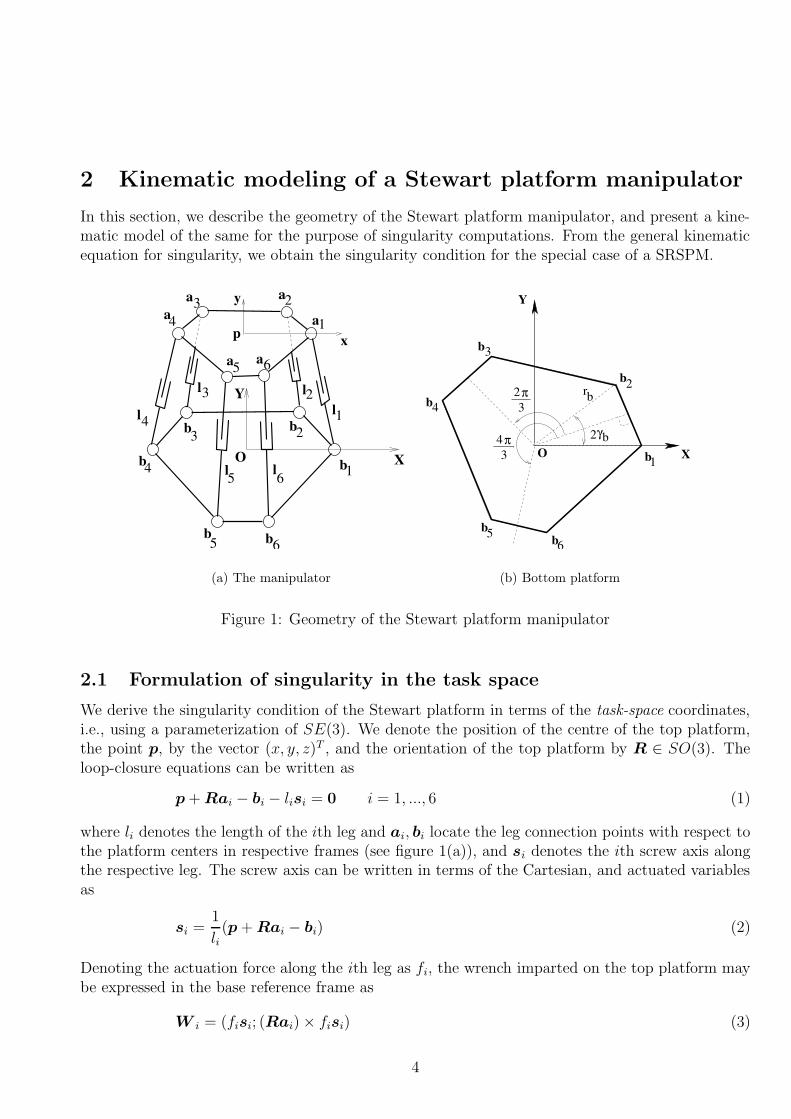
Figure 1: Geometry of the Stewart platform manipulator

2.1 Formulation of singularity in the task space

We derive the singularity condition of the Stewart platform in terms of the task-space coordinates,i.e., using a parameterization of SE(3). We denote the position of the centre of the top platform,the point p, by the vector (x, y, z)T , and the orientation of the top platform by R ∈ SO(3). Theloop-closure equations can be written as

p+Rai − bi − lisi = 0 i = 1, ..., 6 (1)

where li denotes the length of the ith leg and ai, bi locate the leg connection points with respect tothe platform centers in respective frames (see figure 1(a)), and si denotes the ith screw axis alongthe respective leg. The screw axis can be written in terms of the Cartesian, and actuated variablesas

si =1

li(p+Rai − bi) (2)

Denoting the actuation force along the ith leg as fi, the wrench imparted on the top platform maybe expressed in the base reference frame as

W i = (fisi; (Rai)× fisi) (3)

4

Using the expression for si from equation (2), W i may be written as

W i =

(fili

(p+Rai − bi);fili

((Rai)× (p− bi)))

(4)

Denoting the force and moment parts of the resultant wrench applied on the top platform due toall the leg forces as W =

∑6i=1W i = (F ;M), the equation for statics of the top platform may be

written as

1l1

(p+Ra1 − b1)1 . . . 1l6

(p+Ra6 − b6)11l1

(p+Ra1 − b1)2 . . . 1l6

(p+Ra6 − b6)21l1

(p+Ra1 − b1)3 . . . 1l6

(p+Ra6 − b6)31l1

((Ra1)× (p− b1))1 . . . 1l6

((Ra6)× (p− b6))11l1

((Ra1)× (p− b1))2 . . . 1l6

((Ra6)× (p− b6))21l1

((Ra1)× (p− b1))3 . . . 1l6

((Ra6)× (p− b6))3

f1

f2

f3

f4

f5

f6

=

(FM

)(5)

Equation (5) can be written compactly as

W = Hτ (6)

where τ = (f1, f2, f3, f4, f5, f6)T is the generalized leg force vector, and the 6× 6 matrix on the lefthand side of the equation is the wrench transformation matrix of the top platform, H. It may benoted that the use of equation (2) ensures that equation (6) is kinematically consistent, namely theloop closure equations are satisfied.

The wrenches lie in the column space of H for all joint forces τ . For a fully actuated non-redundant 6-degrees-of-freedom spatial manipulator, H is a 6× 6 matrix, and in a general config-uration, it is invertible. The column space of H spans se∗(3) in such a case, i.e., all the possiblewrenches W at the end-effector can be supported by the joint force vector. However, if there existsa wrench of finite magnitude in se∗(3) that can not be supported by a finite joint force vector τ ,then the left-nullspace of H, i.e., the orthogonal complement of the column space ofH with respectto se∗(3) is non-null, and W lies in that space. This implies that

DH = det(H) = 0 (7)

The singularity manifold M is defined by the equation (7). Further, from equation (5), DH maybe written as

DH =1

l1l2l3l4l5l6det

((p+Ra1 − b1)T . . . (p+Ra6 − b6)T

((Ra1)× (p− b1))T . . . ((Ra6)× (p− b6))T

)(8)

and, M, as defined in equation (7) is clearly independent of li. Hence, the singularity conditioncan be restated as

det(H1) = det

((p+Ra1 − b1)T . . . (p+Ra6 − b6)T

((Ra1)× (p− b1))T . . . ((Ra6)× (p− b6))T

)= 0 (9)

where H1 is the 6× 6 matrix on the right-hand side of the above equation.It may be noted that this form is true for all SPMs, and similar spatial parallel manipulators,

whose wrench transformation matrix is of the form of equation (5). The singularity condition fora SPM, equation (9), can be further simplified for a SRSPM by a suitable choice of a coordinatesystem and a parameterization of SO(3) and this is discussed next.

5

2.2 Geometry of the SRSPM

The SRSPM has hexagonal top and bottom platforms, with alternate sides in each platform havingidentical length. There is a 3-way symmetry in each platform, and the adjacent pairs of legs arearranged symmetrically about the three radial lines of symmetry in each platform. The angularspacings between the adjacent pairs of legs are denoted by 2γt, and 2γb for the top and bottomplatforms respectively. Without any loss of generality, the circum-radius of the bottom platform isscaled to unity2 and thereby one architectural parameter is eliminated from all subsequent compu-tations. The top circum-radius is denoted by rt.

In literature, it is a de facto convention to choose one of the three axes of symmetry in theplatforms as the local X direction. Therefore, the angular spacing of the legs (in the top platformfor instance) become γt = (−γt, γt, 2π/3 − γt, 2π/3 + γt, 4π/3 − γt, 4π/3 + γt) with respect tothe corresponding X axis. However, we choose the X axis to pass through the connection pointof the first leg in each platform, such that the spacings are given by γ t = (0, 2γt, 2π/3, 2π/3 +2γt, 4π/3, 4π/3 + 2γt), γb = (0, 2γb, 2π/3, 2π/3 + 2γb, 4π/3, 4π/3 + 2γb) respectively in the top andbottom platform. In this way, three of the leg connection points lie on the axes of symmetry, andthe arrangement results in a significant reduction of complexity in all subsequent computations.The manipulator along with the frames of reference used is shown in figure 1(a), and the bottomplatform, in figure 1(b).

With the above choice of the coordinate system, the SRSPM is described by 9 parameters:(rt, γb, γt) defining the architecture, and 6 local coordinates of SE(3) - as seen later an algebraicrepresentation of the rotation matrix is chosen using the Rodrigue’s parameters c = (c1, c2, c3)(see Appendix A for details) as this helps in symbolic computations. Therefore, the singularitymanifold, M, can be described by a hyper-surface in <9, each point of which defines one singularconfiguration3.

3 Simplification of algebraic-trigonometric expressions and

their canonical forms

In kinematic computations and in attempts to obtain closed form analytic expressions, we frequentlycome across large and complex mathematical expressions involving algebraic and trigonometricterms. The symbolic simplification of large and complex expressions is an old problem and isknown to be NP hard and the use of a computer algebra system (CAS) is necessary to simplifyand manipulate such expressions. In this section, we describe a scheme for this purpose using threecanonical forms of such expressions. We have used the scheme in conjuction with Mathematica[24]in our work to obtain compact, closed form, analytic expressions for the singularity manifold, M,of a Stewart platform manipulator.

2We use radians for the angular unit, while the length unit for base platform can be chosen as convenient. Allother lengths are non-dimensionalized.

3It may be noted that the 9 variables determine li’s via the inverse kinematics relationships and hence li’sthemselves do not influence the dimension of the M.

6

3.1 Complexity of a symbolic expression and limitations of heuristicsimplification schemes

The notion of complexity of an expression, in the domain of symbolic computation, tend to becase-specific, and therefore non-unique. Likewise, the definition of the most simplified or canonicalform of an expression is also subjective. Various practical (albeit heuristic) measures of complexityare used in CAS’s to detect possibilities of automatic simplification. One common practice is toconstruct the tree description of the expression, and use the total number of leaves or terminal nodesas a measure of complexity (e.g., the default measure used in the simplification schemes of the CASMathematica). The heuristic measures do not necessarily make use of the algebraic structure of theexpression, and are not proof against missing out certain non-trivial simplifications. Apart fromthis theoretical limitation, the practical difficulties of such simplification schemes can be forbidding.We discuss the most outstanding issues below.

• For any large and complex expression, such as det(H1) = 0, the simplification algorithms takevery long time and quickly use up all the computer memory. In the context of Mathematica,FullSimplify quickly runs out of memory and one has to compromise by using the morerudimentary Simplify. However, Simplify does not simplify completely, and we are leftwith still complex descriptions of the actual expression. Due to the incomplete simplificationof the coefficients of a polynomial, some of the actually zero coefficients may not be identifiedas zeros. This would give wrong information about the degree of the polynomial if it happensso with the leading coefficient, or report a wrong algebraic structure in general.

• It is known that a general univariate polynomial having degree greater than 4 can only besolved numerically (see, for example, [10]), and that the zeros of a polynomial can be sensitiveto the errors in the coefficients, particularly if the degree of the polynomial is high [20]. Due toaccumulation of errors in the lengthy numerical evaluation of the incompletely simplified coef-ficients, numerically obtained zeros of a high degree polynomial can be significantly erroneous.Further, the actual zeros which escape identification, can show up as small non-zero values,and corrupt the accuracy all subsequent computations. Although it is possible to increase thenumerical precision of the evaluation process almost arbitrarily within a CAS, it can only bedone at the cost of greater computational time, and inflexibility of implementation.

To overcome the problems associated with heuristic simplification schemes, we develop a deter-ministic substitute for a class of expressions involving both trigonometric and algebraic terms. Theend result of these schemes in each case is a canonical form of the input expression.

3.2 Deterministic simplification schemes using canonical forms of ex-pressions

Let E be a symbolic expression involving m algebraic variables x = (x1, x2, . . . , xm), and l trigono-metric variables γ = (γ1, γ2, . . . , γl) with the property that it can be cast as a polynomial in at leastone of the variables4. Without loss of generality, we choose the lexicographical variable order (i.e.,x1 � x2 � · · · � xm) for our discussion (see, for example, [3]).

4In the case of absence of any such variable, we have to use only trigonometric simplifications.

7

It is known in literature that multivariate polynomials over various coefficient domains, suchas <,C,Q, can have several canonical representations, such as the nested canonical form and themonomial-based canonical form (see [5, 2] for various representations of multivariate polynomials).We propose to generalize the ideas behind these representations to the case where the coefficientsare complicated expressions of trigonometric variables, and employ these concepts for simplificationof complex expressions. Apart from the above two forms, we use a combination of the these, andterm it the hybrid canonical form. The common features of all three schemes are:

• Isolation of algebraic and trigonometric variables using the algebraic structure of the expres-sion.

• Decomposition of the original expression into number of smaller terms.

• Grouping and simplification of the trigonometric subexpressions.

• Reconstruction of the original expression from simplified subexpressions.

In the following, we discuss these three forms, their merits and demerits.

3.2.1 Simplification using the nested canonical form

We explain the scheme for the case of univariate polynomials, and then generalize it to the multi-variate case. Let E be a degree n1 polynomial in x1 represented as

E =

n1∑

i=0

C1i x

n1−i1 = C1 · p1 (10)

where the power vector p1 consists of the powers of x1: p1 = (xn1

1 , xn1−11 , . . . , x1, 1) and the coefficient

vector C1 = (C10 , C

11 , . . . , C

1n1−1, C

1n1) contains the corresponding coefficients. Note that in such a

description, all the trigonometric terms appear only in the elements of the coefficient vector C1. Themajor consequence of this step is that the original expression is broken into (n1 +1) separate terms,algebraic complexities of each of which are lesser than that of E due to the absence of the variablex1. In spite of the fact that (n1 + 1) expressions have to be simplified now, the computationalcost of simplifying C1 is lesser and the final results better than simplifying E directly [2]. Thesimplification scheme for E may be written as

simplify(E) =n1+1∑

i=0

Simplify(C1i )p

1i = Simplify(C1).p1 (11)

where simplify denotes our scheme of simplification, and Simplify denotes the simplification operatorof the CAS employed. It may be noted that the coefficients can be simplified sequentially, or inparallel, as the case may be, and then put together to reproduce the original expression in asimplified form.

The gains in speed and compactness become significantly more prominent with the increase indepth of transformation of type (10), i.e., with more number of algebraic variables. We treat each

8

of C1i as our input expression now, and repeat the same procedure as above in a recursive manner.

Using the above notation, we can write

C1i =

n2i∑

j=0

C2ijx

n2i−j

2 = C2i · p2

i (12)

where p2i = (x

n2i

2 , xn2i−1

2 , . . . , x2, 1) and C2i = (C2

i0,C2i1, . . . ,C

2n2i−1,C

2n2i) is the corresponding coeffi-

cient vector, which is free of x1, x2. The integer n2i denotes the degree of C1

i in x2. At this stage,the simplified form of E would be given as

simplify(E) =

(n1∑

j=0

Simplify(C2j

)· p2

j

)· p1 (13)

A comparison of equations(11, 13) illustrates how the operator Simplify penetrates deeper into theexpressions down the coefficient tree with each algebraic variable isolated. It is important to notethat all simplifications are done only at the leaves of the coefficient tree. As a result, individual callsto the simplification routine deal with progressively smaller, and simpler expressions as we movedown the tree, and yield much faster, better results than can be obtained at the higher levels of thetree with comparable computational cost.

The process can be continued recursively, resulting in the set of vectors C3ij at the next level,

up to Cmi1i2...im−1

at the final level. These final vectors are independent of x, and contain thetrigonometric terms in γ. The coefficients of the lowest level are now subjected to the deterministictrigonometric transformations and the corresponding simplifications obtained with remarkable gainin speed and compactness. The algorithm can now trace back via compositions of the form ofequation (13), and return the final simplified expression.

As an example of nested canonical form of expressions, we cast the singularity polynomial ofequation (20) of section 4.2 in this form:

E =x2(E1z + E2) + x(y(E3z + E4) + E5z2 + E6z + E7) + y2(E8z + E9)+

y(E10z2 + E11z + E12) + E13z

3 + E14z2 + E15z + E16 (14)

We observe that the above scheme of simplification has several advantages:

• There is a great increase of speed in the simplification process. Depending on the particularstructure of E, an increase of 10 to 100 times was observed in our computations.

• The final expression is obtained in a canonical form. From the description of the schemeabove, it is apparent that we have traversed the coefficient tree for a multivariate polynomial(which is unique up to the choice of variable order) down to the leaves. The set of leaves,however, depend only on the power-products of xi’s present in E, and is therefore unique foreach expression. The leaves may consist of only algebraic expressions in constants from <,C,Qetc., and trigonometric functions of γi. We can first expand these expressions algebraically, andthen apply simplifying trigonometric transformations. Both of these steps are deterministic innature, and produce unique results for a given set of simplifying transformations. Thereforethe final expression obtained in this process is not subjected to any heuristic treatment at anystage, and has a deterministic structure. We call the multivariate polynomial with simplifiedtrigonometric coefficients as the nested canonical form of E.

9

• The returned expression is free of expressional redundancies at least as far as trigonometricterms are concerned. In a heuristic simplification scheme, such as minimization of leaf-countof the expression tree, the algebraic structure of the expression is not taken into considera-tion. Many trigonometric cancellations and/or simplifications may be overlooked as the termsconcerned appear at different nodes of the expression tree, and expanding the tree, at leaston the onset, can be unfavorable in terms of leaf count. Even the final canonical expressionneed not be the best in terms of leaf-count. However, the trigonometric terms that belong to aparticular monomial, and can therefore potentially combine according to trigonometric rules,are brought together under the same node by our scheme. It is therefore guaranteed that allpossible simplification steps are attempted for a given set of trigonometric transformationsavailable.

• The algebraic structure information (e.g., power products of all the elements of x, or any subsetthereof), can be obtained trivially from the canonical form. Further algebraic manipulationsusing the simplified expressions are greatly facilitated due to their standard form.

• One great advantage for algebraic geometry computation with the canonical form is that dueto exhaustive simplification of the coefficients, it is possible to identify the zeros among them,if any. Due to the complexity of the expressions, the zeros may not be apparent, and are easyto miss in a heuristic simplification scheme.

There are some disadvantages in using the nested form as the final expression. In general, ina multivariate polynomial, all possible power products are not present. In fact, with increasingnumber of variables, the number of missing power-products is expected to increase rapidly, as allthe children of a node corresponding to a missing power at any level can only be zeros. Since manyof these zeros can only be identified at the leaves, we can end up with a lot of redundant zerosamong them. Further, the same expression can have different coefficient trees if the variable orderis changed. Some of the orders can produce better results than the others for the same expression,and the choice of the best order is again heuristic. Primarily to overcome these problems, we studyanother standard form, known as the monomial-based canonical form.

3.2.2 Simplification using the monomial-based canonical form

In this representation, we retain the non-zero coefficients of individual power-products in explicitform, and express the polynomial as a sum of monomials in xi’s. At different levels, the expressionE can be written as

E = D1 · q1 = D2 · q2 = · · · = Dm · qm (15)

The vector qj consists of power-products of x1, x2, . . . , xj including unity, and the vector Dj consistsof the corresponding coefficients. The simplification is done at the lowest level, and the simplificationscheme can be written in analogy with equation (11) as

simplify(E) = Simplify(Dm) · qm (16)

To construct such a description, we follow the same steps as in the nested canonical form, startingwith a variable order. For the case of a single variable x1, the results are also exactly the same. For

10

the multivariate case, we construct the coefficient and power arrays in the same way as in equation(10). However, before moving to the next level, we eliminate the zero coefficients from C1. Let thenew coefficient vector be C1′, and let its size be m1. We modify the power vector p1 accordingly,and call it p1′ . The coefficients of the next level can be constructed similarly as

C1′i = C2′

i · p2′i (17)

Now, we construct the array of all power products of x1, x2 by taking the union of the arrays p′ip2′i :

q2 =m1⋃

i=0

p′ip2′i (18)

The corresponding array of coefficients, D2, can be constructed similarly, and the process canrepeat (m−1) times to give the final arrays of power products qm and coefficients Dm respectively.The elements of Dm correspond to Cm

i1i2...im−1, and are independent of x, and contains all the

trigonometric terms which can be simplified in a similar fashion. In fact, given one canonical form,it is not difficult to construct the other. However, this form offers some important advantages:

• Compactness of representation and ease of manipulation: We maintain the coefficients andthe powers-products in two vectors explicitly after eliminating all missing terms. Thereforethe representation is more compact and easy to maintain and manipulate than the previousone.

• Uniqueness of representation: Given a set of variables, the final vectors Dm and qm areinvariants as sets, and a change of variable order can only reorder them.

• Identification of trivial zeros of an equation: If we have an equation of the form E = 0, byconverting it to the monomial-based canonical form E = Dm · qm, we get all the power-products in the array qm. It is trivial to obtain the GCD of these power-products, whichcorresponds to the trivial zeros of the equation. Canceling off the GCD from qm, these trivialzeros can be eliminated, resulting in an equation of lower degree.

• Identification of special structures of an equation: It is possible for the power-products to showcertain special patterns, which can be identified trivially from the array qm. For example, inmany cases of kinematic analysis, there is symmetry of even order associated with a certainvariable, causing the variable to occur only in even powers in qm. Therefore, the square (orsome higher even power) of the variable can be replaced by another symbol, reducing thedegree of the resulting equation to half (or lesser) of the original.

An example of an expression cast in this form is the left-hand side of equation (20), where thealgebraic variables are x, y, z.

The disadvantage of the second canonical form of E becomes apparent with increasing numberof algebraic variables, as the array qm starts growing in size. It is difficult to anticipate a priori theactual size of these arrays, as the algebraic structure of E is not known in general. Therefore onecan always obtain the monomial-based canonical form as a starting point of simplification. If thearrays are found to be unacceptably large in size, we can arrive at a compromise between ease ofoperation and size by introducing another form of great practical value: the hybrid canonical form,which is discussed next.

11

3.2.3 Simplification using the hybrid canonical form

The hybrid form makes use of both the nested and the monomial-based canonical forms. In thiscase, we divide the algebraic variables x into two groups, namely primary algebraic variables, andsecondary algebraic variables. The final expression is returned in the monomial-based form in theprimary algebraic variables, while the individual coefficients are put into the nested canonical form.As an example, we write below the hybrid canonical form of the polynomial in equation (20), wherex, y are the primary variables, and z alone is the secondary variable:

E =x2(E1z + E2) + xy(E3z + E4) + y2(E8z + E9) + x(E5z2 + E6z + E7)+

+ y(E10z2 + E11z + E12) + E13z

3 + E14z2 + E15z + E16 (19)

The advantages of this canonical form are the following:

• By choosing the primary variables as the ones which are expected to be involved in furthersymbolic computations (such as elimination), we get the corresponding power-products inexplicit form, thereby making algebraic manipulations particularly simple.

• The secondary variables are often the ones that are to be evaluated, rather than manipulatedsymbolically, and subsequently merged numerically into the coefficients of the power-productsof the primary variables.

• For relatively large-sized problems, it appears much easier to look into the one sub-problem ata time, e.g., the effect of one variable on the zeros of a polynomial. The partitioning schemeof the hybrid form allows for such focused analysis (see the derivations of Sp and SO in thenext section for such examples).

For relatively large-scale problems, the hybrid canonical forms turn out to be the most suitable,and we use them extensively in this paper. We also note that after applying one or more of the abovesimplifications, the expression E can always be subjected to the standard simplification schemesbased on number of leaves minimization. It is our observation that such post-processing steps canimprove the compactness of the final expression as these steps can take advantage of the highlystructured canonical forms.

In the next section, we apply these schemes to simplify the singularity condition of the SRSPM,and reduce it to a form amenable to further analysis.

4 Singularity manifold of the SRSPM

In this section, we describe the derivation of the singularity manifold (M) of the SRSPM in closedform, and discuss its salient features. For a given architecture and orientation, the singularitymanifold is shown to reduce to a cubic surface Sp ∈ <3. A complete geometric characterization ofthe surface, and its explicit parameterization are obtained in the following discussion. Further, usingthe Rodrigue’s parameters (c1, c2, c3) to represent orientation, we show that for a given architectureand position, M reduces to a 6th degree surface SO in the local coordinates ci. Finally, using theball parameters (see Appendix A for details), we derive the set of rotation angles that lead to asingularity for a given axis of rotation.

12

4.1 Derivation of the singularity manifold

The singularity manifold M is defined by the equation (9) in section 2 and is given as DH1 =det(H1) = 0. The computation of the determinant of the 6× 6 matrix H1 presents great difficul-ties. In reference [22], the authors point out the problems of relying on the default determinantcomputation routines of a CAS, and come up with a customized procedure based on recursive cofac-tor expansions. In reference [23], the authors use a similar algorithm and report that the singularitymanifold can be obtained via a cascade of 590 coefficients for a general SPM, and in [13], the au-thors report obtaining the singularity condition via a computation of 3981 symbolic determinants.In this paper, we have done all the symbolic computations in the CAS Mathematica [24]5, and weobtain det(H1) in a non-simplified form using the default routine Det. The size of the Mathematicaexpression of the determinant is quite large, of the order 2.7 MB. However, we are able to simplifythe same using the procedures described in section 3.

The algebraic variables appearing in det(H1) are x = (rt, c1, c2, c3, x, y, z) and the trigonometricvariables are γ = (γb, γt). However, det(H1) is a rational function in ci due to the parameterizationof R used (see equation (40) in Appendix A), and we need to rationalize it first in order to use oursimplification schemes. Noting that the only denominator in R (and in det(H1)) is (1+c2

1 +c22 +c2

3),we replace it by a dummy variable c0, and multiply H1 by c0 to get rid of all denominators. Wenow study the algebraic structure of det(c0H1) using the monomial-based canonical form, and findthat it is of degree 6 in ci, and degree 3 in x, y, z, and degree 6 in rt. To isolate the orientationparameters, we construct next the hybrid canonical form with rt, x, y, z as primary variables, andc1, c2, c3, c0 as secondary variables. This results in a coefficient array of 71 elements, whose totalsize is about 324 MB in the non-simplified form. After simplification, only 24 non-zero coefficientsremain, while the rest are identified as zero. Further, from the power vector, it is possible to identifythe common factor r3

t among its elements, which is canceled off subsequently (rt can not be zero fora top platform of non-zero dimension). Similarly, the coefficients have c0 as their common factor,which is also canceled off, as c0 being a sum of squares of real numbers, can never be zero. Next,we substitute the actual expression of c0 into the coefficients, and simplify each of these to theirmonomial-based canonical forms with respect to the variables c1, c2, c3. These steps reduce the sizeof the coefficient vector drastically from 324 MB to about 1MB, though no further cancellationof non-zero factors can be performed at the last stage. Since all the trigonometric simplificationsare complete in a deterministic sense at this stage, we use the heuristic Simplify command ofMathematica. This results in another remarkable contraction of the coefficients, bringing themdown to about 45 KB which is approximately one page of Mathematica textual output. It is alsopossible to recognize the common factor 27

4(1 + c2

1 + c22 + c2

3)3 among the simplified coefficients atthis stage, which we cancel off. The singularity condition, i.e., the equation forM is now obtainedin terms all the manipulator parameters in a simplified form. The split of algebraic variablesnow needs to be changed for constructing the two singularity surfaces. In particular, to defineSp, the singularity condition is reconstructed in the hybrid form, with only x, y, z as the primaryvariables, and rt, c1, c2, c3 as the secondary variables. After simplification, this final form reducesto 16 monomials, whose coefficients take only about 43 KB in Mathematica. The highest degreeof these monomials is found to be 3. Similarly, to construct SO, we construct the hybrid canonicalform with only c1, c2, c3 as the primary variables, resulting in a 6th degree polynomial, with 77

5We have used Mathematica version 5.1 for 64 bit Linux (x86 64) on a PC with a single AMD Athlon 3200+processor running at 2.0 GHz, and 2 GB of RAM.

13

monomials, having a total size of about 165 KB.It is therefore obvious that further manipulation, and solution of equation (9) would be much

easier in terms of the position variables, than in terms of ci, i.e., the description of Sp would bemuch simpler than that of SO.

In the following, we explain discuss the properties of Sp and SO respectively.

4.2 The singularity surface in the Cartesian space

As discussed above, the singularity condition in equation (9) can be reduced to the following poly-nomial equation for a given set of architectural parameters rt, γb, γt and orientation parametersci:

Sp ,E1x2z + E2x

2 + E3xyz + E4xy + E5xz2 + E6xz + E7x+ E8y

2z + E9y2 + E10yz

2+

E11yz + E12y + E13z3 + E14z

2 + E15z + E16 = 0 (20)

The Ei’s are the simplified coefficients of the nested canonical form in the algebraic variables(rt, c1, c2, c3)and in trigonometric variables γb, γt. The Stewart platform is in a singular configuration if the co-ordinates of the center of the top platform, (x, y, z), satisfy the above equation.

4.2.1 Comparison with existing results

Equation (20) is similar to those presented in [22, 12, 17, 23, 13], but is not exactly the same. Inparticular, the degree of the singularity expression in [22] is 4, with 32 monomials. In [12], theexpression is much tighter, with 20 monomials, and degree 3 for the general case. In the case of theSRSPM, we show above that 4 of these monomials (in particular, x3, x2y, xy2, y3) vanish, resultingin an expression that is cubic in z alone, and quadratic in x, y. The least number of monomials ispresented in [17], where the expression of the determinant of inverse Jacobian has two monomials(x2z, y2z) less than what we have in equation (20). The variation in the reported algebraic structureof the singularity condition can be attributed mainly to the following facts:

• Frames of reference and the structure of the SPM’s considered in these works are not identi-cal. As the authors point out in [22], some of their coefficients vanish in different frames ofreference. In [23], the authors discuss the algebraic structure of the singularity equation forvarious SPM structures and point out which terms vanish for different architectures.

• In the above works, the final singularity expressions are obtained via a sequence of steps, andtherefore it is quite possible that some actual zero coefficients are not identified as zeros dueto incomplete simplification in the intermediate steps. This fact is apparent in the higherdegree of the equation reported in [22] than in others.

In [23], from Table 1, the singularity manifold for an SRSPM is defined as polynomial which iscubic in z and quadratic in x and y. After removing the cubic terms x3, x2y, xy2, y3 in theirgeneral equation the number of coefficients in the polynomial matches with our result. However,the explicit coefficients are not derived (and the further simplification to the family of hyperbolas,with its degeneracy to parabola and straight lines is not carried out) in [23] (see Section 4.2.2 fordetails). The closest geometric result, to the best of our knowledge, is given by [21] where the

14

authors have shown that the singularity manifold of a planar three-degree-of-freedom manipulatorconsists of various conic sections, including ellipse, hyperbola and parabola.

In this paper, we have derived Ei ’s explicitly in terms of the architecture, and orientationparameters, and we obtain compact closed form expressions for the coefficients. To illustrate thethe compactness of the final forms of these expressions, we write below the coefficients of z3, z2, andz respectively:

E13 =8(c1

2 + c22 − c3

2 − 1) (c1

2 + c22 + c3

2 + 1)

sin3(γ)((c3

2 − 1)

cos(γ)− 2c3 sin(γ))

E14 =8(c12 + c2

2 − c32 − 1)rt sin(γ + 3γt)((c3c1

3 − 3c2c12 − 3c2

2c3c1 + c23) cos(γ + 3γt)+

(c13 + 3c2c3c1

2 − 3c22c1 − c2

3c3) sin(γ + 3γt)) sin2(γ) + 8(c12 + c2

2 + c32 + 1) sin(2γ + 3γt)

((c3c13 + 3c2c1

2 − 3c22c3c1 − c2

3) cos(2γ + 3γt)− (c13 − 3c2c3c1

2 − 3c22c1 + c2

3c3)×sin(2γ + 3γt)) sin2(γ) (21)

E15 =− 8(c12 + c2

2)(c12 + c2

2 − c32 − 1)rt

2 sin(γ)((c32 − 1) cos(γ)− 2c3 sin(γ)) sin2(γ + 3γt)+

8(c12 + c2

2)(c12 + c2

2 + c32 + 1) sin(γ)((c3

2 − 1) cos(γ)− 2c3 sin(γ)) sin2(2γ + 3γt)+

(c12 + c2

2)rt(−4c33 + 4(c3

2 − 1) cos(4γ)c3 + 4c3 − 2(c32 + 1)2 sin(2γ)+

4 cos(6γt)((c32 − 1) cos(γ)− 2c3 sin(γ))2(sin(2γ)− sin(4γ)) + (3c3

4 − 2c32 + 3) sin(4γ)+

8(2 cos(2γ) + 1) sin2(γ)(− cos(γ)c32 + 2 sin(γ)c3 + cos(γ))2 sin(6γt))

where γ = γb − γt. It can be noted that the explicit functional dependence of the coefficients iseasily seen in the above expressions.

Some existing results in singularity of the SRSPM can be readily obtained from these expressions:

• Architecture singularity [14]: It can be seen that E13, E14 and E15 vanish when sin γ = 0,i.e., γb = γt, and the two platforms are similar. Indeed, all Ei ’s vanish under this condition.Therefore the manipulator is singular at all possible configurations, i.e., it is architecturallysingular.

• Fichter’s singularity [4]: When the top platform is horizontal, we have c1 = c2 = 0, c3 =tan(θz/2), θz ∈ [0, 2π] being the rotation about the vertical axis. Upon substituting theseconditions, all Ei ’s vanish except E13, and from equations (20,21), we have

8(c23 + 1)2 sin3(γ)((1− c2

3) cos(γ) + 2c3 sin(γ))z3 = 0 (22)

Ignoring the possibilities of architectural singularity(γ = 0) and the coplanarity of the twoplatforms (z = 0), the only real solution of equation (22) is θz = γ ± π/2. The top platformis aligned with the bottom when θz = γ, therefore θz = γ± π/2 implies that the top platformis rotated by ±π/2 with respect to the bottom about the vertical axis, which is the singularconfiguration reported by Fichter.

4.2.2 Geometric characterization of the singularity surface SpEquation (20) describes the singularity surface Sp for a given set of architectural parameters rt, γb, γt,and a given orientation c1, c2, c3. We observe that Sp is cubic in z and quadratic in x, y. Therefore,absorbing the z-terms into the coefficients of power-products of x, y, we can re-write equation (20)as

C , ax2 + 2hxy + by2 + 2gx+ 2fy + c = 0 (23)

15

Equation (23) implies that each z-section of Sp is a conic section. The coefficients of the standardform of the conic section, namely a, b, h, g, f , and c, were expressed in terms of Ei, z. It is well knownthat all the properties of a conic section can be derived in terms of the coefficients a, b, h, g, f , andc. Most importantly, we can associate a function δ = h2 − ab with the conic section C, and notethat C defines an ellipse if δ < 0, a parabola if δ = 0, and a hyperbola if δ > 0 respectively. Castingδ as a polynomial in z, we find that δ is a quadratic of the form:

δ = e0z2 + e1z + e2 (24)

The sign of δ depends on the value of the discriminant ∆ = e21 − 4e0e2. Simplifying to the nested

canonical form with respect to rt, x, y, it is observed that ∆ is zero identically. Therefore, δ is aperfect square of the form

δ = (z − zp)2, zp = − e1

2e0(25)

The above equation implies that δ ≥ 0, and hence C can not be an ellipse at any section. Inparticular, it is a hyperbola in each horizontal section, apart from a unique section at z = zp whereit is a parabola. Expression of zp is given in terms of the manipulator parameters as:

zp =((1 + c23)rt sin(γ + 3γt)(−c3

1 + 3c1c22 − 3c2

1c2c3 + c32c3) cos(γ + 3γt)+

(−3c21c2 + c3

2 + c31c3 − 3c1c

22c3) sin(γ + 3γt))/(

sin(γ)(c21 + c2

2)(1 + c21 + c2

2 + c23)(2c3 cos(γ) + (c2

3 − 1) sin(γ)))

(26)

We can also conclude that the curve C, and hence the surface Sp is unbounded.It is also possible for the hyperbolas to degenerate to a pair of straight lines. Since all the Ei’s are

differentiable functions, the surface Sp is smooth and extends infinitely in the Z direction, the onlypossibility of such degeneracy is when the hyperbola gradually deforms into its asymptotes, andcontinue to deform to reappear as a hyperbola that is conjugate to the one prior to the degeneracy.The condition for this is given by:

det

a h gh b fg f c

= 0 (27)

Expanding the determinant, we cast it as polynomial in z, and it turns out to be a quintic:

f0z5l + f1z

4l + f2z

3l + f3z

2l + f4zl + f5 = 0 (28)

Simplifying fi to the nested polynomial form in rt, and ci, we find that f0 = 0, i.e., equation (28)is a quartic in reality. It is still difficult to obtain the number of real solutions for zl due to thecomplexity of fi. However, we conclude the following: Sp can degenerate into a pair of straight in0, 2 or 4 planes defined by z = zl. In these sections alone the two sheets of Sp meet at a point, asmajor axis of the hyperbolas change from X to Y or vice-versa.

It may be noted that this geometric characterization is possible due to the compact nature ofthe coefficients, Ei’s and use of the simplification algorithms described in section 3. In particular,the simplification of ∆, f0 to zero demonstrates a situation where such computations help revealthe true algebraic structure of a problem, and substantiates the claims made in section 3 about theutility of our simplification algorithms.

Consequences of this geometric characterization are as follows:

16

• It is possible to obtain an algebraic parameterization of Sp. Apart from the sections z = zp orz = zl, the surface cuts each z-plane in a hyperbola. Choosing one parameter as z, it remainsto parameterize the hyperbolas in each z plane. The hyperbolas can first be transformed intotheir canonical forms via a rotation and translation of their individual planes. The center ofC is given by

x0 =bg − fhh2 − ab

y0 =gh− afh2 − ab (29)

and the orientation of the axes of the hyperbolas in the global frame can be given by

θc = atan2(a− b, 2h) (30)

where atan2(x, y) is the two-argument inverse tangent function. In the canonical form, assum-ing X as the major axis, hyperbolas admit the parameterization x = a′

2(t + 1

t), y = b′

2(t − 1

t)

for the part on the right of the origin, and x = − a′2

(t+ 1t), y = − b′

2(t− 1

t) for the other. The

constants a′, b′ can be obtained from the coefficients in equation (23). The curves approachtheir asymptotes as t → 0, and cut the major axis when t = 1. We define a bounding boxin each plane, whose length is given by sa′ along the major axis, where s > 1 can be chosenas per convenience of visualization. Accordingly, the parameter t varies from s−

√s2 − 1 to

s+√s2 − 1. A similar parameterization can be obtained when Y is the major axis. Therefore

the pair (z, t) forms an explicit 2-parameter description of Sp.

• Topology of the nonsingular subspace of <3 at a given architecture and orientation can becomplicated, and possibly vary from case to case. For example, the central portion of thehyperbolas, containing (x0, y0) in each plane, collapses to a point at each section the hyperbolasdegenerate to a pair of intersecting straight lines. As the hyperbolas extend to infinity, eachof these portions are separated from the rest of <3 by the singularity manifold. However, asexplained above, the number of such sections can be 0, 2 or 4, and further, some of thesesections may not be realizable in a physical sense (e.g., if the section is not between the twoplatforms, such that zl < 0 in our case). Moreover, there is a single plane z = zp, in which oneof the parts of the hyperbola transforms into a parabola, while the other vanishes, therebyproviding a corridor connecting the two subspaces of <3 otherwise separated by it. Variouscombinations of the feasible (i.e., positive) values of zp and zl lead to different topologies ofthe non-singular subspaces.

It is also possible to identify certain horizontal planes where the coefficients of C show somemore special properties. We list some of them below:

• a+ b = 0 (Rectangular hyperbola):

z =rt(1 + c23) sin(γ + 3γt)((−3c2

1c2 + c32 + c3

1c3 − 3c1c22c3) cos(γ + 3γt)+

(c31 + (−3c1c

22 + 3c2

1c2c3 − c32c3) sin(γ + 3γt))/ (31)

(sin(γ)(c21 + c2

2)(1 + c21 + c2

2 + c23)((c2

3 − 1) cos(γ)− 2c3 sin(γ)))

17

• a = b (θc = π2, the global Y axis is the major axis of the hyperbola):

z =(c21 + c2

2)rt sin(γ + 3γt)((c2 − 3c2c23 + c1c3(−3 + c2

3)) cos(γ + 3γt)+

(c2c3(−3 + c23) + c1(−1 + 3c2

3)) sin(γ + 3γt))/ (32)

(sin(γ)(1 + c23)(1 + c2

1 + c22 + c2

3)((c21 − c2

2) cos(γ)− 2c1c2 sin(γ)))

• h = 0 (θc = 0, the global X axis is the major axis of the hyperbola):

z =rt(c21 + c2

2) sin(γ + 3γt)((c1 − 3c1c23 − c2c3(c2

3 − 3)) cos(γ + 3γt)+

(c2 − 3c2c23 + c1c3(c2

3 − 3)) sin(γ + 3γt))/ (33)

(sin(γ)(1 + c23)(1 + c2

1 + c22 + c2

3)(2c1c2 cos(γ) + (c21 − c2

2) sin(γ)))

4.3 Singularity surface in the orientation parameters

We now describe a complimentary representation of M, which is a surface in the local coordinatesof SO(3) for a given architecture and position. The surface, denoted by SO, is such that every pointon it corresponds to an orientation which is singular, and for a given architecture and position, allsuch orientations lie on this surface. We note that this representation ofM is not studied very welland the closest work is by Li et al. [13] where a numerical example is presented.

We start by recollecting the equation defining SO which was obtained as a polynomial consistingof 77 monomials in ci, including the constant term. The corresponding coefficients are functions ofthe architecture and position parameters of the manipulator. The highest exponents in terms of ciare 5, 5, and 6 respectively, and the total degree of the corresponding equation in ci is 6. Moreover,although ci provides a very effective means to derive SO in closed form, it is difficult to visualizethe singularities in terms of these parameters due to the following reasons:

• For a given axis of rotation (with the sense associated), the rotation can vary from 0 to π,and therefore ci can vary from −∞ to ∞. Such infinite range of values make it inappropriatefor visualization purposes.

• From a given set of ci, it is difficult to obtain an intuitive idea of the orientation, unless it isconverted to some parameter set with more apparent geometric significance.

To overcome these short-comings simultaneously, we convert the polynomial in ci to an equivalentexpression in the ball parameters via equation (43) (see Appendix A.2). Writing tθ for tan(θ/2),we obtain a 6-degree polynomial in tθ as follows:

g0t6θ + g1t

5θ + g2t

4θ + g3t

3θ + g4t

2θ + g5tθ + g6 = 0 (34)

where θ is the rotation about the axis of the finite rotation.The set of coefficients gi have an one-to-one correspondence with the unit vectors emanating

from the origin of <3. Therefore each such set represents a unique direction and the sense of rotation,and each solution of equation (34) such that tθ ∈ [0,∞], gives the corresponding angle of CCWrotation via the transformation

θ = 2 atan2(1 + t2θ, 2tθ) (35)

18

The expressions of gi’s are complicated, hence the number of feasible roots of equation (34) cannot be ascertained a priori. We can only conclude that for a given architecture and position, thereare 0, 2, 4 or 6 CCW rotations in [0, π] about any given axis such that the resulting orientation ofthe top platform leads to a singular configuration. However, these rotation angles can be computedrelatively easily using the analytical expressions of gi. Moreover, as the rotation axis is made tosweep through the entire sphere S2 (i.e., α ∈ [−π/2, π/2], β ∈ [0, 2π]), and corresponding feasiblevalues of θ are obtained, all the singular orientations can be enlisted.

It may be mentioned that the computation of orientation singularity manifold in [13] is in termsof tangent half-angles of the Euler angles. The general expressions are in terms of 3981 determinantswhich lead to 2173 coefficients, whereas our gi’s are in a much more simpler, explicit functional form.We present the expressions for g4, g5 and g6 to illustrate this.

g4 = z(4z2 cos(γ) sin2(α) sin3(γ) + 4z cos(α) sin(α)(sin(β)(y cos(γ) + 5x sin(γ))

+ cos(β)(x cos(γ)− 5y sin(γ))) sin3(γ) + cos2(α)(−4 cos(3(γ + 2γt))

× cos2(γ) + cos(γ) + 3 cos(3γ) + 4 sin(γ)(y sin(2β − γ − 3γt)− x cos(2β − γ − 3γt)) sin(γ + 3γt))

×rt sin(γ)− 2 cos2(α) sin(2γ) sin2(γ + 3γt)r2t + cos2(α)(8y2 cos(β) cos(β + γ) sin3(γ)

+8x2 sin(β) sin(β + γ) sin3(γ)− 8xy sin(2β + γ) sin3(γ)

−4x cos(2β − 2γ − 3γt) sin(2γ + 3γt) sin2(γ) + 4y sin(2β − 2γ − 3γt) sin(2γ + 3γt) sin2(γ)

−2 sin(2γ) sin2(2γ + 3γt)))

g5 = 4z2 sin3(γ)(2z sin(α) sin(γ) + cos(α)(cos(β)(x sin(γ)− 3y cos(γ))

+ sin(β)(3x cos(γ) + y sin(γ))))

g6 = 4z3 cos(γ) sin3(γ) (36)

As in the case of Sp, we observe that for two similar platforms with γ = 0 (γb = γt), g4, g5

and g6 are zero. Indeed, all gi ’s vanish under this condition, and the manipulator is singular at allpossible configurations, i.e., it is architecturally singular.

4.4 Illustrative examples

In this section, we plot the surfaces Sp and SO for a SRSPM to illustrate the results describedabove. The geometry of the top and bottom platforms are taken to be the same as the INRIAprototype [22, 23, 13]. However, the top platform is mobile in our case, and all the lengths arescaled such that the radius of the bottom platform is unity. The resulting architectural parametersof this manipulator are as follows:

rt = 0.5803, γb = 0.2985rad, γt = 0.6573rad

and therefore γ = −0.3588rad. The manipulator is shown in figure 2 below in a reference config-uration, where x = y = 0, z = 1, and R = Rz(γ), such that the axes of symmetry in the twoplatforms are vertically aligned. In the following, we present the surfaces Sp and SO respectivelyfor this manipulator.

4.4.1 Examples of SpWe choose two different orientations to illustrate Sp. First we take c1 = 0.4, c2 = 0.2, c3 =0.6. A part of the corresponding surface is shown in figure 3. For this case, zp = 0.4026,

19

Figure 2: The SRSPM in a reference configuration

Figure 3: Sp for c1 = 0.4, c2 = 0.2, c3 = 0.6

20

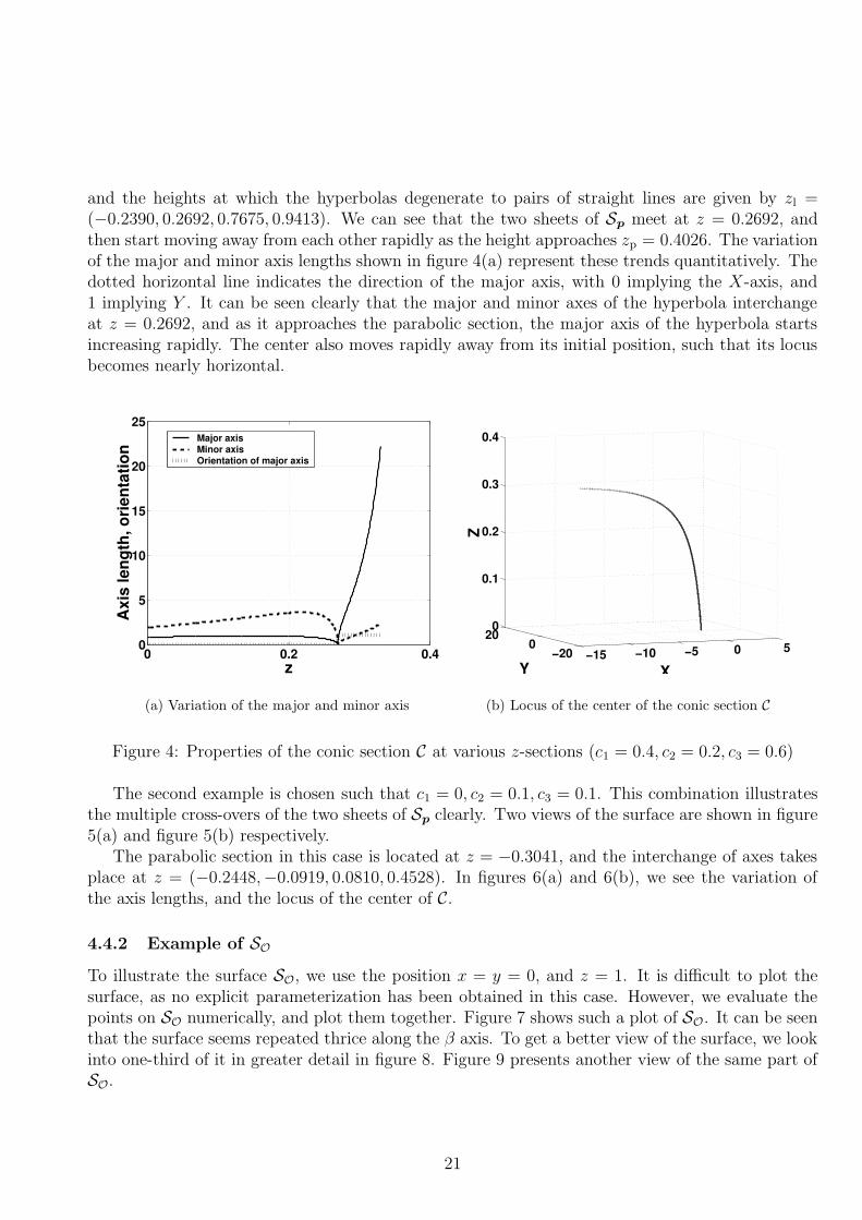
and the heights at which the hyperbolas degenerate to pairs of straight lines are given by zl =(−0.2390, 0.2692, 0.7675, 0.9413). We can see that the two sheets of Sp meet at z = 0.2692, andthen start moving away from each other rapidly as the height approaches zp = 0.4026. The variationof the major and minor axis lengths shown in figure 4(a) represent these trends quantitatively. Thedotted horizontal line indicates the direction of the major axis, with 0 implying the X-axis, and1 implying Y . It can be seen clearly that the major and minor axes of the hyperbola interchangeat z = 0.2692, and as it approaches the parabolic section, the major axis of the hyperbola startsincreasing rapidly. The center also moves rapidly away from its initial position, such that its locusbecomes nearly horizontal.

0 0.2 0.40

5

10

15

20

25

z

Axi

s le

ngth

, ori

enta

tion

Major axis Minor axis Orientation of major axis

(a) Variation of the major and minor axis

−15 −10 −5 0 5−200

200

0.1

0.2

0.3

0.4

XY

Z

(b) Locus of the center of the conic section C

Figure 4: Properties of the conic section C at various z-sections (c1 = 0.4, c2 = 0.2, c3 = 0.6)

The second example is chosen such that c1 = 0, c2 = 0.1, c3 = 0.1. This combination illustratesthe multiple cross-overs of the two sheets of Sp clearly. Two views of the surface are shown in figure5(a) and figure 5(b) respectively.

The parabolic section in this case is located at z = −0.3041, and the interchange of axes takesplace at z = (−0.2448,−0.0919, 0.0810, 0.4528). In figures 6(a) and 6(b), we see the variation ofthe axis lengths, and the locus of the center of C.

4.4.2 Example of SOTo illustrate the surface SO, we use the position x = y = 0, and z = 1. It is difficult to plot thesurface, as no explicit parameterization has been obtained in this case. However, we evaluate thepoints on SO numerically, and plot them together. Figure 7 shows such a plot of SO. It can be seenthat the surface seems repeated thrice along the β axis. To get a better view of the surface, we lookinto one-third of it in greater detail in figure 8. Figure 9 presents another view of the same part ofSO.

21

(a) View 1

(b) View 2

Figure 5: Two views of Sp for c1 = 0, c2 = 0.1, c3 = 0.1

22

0 0.2 0.4 0.6 0.8 10

1

2

3

4

5

z

Axi

s le

ngth

, ori

enta

tion

Major axis Minor axis Orientation of major axis

(a) Variation of the major and minor axis

−10−5

0

−3−2−100

0.2

0.4

0.6

0.8

1

XYZ

(b) Locus of the center of the conic section C

Figure 6: Properties of the conic section C at various z-sections (c1 = 0, c2 = 0.1, c3 = 0.1)

−0.5

0

0.5

0

0.2

0.4

0.6

0.8

1

1.2

1.4

1.6

1.8

2

0.3

0.4

0.5

0.6

0.7

0.8

0.9

α/π

β/π

θ/π

Figure 7: A view of SO at x = y = 0, z = 1

23

−0.50

0.5

0

0.2

0.4

0.6

0.8

0.3

0.4

0.5

0.6

0.7

0.8

0.9

α/πβ/π

θ/π

Figure 8: View of a part of SO at x = y = 0, z = 1

−0.5−0.4−0.3−0.2−0.100.10.20.30.40.50

0.2

0.4

0.6

0.8

0.3

0.4

0.5

0.6

0.7

0.8

0.9

α/π

β/π

θ/π

Figure 9: Another view of a part of SO at x = y = 0, z = 1

24

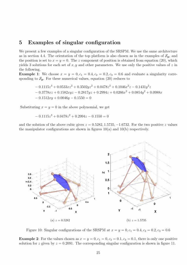
5 Examples of singular configuration

We present a few examples of a singular configuration of the SRSPM. We use the same architectureas in section 4.4. The orientation of the top platform is also chosen as in the examples of Sp, andthe position is set to x = y = 0. The z component of position is obtained from equation (20), whichyields 3 solutions for each set of x, y and other parameters. We use only the positive values of z inthe following.Example 1: We choose x = y = 0, c1 = 0.4, c2 = 0.2, c3 = 0.6 and evaluate a singularity corre-sponding to Sp. For these numerical values, equation (20) reduces to

− 0.1115z3 + 0.0533xz2 + 0.3502yz2 + 0.0478z2 + 0.1046x2z − 0.1431y2z

− 0.3778xz + 0.1582xyz − 0.2817yz + 0.2994z + 0.0266x2 + 0.0854y2 + 0.0988x

− 0.1512xy + 0.0046y − 0.1550 = 0

Substituting x = y = 0 in the above polynomial, we get

− 0.1115z3 + 0.0478z2 + 0.2994z − 0.1550 = 0

and the solution of the above cubic gives z = 0.5282, 1.5735,−1.6732. For the two positive z valuesthe manipulator configurations are shown in figures 10(a) and 10(b) respectively.

(a) z = 0.5282 (b) z = 1.5735

Figure 10: Singular configurations of the SRSPM at x = y = 0, c1 = 0.4, c2 = 0.2, c3 = 0.6

Example 2: For the values chosen as x = y = 0, c1 = 0, c2 = 0.1, c3 = 0.1, there is only one positivesolution for z given by z = 0.2091. The corresponding singular configuration is shown in figure 11.

25

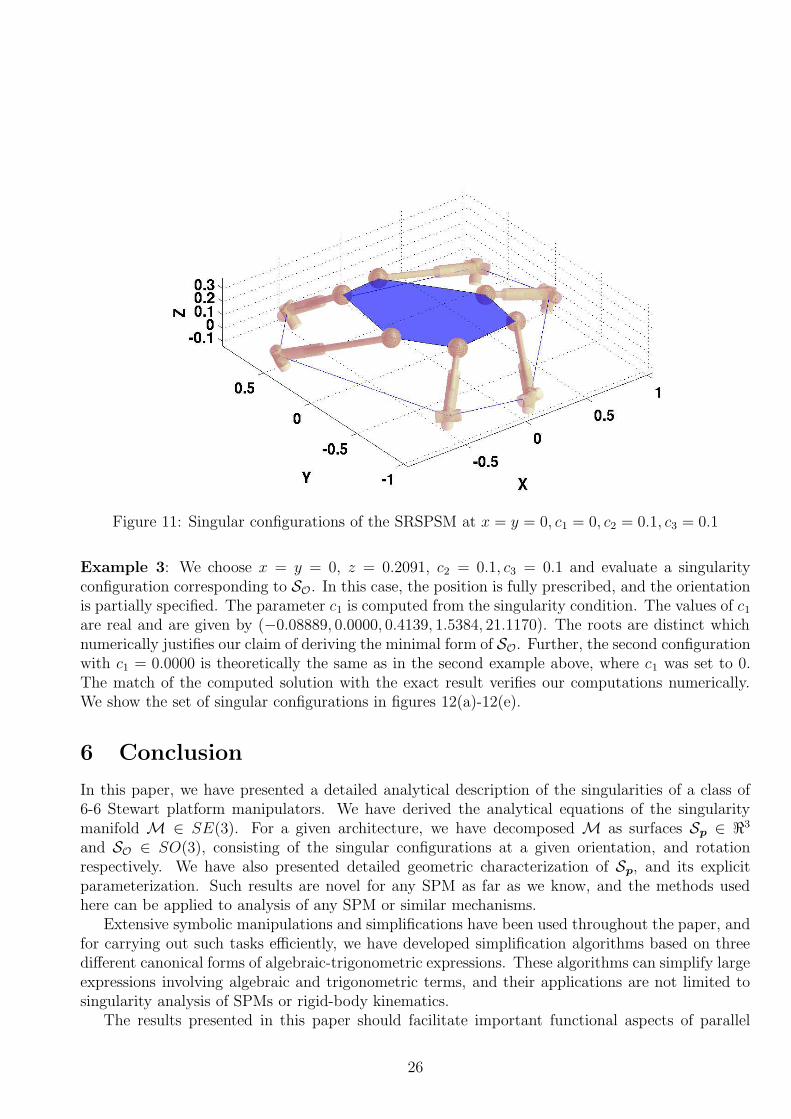
Figure 11: Singular configurations of the SRSPSM at x = y = 0, c1 = 0, c2 = 0.1, c3 = 0.1

Example 3: We choose x = y = 0, z = 0.2091, c2 = 0.1, c3 = 0.1 and evaluate a singularityconfiguration corresponding to SO. In this case, the position is fully prescribed, and the orientationis partially specified. The parameter c1 is computed from the singularity condition. The values of c1

are real and are given by (−0.08889, 0.0000, 0.4139, 1.5384, 21.1170). The roots are distinct whichnumerically justifies our claim of deriving the minimal form of SO. Further, the second configurationwith c1 = 0.0000 is theoretically the same as in the second example above, where c1 was set to 0.The match of the computed solution with the exact result verifies our computations numerically.We show the set of singular configurations in figures 12(a)-12(e).

6 Conclusion

In this paper, we have presented a detailed analytical description of the singularities of a class of6-6 Stewart platform manipulators. We have derived the analytical equations of the singularitymanifold M ∈ SE(3). For a given architecture, we have decomposed M as surfaces Sp ∈ <3

and SO ∈ SO(3), consisting of the singular configurations at a given orientation, and rotationrespectively. We have also presented detailed geometric characterization of Sp, and its explicitparameterization. Such results are novel for any SPM as far as we know, and the methods usedhere can be applied to analysis of any SPM or similar mechanisms.

Extensive symbolic manipulations and simplifications have been used throughout the paper, andfor carrying out such tasks efficiently, we have developed simplification algorithms based on threedifferent canonical forms of algebraic-trigonometric expressions. These algorithms can simplify largeexpressions involving algebraic and trigonometric terms, and their applications are not limited tosingularity analysis of SPMs or rigid-body kinematics.

The results presented in this paper should facilitate important functional aspects of parallel

26

(a) c1 = −0.0889 (b) c1 = 0.0000

(c) c1 = 0.4139 (d) c1 = 1.5384

(e) c1 = 21.1170

Figure 12: Singular configurations of the SRSPM at x = y = 0, z = 0.2091, c2 = 0.1, c3 = 0.1

27

robots, such as detection of singularities, and formal verification of trajectories. With the compactanalytical conditions for singularity allowing parametric study of designs with very less computa-tions, the task of designing singularity-free workspaces should be greatly facilitated. The methodsdescribed here can also be used without modification to study the singularities of more generalforms of the SPM.

Acknowledgement

The authors wish to thank the anonymous reviewers for their valuable comments.

References

[1] Basu, D. and Ghosal, A. (1997), ‘Singularity analysis of platform-type multi-loop spatialmechanisms’, Mechanism and Machine Theory, 32, pp. 375–389.

[2] Cohen, J. S. (2002), Computer Algebra and Symbolic Computation: Mathematical Methods, AK Peters, Natick.

[3] Cox, D., Little, J. and O’Shea, D. (1991), Ideals, Varieties, and Algorithms: An Introductionto Computational Algebraic Geometry and Commutative Algebra, Springer-Verlag, New York.

[4] Fichter, E. F. (1986), ‘A Stewart platform-based manipulator: general theory and practicalconstruction’, International Journal of Robotics Research, 5(2), pp. 157–182.

[5] Geddes, K. O., Czapor, S. R. and Labahn, G. (1992), Algorithms for Computer Algebra, KluwerAcademic Publishers, Boston.

[6] Gosselin, C. and Angeles, J. (1990), ‘Singularity analysis of closed loop kinematic chains’,IEEE Transactions on Robotics and Automation, 6(3), pp. 281–290.

[7] Gregorio, R. D. (2001a), ‘Analytic formulation of the 6-3 fully-parallel manipulators singularitydetermination’, Robotica, 19, pp. 663–667.

[8] Gregorio, R. D. (2001b), ‘Statics and singularity loci of the 3-UPU wrist’, 2001 IEEE/ASMEInternational Conference on Advanced Intelligent Mechatronics Proceedings, Italy, pp. 470–475.

[9] Gregorio, R. D. (2002), ‘Singularity-locus expression of a class of parallel mechanisms’, Robot-ica, 20, pp. 323–328.

[10] Herstein, I. N. (1975), Topics in Algebra, John Wiley & Sons, New York.

[11] Hunt, K. H. (1978), Kinematic Geometry of Mechanism, Clarendon Press, Oxford.

[12] Kim, D. and Chung, W. (1999), ‘Analytic singularity equation and analysis of six-dof par-allel manipulators using local structurization method’, IEEE Transactions on Robotics andAutomation, 15(4), pp. 612–622.

28

[13] Li, H., Gosselin, C., Richard, M. J. and St-Onge, B. M. (2004), ‘Analytic form of the six-dimensional singularity locus of the general Gough-Stewart platform’, Proceedings of ASME28th Biennial Mechanisms and Robotics Conference, Salt Lake City, Utah, USA’.

[14] Ma, O. and Angeles, J. (1991), ‘Architectural singularities of platform manipulators’, Proceed-ings of International Conference on Robotics and Automation, pp. 1542–1547.

[15] McCarthy, J. M. (2002), Geometric Design of Linkages, Springer, New York.

[16] Merlet, J.-P. (1989), ‘Singularity configurations of parallel manipulators and Grassman geom-etry’, International Journal of Robotics Research, 8, pp. 45–56.

[17] Merlet, J.-P. (2001), Parallel Robots, Kluwer Academic Press, Dordrecht.

[18] Miscehnko, A. and Fomenko, A. (1988), A Course of Differential Geometry and Topology, MirPublishers, Moscow.

[19] Murray, R. M., Li, Z. and Sastry, S. S. (1994), A Mathematical Introduction to Robotic Ma-nipulation, CRC Press, Boca Raton.

[20] Press, W. H., Teukolsky, S. A., Vetterling, W. and Flannery, B. P. (2002), Numerical Recipiesin C++: the Art of Scientific Computing, Cambridge University Press, Cambridge.

[21] Sefrioui, J. and Gosselin, C. M. (1995), ‘On the quadratic nature of the singularity curves ofplanar three-degree-of-freedom parallel manipulators’, Mechanism and Machine Theory, 30,pp. 533–551.

[22] St-Onge, B. M. and Gosselin, C. (1996), ‘Singularity analysis and representation of spatialsix-dof parallel manipulators’, Recent Advances in Robot Kinematics, pp. 389–398.

[23] St-Onge, B. M. and Gosselin, C. (2000), ‘Singularity analysis and representation of the generalGough-Stewart platform’, International Journal of Robotics Research, 19(3), pp. 271–288.

[24] Wolfram, S. (2004), The Mathematica Book, Cambridge University Press, Cambridge.

A Different parameterizations of SO(3)

In this section, we discuss the parameterizations of SO(3) used in this paper.

A.1 Rodrigue’s parameters

Rodrigue’s parameters utilizes the isomorphism between <3 and so(3), and provide an algebraicparameterization of SO(3) (see, for e.g., [15]). Using the isomorphism, we can obtain a 3 × 3skew-symmetric matrix A corresponding to a vector c = (c1, c2, c3)T as

A =

0 −c3 c2

c3 0 −c1

−c2 c1 0

(37)

29

There exists a homeomorphism from the neighborhood of 0 ∈ so(3) to a neighborhood of I 3 ∈ SO(3)due to Cayley, given by

R = (I3 −A)(I3 +A)−1 (38)

where I3 is the identity in GL3(<). Using this transformation, we can get one of the possibleexplicit formulæ for the elements of R ∈ SO(3) as

Rij =1

1 + c2k

((1− c2k + 2c2

i )δij + 2(1− δij)(cicj − ckεijk)) (39)

In matrix form, we can write

R =1

1 + c21 + c2

2 + c23

1 + c21 − c2

2 − c23 2(c1c2 − c3) 2(c1c3 + c2)

2(c1c2 + c3) 1− c21 + c2

2 − c23 2(c2c3 − c1)

2(c1c3 − c2) 2(c2c3 + c1) 1− c21 − c2

2 + c23

(40)

For any rotation matrix R. we have tr(R) = 1 + 2 cos θ, where θ ∈ [0, π] is the net rotationrepresented by R. Hence we have

1 + 2 cos θ = tr(R) =3− c2

1 − c22 − c2

3

1 + c21 + c2

2 + c23

If θ 6= 0, mπ where m is an integer, the rotation axis is well defined, and is given by the unit vectoru = (ux, uy, uz), where

2 sin θuk = Rijεijk =4ck

1 + c21 + c2

2 + c23

It can be shown that these requirements are simultaneously satisfied if we have:

c = u tan(θ/2) (41)

Equation (41) gives the geometric interpretation of ci, which are known as Rodrigue’s parameters.These parameters provide a system of local coordinates of SO(3) in the neighborhood of its identity.The major advantage of this representation of rigid-body rotation is in its algebraic nature, whichmakes its use in complicated kinematic analysis computationally economical.

A.2 Ball parameters of SO(3)

The geometric interpretation of ci leads to a 4-parameter representation of SO(3) in terms of(ux, uy, uz, θ). However, SO(3) is 3-dimensional, and this parameterization involves a constraint, i.e.,‖u‖ = 1. One can further parameterize the unit vector u to obtain a constraint free parameterizationof SO(3) as explained below.

The unit vector parallel to the rotation axis can be written as

u = (cosα cos β, cosα sin β, sinα)T (42)

where α is the angle made by u with the XY plane, and β is the angle made by the projection ofu on the XY plane with the X axis. We can now express c as

c = tan(θ/2)(cosα cos β, cosα sin β, sinα)T (43)

30

The three quantities (α, β, θ) form another local parameterization of SO(3), and are related to therepresentation of SO(3) as a ball [18]. The angles α, β serve as the latitude and longitude, whileθ ∈ [0, π] gives the radius. Each point on the surface of this ball represents a rotation uniquely.However, a given rotation corresponds to two points on the ball, which are antipodal to each other.This is because the rotation (u, θ) is equivalent to the rotation (−u,−θ) ∀θ ∈ [0, π], and it canbe shown that the ball is a doubly connected domain. The zero rotation corresponds to the center.Entire SO(3) can be covered if the axis is swept through the unit sphere S2, and the magnitudeof rotation varies from 0 to π for each such axis, i.e., α ∈ [−π/2, π/2], β ∈ [0, 2π], θ ∈ [0, π].The advantage of this parameterization over more common ones, such as the Euler angles, is thatit yields an intuitive idea of the top platform orientation directly. It can also take advantage ofthe compactness of the kinematic expressions in terms of ci via equation (43), providing geometricinsight at the same time.

31