GEOMETRIC BRST QUANTIZATION

Jose M. Figueroa-O’Farrill\

and

Takashi Kimura♣

Institute for Theoretical Physics

State University of New York at Stony Brook

Stony Brook, NY 11794-3840, U. S. A.

ABSTRACT

We formulate BRST quantization in the language of geometric quantization. We

extend the construction of the classical BRST cohomology theory to reduce not just

the Poisson algebra of smooth functions, but also any projective Poisson module

over it. This construction is then used to reduce the sections of the prequantum

line bundle. We find that certain polarizations (e.g. Kahler) induce a polarization

of the ghosts which simplifies the form of the quantum BRST operator. In this

polarization—which can always be chosen—the quantum BRST operator contains

only linear and trilinear ghost terms. We also prove a duality theorem for the

quantum BRST cohomology.

\ e-mail: figueroa@sunysbnp.BITNET, jmf@noether.UUCP

♣ e-mail: kimura@sunysbnp.BITNET, kimura@noether.UUCP

§1 INTRODUCTION

Despite the fact that the BRST method made its first appearance as an acciden-

tal symmetry of the “quantum” action in perturbative lagrangian field theory[1],[2]

it soon became apparent that it took its simplest and most elegant form in the

hamiltonian formulation of gauge theories[3], where it is used in the homologi-

cal reduction of the Poisson algebra of smooth functions of a symplectic manifold

on which one has defined a set of first class constraints. Indeed, at a more ab-

stract level, the BRST construction finds its most general form in the theory of

“constrained” Poisson algebras[4],[5]; although it is that more concrete realization

which is physically relevant, and hence the one we shall study in this paper.

The motivation behind this paper is the desire to define a quantization proce-

dure which would exploit the naturality of the BRST construction in the symplectic

context. Geometric quantization[6] is just such a quantization procedure, since it

can be defined purely in terms of symplectic data and hence seems tailored for this

purpose.

The problem of defining a BRST quantization procedure has been recently

analyzed in the literature[7]. In [7] the authors discuss the BRST quantization in

the case of constraints arising from the action of an algebra and they focus only on

the ghost part assuming that the quantization of the ghost and matter parts are

independent. In this paper we show that this is not always the case in geometric

quantization, since the polarization of the matter forces, in some cases, a particular

polarization of the ghosts. Also general properties of BRST quantized theories have

recently been studied in [8] in the context of Fock space representations and in [9]

in a slightly more general context. See also the recent paper [10] .

The organization of this paper is as follows. In Section 2 we review the sym-

plectic reduction of a symplectic manifold (M,Ω) by a coisotropic submanifold Mo.

This material is standard in the mathematics literature and thus we only mention

the main facts. We remark that symplectic reduction, as well as cohomology, is a

basically a subquotient. This becomes the dominant theme of the paper.

– 2 –

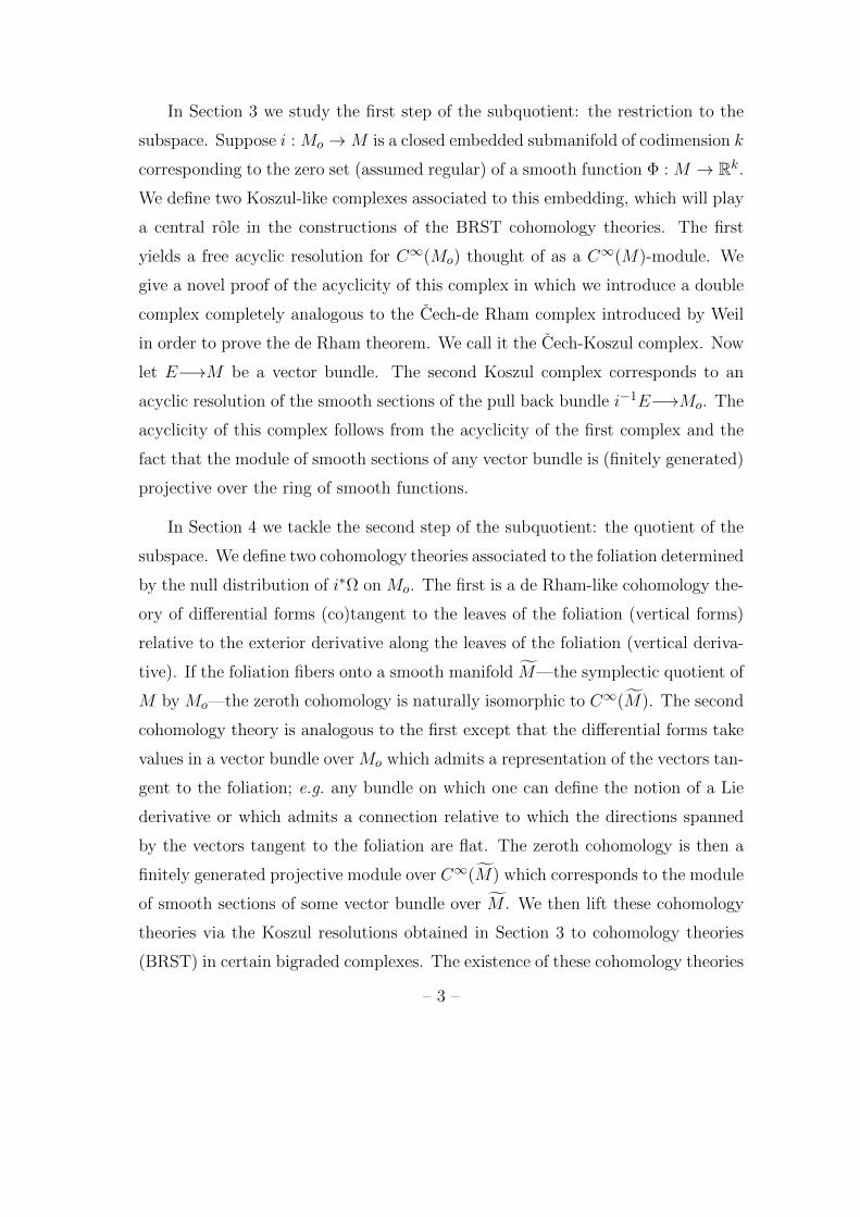
In Section 3 we study the first step of the subquotient: the restriction to the

subspace. Suppose i : Mo →M is a closed embedded submanifold of codimension k

corresponding to the zero set (assumed regular) of a smooth function Φ : M → Rk.

We define two Koszul-like complexes associated to this embedding, which will play

a central role in the constructions of the BRST cohomology theories. The first

yields a free acyclic resolution for C∞(Mo) thought of as a C∞(M)-module. We

give a novel proof of the acyclicity of this complex in which we introduce a double

complex completely analogous to the Cech-de Rham complex introduced by Weil

in order to prove the de Rham theorem. We call it the Cech-Koszul complex. Now

let E−→M be a vector bundle. The second Koszul complex corresponds to an

acyclic resolution of the smooth sections of the pull back bundle i−1E−→Mo. The

acyclicity of this complex follows from the acyclicity of the first complex and the

fact that the module of smooth sections of any vector bundle is (finitely generated)

projective over the ring of smooth functions.

In Section 4 we tackle the second step of the subquotient: the quotient of the

subspace. We define two cohomology theories associated to the foliation determined

by the null distribution of i∗Ω on Mo. The first is a de Rham-like cohomology the-

ory of differential forms (co)tangent to the leaves of the foliation (vertical forms)

relative to the exterior derivative along the leaves of the foliation (vertical deriva-

tive). If the foliation fibers onto a smooth manifold M—the symplectic quotient of

M by Mo—the zeroth cohomology is naturally isomorphic to C∞(M). The second

cohomology theory is analogous to the first except that the differential forms take

values in a vector bundle over Mo which admits a representation of the vectors tan-

gent to the foliation; e.g. any bundle on which one can define the notion of a Lie

derivative or which admits a connection relative to which the directions spanned

by the vectors tangent to the foliation are flat. The zeroth cohomology is then a

finitely generated projective module over C∞(M) which corresponds to the module

of smooth sections of some vector bundle over M . We then lift these cohomology

theories via the Koszul resolutions obtained in Section 3 to cohomology theories

(BRST) in certain bigraded complexes. The existence of these cohomology theories

– 3 –

must be proven since the vertical derivative does not lift to a differential operator,

i.e. its square is not zero. However its square is chain homotopic to zero (relative

to the Koszul differential) and the acyclicity of the Koszul resolution allows us to

construct the desired differential.

In Section 5 we review the basics of Poisson superalgebras and define the notion

of a Poisson module. We have not seen Poisson modules defined anywhere but we

feel our definition is the natural one. We then show that the BRST cohomologies

constructed in Section 4 are naturally expressed in the context of Poisson super-

algebras and Poisson modules. This allows us to prove that not only the ring and

module structures are preserved under BRST cohomology but, more importantly,

the Poisson structures also correspond.

We are then ready to begin applying the constructions of the previous sections

to the geometric quantization program. We have divided this into two sections: one

discussing prequantization and the other polarization. In Section 6 we discuss how

prequantum data is induced via symplectic reduction. If (M,Ω) is prequantizable

then there is a hermitian line bundle with compatible connection such that its

curvature is given by −2π√−1Ω. Its pull back onto Mo is also a hermitian line

bundle with compatible connection whose curvature is −2π√−1i∗Ω. Since the

flat directions of this connection coincide with the directions tangent to the null

foliation, the smooth sections of this line bundle admit a representation of the

vector fields tangent to the foliations and thus we can build a BRST cohomology

theory as in Sections 4 and 5. We prove that all the prequantum data gets induced

a la BRST except for the inner product, which involves integration. We discuss

the reasons why.

In Section 7 we discuss how to induce polarizations. We find that in many

cases—pseudo-Kahler polarizations, G action with G semisimple—a choice of po-

larization for M forces a polarization of the ghost part. This is to be compared

with [7] where the quantization of the ghost and the matter parts are done sep-

arately. In particular one can always choose a polarization for the ghost part in

– 4 –

which the quantum BRST operator simplifies enormously since it only contains

linear and trilinear ghost terms.

In Section 8 and modulo some minor technicalities which we discuss there,

we prove a duality theorem for the quantum BRST cohomology. Some of the

technicalities are connected to the potential infinite dimensionality of the spaces

involved.

Finally in Section 9 we conclude by discussing some of the results and some

open problems.

Note added: After completion of this work we became aware of the paper by

Johannes Huebschmann [11] where he discusses geometric quantization from an

algebraic stand point. He identifies Poisson algebras as a special kind of Rinehart’s

(A,R)–algebras. Under this identification our notion of Poisson module agrees with

his. He also treats reduction but not in its more general case and without using

BRST. In this purely algebraic context reduction can be taking into account by

an algebraic extension of BRST a la Stasheff. We are currently investigating this

extension. We wish to thank Jim Stasheff for making us aware of this work and

Johannes Huebschmann for sending us the preprint.

§2 SYMPLECTIC REDUCTION

In this section we review the reduction of a symplectic manifold by a coisotropic

submanifold. In particular we are interested in the case where the submanifold is

the zero locus of a set of first class constraints. The interested reader can consult

[12] for a very readable exposition of this subject.

Let (M,Ω) be a 2n-dimensional symplectic manifold and i : Mo → M a

coisotropic submanifold. That is, for all m ∈ Mo, TmM⊥o ⊆ TmMo, where

TmM⊥o = X ∈ TmM | Ω(X, Y ) = 0 ∀Y ∈ TmMo. Because dΩ = 0, the

distribution m 7→ TmM⊥o is involutive and it is known as the characteristic or null

distribution of i∗Ω. If its dimension is constant then, by Frobenius theorem, Mo

– 5 –

is foliated by maximal connected submanifolds having the characteristic distribu-

tion as its tangent space. There is a natural surjective map π from M0 to the

space of leaves M sending each point in Mo to the unique leaf containing it. If

the foliation is fibrating the space of leaves inherits a smooth structure making π

a smooth surjection. If that is the case there is a unique symplectic structure Ω

on M obeying π∗Ω = i∗Ω. The resulting symplectic manifold (M, Ω) is called the

symplectic reduction of M by Mo.

In this paper we will focus on a very specific kind of coisotropic submanifold.

Let φi be a set of k smooth functions on M and let J denote the ideal they

generate in C∞(M). That is, f ∈ J if and only if f =∑

i φihi for some hi ∈C∞(M). This set of function is said to be first class if J is a Lie subalgebra of

C∞(M) under Poisson bracket. This is clearly equivalent to the existence of smooth

functions fijk such that φi , φj =∑

k fijkφk. Assembling the φi together into

one smooth function Φ : M → Rk, we define Mo ≡ Φ−1(0). If 0 is a regular value

of Φ—i.e. the tangent map dΦ is surjective—Mo is a closed embedded coisotropic

submanifold of M . Let Xi denote the hamiltonian vector field associated to φi.

The characteristic distribution of Mo is spanned by the Xi. If the φi are

constraints of a dynamical system whose phase space is M then the leaves of the

foliation determined by the Xi are the “gauge orbits”and if the foliation fibers

the space of orbits M is the reduced phase space.

A very important special case of this construction comes about when the con-

straints arise from a hamiltonian group action. Let G be a connected Lie group

acting on M via symplectomorphisms. To each element X in the Lie algebra g

of G we associate a Killing vector field X on M which is symplectic. To each

symplectic vector field there is associated a closed 1-form on M : i(X) Ω. If this

form is exact then the vector field is hamiltonian. If all the Killing vector fields are

hamiltonian the G-action is called hamiltonian. In this case we can associate to

each vector X ∈ g a hamiltonian function φX such that dφX + i(X) Ω = 0. Dual to

this construction is the moment map Φ : M → g∗ defined by 〈Φ(m), X〉 = φX(m),

for all m ∈M . If a certain cohomological obstruction is overcome the hamiltonian

– 6 –

functions φX close under Poisson bracket: φX , φY = φ[X ,Y ]. If this is the

case, the moment map is equivariant: intertwining between the G-actions on M

and the coadjoint action on g∗.

Assume that we have a hamiltonian G-action on M giving rise to an equivari-

ant moment map and furthermore suppose that 0 ∈ g∗ is a regular value of the

moment map. Denote Φ−1(0) by Mo. Then Mo is a closed embedded coisotropic

submanifold and for m ∈ Mo, TmM⊥o is precisely the subspace spanned by the

Killing vectors. In this case the leaves of the foliation are just the orbits of the

G-action. If the G-action on Mo is free and proper then the space of orbits inherits

the structure of a smooth symplectic manifold in the way described above. If the

G-action on Mo is not free but only locally free (i.e. the isotropy is discrete) then

the space of orbits is a symplectic orbifold.

It is interesting to notice that the reduced symplectic manifold is always a

“subquotient” of M . That is, first we restrict to a submanifold (Mo) and then we

project onto the space of leaves of the null foliation. This is to be compared with

cohomology which is also a subquotient of the cochains: first we restrict to the

subspace of the cocycles and then we project by factoring out the coboundaries. It

is therefore not surprising that one can set up a cohomology theory on M which

recovers the symplectic quotient M . This is precisely what the classical BRST

cohomology achieves[3].

§3 THE KOSZUL CONSTRUCTION

In this section we describe algebraically the “restriction” part of the symplectic

reduction procedure. We will look at a method which will allow us to, in effect,

work with objects on Mo without actually having to restrict ourselves to Mo. For

example suppose that we are interested in describing the functions on Mo without

going to Mo, i.e. working with functions on M . It turns out that any smooth

function on Mo extends to a smooth function on M and the difference of any two

such extensions vanishes on Mo. Hence if we let I(Mo) denote the (multiplicative)

– 7 –

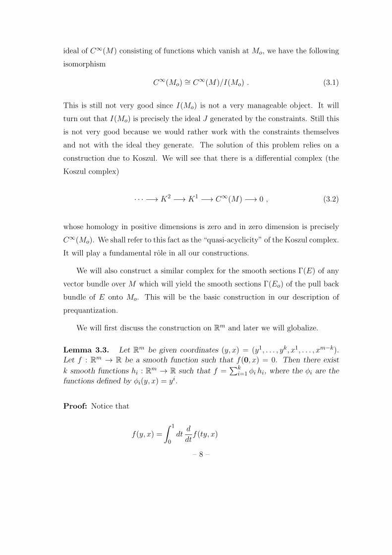
ideal of C∞(M) consisting of functions which vanish at Mo, we have the following

isomorphism

C∞(Mo) ∼= C∞(M)/I(Mo) . (3.1)

This is still not very good since I(Mo) is not a very manageable object. It will

turn out that I(Mo) is precisely the ideal J generated by the constraints. Still this

is not very good because we would rather work with the constraints themselves

and not with the ideal they generate. The solution of this problem relies on a

construction due to Koszul. We will see that there is a differential complex (the

Koszul complex)

· · · −→ K2 −→ K1 −→ C∞(M) −→ 0 , (3.2)

whose homology in positive dimensions is zero and in zero dimension is precisely

C∞(Mo). We shall refer to this fact as the “quasi-acyclicity” of the Koszul complex.

It will play a fundamental role in all our constructions.

We will also construct a similar complex for the smooth sections Γ(E) of any

vector bundle over M which will yield the smooth sections Γ(Eo) of the pull back

bundle of E onto Mo. This will be the basic construction in our description of

prequantization.

We will first discuss the construction on Rm and later we will globalize.

Lemma 3.3. Let Rm be given coordinates (y, x) = (y1, . . . , yk, x1, . . . , xm−k).Let f : Rm → R be a smooth function such that f(0, x) = 0. Then there exist

k smooth functions hi : Rm → R such that f =∑k

i=1 φi hi, where the φi are the

functions defined by φi(y, x) = yi.

Proof: Notice that

f(y, x) =

∫ 1

0dt

d

dtf(ty, x)

– 8 –

=

∫ 1

0dt

k∑i=1

yi (Di f)(ty, x)

=k∑i=1

yi∫ 1

0dt (Di f)(ty, x)

=k∑i=1

φi(y, x)

∫ 1

0dt (Di f)(ty, x) ,

where Di is the ith partial derivative. Defining

hi(y, x)def=

∫ 1

0dt (Di f)(ty, x) (3.4)

the proof is complete.

Therefore, if we let P ⊂ Rm denote the subspace defined by yi = 0 for all i, the

ideal of C∞(Rm) consisting of functions which vanish on P is precisely the ideal

generated by the functions φi.

Definition 3.5. Let R be a ring1. A sequence (φ1, . . . , φk) of elements of R iscalled regular if for all j = 1, . . . , k, φj is not a zero divisor in R/Ij−1, where Ijis the ideal generated by φ1, . . . , φj and I0 = 0. In other words, if f ∈ R and forany j = 1, . . . , k, φj f ∈ Ij−1 then f ∈ Ij−1 to start out with. In particular, φ1 isnot identically zero.

Proposition 3.6. Let Rm be given coordinates (y, x) = (y1, . . . , yk, x1, . . . , xm−k).Then the sequence (φi) in C∞(Rm) defined by φi(y, x) = yi is regular.

Proof: First of all notice that φ1 is not identically zero. Next suppose that

(φ1, . . . , φj) is regular. Let Pj denote the hyperplane defined by φ1 = · · · = φj = 0.

Then by Lemma 3.3 , C∞(Pj) = C∞(Rm)/Ij . Let [f ]j denote the class of a

f ∈ C∞(Rm) modulo Ij . Then φj+1 gives rise to a function [φj+1]j in C∞(Pj)

1 All rings explicitly considered in this paper will be assumed to be commutative

and with unit.

– 9 –

which, if we think of Pj as coordinatized by (yj+1, . . . , yk, x1, . . . , xm−k), turns out

to be defined by

[φj+1]j (yj+1, . . . , yk, x1, . . . , xm−k) = yj+1 . (3.7)

This is clearly not identically zero and, therefore, the sequence (φ1 . . . , φj+1) is

regular. By induction we are done.

We now come to the definition of the Koszul complex. Let R be a ring and

let Φ = (φ1, . . . , φk) be a sequence of elements of R. We define a complex (in the

sense of homological algebra) K(Φ) as follows: K0(Φ) = R and for p > 0, Kp(Φ) is

defined to be the free R module with basis ei1 ∧ · · · ∧ eip | 0 < i1 < · · · < ip ≤ k.

Define a map δK : Kp(Φ) → Kp−1(Φ) by δKei = φi and extending to all of

K(Φ) as an R-linear antiderivation. That is, δK is identically zero on K0(Φ) and

δK(ei1 ∧ · · · ∧ eip) =

p∑j=1

(−1)j−1φij ei1 ∧ · · · ∧ eij ∧ · · · ∧ eip , (3.8)

where aadorning a symbol denotes its omission. It is trivial to verify that δ2K = 0,

yielding a complex

0 −→ Kk(Φ)δK−→ Kk−1(Φ) −→ · · · −→ K1(Φ) −→ R −→ 0 , (3.9)

called the Koszul complex.

The following theorem is a classical result in homological algebra whose proof

is completely straight-forward and can be found, for example, in [13] .

Theorem 3.10. If (φ1, . . . , φk) is a regular sequence in R then the homology ofthe Koszul complex is given by

Hp(K(Φ)) ∼=

0 for p > 0

R/J for p = 0, (3.11)

where J is the ideal generated by the φi.

– 10 –

Therefore the complex K(Φ) provides an acyclic resolution (known as the

Koszul resolution) for the R-module R/J . Therefore if R = C∞(Rm) and Φ is

the sequence (φ1, . . . , φk) of Proposition 3.6 , the Koszul complex gives an acyclic

resolution of C∞(Rm)/J which by Lemma 3.3 is just C∞(Pk), where Pk is the

subspace defined by φ1 = · · · = φk = 0.

We now globalize this construction. Let M be our original symplectic manifold

and Φ : M → Rk be the function whose components are the constraints, i.e.

Φ(m) = (φ1(m), . . . , φk(m)). We assume that 0 is a regular value of Φ so that

Mo ≡ Φ−1(0) is a closed embedded submanifold of M . Therefore for each point

m ∈ Mo here exists an open set U ∈ M containing m and a chart Ψ : U → Rm

such that Φ has components (φ1, . . . , φk, x1, . . . , xm−k) and such that the image

under Φ of U ∩Mo corresponds exactly to the points (0, . . . , 0︸ ︷︷ ︸k

, x1, . . . , xm−k). Let

U be an open cover for M consisting of sets like these. Of course, there will be

some sets V ∈ U for which V ∩Mo = ∅.

To motivate the following construction let’s understand what is involved in

proving, for example, that the ideal J generated by the constraints coincides with

the ideal I(Mo) of smooth functions which vanish onMo. It is clear that J ⊂ I(Mo).

We want to show the converse. That is, if f is a smooth function vanishing on

Mo then there are smooth functions hi such that f =∑

i hi φi. This is always

true locally. That is, restricted to any set U ∈ U such that U ∩Mo 6= ∅, Lemma

3.3 implies that there will exist functions hiU ∈ C∞(U) such that on U

fU =∑i

φi hiU , (3.12)

where fU denotes the restriction of f to U . If, on the other hand, V ∈ U is

such that V ∩Mo = ∅, then not all of the φi vanish and the statement is also

true. There is a certain ambiguity in the choice of hUi . In fact, if δK denotes

the Koszul differential we notice that (3.12) can be written as fU = δKhU , where

hU =∑

i hiUei is a Koszul 1-cochain on U . Therefore, the ambiguity in hU is

– 11 –

precisely a Koszul 1-cocycle on U , but by Theorem 3.10 , the Koszul complex on U

is quasi-acyclic and hence every 1-cocycle is a 1-coboundary. What we would like

to show is that this ambiguity can be exploited to choose the hU in such a way that

hU = hV on all non-empty overlaps U∩V . This condition is precisely the condition

for hU to be a Cech 0-cocycle. In order to analyze this problem it is useful to make

use of the machinery of Cech cohomology with coefficients in a sheaf. For a review

of the necessary material we refer the reader to [14] ; and, in particular, to their

discussion of the Cech-de Rham complex. Our construction is very close in spirit

to that one: in fact, it should properly be called the Cech-Koszul complex.

Let EM denote the sheaf of germs of smooth functions on M and let K =⊕pKp denote the free sheaf of EM -modules which appears in the Koszul complex:

Kp =∧pV⊗EM , where V is the vector space with basis ei. Let Cp(U ;Kq) denote

the Cech p-cochains with coefficients in the Koszul subsheaf Kq. This becomes a

double complex under the two differentials

δ : Cp(U ;Kq)→ Cp+1(U ;Kq) “Cech”

and

δK : Cp(U ;Kq)→ Cp(U ;Kq−1) “Koszul”

which clearly commute, since they are independent. We can therefore define the

“total” complex CKn =⊕

p−q=nCp(U ;Kq) and the “total” differential D = δ +

(−1)pδK on Cp(U ;Kq). The total differential has total degree one D : CKn →

CKn+1 and moreover obeys D2 = 0. Since the double complex is bounded, i.e.

for each n, CKn is the direct sum of a finite number of Cp(U ;Kq)’s, there are

two spectral sequences converging to the total cohomology. We now proceed to

compute them. In doing so we will find it convenient to depict our computations

– 12 –

graphically. The original double complex is depicted by the following diagram.

C0(U ;K2) C1(U ;K2) C2(U ;K2)

C0(U ;K1) C1(U ;K1) C2(U ;K1)

C0(U ;K0) C1(U ;K0) C2(U ;K0)

Upon taking cohomology with respect to the horizontal differential (i.e. Cech co-

homology) and using the fact that the sheaves Kq are fine, being free modules over

the structure sheaf EM , we get

K2(Φ) 0 0

K1(Φ) 0 0

K0(Φ) 0 0

where Kp(Φ) ∼=∧pV⊗C∞(M) are the spaces in the Koszul complex on M . Taking

vertical cohomology yields the Koszul cohomology

H2(K(Φ)) 0 0

H1(K(Φ)) 0 0

H0(K(Φ)) 0 0

Since the next differential in the spectral sequence necessarily maps across columns

it must be identically zero. The same holds for the other differentials and we see

that the spectral sequence degenerates at the E2 term. In particular the total

– 13 –

cohomology is isomorphic to the Koszul cohomology:

HnD∼= Hn(K(Φ)) . (3.13)

To compute the other spectral sequence we first start by taking vertical cohomology,

i.e. Koszul cohomology. Because of the choice of cover U we can use Theorem

3.10 and Lemma 3.3 to deduce that the vertical cohomology is given by

0 0 0

0 0 0

C0(U ; EM/J ) C1(U ; EM/J ) C2(U ; EM/J )

where EM/J is defined by the exact sheaf sequence

0→ J → EM → EM/J → 0 , (3.14)

where J is the subsheaf of EM consisting of germs of smooth functions belonging

to the ideal generated by the φi. Because of our choice of cover, Lemma 3.3 implies

that J (U) agrees, for all U ∈ U , with those smooth functions vanishing on U ∩Mo,

and hence we have an isomorphism of sheaves EM/J ∼= EMo, where EMo

is the sheaf

of germs of smooth functions on Mo. Next we notice that EMois a fine sheaf and

hence all its Cech cohomology groups vanish except the zeroth one. Thus the E2

term in this spectral sequence is just

0 0 0

0 0 0

C∞(Mo) 0 0

Again we see that the higher differentials are automatically zero and the spectral

sequence collapses. Since both spectral sequences compute the same cohomology

we have the following corollary.

– 14 –

Corollary 3.15. If 0 is a regular value for Φ : M → Rk the Koszul complex K(Φ)

gives an acyclic resolution for C∞(Mo). In other words, the cohomology of the

Koszul complex is given by

Hp(K(Φ)) ∼=

0 for p > 0

C∞(Mo) for p = 0, (3.16)

where Mo ≡ Φ−1(0).

Notice that, in particular, this means that the ideal J generated by the con-

straints is precisely the ideal consisting of functions vanishing on Mo. This is

because C∞(Mo) ∼= C∞(M)/I(Mo) since Mo is a closed embedded submanifold.

On the other hand, Corollary 3.15 implies that C∞(Mo) ∼= C∞(M)/J . Hence the

equality between the two ideals.

It may appear overkill to use the spectral sequence method to arrive at Corol-

lary 3.15 . In fact it is not necessary and the reader is urged to supply a proof using

the “tic-tac-toe” methods in [14] . This way one gains some valuable intuition on

this complex. In particular, one can show that way that the sequence Φ is regular

in C∞(M) and that J = I(Mo) without having to first prove Corollary 3.15 . Lack

of space prevents us from exhibiting both computations and the spectral sequence

computation is decidedly shorter.

Suppose now that we want to do the same for sections of vector bundles rather

than with functions. Suppose that E−→M is a vector bundle on M and that the

Eo−→Mo is the restriction of the bundle to Mo. More formally, Eo is the pullback

bundle i−1E via the natural inclusion i : Mo → M . It turns out that this can be

done at almost no extra cost. For this we have to introduce a generalization of the

Koszul complex.

Let R be a ring and E an R-module. We can then define a complex K(Φ;E)

associated to any sequence (φ1, . . . , φk) by just tensoring the Koszul complex K(Φ)

with E, that is, Kp(Φ;E) = Kp(Φ) ⊗R E and extending δK to δK ⊗ 1. Let

H(K(Φ);E) denote the cohomology of this complex. It is naturally an R-module.

– 15 –

It is easy to show that if E and F are R-modules, then there is an R-module

isomorphism

H(K(Φ);E ⊕ F ) ∼= H(K(Φ);E)⊕H(K(Φ);F ) . (3.17)

Hence, if F =⊕

αR is a free R-module then

H(K(Φ);F ) ∼=⊕α

H(K(Φ)) . (3.18)

In particular if Φ is a regular sequence then the generalized Koszul complex with

coefficients in a free R-module is quasi-acyclic. Now let P be a projective module,

i.e. P is a summand of a free module. Then let N be an R-module such that

P ⊕N = F , F a free R-module. Then

H(K(Φ);F ) ∼= H(K(Φ);P )⊕H(K(Φ);N) , (3.19)

which, along with the quasi-acyclicity of H(K(Φ);F ), implies the quasi-acyclicity

of H(K(Φ);P ). How about H0(K(Φ);P )? By definition

H0(K(Φ);P ) ∼= R/J ⊗R P ∼= P/JP . (3.20)

Therefore we have the following algebraic result

Theorem 3.21. If Φ = (φ1, . . . , φk) is a regular sequence in R, and P is a projec-

tive R-module, then the homology of the Koszul complex with coefficients in P is

given by

Hp(K(Φ);P ) ∼=

0 for p > 0

P/JP for p = 0, (3.22)

where J is the ideal generated by the φi.

– 16 –

The relevance of this construction is that the smooth sections of any vector

bundle over M have the structure of a (finitely generated) projective C∞(M)-

module. More precisely, let Eπ−→M be a complex vector bundle of rank r over M

and let Γ(E) denote the space of smooth sections. It is clear that Γ(E) is a module

over C∞(M) where multiplication is defined pointwise using the linear structure

on each fiber. It is straight-forward to prove that Γ(E) is a free rank r C∞(M)-

module if and only if E is a trivial bundle. It can be shown[15] that M has a finite

cover trivializing E. Since on each set of the cover, E is trivial we see that Γ(E) is

finitely generated: just take as a set of generators the local sections on each cover

multiplied by the appropriate elements of a partition of unity subordinate to the

cover.

It can also be shown[15] that given a vector bundle Eπ−→M there exists another

vector bundle Fρ−→M such that their Whitney sum E ⊕ F is trivial. Therefore

Γ(E⊕F ) ∼= Γ(E)⊕Γ(F ) is a free C∞(M) module and we see that Γ(E) is a direct

summand of a free module. In summary, Γ(E) is a finitely generated projective

C∞(M)-module.

After these remarks Theorem 3.21 and Corollary 3.15 provide an immediate

corollary.

Corollary 3.23. Let 0 be a regular value for Φ : M → Rk and let Eπ−→M be

a smooth vector bundle over M . Then the Koszul complex K(Φ; Γ(E)) gives anacyclic resolution of Γ(E)/JΓ(E).

Our next and final result of this section concerns the object Γ(E)/JΓ(E). Let

i : Mo → M denote the natural inclusion. Then if Eπ−→M is a vector bundle

over M denote by i−1E−→Mo the pull-back bundle via i. It will follow from the

following theorem that Γ(E)/JΓ(E) is isomorphic to Γ(i−1E). But first we need

some remarks of a more general nature.

Let ψ : M →M be a smooth map between differentiable manifolds. It induces

a ring homomorphism

ψ∗ : C∞(M)→ C∞(M) (3.24)

– 17 –

defined by ψ∗ f = f ψ for f ∈ C∞(M). This makes any C∞(M)-module (in

particular C∞(M) itself) into a C∞(M)-module, by restriction of scalars: multi-

plication by C∞(M) is effected by precomposing multiplication by C∞(M) with

ψ∗.

Now let Eπ−→M and E

π−→M be vector bundles of the same rank with the

property that there is a bundle map given by the following commutative diagram

Eϕ−→ Eyπ yπ

Mψ−→ M

(3.25)

(i.e. ϕ is smooth fiber-preserving) with the property that ϕ restricts to a linear

isomorphism on the fibers. Then we may form the following C∞(M)-module

C∞(M)⊗C∞(M) Γ(E) (3.26)

which can be made into a C∞(M)-module by extension of scalars: left multiplica-

tion by C∞(M). Define a map ϕ] : Γ(E)→ Γ(E) by

(ϕ]σ)(m) = (ϕm)−1 [σ(ψ(m))] , (3.27)

for all m ∈ M and σ ∈ Γ(E). Then the following can be easily proven[15]

Theorem 3.28. With the above notation, there exists an isomorphism of C∞(M)

modules

C∞(M)⊗ Γ(E) −→ Γ(E) , (3.29)

defined by f ⊗ σ 7→ f · ϕ] σ and where the tensor product is over C∞(M).

– 18 –

In the case we are interested in we have the following commutative bundle

diagram

i−1Ej−→ Eyπo

yπMo

i−→ M

(3.30)

By Theorem 3.28 , we have that

Γ(i−1E) ∼= C∞(Mo)⊗C∞(M) Γ(E) . (3.31)

But C∞(Mo) ∼= C∞(M)/J , whence

Γ(i−1E) ∼= C∞(M)/J ⊗C∞(M) Γ(E)

∼= Γ(E)/JΓ(E) , (3.32)

where the last isomorphism is standard.

Therefore we conclude this section with the following important corollary.

Corollary 3.33. If 0 is a regular value of Φ : M → Rk. Then the Koszul complex

K(Φ; Γ(E)) gives an acyclic resolution of the module of smooth sections of the

pullback of the bundle Eπ−→M via the natural inclusion i : Φ−1(0)→M .

Proof: This is a direct consequence of Corollary 3.23 and the isomorphism of

(3.32) .

§4 BRST COHOMOLOGY

In this section we complete the construction of the algebraic equivalent of sym-

plectic reduction by first defining a cohomology theory that describes the passage

of Mo to M and then, in keeping with our philosophy of not having to work on

Mo, we extend it to a cohomology theory (BRST) which allows us to work with

M from objects defined on M .

– 19 –

To help fix the ideas we shall first discuss functions. A smooth function on

M pulls back to a smooth function on Mo which is constant on the fibers. Con-

versely, any smooth function on Mo which is constant on the fibers defines a smooth

function on M . Since the fibers are connected (after all they arise as integral sub-

manifolds of a distribution) a function is constant on the fibers if and only if it is

locally constant. Since the hamiltonian vector fields Xi associated to the con-

straints φi form a global basis of the tangent space to the fibers, a function f on

Mo is locally constant on the fibers if and only if Xi f = 0 for all i. In an effort to

build a cohomology theory and in analogy to the de Rham theory, we pick a global

basis ωi for the cotangent space to the fibers such that they are dual to the Xi,i.e. ωi(Xj) = δij . We then define the vertical derivative dV on functions as

dV f =∑i

(Xif)ωi ∀ f ∈ C∞(Mo) . (4.1)

Let ΩV (Mo) denote the exterior algebra generated by the ωi over C∞(Mo). We

will refer to them as vertical forms. We can extend dV to a derivation

dV : ΩpV (Mo)→ Ωp+1

V (Mo) (4.2)

by defining

dV ωi = −1

2

∑j,k

fjki ωj ∧ ωk , (4.3)

where the fijk are the functions appearing in the Lie bracket of the hamiltonian

vector fields associated to the constraints: [Xi , Xj ] =∑

k fijkXk; or, equivalently,

in the Poisson bracket of the constraints themselves: φi , φj =∑

k fijk φk.

Notice that the choice of ωi corresponds to a choice of connection on the

fiber bundle Moπ−→M . Let V denote the subbundle of TMo spanned by the Xi.

It can be characterized either as kerπ∗ or as TM⊥o . A connection is then a choice

of complementary subspace H such that TMo = V ⊕ H. It is clear that a choice

– 20 –

of ωi implies a choice of H since we can define X ∈ H if and only if ωi(X) = 0

for all i. If we let prV denote the projection TMo → V it is then clear that acting

on vertical forms, dV = pr∗V d, where d is the usual exterior derivative on Mo.

It follows therefore that d2V = 0. We call its cohomology the vertical coho-

mology and we denote it as HV (Mo). It turns out that it can be computed[16] in

terms of the de Rham cohomology of the typical fiber in the fibration Moπ−→M .

In particular, from its definition, we already have that

H0V (Mo) ∼= C∞(M) . (4.4)

However this is not the end of the story since we don’t want to have to work

on Mo but on M . The results of the previous section suggest that we use the

Koszul construction. Notice that ΩV (Mo) is isomorphic to∧Rk ⊗C∞(Mo) where

Rk has basis ωi. The Koszul complex gives a resolution for C∞(Mo). Therefore

extending the Koszul differential as the identity on∧Rk we get a resolution for

ΩV (Mo). We find it convenient to think of Rk as V∗, whence the resolution of

ΩV (Mo) is given by

· · · −→∧V∗ ⊗ V⊗ C∞(M)

1⊗δK−→∧V∗ ⊗ C∞(M) −→ 0 . (4.5)

This gives rise to a bigraded complex K =⊕

c,bKc,b, where

Kc,b ≡∧cV∗ ⊗

∧bV⊗ C∞(M) , (4.6)

under the Koszul differential δK : Kc,b → Kc,b−1. The Koszul cohomology of this

bigraded complex is zero for b > 0 by (3.18) , and for b = 0 it is isomorphic

to the vertical forms, where the vertical derivative is defined. To make contact

with the usual notation, elements of∧V∗ (respectively,

∧V) are known as ghosts

(respectively, antighosts).

– 21 –

The purpose of the BRST construction is to lift the vertical derivative to K.

That is, to define a differential δ1 on K which anticommutes with the Koszul

differential, which induces the vertical derivative upon taking Koszul cohomology,

and which obeys δ21 = 0. This would mean that the total differential D = δK + δ1

would obey D2 = 0 acting on K and its cohomology would be isomorphic to the

vertical cohomology. This is possible only in the case of a group action, i.e. when

the linear span of the constraints closes under Poisson bracket. In general this is

not possible and we will be forced to add further δi’s to D to ensure D2 = 0. The

need to include these extra terms was first pointed out by Fradkin and Fradkina

in [17] .

We find it convenient to define δ0 = (−1)cδK on Kb,c. We define δ1 on functions

and ghosts (i.e. ωi) as the vertical derivative1

δ1 f =∑i

(Xif)ωi

=∑i

φi , fωi (4.7)

and

δ1 ωi = −1

2

∑j,k

fjki ωj ∧ ωk . (4.8)

We can then extend it as a derivation to all of∧V∗ ⊗ C∞(M). Notice that it

trivially anticommutes with δ0 since it stabilizes∧V∗ ⊗ C∞(M) where δ0 acts

trivially. We now define it on antighosts (i.e. ei) in such a way that it commutes

with δ0 everywhere. This does not define it uniquely but a convenient choice is

δ1ei =∑j,k

fjik ωj ∧ ek . (4.9)

1 Notice that the vertical derivative is defined on Mo and hence has no unique

extension to M . The choice we make is the simplest and the one that, in the

case of a group action, corresponds to the Lie algebra coboundary operator.

– 22 –

Notice that δ21 6= 0 in general, although it does in the case where the fij

k are

constant. However since it anticommutes with δ0 it does induce a map in δ0 (i.e.

Koszul) cohomology which precisely agrees with the vertical derivative dV , which

does obey d2V = 0. Hence δ2

1 induces the zero map in Koszul cohomology. This

is enough (see algebraic lemma below) to deduce the existence of a derivation

δ2 : Kc,b → Kc+2,b+1 such that δ21 + δ0 , δ2 = 0, where , denotes the anticom-

mutator. This suggests that we define D2 = δ0 + δ1 + δ2. We see that

D22 = δ2

0 ⊕ δ0 , δ1 ⊕ (δ21 + δ0 , δ2)⊕ δ1 , δ2 ⊕ δ2

2 , (4.10)

where we have separated it in terms of different bidegree and arranged them in

increasing c-degree. The first three terms are zero but, in general, the other two

will not vanish. The idea behind the BRST construction is to keep defining higher

δi : Kc,b → Kc+i,b+i−1 such that their partial sums Di = δ0 + · · ·+ δi are nilpotent

up to terms of higher and higher c-degree until eventually D2k = 0. The proof

of this statement will follow by induction from the quasi-acyclicity of the Koszul

complex, but first we need to introduce some notation that will help us organize

the information.

Let us define F pK =⊕

c≥p⊕

bKc,b. Then K = F 0K ⊇ F 1K ⊇ · · · is a

filtration of K. Let DerK denote the derivations (with respect to the ∧ product)

of K. We say that a derivation has bidegree (i, j) if it maps Kc,b → Kc+i,b+j . DerKis naturally bigraded

DerK =⊕i,j

Deri,j K , (4.11)

where Deri,j K consists of derivations of bidegree (i, j). This decomposition makes

DerK into a bigraded Lie superalgebra under the graded commutator:

[ , ] : Deri,j K×Derk,lK→ Deri+k,j+lK . (4.12)

We define F pDerK =⊕

i≥p⊕

j Deri,j K. Then FDerK gives a filtration of DerKassociated to the filtration F K of K.

– 23 –

The remarks immediately following (4.10) imply that D22 ∈ F 3DerK. More-

over, it is trivial to check that [δ0 , D22] ∈ F 4DerK. In fact,

[δ0 , D22] = [D2 , D

22]− [δ1 , D

22]− [δ2 , D

22] (4.13)

where the first term vanishes because of the Jacobi identity and the last two terms

are clearly in F 4DerK. Therefore the part of D22 in F 3DerK/F 4DerK is a δ0-

chain map: that is, [δ0 , δ1 , δ2] = 0. Since it has non-zero b-degree, the quasi-

acyclicity of the Koszul complex implies that it induces the zero map in Koszul

cohomology. By the following algebraic lemma (see below), there exists a derivation

δ3 of bidegree (3, 2) such that δ0 , δ3+ δ1 , δ2 = 0. If we define D3 =∑3

i=0 δi,

this is equivalent to D23 ∈ F 4DerK. But by arguments identical to the ones above

we deduce that [δ0 , D23] ∈ F 5 DerK, and so on. It is not difficult to formalize these

arguments into an induction proof of the following theorem:

Theorem 4.14. We can define a derivation D =∑k

i=0 δi on K, where δi are

derivations of bidegree (i, i− 1), such that D2 = 0.

Finally we come to the proof of the algebraic lemma used above.

Lemma 4.15. Let

· · · −→ K2δ0−→ K1

δ0−→ K0 → 0 (4.16)

denote the Koszul complex where Kb =⊕

cKc,b. Let d : Kb → Kb+i, (i ≥ 0) be aderivation which commutes with δ0 and which induces the zero map on cohomology.Then there exists a derivation K : Kb → Kb+i+1 such that d = δ0 , K.

Proof: Since C∞(M) is an R-algebra it is, in particular, a vector space. Let fαbe a basis for it. Then, since δ0 fα = 0, δ0 d fα = 0. Since d induces the zero map in

cohomology, there exists λα such that d fα = δ0 λα. Define K fα = λα. Similarly,

since δ0 dωi = 0, there exists µi such that dωi = δ0 µ

i. Define K ωi = µi. Since

C∞(M) and the ωi generate K0, we can extend K to all of K0 as a derivation

and, by construction, in such a way that on K0, d = δ0 , K. Now, δ0 d ei = d δ0 ei.

– 24 –

But since δ0 ei ∈ K0, δ0 d ei = δ0K δ0 ei. Therefore δ0 (d ei − K δ0 ei) = 0. Since

d ei ∈ Ki+1 for some i ≥ 0, the quasi-acyclicity of the Koszul complex implies

that there exists ξi such that d ei − K δ0 ei = δ0 ξi. Define K ei = ξi. Therefore,

d ei = δ0 , K ei. We can now extend K as a derivation to all of K. Since d and

δ0 , K are both derivations and they agree on generators, they are equal.

Defining the total complex K =⊕

nKn, where Kn =⊕

c−b=nKc,b, we see that

D : Kn → Kn+1. Its cohomology is therefore graded, that is, HD =⊕

nHnD. D is

known as the BRST operator and its cohomology is the classical BRST cohomology.

The total degree is known as the ghost number. We now compute the classical

BRST cohomology. Notice that since all terms in D have non-negative filtration

degree with respect to F K, there is a spectral sequence associated to this filtration

which converges to the cohomology of D. The E1 term is the cohomology of

the associated graded object GrpK ≡ F pK/F p+1K, with respect to the induced

differential. The induced differential is the part of D of c-degree 0, that is, δ0.

Therefore the E1 term is given by

Ec,b1∼=∧cV∗ ⊗Hb(K(Φ)) . (4.17)

That is, Ec,01∼= Ωc

V (Mo) and Ec,b>01 = 0.

The E2 term is the cohomology of E1 with respect to the induced differential

d1. Tracking down the definitions we see that d1 is induced by δ1 and hence it

is just the vertical derivative dV . Therefore, Ec,02∼= Hc

V (M0) and Ec,b>02 = 0.

Notice, however, that the spectral sequence is degenerate at this term, since the

higher differentials d2, d3, . . . all have b-degree different from zero. Therefore we

have proven the following theorem.

Theorem 4.18. The classical BRST cohomology is given by

HnD∼=

0 for n < 0

HnV (Mo) for n ≥ 0

. (4.19)

In particular, H0D∼= C∞(M).

– 25 –

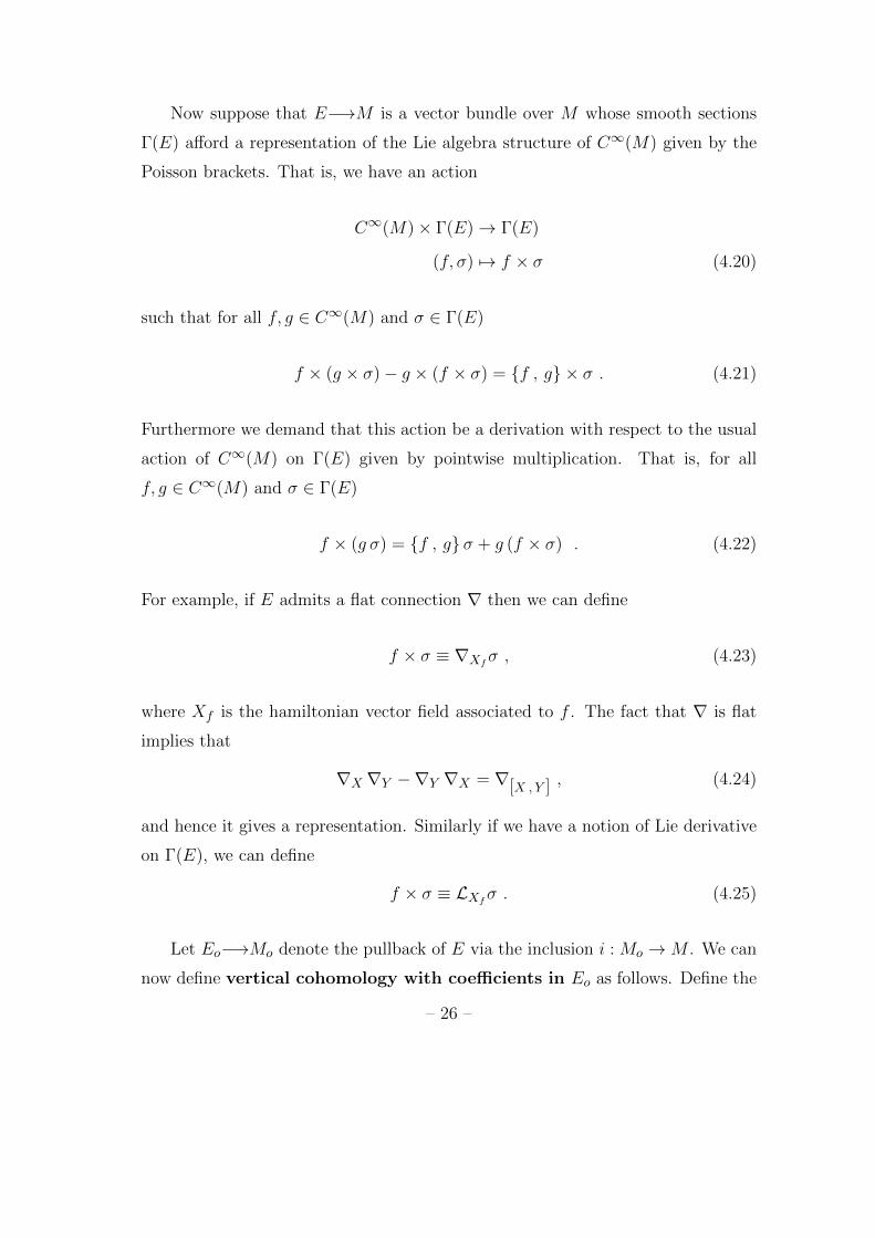
Now suppose that E−→M is a vector bundle over M whose smooth sections

Γ(E) afford a representation of the Lie algebra structure of C∞(M) given by the

Poisson brackets. That is, we have an action

C∞(M)× Γ(E)→ Γ(E)

(f, σ) 7→ f × σ (4.20)

such that for all f, g ∈ C∞(M) and σ ∈ Γ(E)

f × (g × σ)− g × (f × σ) = f , g × σ . (4.21)

Furthermore we demand that this action be a derivation with respect to the usual

action of C∞(M) on Γ(E) given by pointwise multiplication. That is, for all

f, g ∈ C∞(M) and σ ∈ Γ(E)

f × (g σ) = f , gσ + g (f × σ) . (4.22)

For example, if E admits a flat connection ∇ then we can define

f × σ ≡ ∇Xfσ , (4.23)

where Xf is the hamiltonian vector field associated to f . The fact that ∇ is flat

implies that

∇X ∇Y −∇Y ∇X = ∇[X ,Y ] , (4.24)

and hence it gives a representation. Similarly if we have a notion of Lie derivative

on Γ(E), we can define

f × σ ≡ LXfσ . (4.25)

Let Eo−→Mo denote the pullback of E via the inclusion i : Mo →M . We can

now define vertical cohomology with coefficients in Eo as follows. Define the

– 26 –

Eo-valued vertical forms ΩV (Eo) by

ΩV (Eo) ≡ ΩV (Mo)⊗C∞(Mo) Γ(Eo) . (4.26)

We define ∇V by

∇V σ =∑i

(φi × σ)ωi (4.27)

and

∇V ωi = −1

2

∑j,k

fjki ωj ∧ ωk , (4.28)

for all σ ∈ Γ(Eo). We then extend it to all of ΩV (Eo) as a derivation. Just as

for dV , it is easy to verify that ∇2V = 0. We denote its cohomology by HV (Eo).

Moreover notice that for all Eo-valued vertical forms θ

∇V (f θ) = dV f ∧ θ + f ∇V θ . (4.29)

Therefore, H0V (Eo) becomes a C∞(M)-module (under pointwise multiplication)

after the identification of C∞(M) with H0V (Mo). To see this notice that if dV f = 0

and∇V σ = 0, for some σ ∈ Γ(Eo),∇V (f σ) = 0. Moreover, it is easy to verify that

this module is finitely generated and projective. Hence, by general arguments[15],

it is the module of sections of some vector bundle over M .

Now using the Koszul resolution for Γ(Eo) given by Corollary 3.33 we would

like to lift ∇V to a differential D∇ on the complex K(E) =⊕

c,bKc,b(E) where

Kc,b(E) ≡∧cV∗ ⊗

∧bV⊗ Γ(E) . (4.30)

This follows virtually identical steps as for the case of functions. We define

∇0 ≡ (−1)cδK ⊗ 1 on Kc,b(E) . (4.31)

Then, just as before, we define ∇1 by

∇1 σ =∑i

(φi × σ)ωi , (4.32)

– 27 –

∇1 ωi = −1

2

∑j,k

fjki ωj ∧ ωk , (4.33)

and

∇1 ei =∑j,k

fjik ωj ∧ ek . (4.34)

In this way ∇20 = 0 and ∇0 , ∇1 = 0. Therefore filtering K(E) in the

same way as we filtered K and following isomorphic arguments to those leading to

Theorem 4.14 we prove the following theorem.

Theorem 4.35. We can define a derivation D∇ =∑k

i=0∇i on K(E), where ∇iare derivations of bidegree (i, i− 1), such that D2

∇ = 0.

Another spectral sequence argument isomorphic to the one yielding Theorem

4.18 allows us to compute the cohomology of D∇.

Theorem 4.36. The cohomology of D∇ is given by

HnD∇∼=

0 for n < 0

HnV (Eo) for n ≥ 0

. (4.37)

§5 POISSON ALGEBRAS AND POISSON MODULES

So far in the construction of the BRST complex no use has been made of

the Poisson structure of the smooth functions on M . In this section we remedy

the situation. It turns out that the complex K introduced in the last section is a

Poisson superalgebra and the BRST operator D can be made into a Poisson deriva-

tion. Moreover the complex K(E) has a natural Poisson module structure over Kunder which D and D∇ correspond. It will then follow that in cohomology all

constructions based on the Poisson structures will be preserved. This is especially

important in the context of geometric quantization since all objects there can be

– 28 –

defined purely in terms of the Poisson algebra structure of the smooth functions.

In this section we review the concepts associated to Poisson algebras and Poisson

modules. We define the relevant Poisson structures in K and in K(E) and explore

its consequences.

Recall that a Poisson superalgebra is a Z2-graded vector space P = P0⊕P1

together with two bilinear operations preserving the grading:

P × P → P (multiplication)

(a, b) 7→ ab

and

P × P → P (Poisson bracket)

(a, b) 7→ [a , b]

obeying the following properties

(P1) P is an associative supercommutative superalgebra under multiplication:

a(bc) = (ab)c

ab = (−1)|a||b| ba ;

(P2) P is a Lie superalgebra under Poisson bracket:

[a , b] = (−1)|a||b| [b , a]

[a , [b , c]] = [[a , b] , c] + (−1)|a||b| [b , [a , c]] ;

(P3) Poisson bracket is a derivation over multiplication:

[a , bc] = [a , b]c+ (−1)|a||b| b[a , c] ;

for all a, b, c ∈ P and where |a| equals 0 or 1 according to whether a is even or

odd, respectively.

– 29 –

The algebra C∞(M) of smooth functions of a symplectic manifold (M,Ω) is

clearly an example of a Poisson superalgebra where C∞(M)1 = 0. On the other

hand, if V is a finite dimensional vector space and V∗ its dual, then the exterior

algebra∧

(V ⊕ V∗) posseses a Poisson superalgebra structure. The associative

multiplication is given by exterior multiplication (∧) and the Poisson bracket is

defined for u, v ∈ V and α, β ∈ V∗ by

[α , v] = 〈α, v〉 [v , w] = 0 = [α , β] , (5.1)

where 〈, 〉 is the dual pairing between V and V∗. We then extend it to all of∧(V ⊕ V∗) as an odd derivation. Therefore the classical ghosts/antighosts in

BRST possess a Poisson algebra structure. In [7] it is shown that this Poisson

bracket is induced from the supercommutator in the Clifford algebra Cl(V ⊕ V∗)with respect to the non-degenerate inner product on V ⊕ V∗ induced by the dual

pairing.

To show that K is a Poisson superalgebra we need to discuss tensor products.

Given two Poisson superalgebras P and Q, their tensor product P⊗Q can be given

the structure of a Poisson superalgebra as follows. For a, b ∈ P and u, v ∈ Q we

define

(a⊗ u)(b⊗ v) = (−1)|u||b| ab⊗ uv (5.2)

[a⊗ u , b⊗ v] = (−1)|u||b| ([a , b]⊗ uv + ab⊗ [u , v]) . (5.3)

The reader is invited to verify that with these definitions (P1)-(P3) are satisfied.

From this it follows that K = C∞(M)⊗∧

(V⊕V∗) becomes a Poisson superalgebra.

Now let P be a Poisson superalgebra and M = M0 ⊕M1 a Z2-graded vector

space. We will call M a P -module, or a Poisson module over P , if there exist

two bilinear operations preserving the grading

P ×M →M

– 30 –

(a,m) 7→ a ·m

and

P ×M →M

(a,m) 7→ a×m

obeying the following properties

(M1) · makes M a module over the associative structure of P :

a · (b ·m) = (ab) ·m ;

(M2) × makes M into a module over the Lie superalgebra structure of P :

a× (b×m)− (−1)|a||b| b× (a×m) = [a , b]×m ;

(M3) a× (b ·m) = [a , b] ·m+ (−1)|a||b| b · (a×m); where a, b ∈ P and m ∈M .

In particular a Poisson algebra becomes a Poisson module over itself after identify-

ing a ·b with ab and a×b with [a , b]. Notice that equations (4.21) and (4.22) imply

that Γ(E) becomes a Poisson module over C∞(M).

Just like the tensor product of two Poisson superalgebras can be made into

a Poisson superalgebra, if M and N are Poisson modules over P and Q, respec-

tively, their tensor product M ⊗N becomes a P ⊗Q-module under the following

operations:

(a⊗ u) · (m⊗ n) = (−1)|u||m| (a ·m)⊗ (u · n) (5.4)

a⊗ u×m⊗ n = (−1)|u||m| (a×m⊗ u · n+ a ·m⊗ u× n) , (5.5)

for all a ∈ P , u ∈ Q, m ∈ M , and n ∈ N . Again the reader is invited to verify

that with these definitions (M1)-(M3) are satisfied.

– 31 –

Since∧

(V ⊕ V∗) is a Poisson module over itself and Γ(E), for E−→M the

kind of vector bundle discussed in the previous section, is a Poisson module over

C∞(M), their tensor product K(E) becomes a Poisson module over K.

Now let P be a Poisson superalgebra which, in addition, is Z-graded, that

is, P =⊕

n Pn and Pn Pm ⊆ Pm+n and [Pn , Pm] ⊆ Pm+n; and such that the

Z2-grading is the reduction modulo 2 of the Z-grading, that is, P0 =⊕

n P2n and

P1 =⊕

n P2n+1. We call such algebras graded Poisson superalgebras. Notice that

P 0 is an even Poisson subalgebra of P .

For example, letting K = C∞(M)⊗∧

(V⊕V∗) we can define Kn =⊕

c−b=nKc,b.

This way K becomes a Z-graded Poisson superalgebra. Although the bigrading is

preserved by the exterior product, the Poisson bracket does not preserve it. In

fact, the Poisson bracket obeys

[ , ] : Ki,j ×Kk,l → Ki+k,j+l ⊕Ki+k−1,j+l−1 . (5.6)

We can also define the analogous concept of a graded Poisson module over a

graded Poisson superalgebra P in the obvious way: M =⊕

nMn, where M0 =⊕

nM2n and M1 =

⊕nM

2n+1, and both actions of P on M respect the grading.

Therefore K(E) becomes a graded Poisson module over K.

By a Poisson derivation of degree k we will mean a linear map D : Pn → Pn+k

such that

D(ab) = (Da)b+ (−1)k|a| a(Db) (5.7)

D[a , b] = [Da , b] + (−1)k|a| [a , Db] . (5.8)

The map a 7→ [Q , a] for some Q ∈ P k automatically obeys (5.7) and (5.8) . Such

Poisson derivations are called inner. Whenever the degree derivation is inner, any

Poisson derivation of non-zero degree is inner[18] as we now show. The degree

derivation N is defined uniquely by Na = na if and only if a ∈ Pn. In the case

– 32 –

P = K, N is the ghost number operator which is an inner derivation [G , ·], where

G =∑

i ωi ∧ ei, where ei is a basis for V and ωi denotes its canonical dual

basis. Now if a ∈ Pn, and the degree of D is k 6= 0, it follows from (5.8) that

Da =−1

k[DG , a] , (5.9)

and so D is an inner derivation.

If, furthermore, D should obey D2 = 0, and be of degree 1, Q = −DG would

obey [Q , Q] = 0. To see this notice that for all a ∈ Pn

D2a = [Q , [Q , a]] =1

2[[Q , Q] , a] = 0 .

But for a = G we get that [Q , Q] = 0. In this case it is easy to verify that

kerD becomes a Poisson subalgebra of P and imD is a Poisson ideal of kerD.

Therefore the cohomology space HD = kerD/imD naturally inherits the structure

of a Poisson algebra. If let M be a P -module and define the endomorphism D :

M →M by

Dm = Q×m ∀m ∈M , (5.10)

it follows from (M2) and the fact that [Q , Q] = 0 that D2 = 0. Furthermore, using

(M1)-(M3), it follows that its cohomology, HD, inherits the structure of a graded

Poisson module over HD. In particular, H0D is a Poisson module over H0

D.

The BRST operator D constructed in the previous section is a derivation over

the exterior product. Nothing in the way it was defined guarantees that it is a

Poisson derivation and, in fact, it need not be so. However one can show that the

δi’s — which were, by far, not unique — can be defined in such a way that the

resulting D is a Poisson derivation, from which it would immediately follow that

it is inner. It is easier, however, to show the existence of the element Q ∈ K1 such

that D = [Q , ·]. We will show that there exists Q =∑

i≥0Qi, where Qi ∈ Ki+1,i,

such that [Q , Q] = 0 and that the cohomology of the operator [Q , ·] is isomorphic

– 33 –

to that of D. This was first proven by Henneaux in [19] and later in a completely

algebraic way by Stasheff in [4] . Our proof is a simplified version of this latter

proof.

From the discussion previous to Theorem 4.18 we know that the only parts

of D which affect its cohomology are δ0, which is the Koszul differential, and δ1

acting on the Koszul cohomology. Hence we need only make sure that the Qi we

construct realize these differentials. Notice that if Qi ∈ Ki+1,i, [Qi , ·] has terms

of two different bidegrees (i + 1, i) and (i, i − 1). Hence the only term which can

contribute to the Koszul differential is Q0. There is a unique element Q0 ∈ K1,0

such that [Q0 , ei] = δ0 ei = φi. This is given by

Q0 =∑i

ωi φi . (5.11)

Notice that

[Q0 , ei] = δ0 ei = φi (5.12)

[Q0 , ωi] = δ0 ω

i = 0 (5.13)

[Q0 , f ] = (δ0 + δ1) f =∑i

[φi , f ]ωi . (5.14)

There is now a unique Q1 ∈ K2,1 such that [Q1 , ωi] = δ1 ω

i, namely,

Q1 = −1

2

∑i,j,k

fijk ωi ∧ ωj ∧ ek . (5.15)

If we define R1 = Q0 +Q1 we then have that

[R1 , ei] = (δ0 + δ1) ei (5.16)

[R1 , ωi] = (δ0 + δ1)ωi (5.17)

[R1 , f ] = (δ0 + δ1 + δ2) f . (5.18)

In particular, two things are imposed upon us: δ2 f and δ1 ei; the latter imposition

agrees with the choice made in (4.9) .

– 34 –

Letting FK denote the filtration of K defined in the previous section, and

using the notation in which, if O ∈ K is an odd element, O2 stands for 12 [O , O],

the following are satisfied:

R21 ∈ F 3K and [Q0 , R

21] ∈ F 4K . (5.19)

That means that the part of R21 which lives in F 3K/F 4K is a δ0-cocycle, since the

(0,−1) part of Q0 is precisely δ0. By the quasi-acyclicity of the Koszul complex

it is a coboundary, say, −δ0Q2 for some Q2 ∈ K3,2. In other words, there exists

Q2 ∈ K3,2 such that if R2 = Q0 +Q1 +Q2, then R22 ∈ F 4K. If this is the case then

[Q0 , R22] = [R2 , R

22]− [Q1 , R

22]− [Q2 , R

22] . (5.20)

But the first term is zero because of the Jacobi identity and the last two terms are

clearly in F 5K due to the fact that, from (5.6) ,

[F pK , F qK] ⊆ F p+q−1K . (5.21)

Hence, [Q0 , R22] ∈ F 5K, from where we can deduce the existence of Q3 ∈ K4,3

such that R3 = Q0 + Q1 + Q2 + Q3 obeys R23 ∈ F 5K, and so on. It is easy to

formalize this into an induction proof of the following theorem.

Theorem 5.22. There exists Q =∑

iQi, where Qi ∈ Ki+1,i such that [Q , Q] =0.

Now let D = [Q , ·]. Then D2 = 0 and repeating the proof of Theorem 4.18 we

obtain the following.

Theorem 5.23. The cohomology of D is given by

HnD∼=

0 for n < 0

HnV (Mo) for n ≥ 0

. (5.24)

In particular, H0D∼= C∞(M).

– 35 –

From now on we will take D = [Q , ·] to be the classical BRST operator.

Now we consider an arbitrary vector bundle E−→M , whose smooth sections

Γ(E) form a Poisson module over C∞(M). Then we can define D by (5.10) . Then

D decomposes into D =∑

i∇i, where ∇i : Kc,b → Kc+i,b+i−1. We can recover

the ∇i from the Qi by picking the contribution with the right bidegree. Using the

explicit expressions for Q0 and Q1 it is easy to verify that ∇0 and ∇1 defined in

this way agree precisely with the ones in (4.31) , (4.32) , (4.33) , and (4.34) .

This being enough to determine its cohomology, we deduce that the cohomology

of D and that of the operator D∇ of Theorem 4.35 are isomorphic. That is,

Theorem 5.25. The cohomology of D is given by

HnD∼=

0 for n < 0

HnV (Eo) for n ≥ 0

. (5.26)

We conclude, therefore, that the classical BRST construction — both for func-

tions and for sections — is completely compatible with the Poisson structure.

Roughly speaking, the BRST construction feels right at home in the Poisson cat-

egory.

§6 PREQUANTIZATION

Geometric quantization is an attempt to develop a mathematically consistent

and invariant quantization scheme. It tries to overcome the problems of the more

traditional “canonical” quantization. The canonical quantization of finite dimen-

sional systems consists in finding a unitary irreducible representation of the Heisen-

berg algebra

[qa , pb] =√−1h δab , (6.1)

where (q, p) are local coordinates for the phase space of the system we are quantiz-

ing. The Stone–Von Neumann theorem guarantees that there is essentially a unique

– 36 –

such representation2. In this representation — taken, without loss of generality, to

be L2(Rn) — qa is represented by the multiplication operator ψ(q) 7→ qa ψ(q); and

pb is represented by ψ(q) 7→ −√−1hψ′(q). A classical observable f(p, q) is then

represented by f(−√

1h ∂∂q , q).

This has two obvious problems. First, the operator f(−√

1h ∂∂q , q) requires

for its definition that we give an ordering prescription, since q and ∂∂q do not

commute. And second, the Heisenberg algebra is not general coordinate invariant,

so the above prescription depends on the choice of coordinates.

It was Dirac who first noticed the similarity between the algebraic structures

in both quantum and classical mechanics. He observed that the Poisson bracket

seemed to be the classical analogue of the quantum commutator. The fact that

the Poisson bracket has an invariant meaning in the phase space allowed Dirac to

reformulate canonical quantization in an invariant fashion. The Poisson brackets

(i.e. the symplectic structure) thus plays a fundamental role in the Dirac quanti-

zation approach. The Dirac quantization problem consists therefore in finding an

irreducible representation of the Lie algebra (under Poisson bracket) of real smooth

functions as “self-adjoint” operators in a Hilbert space with the properties that the

constant function with value 1 shall be represented by the identity operator and

that, if (q, p) is local chart forming a canonically conjugate pair (i.e. they obey the

Heisenberg algebra), then they shall act irreducibly or at least, in case one wants

to include internal degrees of freedom, with finite reducibility. These conditions

are demanded, for example, by the Heisenberg uncertainty relation.

A celebrated theorem of Van Hove[20] forbids the existence of such a repre-

sentation; although he showed that one could find an irreducible representation of

some subalgebra if one dropped the last condition on canonically conjugate pairs.

2 Strictly speaking, the theorem guarantees the uniqueness up to unitary equiv-

alence of the irreducible representations of the exponentiated (Weyl) form of

the commutation relations.

– 37 –

The geometric quantization program of Kostant[21] and Souriau[22] provides

an invariant method of constructing such representations. The first part of the

method, called prequantization, consists of dropping the irreducibility condition

and constructing a representation of the Lie algebra of smooth functions as “self-

adjoint” operators in a Hilbert space, purely in terms of symplectic data. The

second part of the construction, called polarization, will take care of making

this representation irreducible and in the process restricting the class of functions

which can be quantized. In this section we discuss prequantization. We will review

how prequantum data gets induced under symplectic reduction, and how this is

implemented a la BRST.

Let (M,Ω) be a symplectic manifold. Since dΩ = 0, the symplectic form defines

a class in the real de Rham cohomology group H2dR(M ;R). We say Ω is integral if

this class lies in the image of the map

H2(M ;Z)→ H2(M ;R) ∼= H2dR(M ;R) . (6.2)

If this is the case we speak of an integral symplectic manifold.

If (M,Ω) is an integral symplectic manifold then there exists at least one

complex line bundle E−→M with a hermitian structure, i.e. a sesquilinear map

〈, 〉 : Γ(E)× Γ(E)→ C∞C (M) , (6.3)

which is antilinear in the first factor and linear in the second; and with a connection

∇ : Γ(E)→ Ω1(M)⊗ Γ(E) , (6.4)

such that

(PQ1) 〈, 〉 is parallel with respect to ∇; that is, for all σ, τ ∈ Γ(E),

d〈σ, τ〉 = 〈σ,∇τ〉+ 〈∇σ, τ〉 ;

(PQ2) the symplectic form and the curvature 2-form of the connection are

– 38 –

related by

curv(∇) = −2π√−1Ω .

The triple (E,∇, 〈, 〉) satisfying the above properties will be called prequantum

data for the symplectic manifold (M,Ω). Hence integral symplectic manifolds are

also known as prequantizable symplectic manifolds.

Let dµL denote the Liouville measure on M . This is the measure induced by

the volume form proportional to Ω ∧ · · · ∧ Ω︸ ︷︷ ︸n

for M a 2n-dimensional manifold.

This allows us to define an inner product on Γ(E) by integrating the pointwise

inner product with respect to this measure:

(σ, τ) ≡∫M〈σ, τ〉 dµL . (6.5)

Let ΓL2(E) denote the Hilbert space completion of the subspace of Γ(E) consisting

of sections σ such that ‖σ‖2 ≡ (σ, σ) < ∞. This will become the prequantum

Hilbert space. The prequantization map assigning to a smooth function f an

operator O(f) in ΓL2(E) is the following

f 7→ O(f) ≡ ∇Xf+ 2π

√−1 f , (6.6)

where Xf is the Hamiltonian vector field associated to f , that is, i(Xf ) Ω+df = 0.

The prequantization map obeys the following

O(f)O(g)σ −O(g)O(f)σ = O(f , g)σ , (6.7)

O(f)(gσ) = f , gσ + g O(f)σ , (6.8)

for all σ ∈ Γ(E) and f, g ∈ C∞(M), making Γ(E) into a Poisson module over

C∞(M). Moreover each O(f) is a skew-symmetric operator. That is, if σ, τ ∈

– 39 –

ΓL2(E) are in the domain of O(f) then

(O(f)σ, τ) + (σ,O(f)τ) = 0 . (6.9)

If, in addition, Xf is a complete vector field, O(f) has a skew-self-adjoint extension

and generates, by Stone’s theorem, a one parameter family of unitary operators in

ΓL2(E).

The prequantization map has the property that the only operator of the form

O(f) for some f ∈ C∞(M) which commutes with all the other O(g)’s are the

scalars, corresponding to O(c) for c a constant function on M . Still this repre-

sentation is highly reducible: roughly speaking it consists of integrable functions

of both the momenta and the coordinates. Thus we need to cut down the size of

ΓL2(E). This process, known as polarization, will be the topic of the next sec-

tion. In the rest of this section we show how prequantum data gets induced under

symplectic reduction, and how this works in the BRST context.

In [23] Guillemin and Sternberg proved that in the case of a hamiltonian

group action one could induce prequantum data on the reduced symplectic man-

ifold. Their construction goes roughly as follows. Let Mo denote the constrained

submanifold Φ−1(0), Φ being the moment mapping in their case, and let Eo−→Mo

denote the pull back bundle of E via the inclusion i : Mo → M . They define a

complex line bundle E−→M , where M = Mo/G, by defining its sheaf of sections

to be the g-invariant sections3 of Eo. On Mo, a section σ was g-invariant if and

only if ∇Xσ = 0 for all Killing vectors X. Hence if σ and τ are g-invariant sections,

so is their pointwise inner product 〈σ, τ〉, since

X〈σ, τ〉 = 〈∇Xσ, τ〉+ 〈σ,∇Xτ〉 . (6.10)

A connection ∇ is also constructed by constructing its connection 1-form patchwise.

3 Strictly speaking one must assume that the g action on the sections of Eo

lifts to a G action, to guarantee that the invariant sections correspond to the

sections of some vector bundle over M .

– 40 –

Finally, the inner product was defined integrating the pointwise inner product with

the Liouville measure on M .

We now proceed to see how the prequantum data gets induced a la BRST. We

need not restrict ourselves to the case of a group action. First of all notice that the

sections Γ(E) of the prequantum line bundle form a Poisson module over C∞(M).

Therefore the discussion of the previous sections goes through unaltered. That is,

we construct the graded complex K(E) =⊕

nKn(E) and the derivation

D∇ : Kn(E)→ Kn+1(E) , (6.11)

given by Q× σ, where Q ∈ K1 is the element such that the classical BRST opera-

tor D is given by [Q , ·]. We then define E−→M by defining its space of smooth

sections Γ(E) as H0D∇

. It then becomes a H0D∼= C∞(M) module as shown in

the previous section. Since the prequantization map is precisely one of the maps

incorporated in the Poisson module structure of Γ(E) we have induced all the pre-

quantum data except for the inner product. We will be able to induce a pointwise

inner product but not an inner product. We will comment on the reasons why

later on.

In order to induce a pointwise inner product on H0D∇

it will be first of all neces-

sary to define a pointwise inner product on K(E). To motivate this construction let

us first understand in Poisson terms the invariance of the pointwise inner product

of two invariant sections. This invariance follows from the following fact. Since 〈, 〉is R-linear in both slots it induces a map

〈, 〉 : Γ(E)⊗ Γ(E)→ C∞C (M) ,

which is a C∞(M)-module homomorphism (a homomorphism of Poisson modules

over C∞(M)). That is, if σ, τ ∈ Γ(E) and f ∈ C∞(M) then

[f , 〈σ, τ〉] = 〈f × σ, τ〉+ 〈σ, f × τ〉 . (6.12)

– 41 –

We would now like to extend 〈, 〉 to a K-module homomorphism

〈〈, 〉〉 : K(E)⊗K(E)→ KC . (6.13)

This boils down to essentially defining a linear map

〈, 〉 :∧

(V⊕ V∗)⊗∧

(V⊕ V∗)→∧

(V⊕ V∗) , (6.14)

satisfying, for all φ, ω, θ ∈∧

(V⊕ V∗), the following relations

〈φ ∧ ω, θ〉 = φ ∧ 〈ω, θ〉 = (−1)|φ||ω|〈ω, φ ∧ θ〉 , (6.15)

and

[φ , 〈ω, θ〉] = 〈[φ , ω], θ〉+ (−1)|φ||ω|〈ω, [φ , θ]〉 . (6.16)

There is one obvious candidate:

〈ω, θ〉 = ω ∧ θ . (6.17)

However, although this pointwise inner product will turn out to play an important

role when we discuss duality, it does not seem to be the natural pointwise inner

product on Γ(E). There are other variants of this inner product, differing from it in

a degree dependent sign, which eliminate some of the ±’s which will appear when

we discuss duality. However these signs are not very relevant and for simplicity we

will stick with this pointwise inner product.

At any rate, with this choice we have constructed a sesquilinear map

〈〈, 〉〉 : K(E)×K(E)→ KC , (6.18)

which is invariant under the action of K. It is then clear that, if Z(E) and B(E)

stand for the D∇ cocycles and coboundaries respectively and Z and B stand for

– 42 –

the D cocycles and coboundaries respectively, the mapping 〈〈, 〉〉 obeys

Z(E)× Z(E)→ Z , (6.19)

Z(E)×B(E)→ B , (6.20)

B(E)× Z(E)→ Z ; (6.21)

from where it follows that it induces a well defined map in cohomology. In partic-

ular, since it is graded, it induces a map

〈, 〉 : H0D∇×H0

D∇→ H0

D ⊗ C , (6.22)

which, under the relevant identifications, becomes a pointwise inner product

〈, 〉 : Γ(E)× Γ(E)→ C∞C (M) . (6.23)

This is the best that can be done about the inner product under the present

circumstances. There is no inner product on K(E) which induces, by evaluating it

on D∇ cocycles, the prequantum inner product on M . The reason is the following.

The inner product consists of integrating the pointwise inner product with respect

to the Liouville measure. It is impossible that one can evaluate the inner product of

sections of the prequantum bundle on M by merely picking representative sections

on M and evaluating the inner product there. The reason being that functions on

M are represented by functions on M whose restriction to Mo are constant on the

leaves of the null foliation. But Mo has Liouville measure zero in M and hence

two functions which agree on Mo but which disagree at will away from Mo have

different integrals. Therefore the inner product would not be independent of the

representatives. By tensoring the sections of the prequantum line bundle with half-

forms (see [6] ) the BRST cohomology of this new complex yields objects whose

pointwise inner product can be integrated on M but, again, the integral does not

lift to M .

– 43 –

§7 POLARIZATION

In this section we discuss the second step in the geometric quantization pro-

gram. As we remarked in the previous section, the representation constructed via

prequantization is highly reducible and we must cut down its size. To help fix the

ideas, let us discuss the familiar example of M a cotangent bundle, say T ∗N . In

this case the symplectic form is exact and hence the prequantum line bundle is

trivial. We can therefore choose a global non-vanishing section and hence identify

the space of sections with the complex valued functions themselves. However this

space is far too big: it contains functions of both position and momentum. We

would like to end up with functions of just position. It is then clear what we must

do. We must pick the subspace of the functions which are independent of the

momentum, i.e. they are constant on the fibers of the bundle T ∗Nπ−→N . In other

words, they are the functions which are annihilated by the vector fields tangent

to the fibers. These vector fields span an integrable distribution of TT ∗N , being

exactly the kernel of the derivative of the projection π∗ : TT ∗N → TN . Moreover

this distribution is lagrangian, since locally it is spanned by ∂∂pa in a basis where

the symplectic form is∑

a dqa∧dpa. This distribution, kerπ∗, is the canonical real

polarization (see later) of T ∗N . A general polarization will consist of a suitable

generalization of this object. Of course, in general, a symplectic manifold need not

have a canonical polarization. In this sense, cotangent bundles are special.

We begin then by defining polarizations. By a polarization of a symplectic

manifold (M,Ω) we will mean an involutive lagrangian complex subbundle of the

complexified tangent bundle of M . In other words, let F = m 7→ Fm ⊂ TCmM be

a smooth involutive distribution such that Fm is a complex lagrangian subspace of

TCmM

∼= C⊗RTmM , made into a complex symplectic vector space by extending the

symplectic form C-linearly to a new symplectic form ΩC. Then F is a polarization

of the symplectic manifold (M,Ω) and (M,Ω, F ) is called a polarized symplectic

manifold.

Notice that if F is a polarization, so is F . A polarization is real if F = F . This

– 44 –

is the case if and only if[24] F = C ⊗ V for some involutive lagrangian subbundle

V of TM . The canonical polarization of a cotangent bundle gives rise, upon

complexification, to a real polarization. On the other extreme, a polarization is

totally complex if F ∩F = 0. In this case, TCM ∼= F ⊕F . Therefore F ∩TM =

F ∩√−1TM = 0 and hence F is the graph of a bundle isomorphism TM →

√−1TM . That is, Fm = X +

√−1JmX | X ∈ TmM for some isomorphism

Jm : TmM → TmM . Since Fm is a complex linear subspace we deduce that

J2 = −1 and so it is a complex structure. Moreover since F is lagrangian, for all

X, Y ∈ TM , we have

0 = ΩC(X +√−1JX, Y +

√−1JY )

= Ω(X, Y )− Ω(JX, JY ) +√−1 (Ω(X, JY ) + Ω(JX, Y )) . (7.1)

From the real part of this equation we deduce that J is a symplectomorphism

and from the imaginary part that g(X, Y ) ≡ Ω(X, JY ) is symmetric. Moreover it

follows that J is orthogonal with respect to g. In fact, for all X, Y ∈ TM

g(JX, JY ) = Ω(JX, J2Y )

= Ω(Y, JX)

= g(Y,X)

= g(X, Y ) .

Also, for all X, Y ∈ TM ,

[X+√−1JX , Y +

√−1JY ] = [X , Y ]− [JX , JY ]+

√−1 ([X , JY ] + [JX , Y ]) ,

(7.2)

which, since F is involutive, implies that

J [X , Y ]− J [JX , JY ] = [X , JY ] + [JX , Y ] . (7.3)

In other words, the Nijenhuis tensor vanishes and, by the Newlander-Nirenberg

theorem, (M,J) is a complex manifold whose holomorphic vector fields correspond

– 45 –

to the sections Γ(F ) of F . Therefore, (M,Ω, F ) becomes a pseudo-Kahler manifold,

becoming Kahler only when g is positive definite. In this latter case we say F is a

positive definite polarization.

Let (M,Ω, F ) be a polarized symplectic manifold. Let us define AF to be the

following class of functions

AF = f ∈ C∞C (M) | Xf = 0 , ∀X ∈ Γ(F ) . (7.4)

Alternatively we can characterize these functions as follows.

Proposition 7.5. AF consists precisely of those functions in C∞C (M) whose as-

sociated hamiltonian vector fields are in Γ(F ).

Proof: By definition, a function f ∈ C∞C (M) belongs to AF if and only if Xf = 0

for all X ∈ Γ(F ). But Xf = df(X) = ΩC(X,Xf ). Hence f ∈ AF if and only if

Xf ∈ Γ(F⊥

). But F is lagrangian, so that F⊥

= F . Thus f ∈ AF if and only if

Xf ∈ Γ(F ).

Corollary 7.6. AF is an abelian Poisson subalgebra of C∞C (M).

Proof: If f, g ∈ AF then for all X ∈ Γ(F ), Xf = Xg = 0. Therefore X(fg) =

(Xf)g + f(Xg) = 0, so fg ∈ AF . Moreover, f , g = ΩC(Xf , Xg) which is zero

by the previous Proposition and the fact that F is lagrangian.

In some cases, e.g. F a totally complex polarization, AF is a maximal abelian

subalgebra of C∞C (M). This, in fact, is sometimes taken to be the algebraic defi-

nition of a polarization of a Poisson algebra[25]. Let us now define another class of

functions

NF = f ∈ C∞C (M) | [Xf , Y ] ∈ Γ(F ) , ∀Y ∈ Γ(F ) . (7.7)

That is, NF consist of those functions whose hamiltonian vector fields lie in the

normalizer of Γ(F ). Hence by general properties of normalizers NF is a Lie subal-

gebra of C∞C (M) and that AF ⊂ NF is an abelian ideal. However, in general, NF

is not a Poisson subalgebra of C∞C (M).

– 46 –

Now let Γ(E) denote the smooth sections of the prequantum line bundle on

M. We now define the polarized sections

ΓF (E) = σ ∈ Γ(E) | ∇Xσ = 0 , ∀X ∈ Γ(F ) . (7.8)

If F is a totally complex polarization then E is a holomorphic line bundle and

we can choose ∇ to be a holomorphic connection. In this case, ΓF (E) correspond

to the holomorphic sections. We leave it as an exercise to verify that ΓF (E) is a

Poisson module over AF and a Lie submodule over NF . In fact, NF is the maximal

Lie subalgebra of C∞C (M) stabilizing ΓF (E).

The quantum Hilbert space in the geometric quantization program is precisely

the Hilbert space completion of the polarized sections of finite norm. For general

polarizations there may not be any polarized sections of finite norm. Indeed, sup-

pose that P is not totally complex. Then the norm of a polarized section is invariant

on the leaves of the foliation defined by the integrable distribution D = P ∩ P . If

these leaves are non-compact then there may not be any sections of finite norm.

This obstacle can be overcome via “half-form” quantization, which naturally yields

objects which can be integrated in the space of leaves M/D. Half-form quantization

consists in tensoring the pre-quantum line bundle with the bundle of half-forms in

such a way that the point-wise inner product does not just yield a function to be

integrated with respect to the Liouville form, but actually yields a form which can

be integrated in the appropriate space. We will not discuss half-form quantization

in this paper, except to note that our algebraic constructions extend naturally to

this case since the module of smooth sections of the new pre-quantum bundle is

also a Poisson module. Supposing that the polarization is totally complex but not

positive definite we may still find that there are no polarized sections of finite norm.

In fact, let za be a local holomorphic chart which trivializes the pre-quantum

line bundle and relative to which the symplectic form is

Ω =i

2gabdz

a ∧ dzb . (7.9)

The inner product, after identifying holomorphic sections with holomorphic func-

– 47 –

tions, is just the usual L2 inner product of holomorphic functions on an open set of

Cn with measure e−12gabz

azbdzdz. If gab is not positive definite, i.e. if the polariza-

tion is not positive definite, the exponential grows in the negative directions and,

if the image of the chart is unbounded in those directions, there will be no holo-

morphic integrable functions. Based on this considerations we will often restrict

ourselves to positive definite (totally complex) polarizations.

Having defined the Hilbert space as the space of polarized integrable sections,

we notice that the only readily quantizable observables are the (real) functions in

NF . In order to quantize other observables one must resort to ways of pairing

Hilbert spaces obtained from different polarizations. We will not discuss this topic

here but rather refer the interested reader to any of the standard references on

geometric quantization[6].

Now suppose that (M,Ω) admits a hamiltonian action of a connected Lie group

G. A polarization F is G-invariant if the induced action of G on TCM preserves

F . Since G is connected, F is G-invariant if and only if for all Killing vectors X,

[X , Y ] ∈ Γ(F ) ∀Y ∈ Γ(F ) . (7.10)

In particular, this implies that

φX , f ∈ AF ∀ f ∈ AF , (7.11)

from where it follows that AF is a g-submodule of C∞C (M).

In [23] Guillemin and Sternberg showed that a positive definite G-invariant

polarization on (M,Ω) induces canonically a positive definite polarization F on

the reduced manifold (M, Ω). Let Fo be the subbundle of TCMo given by Fo =

F ∩ TCMo. The by G-invariance, Fo induces an involutive lagrangian subbundle

of TCM . Since F is G-invariant, the φX belong to NF and hence the polarized

sections become a g-module. The polarized sections ΓF

(M) are precisely the g-

invariant polarized sections on Mo, that is, ΓFo(Mo)

g.

– 48 –

In [7] Kostant and Sternberg discussed BRST quantization for the case of a

group action in the spirit that quantizing the “ghost” part (∧

(g∗ ⊕ g)) and the

“matter” part (C∞(M)) could be done independently. The quantization of∧

(g∗⊕g) relied on the observation that the Clifford algebra Cl(g⊕g∗) is naturally filtered

and the associated graded object to this filtration is precisely∧

(g∗ ⊕ g). That is,

we have a canonical isomorphism of vector spaces c : Cl(g∗⊕g)→∧

(g∗⊕g), which

is to be thought of as “classical limit”. For finite dimensional g, Cl(g∗⊕ g) has, up

to isomorphism, a unique irreducible module S and thus it can be identified with

EndS. A quantization of∧

(g∗ ⊕ g) was defined in [7] to be a map∧

(g∗ ⊕ g) →EndS induced from a map q :

∧(g∗⊕ g)→ Cl(g∗⊕ g) which is an inverse of c. No

natural inverse exists and the choice of q corresponds to an ordering prescription.

A model for S can be constructed by choosing a maximal isotropic subspace

of g⊕ g∗, that is, a subspace N ⊂ g⊕ g∗ such that N⊥ = N , for ⊥ the orthogonal

complement with respect to the inner product on g ⊕ g∗ induced by the dual

pairing. For example one could take N to be g or g∗. Having chosen a maximal

isotropic subspace N , let P be a complementary maximal isotropic subspace, i.e.

g⊕ g∗ = N ⊕ P . Then a model for S is given by

S ∼=∧

(g∗ ⊕ g)/I(N) ∼=∧P , (7.12)

where I(N) is the ideal generated by N .

The crucial observation is that∧P is a maximal abelian subalgebra (under

Poisson bracket) of∧

(g∗⊕g) and, in analogy with the case of a symplectic manifold,

can be considered to be the polarized functions and, in this case, the polarized

sections. Hence a choice of maximal isotropic subspace N is equivalent to a choice

of polarization.

We will see that in many cases, e.g. the case of a totally complex polarization,

a particular polarization is imposed on∧

(g∗ ⊕ g). In this context, therefore, the

quantization of the “matter” and the “ghosts” part go hand in hand.

– 49 –

In analogy with the group case, we define a polarization F in the symplectic

manifold (M,Ω) to be invariant with respect to a set of first class constraints

φi if and only if φi ∈ NF for all i. In other words, if [Xi , Y ] ∈ Γ(F ) for all

Y ∈ Γ(F ). Let F be an invariant polarization. We then consider the subspace of

K(E) consisting of polarized sections:

∧(V∗ ⊕ V)⊗ ΓF (E) . (7.13)

We would like to consider the prequantum BRST operator D∇ acting on this

subspace and define the physical Hilbert space as its cohomology (at least for ghost

number zero). However the BRST operator may not leave this subspace invariant.

For example, let ek ⊗ σ be an element in V⊗ ΓF (E). Then

D∇(ek ⊗ σ) =∑i

Qi × (ek ⊗ σ) . (7.14)

If this is to belong to∧

(V∗⊕V)⊗ΓF (E) each piece with a different bidegree must

belong to∧

(V∗ ⊕ V) ⊗ ΓF (E). In particular the (0, 0) piece must be a polarized

section. The (0, 0) piece is just φk σ, which is a polarized section if and only if

φk ∈ AF .

If the polarization is totally complex AF corresponds to holomorphic functions.

Since φk is a real non-constant function it cannot be holomorphic. Hence φk σ is not

a polarized section and the BRST operator does not stabilize∧

(V∗⊕V)⊗ΓF (E).

If we divide out by the ideal generated by V then this term is not present. So we

are forced to polarize the ghosts in such a way that only∧V∗ appears. We thus

define the complex KF (E) by

KF (E) =∧V∗ ⊗ ΓF (E) . (7.15)

It is then clear that the only part of D∇ which survives is ∇1 since it has b-degree

zero. It clearly obeys ∇21 = 0, since it was only V which gave us a hard time at

that.

– 50 –

The quantum BRST cohomology — for the case of a totally complex polariza-

tion — is therefore the cohomology of the complex

· · · −→∧cV∗ ⊗ ΓF (E)

∇1−→∧c+1V∗ ⊗ ΓF (E) −→ · · · . (7.16)

In the case of a group action ∇1 agrees with the Lie algebra coboundary operator

and hence the quantum BRST cohomology is precisely the Lie algebra cohomology

with coefficients in the module of polarized sections: H(g; ΓF (E)).

There in one striking fact about this result. No part of the quantum BRST

operator carries the information concerning the restriction to Mo; since, in fact,

the only part with this information was the Koszul differential ∇0. A heuristic

explanation can be given as follows. In the case of a totally complex polarization,

ΓF (E) are holomorphic sections. By the uniqueness of analytic continuation, a

holomorphic section on M in completely determined once you know it on a real

submanifold Mo; in other words, there is a unique extension to a holomorphic

section on M .

Another instance when a polarization is imposed on the ghost part is in the

case a semisimple group action and F is a polarization for which AF is a maximal

abelian subalgebra of C∞C (M). Let h denote the subalgebra of g defined by

X ∈ h⇔ φX ∈ AF . (7.17)

Notice that h is an abelian subalgebra of g since the map X 7→ φX is a Lie algebra

morphism and AF is abelian. But moreover h is an ideal. To see this notice that

if X ∈ h, Y ∈ g then for all f ∈ AF

φ[X ,Y ] , f = φX , φY , f

= φX , φY , f+ φX , f , φY . (7.18)

Since F is invariant φY , f ∈ AF and both terms are Poisson brackets of elements

in AF and because AF is abelian they vanish. Since φ[X ,Y ] commutes with AF , it

– 51 –

must, by maximality, be in AF itself. Therefore [X , Y ] ∈ h and hence it is an ideal.

If g is semisimple it cannot have any abelian ideals and thus h is zero. Therefore

no φX belongs to AF and, once again, D∇ does not stabilize∧

(g∗ ⊕ g) ⊗ ΓF (E)

unless we polarize the ghost part in such a way that only∧g∗ ⊗ ΓF (E) is left.

In the case of a general polarization it is not clear that a specific polarization

of the ghost part is forced, but in any case we may always choose to polarize

the ghosts in such a way that the resulting quantum BRST complex is (7.16) .

With this choice of polarization the explicit form of the ∇i for i 6= 1 is irrelevant.

This makes the quantization much simpler than what one might have originally

expected. Therefore we choose to work with this polarization for the remainder of

this section.

We end this section with a brief comment about the inner product. We re-

marked in the previous section how it seems impossible to calculate the inner

product on M by evaluating the inner product on M on suitable representatives,

due to the geometric nature of the inner product. It may seem, at least with the

chosen polarization, that this problem could be obviated since holomorphic sections

are uniquely characterized by their behavior on Mo. Still, if the gauge orbits are

not compact the integrable polarized sections on M and M may not correspond.

Of course, one choose a quantization prescription in which one always compute

everything on M , but it is then not clear how to show that this quantum theory

agrees with the theory in M .

There are other problems surrounding the inner product. Ideally, in the purest

BRST philosophy, we would like to be able to compute everything pertaining to

objects in M by choosing representative objects in M (cocycles of the relevant

BRST cohomology) and computing with them in M . This requires certain com-

patibility conditions, namely that the cohomology inherits the relevant structure

from the cochains. In the case of the polarized sections, we would like the inner

product to be induced and we see that this does not occur in general, because

of the problem with the integration. But even without the integral, we have the

– 52 –

problem of defining a reasonable pointwise inner product. In the last section we

gave one which descends to a pointwise inner product in cohomology, but it has a

major drawback. The norm of the polarized sections (elements in the zeroth BRST

cohomology) is always zero, since the inner product pairs cocycles of complemen-

tary ghost number. We have not been able to find a pointwise inner product which

descends to cohomology and which is non-zero when restricted to just cocycles of

zero ghost number.

§8 DUALITY IN QUANTUM BRST COHOMOLOGY

Duality theorems in BRST cohomology have recently attracted some attention.

In [8] we proved a duality theorem for the quantum BRST cohomology in the

context of a Fock space representation with a mild finiteness hypothesis. The

results did not depend on the Fock space context but we did assume the existence

of a non-degenerate inner product on the space of states with respect to which

the BRST operator was (anti-)hermitian. This assumption, we believed, was well

founded on physical grounds. From this duality we then proved also a duality

on operators. In [9] Marc Henneaux obtained similar duality theorems but with

weaker assumptions. In particular he dispensed with the notion of an inner product

to prove the operator duality. He only needs an non-degenerate inner product

in order to turn this around and obtain a duality for the states. The finiteness

assumption, however, is still key in his proofs.

For the classical BRST cohomology and in the case of compact orientable

gauge orbits, a duality theorem was proven in [16] which is a manifestation of the

Poincare duality on the fibers. This result had been conjectured already in [9] at

least for the case of a trivial bundle Mo−→M .

There is a peculiar difference between the classical and quantum versions of

the duality in BRST cohomology. In the quantum case there are states with both

negative and positive ghost numbers and the duality is a symmetry between the

– 53 –

cohomologies at +n and −n ghost numbers:

Hnquantum

∼= H−nquantum ; (8.1)

whereas in the classical case — due to the vanishing of BRST cohomology for

negative ghost number — the duality is a symmetry between complementary di-

mensions

Hnclassical

∼= Hk−nclassical . (8.2)

We also saw in the last section how the quantum BRST cohomology (at least for

our choice of polarization) had no states of negative ghost number. Hence it seems

at first sight that we will not be able to obtain a duality similar to that in (8.1) .

The resolution of this apparent paradox is that the classical and quantum ghost

numbers don’t quite correspond. We will see that for the ghost number operator

to be antihermitian — a fact assumed in [8] — we must shift the ghost number

by −k2 , i.e. we must normal order. In this case and assuming that the polarization

is positive definite (notice that this already implies that it is totally complex) and

modulo some conditions on the constraints we will recover an isomorphism a la

(8.1) . However shifting the ghost number operator by a constant affects the ghost

number of the states but not the one of the operators. In particular there will

be operators which are BRST invariant and which have negative ghost number.

These do not come from quantizing BRST invariant observables, since classical

BRST cohomology is zero for negative ghost number. In fact, as remarked in [9] ,

they seem to come from distributions rather than from smooth functions.

From now on we assume that the polarization is positive definite. As remarked

in the last section this forces a polarization on the ghost part in such a way that

only the ∇1 part of the BRST operator remains. The idea behind the proof of

the duality is very simple and it is similar in spirit to that in [8] . We will define

a positive definite inner product on the complex KF (E). This will allow us to

define a formal adjoint of the BRST operator and a BRST laplacian. Then we will

– 54 –

prove a Hodge decomposition for the BRST complex and from this the duality will

follow.

We now define the inner product. The inner product splits as a product of two

inner products: the one on the “matter” part and the one on the “ghost” part. We

will choose the one on the matter part to be the prequantum inner product: the

integral of the pointwise inner product with respect to the Liouville measure. For

the ghost part we will take the following. Fix a non-zero “volume” form ε ∈∧kV∗.

Since∧kV∗ is one dimensional any other k-form is proportional to ε. We define

the Berezin integral on∧V∗ by

∫Ber

ω = 0 , ∀ω ∈∧p 6=kV∗ (8.3)

∫Ber

λε = λ , ∀λ ∈ R . (8.4)

We then define the inner product of forms by

〈ω, θ〉 = (−i)p(k−p)∫

Ber

ω ∧ θ , (8.5)

for ω ∈∧pV∗ and i =

√−1. The reason for the factors of i is the hermiticity of

the inner product on KF (E):

(ω ⊗ σ, θ ⊗ τ) = (−i)p(k−p)∫M〈σ, τ〉 dµL ·

∫Ber

ω ∧ θ , (8.6)

for ω ∈∧pV∗. Notice that this is zero unless θ ∈

∧k−pV∗. Let us define an element

of KF (E) to be integrable if it belongs to∧V∗⊗ΓF (E)fin, where ΓF (E)fin denotes

the subspace of the polarized sections of finite norm.

In order for the ghost number operator to be skew-adjoint we will have to

redefine it by shifting it by an appropriate constant. The ghost number operator is

– 55 –

given by N =∑k

i=1 ε(ωi)ı(ei), where ε and ı are the exterior and interior product

operations on∧V∗. In particular notice that ı(ei) is a derivation which can be

“integrated by parts” in the Berezin integral. We shift N by a constant c and

notice that, if Nc ≡ N − c, then for all ω ⊗ σ, θ ⊗ τ ∈ KF (E) integrable, it is easy

to show that

(Nc ω ⊗ σ, θ ⊗ τ) = (k − 2c)(ω ⊗ σ, θ ⊗ τ)− (ω ⊗ σ,Nc θ ⊗ τ) ; (8.7)

from where it follows that for c = k2 we obtain a skew-adjoint ghost number oper-

ator.

The BRST operator for this choice of polarization is given by the ∇1 piece:∑i

ε(ωi)O(φi)−1

2

∑i,j,k

fijkε(ωi)ε(ωj)ı(ek) . (8.8)

Let ω ⊗ σ ∈ KpF (E), θ ⊗ τ ∈ KF (E) be integrable. Then after a straight-forward

calculation we find

(∇1 ω ⊗ σ, θ ⊗ τ) = ±

(ω ⊗ σ,∇1 θ ⊗ τ) +∑i,j

(ω ⊗ σ, fijjε(ωi)θ ⊗ τ)

, (8.9)

where the explicit dependence of ± on p, k is of no consequence. We therefore see

that if∑

i,j fijj = 0 for all i, then ∇†1 = ±∇1, and therefore an inner product

is induced in cohomology. To see this notice that the only condition needed for

the inner product to descend to cohomology is that the cobundaries be orthogonal

to the cocycles, that is, ker∇1 ⊆ ker∇†1. For the case of a group action, the

condition∑

i,j fijj = 0 is precisely that tr ad(ei) = 0, that is, that g be unimodular.

This condition is equivalent to the existence of a bi-invariant metric on the group

manifold. The condition that the inner product descends to cohomology is, of

course, very desirable on physical grounds since gauge related states should be

physically equivalent. In this case, however, this inner product is not the physical

inner product, and we make this choice, not on physical grounds, but to be able

to prove duality.

– 56 –

Therefore from now on we assume that for all i,∑

i,j fijj = 0. In this case,

∇†1 = ±∇1 acting on integrable elements of KF (E). We now define a Hodge-type

operator. For definiteness and with no loss in generality, let us fix the following

volume form on∧V∗: ε = ω1∧· · ·∧ωk. We define the operator ? :

∧pV∗ →∧k−pV∗

as follows:

?(1) = ε ; (8.10)

?(ε) = 1 ; (8.11)

?(ωi1 ∧ · · · ∧ ωip) = ±ωip+1 ∧ · · · ∧ ωik ; (8.12)

where (i1, . . . , ik) is a permutation of (1, . . . , k) and ± refers to the sign of the

permutation. It is trivially verified that ?2 = (−1)p(k−p) on∧pV∗. Let us then

define ? = (i)p(k−p)? on∧pV∗. It clearly satisfies ?2 = 1. This allows to redefine

the inner product (, ) in such a way that it is now positive definite. In fact, let’s

define a new inner product

(Ψ,Ξ)? ≡ (Ψ, ?Ξ) , (8.13)

for Ψ,Ξ ∈ KF (E). If ω ⊗ σ, θ ⊗ τ ∈ KF (E) the new inner product becomes

(ω ⊗ σ, θ ⊗ τ)? =

∫M〈σ, τ〉 dµL ·

∫Ber

ω ∧ ? θ . (8.14)

It follows that this inner product is positive definite. To see this notice that

the inner product on the sections is positive definite by construction. And to show

that the other part is positive definite, we need only exhibit an orthonormal basis.

Let I = (i1, . . . , ip) denote a sequence 1 ≤ i1 < · · · < in ≤ k. Then if we define

ωI = ωi1 ∧ · · · ∧ωip , the collection of all such ωI forms a basis for∧V∗. On this

basis, it is easy to see that∫Ber

ωI ∧ ? ωJ = δIJ =

1 for I = J

0 otherwise. (8.15)

Moreover we see that the integrable elements of KF (E) are precisely those elements

– 57 –

of KF (E) which have finite norm with respect to this new inner product. We let

ΓF,L2(E) denote the Hilbert space completion of this space with respect to this

new inner product.

The BRST operator ∇1 is generally unbounded so we have to be careful and

specify its domain. From the definition of ΓF,L2(E), it is clear that the BRST

operator is densely defined, since it is defined on the integrable elements and the

ΓF,L2(E) is their closure.4 Now let ∇∗1 denote the adjoint of ∇1 with respect to

the new inner product. Notice that on∧V∗ ⊗ ΓF (E)fin

∇∗1 = ±?∇1? . (8.16)

In particular, notice that ∇∗1 is also densely defined. Therefore ∇1 is a closeable

operator with minimal closed extension ∇1 ≡ (∇∗1)∗. We can therefore define the

BRST operator to be the closure of ∇1. To avoid cumbersome notation we will

denote this also by ∇1.

Since ∇∗1 is closed, ker∇∗1 is a closed subspace of ΓF,L2(E) and hence we have

the following orthogonal decomposition

ΓF,L2(E) = ker∇∗1 ⊕ (ker∇∗1)⊥ . (8.17)

Now, since ∇1 is closed, (ker∇∗1)⊥ is precisely the closure of im∇1. Thus we have

the following orthogonal decomposition

ΓF,L2(E) = ker∇∗1 ⊕ im∇1 . (8.18)

Therefore we can decompose ker∇1 as an orthogonal direct sum

ker∇1 = ker∇1 ∩ ker∇∗1 ⊕ im∇1 . (8.19)

4 We are assuming here that the constraints are such that the BRST operator

stabilizes ΓF (E)fin. This is always the case, for instance, if M admits a finite

holomorphic atlas.[26]

– 58 –

Therefore we have the following isomorphism

Hquantum BRST ≡ ker∇1/im∇1∼= ker∇1 ∩ ker∇∗1 , (8.20)

where we have defined the BRST cohomology in this way for convenience.5

Moreover this isomorphism is an isomorphism of graded (by ghost number)

vector spaces. Because of (8.16) , ? stabilizes ker∇1 ∩ ker∇∗1. Since it connects

opposite ghost numbers and ?2 = 1, it is an isomorphism between the BRST

cohomology spaces at opposite ghost number. Thus we have proven the following

duality theorem.

Theorem 8.21. If the constraints satisfy the condition∑

i,j fijj = 0 for all i,

there is an isomorphism

Hgquantum BRST

∼= H−gquantumBRST . (8.22)

Notice that the problems of closure as well as the condition that the constraints

stabilize the integrable subspace is unnecessary if M is assumed compact, since in

this case the space of holomorphic sections is finite.

§9 CONCLUSIONS AND OPEN PROBLEMS

In this paper we have shown how all of the objects relevant to the geometric

quantization program have an associated BRST cohomology theory describing their

reduction via a symplectic quotient of the original symplectic manifold on which

they are described. Moreover we have seen that the BRST cohomology preserves

all Poisson structures.

5 Since im∇1 is, in general, infinite dimensional it is not necessarily closed.

Factoring out by a non-closed subspace results in the natural surjection not

being continuous and in the factor object not being complete.

– 59 –

The coherence between the BRST construction and the Poisson structures

suggests that we can phrase this construction in purely algebraic terms in the

category of “constrained” Poisson algebras. That is, given a Poisson algebra P

with a distinguished set of elements Φ = φi such that the ideal J they generate

is a Lie subalgebra of P and such that the sequence Φ is regular we can construct

a BRST cohomology theory which reduces P to another Poisson algebra. This is

precisely the point of view taken by Stasheff[4],[5]. We can extend this further by

homologically reducing Poisson modules of P . In the same way we show that a

BRST theory exists which reduces the Poisson module into a Poisson module of

the homological reduction of P . Moreover properties such as finitely generated

and projective are preserved under reduction. We can also define algebraically

a polarization of P as a maximal abelian Poisson subalgebra of P . However we

have not been able to prove that maximal abelian subalgebras correspond under

homological reduction. We have not been able to see how the algebraic analogues

of inner products get induced, although the algebraic analogues of pointwise inner

products can be induced.

The power of the algebraic approach lies in the fact that all the objects in

the geometric quantization program can be defined purely algebraically without

the assumption that the Poisson algebra P or its homological reduction are the

Poisson algebras of symplectic manifolds. This is the case, for example, in Yang-

Mills, where the reduced phase space has singularities[27]. We think that this

particular formulation of BRST quantization can play a fundamental role in the

quantization of such physically relevant systems.

There is another method of quantization which is based purely on the Pois-

son structure of the classical observables: the theory of deformations of Poisson

algebras[28]. It would be interesting to see under what conditions, if any, the

deformations of a Poisson algebra and of its homological reduction correspond.

Finally there are several obvious extensions to these constructions: to the

case of supermanifolds in the sense of Kostant, to arbitrary symplectic Banach

– 60 –

manifolds, and, more importantly, to the case of nonregular constraints[29]. The

extensions to supermanifolds and to the non-regular case should be completely

straight-forward; but the extension to infinite dimensional manifolds may pose

problems having to do with the convergence of the spectral sequences used in

Sections 3 and 4.

ACKNOWLEDGEMENTS

We are grateful to Marc Henneaux for the great benefits we have derived from

our correspondence with him on this and other related topics. We also thank

E. Barrios, Francisco Figueirido, Blaine Lawson, and Eduardo Ramos for conver-

sations. One of us (J.M.F.) thanks Krzysztof Galicki for his hospitality, for the

opportunity to give a talk at Rice University on a part of this paper, and for

making available the Gothic fonts used throughout.

REFERENCES

[1] C. Becchi, A. Rouet, and R. Stora, Phys. Lett. 52B (1974) 344, Comm. Math.

Phys. 42 (1975) 127, and Ann. of Phys. 98 (1976) 287.

[2] I. V. Tyutin, Lebedev Preprint FIAN no. 39 (1975).

[3] I. A. Batalin and G. A. Vilkovisky, Phys. Lett. 69B (1977) 309

M. Henneaux, Phys. Reports 126 (1985) 1

D. McMullan, J. Math. Phys. 28 (1987) 428

A.D. Browning and D. McMullan, J. Math. Phys. 28 (1987) 438

B. Kostant and S. Sternberg, Ann. of Phys. 176 (1987) 49

J. Stasheff, Bull. Am. Math. Soc. 19 (1988) 287

M. Dubois-Violette, Ann. Inst. Fourier 37,4 (1987) 45

M. Henneaux and C. Teitelboim, Comm. Math. Phys. 115 (1988) 213

J. M. Figueroa-O’Farrill and T. Kimura, (Stony Brook Preprint ITP-SB-88-81

(rev.))

[4] J. Stasheff, Bull. Am. Math. Soc. 19 (1988) 287

– 61 –

[5] J. Stasheff, Homological Reduction of Constrained Poisson Algebras (North

Carolina Preprint, 1989)

[6] N. Woodhouse, Geometric Quantization, (Oxford University Press, 1980)

N. Hurt, Geometric Quantization in Action, (D. Reidel 1983)

[7] B. Kostant and S. Sternberg, Ann. of Phys. 176 (1987) 49

[8] J. M. Figueroa-O’Farrill and T. Kimura, The Cohomology of BRST Complexes,

(Stony Brook Preprint ITP-SB-88-34 (revised)).

[9] M. Henneaux, Duality Theorems in BRST Cohomology (Bruxelles Preprint,

1988)

[10] S. Hwang and R. Marnelius, Nucl. Phys. B315 (1989) 638.

[11] J. Huebschmann, Poisson Cohomology and Quantization, (Heidelberg Preprint

1989).

[12] V. Guillemin and S. Sternberg, Symplectic Techniques in Physics, (Cambridge

University Press 1984)

[13] S. Lang, Algebra, (Addison–Wesley, 1984)

[14] R. Bott and L. Tu, Differential Forms in Algebraic Topology, (Springer 1982)

[15] W. Greub, S. Halperin, and R. Vanstone, Connections, Curvature, and Coho-

mology, I, (Academic Press 1972)

[16] J. M. Figueroa-O’Farrill, The Topological Characterization of Classical BRST

Cohomology, (Stony Brook Preprint ITP-SB-89-20), Comm. Math. Phys. in

press.

[17] E. S. Fradkin and T. E. Fradkina, Phys. Lett. 72B (1978) 343

[18] M. Dubois-Violette, Ann. Inst. Fourier 37,4 (1987) 45

[19] M. Henneaux, Phys. Reports 126 (1985) 1

[20] L. Van Hove, Acad. Roy. Belgique Bull. Sci. (5) 37 (1951) 610

R. Abraham and J. Marsden, Foundations of Mechanics (Benjamin 1978)

– 62 –

[21] B. Kostant, Quantization and Unitary Representations. I: Prequantization, in

Lecture Notes in Math. No. 170 (1970) pp.87-208

[22] J.-M. Souriau, Structure des systemes dynamiques, (Dunod, 1970)

[23] V. Guillemin and S. Sternberg, Invent. math. 67 (1982) 515

[24] A. Weinstein, Lectures on Symplectic Manifolds, CBMS Lecture Notes, Soc.

No. 29 (1977)

[25] J. Sniatycki and A. Weinstein, Letters in Math. Phys. 7 (1983) 155

[26] We would like to thank E. Barrios for some remarks leading to this conclusion.

[27] J. Arms, J. Marsden, and V. Montcrief, Comm. Math. Phys. 78 (1981) 455

[28] A. Lichnerowicz, Deformations and Quantization, Proceedings of the meeting

“Geometry and Physics”, Florence, 1982; and references therein.

[29] J. Fisch, M. Henneaux, J. Stasheff, and C. Teitelboim, Comm. Math. Phys.

120 (1989) 379

– 63 –