GEOLOGICA ULTRAIECfINA

GEOLOGICA ULTRAIECfINA

Mededelingen van de Faculteit Aardwetenschappen der

Rijksuniversiteit te Utrecht

No 83

THE SHORTEST PATH METHOD FOR SEISMIC RAY TRACING

IN COMPLICATED MEDIA

DE KORTSTE-ROUTEMETHODE VOOR SEISMISCHE RAYTRACING

IN GECOMPLICEERDE MEDIA

CIP-GEGEVENS KONINKLUKE BIBLIOTHEEK DEN HAAG

Moser Tijmen Jan

The shortest path method for seismic ray tracing in complicated media Tijmen Jan Moser - [51 sn] shy(Geologica Ultraiectina ISSN 0072-1026 no 83) Proefschrift Rijksuniversiteit Utrecht - Met lit opg shyMet samenvatting in het Nederlands ISBN 90-71577-37-6 Trefw seismologie



De kortste-routemethode voor seismische raytracing in gecompliceerde media

(met een samenvatting in het Nederlands)

PROEFSCHRIFf

lER VERKRIJGING VAN DE GRAAD VAN DOCTOR AAN DE RIJKSUNIVERSllEIT TE U1RECHT OP GEZAG VAN DE RECTOR MAGNIFICUS PROF DR JA VAN GINKEL

INGEVOLGE HET BESLUIT VAN HET COLLEGE VAN DEKANEN IN HET OPENBAAR TE VERDEDIGEN OP 22 JANUARI 1992

DES NAMIDDAGS TE 415 UUR

DOOR

TIJMEN JAN MOSER

GEBOREN OP 13 JANUARI 1963 lE ZWOLLE

1992

PROMOTORES PROF DR AMH NOLET PROF DR K HELBIG

Dit proefschrift werd mogelijk gemaakt met financiele steun van de Stichting voor de Technische Wetenschappen

Ret onderzoek werd uitgevoerd aan het Department of Theoretical Geophysics Instituut voor Aardwetenschappen Rijksuniversiteit Utrecht Postbus 80021 3508 TA Utrecht Nederland

Durch Wildnisse kam ich bergauJ talab oft ward es Nacht dann wieder Tag

Richard Wagner Parsifal

Aan mijn grootmoeder Mevr lA Loggers-van Eyck van Heslinga

Introduction

Introduction

Knowledge about the propagation of seismic waves plays a central role in seismic modeling both on a local scale as in exploration seismics and on a global scale as in seismology When the propagation of a seismic wave is known in a model of the Earths structure it can be compared with observations at the Earths surface This comparison then yields a judgement on the resemblance of the model with the real Earth Both seismic tomography (see for instance Nolet 1987) and seismic migration (see for instance Berkhout 1982) are methods to reconstruct the Earths structure from observations at its surface tomography mainly uses the records of transmitted waves migration of reflected waves Both methods contain the computation of the waves in an assumed known Earth model as an essential part

The propagation of seismic waves however is extremely complicated even in simple media The waves are deformed by gradual changes in the medium and reflected and refracted by discontinuities Interference and focusing effects further complicate their shape A variety of methods has been developed to describe these phenomena finite difference and finite element methods integral transform methods and ray tracing methods (see Chin Hedstrom and Thigpen (1984) for a review)

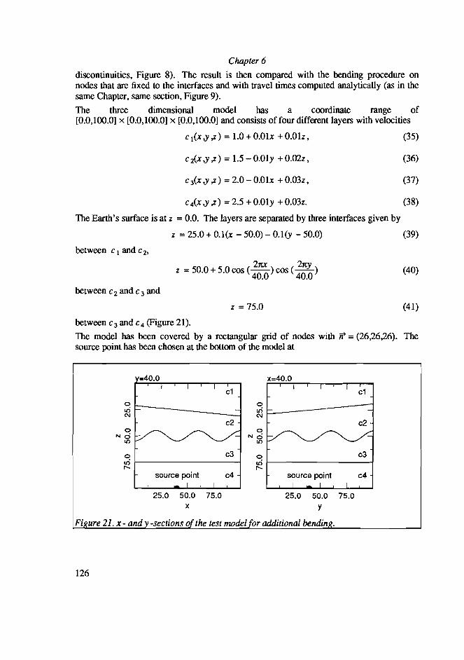
One important class of methods is formed by the ray methods Ray paths are the lines along which the seismic energy travels in the high frequency limit (Keller 1978) They are not physical but merely mathematical idealisations that are of great practical use When a source point has been indicated one can calculate rays leaving it in all directions by solving the appropriate differential equations Additional differential equations describe the amplitude along the ray (Cerveny 1987) The assumption that the medium is isotropic which means that the propagation velocity of the seismic energy is only dependent on the spatial position simplifies the theory because the ray paths are then perpendicular to the wave fronts Ray theory in anisotropic media in which the propagation velocity is also dependent on the direction of the ray is described by Vlaar (1968)

Generally the ray path between a source and a receiver is required There are essentially two methods to solve this two-point ray tracing problem shooting and bending (Julian and Gubbins 1977) Shooting is tracing ray paths from the source towards the receiver by solving the ray differential equations and by adjusting their initial directions trying to hit the receiver point Bending is starting with an arbitrary curve between the source and the receiver and perturbing it in such a way that the ray differential equations are satisfied or equivalently the travel time along it is extremal Both methods have their shortcomings for shooting it may be very difficult to find the correct initial direction because the trial ray paths may converge very slowly towards the receiver point for bending it is never certain whether the found extremal travel time curve is only a local extremum or the global extremum generally required These shortcomings may result in incomplete results or inadmissible computation times

The extremal travel time property of a ray path which is the variational equivalent of the ray differential equations was first formulated by Fermat in 1661 as a least time property It says that the travel time along a ray path is stationary that is it changes only to second order when the ray path is changed In this century Caratheodory showed that Fermats principle is indeed a least time principle in the sense that every sufficient small pan of a ray has a minimal travel time between its end points (Keller 1978) It provides an additional

vii

Introduction

check on a curve whether it is a real ray path or not and also gives rise to the application of minimisation techniques for finding seismic rays (Moser Nolet and Snieder 1992)

Another shortcoming of the shooting method that is inherent in ray theory is the occurrence of shadow wnes regions that cannot be reached by ray paths from one source point In shadow zones the high frequency assumption of ray theory breaks down because these zones are reached by waves with finite wave lengths or diffracted waves Shadow zones appear often in both global seismology and exploration seismics

In recent years methods have been developed to avoid these difficulties (Vidale 1988 1990 Qin et aJ 1990 Saito 1989 1990 Van Trier and Symes 1991 Matsuoka and Ezaka 1990 Podvin and Lecomte 1991) They construct travel time fields on a rectangular grid of nodes by solving the eikonal equation (Vidale 1988 1990 Qin et al 1990 Van Trier and Symes 1991) or by using Huygens principle (Saito 1989 1990 Podvin and Lecomte 1991) In any method the travel times on the grid points are constructed recursively from already known travel times starting with the source point and then expanding over the whole grid according to schemes that resemble expanding waves All of the methods construct the travel times from the source point to all other points simultaneously in one run of calculations This means that the two-point ray tracing problem is solved automatically for receivers at each grid point Therefore the grid methods are extremely efficient for the calculation of complete travel time fields Some of the methods however suffer from a lack of robustness in presence of high velocity contrasts where some waves may turn back to the source thereby conflicting with the propagation scheme of the calculations

The shortest path method developed in this thesis is similar to the above described grid methods but is based on Fennats principle and network theory The original idea came from Nakanishi and Yamaguchi (1986) who needed in their study of nonlinear inversion of first arrival times in an island arc structure a ray tracer that could find ray paths and travel times from one source point to a number of receiver points in any velocity model without difficulties The models they used consist of rectangular cells with a constant velocity in each cell Nodes are placed on the boundaries of the cells and connections between them are introduced when they are on the same cell (see Chapter 1 Figure la) Such a structure of nodes and connections is called a graph It becomes a network when weights are assigned to the connections When the weights are chosen equal to the travel time of a seismic wave along it that is equal to the ratio of their Euclidian length and the velocity in the cell between the nodes the shortest paths in the network can be interpreted as approximations to seismic rays thanks to Fennats principle One node can be indicated as a source node and the shortest paths from this node to all other nodes in the network together can be interpreted as the ray field As a pleasant circumstance all of the existing methods for the computation of shortest paths in a network construct the shortest paths and travel times along them from one source to the other points of the network simultaneously Therefore the resulting travel times are comparable to the travel times as obtained in the grid methods described in the previous paragraph However Nakanishi and Yamaguchi (1986) did not investigate the efficiency of the shortest path method nor did they examine other organisations of the networks

In the last thirty years a huge amount of literature was published on algorithms for computing the shortest paths in a network (Deo and Pang 1984) The most famous among them is Dijkstras (1959) algorithm Gallo and Pallottino (1986) describe modem versions

viii

Introduction

of the Dijkstra algorithm that are efficient enough to make the shortest path method competitive with other methods for forward seismic modeling As the network is an abstract mathematical object without explicit relation to the seismic model the shortest path method is very flexible in the sense that it applies for two as well as for three dimensional calculations without any modifications of the algorithm Moreover there has not been made any assumption on the spatial distribution of the nodes This means that any other ordering of the nodes than on cell boundaries as described above is possible Furthermore the availability of shortest path algorithms whose efficiency do not depend on the weights of the connections between the nodes of the network makes the shortest path method very robust even in complicated seismic models with large velocity contrasts The existence of a shortest path between two nodes is never in doubt Therefore it is no problem to find the shortest paths to shadow zones the network has only to be organised in such a way that the shortest path has a physical meaning

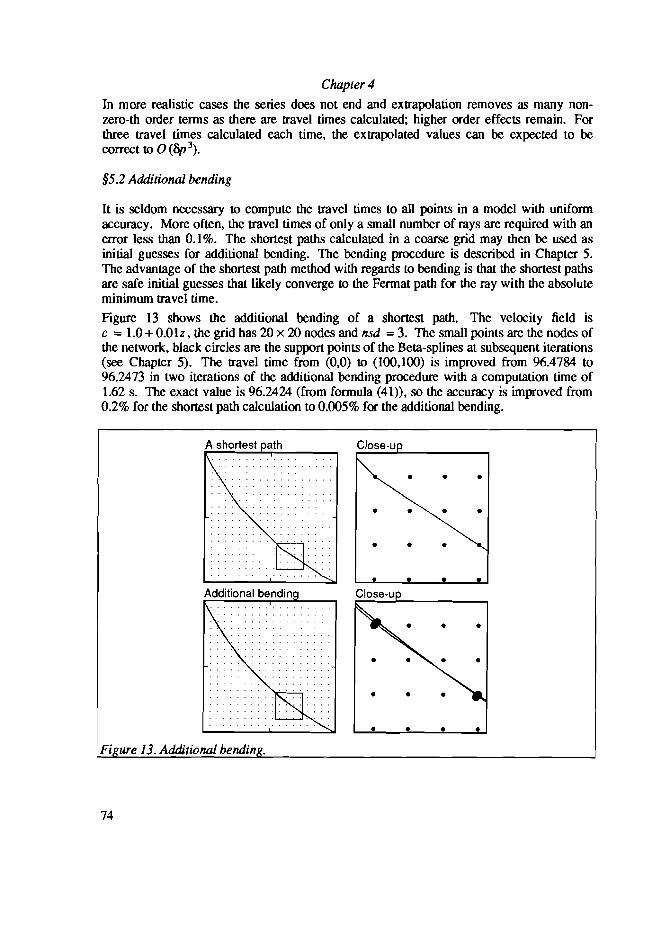
This thesis investigates the properties of the shortest path method for seismic ray tracing It has a twofold character it contains parts with a detailed description of the shortest path method and parts with practical geophysical applications The first chapter that was published as Shortest path calculation of seismic rays in Geophysics in January 1991 (Moser 1991) serves as an introduction The last three sections of the first chapter Shortest path algorithms and their efficiency Constrained shortest paths and reflection seismology and The accuracy of the shortest path method are introductions to Chapter 2 Chapter 3 and Chapter 4 respectively The reader who is exclusively interested in geophysical applications may safely skip these chapters and continue with Chapter 5 which contains newly developed ray bending methods that can be applied to refine individual results of the shortest path calculations Chapter 6 compares the shortest path method with other methods for forward modeling that are used in practice for exploration purposes The last two chapters show how the shortest path method can be applied to geophysical problems like the earthquake location problem (Chapter 7) and the stochastic analysis of global travel time data (Chapter 8)

The calculations of Chapter 1 were done on a GOULD PN9000 with one CPU 8 MB memory space and a Unix operating system In all other chapters the calculations were performed using one NS32532 processor of an Encore MM510 parallel computer with 25 Mflop (comparable to 42 Mflop on a SUN Sparc2) Unless otherwise stated physical quantities like distance time velocity and slowness were chosen dimensionless

ix

Shortest path calculation ofseismic rays

CHAPTERl

Shortest path calculation of seismic rays

Abstract

Like the travelling salesman who wants to find the shortest route from one city to another in order to minimise his time wasted on traveling one can find seismic ray paths by calculating the shortest travel time paths through a network that represents the Earth The network consists of points that are linked with neighbouring points by connections as long as the travel time of a seismic wave along it The shortest travel time path from one point to another is an approximation to the seismic ray between them by virtue of Fermats principle The shortest path method is an efficient and flexible way to calculate the ray paths and travel times of first arrivals to all points in the Earth simultaneously There are no restrictions of classical ray theory diffracted ray paths and paths to shadow zones are found correctly Also there are no restrictions to the complexity or the dimensionality of the velocity model Furthermore there are no problems with convergence of trial ray paths towards a specified receiver nor with ray paths with only a local minimal travel time Later arrivals on the seismogram caused by reflections on interfaces or by multiples can be calculated by posing constraints to the shortest paths The computation time for shortest paths from one point to all other points of the networks is almost linearly dependent on the number of points The accuracy of the results is quadratically dependent on the number of points per coordinate direction and the number of connections per point

Introduction

There are two traditional methods to compute seismic ray paths between two points in the Earth shooting and bending (Julian and Gubbins 1977) Shooting tries to find ray paths leaving one source point by solving the differential equations that follow from ray theory for different initial conditions until the trial ray arrives at the pre-assigned point Bending has Fermats principle as a starting point it tries to find a ray path between two points by searching the minimal travel time path between them

Both methods have serious drawbacks By shooting a fan of rays leaving the source one can obtain an impression of the wave field However convergence problems are known to occur frequently especially in three dimensions Also shooting will not find diffracted ray paths or ray paths in shadow zones where ray theory breaks down With bending one can find every ray path satisfying Fermats principle even a diffracted one but only for one sourcereceiver pair at a time and it is not certain whether the path has an absolute minimal travel time or only a local minimal travel time These drawbacks result in the low efficiency of the methods and the incompleteness of their results The problems are even more severe in three dimensional than in two dimensional ray tracing

This chapter has been published as

Moser TJ Shortest path calculation of seismic rays Geophysics Vol 56 No1 59-671991

1

Chapter 1

In this chapter a method is presented that avoids the disadvantages of shooting and bending It uses an idea of Nakanishi and Yamaguchi (1986) to approximate ray paths by the shortest paths in networks as a starting point Next methods are investigated to improve the efficiency of the search for the minimum time path and shows how it is possible to treat reflected arrivals in the same way

Network theory and shortest paths in networks are an abstract formulation of problems that appear in many different branches of science and technology They are usually of a discrete nature there are a finite number of objects and the exact solution of the problem can be found in a finite number of steps One example is the road map where the network consists of cities and connections between them one can ask for the shortest path from one city to another or the shortest closed circuit along all cities and so on A wide variety of network theory techniques is available Among them the methods based on the theory of shortest paths deserves special attention See Deo and Pang (1984) for a review of the literature on these subjects

One advantage of the shortest path method is that all shortest paths from one point are constructed simultaneously This conclusion follows from the nature of shortest path algorithms calculating one path costs just as little computation time as calculating all paths For instance it can be applied in the simulation of Common Shot Point gathers

Although a search that ignores the differential equations and even Snells law does not seem to be efficient at first sight seismic ray tracing can make direct practical use of the increased efficiency of shortest path algorithms Efficiency has been improved by several orders of magnitude in the last thirty years by introducing sophisticated data structures (Gallo and Pallottino 1986) The most efficient one for ray tracing can be selected by a simple comparison of the available algorithms The shortest path method is designed to find a good approximation to the globally minimal travel time and travel time path Therefore it is especially fit for applications in travel time tomography Later arrivals on a seismogram can only be computed if they can be formulated as constrained shortest paths For instance the shortest paths constrained to visit one point of a set of points that form a scatterer or interface approximate diffracted and reflected ray paths

Finally the abstract structure of a network has the consequence that there is no notion of dimensionality of the space so two and three dimensional ray tracing are possible with the same algorithms

sect1 Shortest paths in networks and seismic ray paths

This heuristic section precedes the more theoretical analysis and illustrates the possibilities of networks to represent approximate ray paths One important property of a seismic ray path is given by Fermats principle the ray path is a spatial curve along which the travel time is stationary The construction of a ray between a seismic source and a receiver can be based on this principle One could enumerate all curves connecting the source and the receiver and look for the minimum travel time curve Usually this is done by bending an initial guess of the ray path so that the travel time along it is decreased until stationarity is achieved The analogy between a seismic ray path and a shortest path in a network provides an alternative way to use Fermats principle

In this approach the relevant part of the Earth is represented by a large network consisting of points connected by arcs Each point or node is connected with a restricted number of

2


points in its neighbourhood but not with points that lie further away Therefore it is possible to travel from one node to another via the connections The network has indeed a resemblance with a three dimensional road map Like on a road map the connections between nodes have lengths This length is to be understood as a weight of the connection For example in the application to seismic ray tracing it is the travel time of a seismic wave between the two nodes In seismic ray tracing the connection will have equal length for both directions along it by virtue of the reciprocity principle In other applications of network theory the weight can be the electrical resistance in an electrical network the cost in an economical decision tree or whatever quantity that must be minimised in a discretised medium

When the length of an arc is chosen equal to the travel time of a seismic wave one can hope that the shortest travel time path between two nodes approximates the seismic ray path between them This hope will not be idle when the nodes of the network are distributed in such a way that almost any ray path can be approximated by paths through the network To this end regular distributions of the nodes and of the connections between them are introduced This is not only required to give reasonable approximations to seismic ray paths but results also in a considerable saving of memory space Two organisations of networks are used in this chapter to illustrate the shortest path method Both illustrations will be given only in two dimensions although the network theory does not impose any restriction on the dimensionality of the space All quantities are made dimensionless the horizontal distance x and the depth z range from 0 to 100

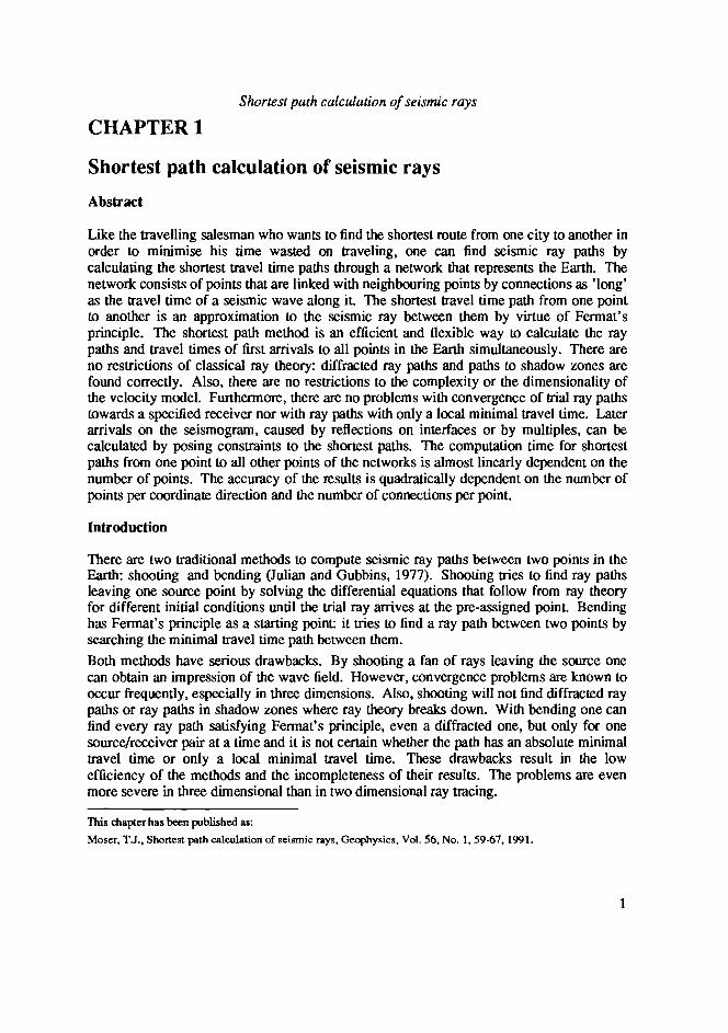
In the first example taken from Nakanishi and Yamaguchi (1986) the nodes are distributed regularly on the boundaries of rectangular cells in which the propagation velocity of seismic waves is constant (Figure 1) Two nodes are only connected when there is no cell boundary between them The travel time between two connected nodes is defined as their Euclidian distance multiplied with the slowness of the cell in between Figures 2a and 2b

Figure 1 Cell organisation of a network a) (left) Dashed lines cell boundaries Black circles nodes Solid lines connections b) (right) Shortest paths from one node to other nodes in a homo eneous model

3

Chapter 1

show the shortest paths in two networks The model of Figure 2a has a constant velocity of 10 so that the shortest paths approximate straight lines The model of Figure 2b has a (dimensionless) velocity distribution c =10 + OOlz so that the shortest paths approximate circular ray paths The cell organisation of networks is particularly suitable for the application to seismic tomography as in the paper of Nakanishi and Yamaguchi

The second example uses a rectangular grid of nodes in which each node is connected with the nodes in a neighbourhood of it The seismic velocity or slowness is sampled at the node locations The travel time between two connected nodes is defined as their Euclidian distance multiplied by the average slowness of the two nodes This organisation facilitates the drawing of contours of equal travel times and velocities and more important the introduction of interfaces Figure 3a shows a rectangular grid of 5 x 5 nodes each one connected with at most 8 neighbours In Figure 3b the shortest paths from the upper left node are plotted for a homogeneous model

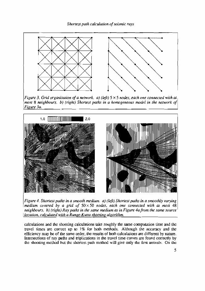
In Figure 4a a medium with velocities ranging from 10 to 20 is represented by a network of 50 x 50 nodes and at most 48 connections per node The shortest paths from one node at the left side of the model are plotted It can be seen that they converge in high velocity regions and try to avoid low velocity zones

The travel times along shortest paths to the 50 nodes at the right side of the model can be compared with travel times calculated with the shooting method for seismic ray tracing The ray paths in Figure 4b have been calculated by a numerical solution of the ray equation for 50 fixed initial directions with a fourth-order Runge-KUlla scheme (Stoer and Bulirsch 1980) No attempt has been made to reach a pre-assigned receiver point by a standard bisection method this will usually take about 5 times more computation time The ray paths are discretised into 25 points The travel times along the ray paths are correct up to 1 when compared to reference rays consisting of 100 points In this setting the shortest path

Figure 2 Shortest paths in cell networks with 10 x 10 cells and 10 nodes per cell boundary a) (ie t) Homo eneous model b) (ri ht) Linear velocit model c = 10 + OOIz

4


Figure 3 Grid organisation of a network a) (left) 5 x 5 nodes each one connected with at most 8 neighbours b) (right) Shortest paths in a homogeneous model in the network of Fi ure 3a

10~20

Figure 4 Shortest paths in a smooth medium a) (left) Shortest paths in a smoothly varying medium covered by a grid of 50 x 50 nodes each one connected with at most 48 neighbours b) (right) Ray paths in the same medium as in Figure 4afrom the same source location calculated with a Run e-Kutta shootin al orithm

calculations and the shooting calculations take roughly the same computation time and the travel times are correct up to 1 for both methods Although the accuracy and the efficiency may be of the same order the results of both calculations are different by nature Intersections of ray paths and triplications in the travel time curves are found correctly by the shooting method but the shortest path method will give only the first arrivals On the

5

Chapter 1

other hand the latter method has calculated the shortest paths to the 2450 other points in the same time Therefore a careful consideration of purpose accuracy and efficiency of the ray tracing problem is necessary The efficiency and accuracy of the shortest path method are given below

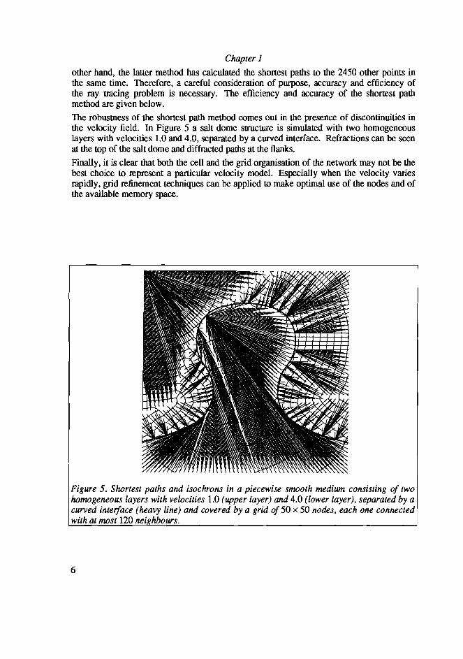
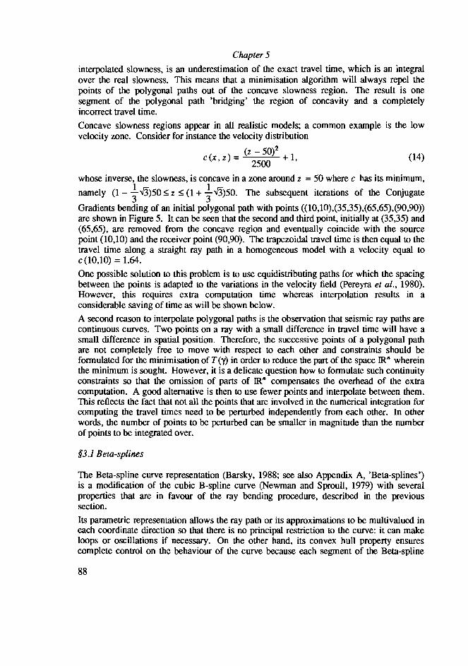
The robustness of the shortest path method comes out in the presence of discontinuities in the velocity field In Figure 5 a salt dome structure is simulated with two homogeneous layers with velocities 10 and 40 separated by a curved interface Refractions can be seen at the top of the salt dome and diffracted paths at the flanks

Finally it is clear that both the cell and the grid organisation of the network may not be the best choice to represent a particular velocity model Especially when the velocity varies rapidly grid refinement techniques can be applied to make optimal use of the nodes and of the available memory space

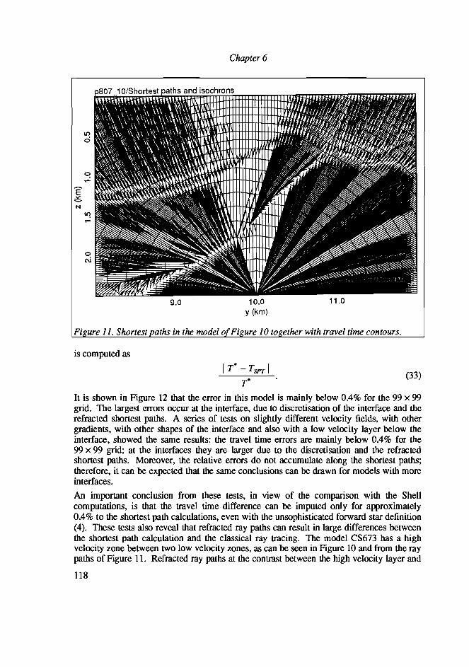
Figure 5 Shortest paths and isochrons in a piecewise smooth medium consisting of two homogeneous layers with velocities 10 (upper layer) and 40 (lower layer) separated by a curved interface (heavy line) and covered by a grid of 50 x 50 nodes each one connected with at most 120 nei hbours

6


sect2 Shortest path algorithms and their efficiency

For the description of shortest path algorithms the following notations and definitions are introduced G (N A) is a graph that is a set N containing n nodes together with an arc set A eN x N A network (G D) is a graph with a weight function DN x N ~ IR that assigns a real number to each arc D can be represented by a matrix (dij ) (Figure 6) For ray tracing purposes it can be assumed that D is symmetric by virtue of reciprocity dij =dji and nonnegative d ii =0 for i E N and dij ~ 0 for i j EN By convention dij =dji =00 denotes the case that the nodes i and j are not connected The forward star of node i FS (i) is the set of nodes connected with i All networks representing a velocity model used in this chapter are sparse it can be assumed that each node is connected only with the nodes in a small neighbourhood of it This means that the number of elements in the forward stars is bounded by a small number m with m laquo n and m = 0 (I) (n ~ 00)

A path is a sequence of nodes and connections succeeding each other The travel time along a path from one node to another is defined as the sum of the weights of the connections of the path A shortest path is a path with the smallest possible travel time It may not be uniquely determined as can be observed from Figure 1 The shortest paths from the source node s to all other nodes calculated with the available algorithms form a so called shortest path tree with its root at s and its branches connecting the other nodes There is one and only one way to reach a node from the source node through such a tree and there are no loops One consequence of the tree structure is that the shortest paths are described completely by an array of pointers prec (i) is the preceding node of i on the shortest path from s to i The source node s is by definition equal to its own predecessor A shortest path can be extracted from this array by repeating (j = prec (i) i = j until i = s The travel time along the shortest path from s to i is denoted with tt (i)

The shortest travel times from the point source s obey Bellmans (1958) equations

tt (i) = min(tt U) + dij ) i j E N (1a) J

subject to the initial condition

tt(s) = O (Ib)

s tt(j)

7

Chapter 1

The travel time to a node i is the minimum of the travel times to neighbouring nodes j plus the weight of the connection between both These equations follow easily from the observation that if tt (i) were not equal to Ii~(tt U) + dij ) there would exist a path with a

J

shorter travel time than tt(i) The node j that minimises ttU) + dij is exactly the preceding node of i on the shortest path from s to i j =prec (i) Bellmans equations suggest a scheme of constructing shortest travel times All initial travel times are equal to infinity except for the source node tt(s) = O It is now possible to repeat the nonlinear recursion

tt (i) = min(tt U) + dij ) (2)j E N

for all i E N until no more travel time can be updated This will certainly happen after many iterations The shortest paths from one node to all other nodes are then calculated In fact the available efficient algorithms calculate all shortest paths from one node simultaneously although not all that information may be useful

Dijkstras (1959) algorithm arranges an order of nodes to be updated so that after exactly n iterations the shortest paths are found The nodes are divided into a set P of nodes with known travel times and a set Q of nodes with travel times along shortest paths from s that are not yet known Initially P is empty and Q = N The minimum travel time node of Q is s It has a known travel time (tt (s) =0) so it can be transferred to P The travel times of all nodes connected with s all j E FS (s) are then updated in agreement with (2) An important fact is now that the node in Q with the smallest tentative travel time will no longer be updated Therefore it can be transferred to P and the nodes from Q connected with it are again updated This process of finding the minimum tentative travel time node transferring it to P and updating its forward star is repeated exactly n times The complete shortest path tree is then constructed Thus Dijkstras algorithm can be formulated as follows

Dijkstras algorithm 1 Initialisation

Q=N tt(i)= 00 for all i EN P =0 tt(s) = 0

2 Selection find i E Q with minimal travel time tt (i)

3 Updating ttU)= min(ttU)tt(i) + dij for all j E FS(i)nQ transfer i from Q to P

4 Iteration check if P =N stop else go to 2

Dijkstras algorithm is the classical algorithm for the computation of shortest paths but alternatives have been developed that are several orders of magnitude more efficient To consider the computational efficiency of Dijkstras algorithm the number of operations can be counted The initialisation step requires n operations to initiate the travel times The first time the selection step requires n comparisons Each iteration the number of required comparisons drops one because the number of elements of Q decreases by one The updating costs at most as many operations as there are elements in FS (i) namely m

8


Therefore the total number of operations is

n + (n - 1) + (n - 2) + + 1+ m x n = 0 (n 2) (n ~ 00)

which implies that the computation time is essentially quadratically dependent on the number of nodes

The selection of the minimum travel time node (step 2) turns out to be the most time consuming step of the algorithm because at each of the n iterations the entire set Q of tentative travel time nodes must be scanned The scanning could be omitted if the travel times in Q were completely ordered in a waiting list The minimum travel time node could be found immediately as it would be the first of the waiting list However each updating requires the updated node to be shifted to its right position in the waiting list This costs again 0 (n) comparisons per iteration Consequently a complete ordering does not improve the quadratical dependence of the computation time on the number of nodes

An alternative was introduced by Johnson (1977) and described by Gallo and Pallottino (1986) First all nodes in Q with tentative travel times 00 can be removed from the waiting list as they will never be the smallest The rest of the nodes in Q are then partially ordered in a so-called heap A heap is an array of elements a (i) i = I n such that

a (i) 5 a (2i) (3a)

and

a (i) 5 a (2i + 1) (3b)

for i = 1 n 2 Consider for instance the travel times

77800075899790930070 1019987007491

After the removal of infinite travel times these can be ordered in a heap as

707574808777938910199979091

The advantages of the heap structure come out when these numbers are represented as a tree (Figure 7) The conditions (3) are visualised in that each number is smaller than or equal to the two numbers just below it It can be seen that the number of elements in one generation or horizontal layer grows exponentially with the height of the heap Therefore there are only logn generations for a heap of n nodes The minimum travel time can be found immediately it is the uppermost number When some finite travel time is updated it may violate the conditions (3) so it must ascend or descend to restore the heap structure Removing the minimum travel time node from the heap and adding an infinite travel time node whose travel time has become finite can also be formulated as descents and ascents These cost at most logn operations The total number of operations for the calculation of a shortest path tree is now

logn + log(n - 1) + + log1 + m x n = 0 (n logn ) (n ~ 00)

which is much faster than the quadratical computation time of the original Dijkstra algorithm

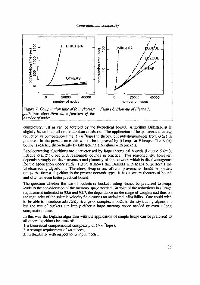
The computational times are plotted for four different shortest path algorithms on a series of networks in Figure 8 The calculations were done on a GOULD PN9000 with one CPU 8 MB memory space and a Unix operating system Only the shortest path calculation times

9

Chapter 1

Fijure 7 The tree structure ofa heap

2000 COMPUTATION TIMES HEAP DIJKSTRA LOUEUE LDEOUE

1750

_1500

~ 51250 o ill

~1000 ill ~ 750 tl o 500

250

10000 20000 30000 40000

Figure 8 Computation times of various shortest path algorithms as a function of the number 0 nodes

NUMBER OF NODES

are measured not the input and output of data The networks are cell networks with 10 nodes per cell boundary and the number of cells in both x and z directions increasing one by one from 1 to 100 For each of the hundred networks one shortest path calculation is done for the four different algorithms the original Dijkstra algorithm (DUKSTRA) the Dijkstra algorithm with Q organised as a heap (HEAP) and an alternative of Dijkstras algorithm with Q organised as a queue (LQUEUE) and as a so called double ended queue (LDEQUE) See Gallo and Pallottino (1986) for details on LQUEUE and LDEQUE The

10


original Dijkstra algorithm appears to have indeed a quadratical computational complexity In the application to seismic ray tracing LQUEUE and LDEQUE are not as fast as is promised in the literature on shortest paths HEAP is the most efficient algorithm it has a computation time that is almost linearly dependent on the number of nodes This is caused by the sparseness of the networks used in ray tracing the heap size is much smaller than the set of aU nodes during the whole process

sect3 Constrained shortest paths and reflection seismology

A restriction to seismic ray tracing with the shortest path method is that only the absolutely shortest paths are found Later arrivals on the seismogram like reflections and multiples caused by discontinuities in the spatial velocity distribution do not travel along the shortest path between the source and the receiver and will not be found by a simple shortest path algorithm Yet they are of scientific and economic importance because they contain additional information about the Earths structure Therefore it is necessary to impose a constraint on the shortest paths This constraint can be formulated as the demand to visit a specified set of nodes that lie on the interface

The solution to the constrained shortest path problem is as follows First all shortest paths from the source node s to all other nodes are calculated with Dijkstras algorithm The

Figure 9 Constrained shortest paths a) The primary field in a medium with constant velocities 10 (upper layer) 12 (middle layer) and 14 (lower layer) and a grid network of 50 x 50 nodes each one connected with 100 nei hbours

11

Chapter 1

travel times of the nodes on the interface are then selected remembered and ordered in a heap All other travel times are again set to infinity The set Q is re-initialised to N and P is re-emptied Dijkstras algorithm is then restarted at step 2 the selection step The resulting travel times are the travel times of shortest paths that are constrained to visit the interface node set

Consider Figure 9 to see how this works A model is generated that consists of three homogeneous layers with velocities 10 12 and 14 separated by curved interfaces (heavy lines) The shortest paths from one source point at the Earths surface are shown in Figure 9a It is known a priori that points with a non-zero scattering coefficient are real physical scatterers Nodes on interfaces or more precisely nodes with neighbours with a much different velocity are real scatterers so they should reflect shortest paths Therefore they are selected and gathered in a new source node set before restarting the algorithm The result is shown in Figure 9b The shortest paths in the uppermost layer are reflections on the first interface They satisfy approximately the law of incidence and reflection The paths in the second layer are the same paths as the unconstrained shortest paths in Figure 9a This is no surprise because these paths automatically satisfy the constraint to visit one of the interface nodes It can be seen that Snells refraction law holds as far as the network structure permits The procedure of collecting scattering nodes in a new source node set and restarting the algorithm can be repeated ad infinitum so one can calculate as many multiple reflections as desired Figure 10 shows the continuation of the constrained shortest paths of Figure 9b now under the constraint to visit the second interface The paths are the shortest ones that visit the first interface first and next the second interface In

12


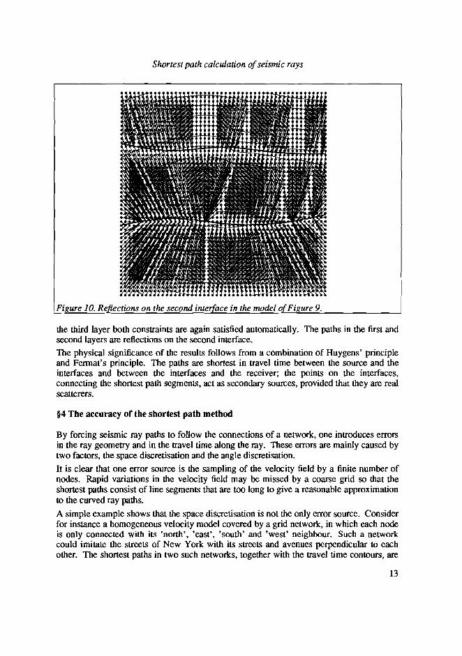
the third layer both constraints are again satisfied automatically The paths in the first and second layers are reflections on the second interface

The physical significance of the results follows from a combination of Huygens principle and Fermats principle The paths are shortest in travel time between the source and the interfaces and between the interfaces and the receiver the points on the interfaces connecting the shortest path segments act as secondary sources provided that they are real scatterers

sect4 The accuracy of the shortest path method

By forcing seismic ray paths to follow the connections of a network one introduces errors in the ray geometry and in the travel time along the ray These errors are mainly caused by two factors the space discretisation and the angle discretisation

It is clear that one error source is the sampling of the velocity field by a finite number of nodes Rapid variations in the velocity field may be missed by a coarse grid so that the shortest paths consist of line segments that are too long to give a reasonable approximation to the curved ray paths

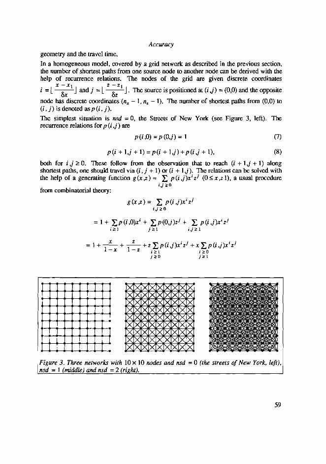
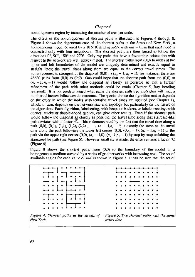
A simple example shows that the space discretisation is not the only error source Consider for instance a homogeneous velocity model covered by a grid network in which each node is only connected with its north east south and west neighbour Such a network could imitate the streets of New York with its streets and avenues perpendicular to each other The shortest paths in two such networks together with the travel time contours are

13

Chapter 1

shown in Figure II The network of Figure Ila has 10 x 10 nodes the network of Figure lIb 50 x 50 nodes It is obvious that increasing the number of nodes does not improve the accuracy of the results in both networks the travel time contours are straight lines instead of circular wavefronts One could hope that the shortest paths would approximate the straight ray paths in the homogeneous model but they are far from unique so a great number of paths have the same (shortest possible) travel time

Therefore it can be concluded that the error in the travel time and the ray geometry depend on the number of nodes and the number of connections per node When the average Euclidian distance between two connected nodes is denoted with ~x and the average smallest angle between two connections leaving one node with 0Ilgt the travel time error E = T (exact) - T (approximate) obeys an asymptotical relation of the type

E = 000 + (l1O~X + 0(J101lgt + Clw~x2 + (ll1~XOllgt + aoz0llgt2 + (4)L (lij ax i ampjti (~x OIlgt ----) 0)

j + j gt 2

where (lij are numbers that depend on the variation of the velocity field and the network It can be shown that

aoo = (l1O = 001 = O

This means that the travel times are correct up to the second order in the space and angle discretisation This result will not be proved here but it can be illustrated in a linear velocity model Such a model can be thought to be more or less representative for sufficiently smooth models as they can be approximated by linear velocity regions for small Bx Effects of the discretisation of nonsmooth models are visible at the interfaces in Figures 9 and 10

The calculations of Figure 2b are done for different space and angle discretisations The travel times in the velocity field c = 10 + OOlz are computed in a series of cell networks with n~ the number of cells in the x and z direction increasing from 2 to 50 with step I

Fi ure 11 Shortest aths in the streets 0 New York a) 10 x 10 nodes b) 50 x 50 nodes

14


and nr the number of nodes per cell boundary for each nJ increasing from 2 to 15 nr is a

measure for ~ and nJ for S~ The travel times are compared to the analytical formula

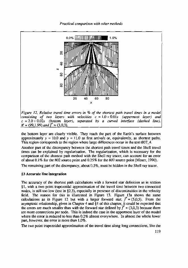
for travel times in constant gradient media (terveny 1987) The absolute difference is averaged over all nodes further away from the source than 10 and divided by the computed travel time This average relative travel time error is plotted logarithmically in Figure 12 It can be seen that the error is smaller than 01 for moderately large networks This result can be compared with the computational complexity by counting the total number of nodes n as a function of nJ and nr

n = 2nr (nJ + n)

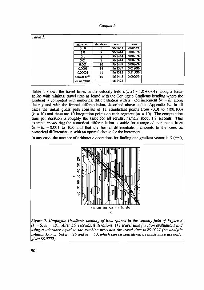
For a cell network of 30 x 30 cells and 10 nodes per cell boundary the average relative travel time error is 00939 The total number of nodes is 18600 and the CPU time for this calculation is 317 seconds for the LDEQUE algorithm and 322 seconds for the HEAP algorithm (see Figure 8) The logarithmic plot of the average relative travel time error

(Figure 17) shows that the error curves tend to a ~ relation for nJ ~ 00 This points to nr

the fact that CXoo = 001 = O (XIO = 0 can be illustrated in the same way

error curvesnx=2(1 )50

-100 -_--1-- bullbullbullbull

-cshyg -200 ~ o T

~ -300

025 050 075 100 125 150 log10 (nr)

Figure 12 The travel time error as a function of the number of nodes and the number of connections er node in a linear veloci model covered b cell networks

15

Chapter 1

Conclusions and discussion

The shortest path method is a flexible method to calculate seismic ray paths and shortest travel times It can be easily coded in FORmAN because of the general abstract formulation of network theory There is no need for extra software for complicated structures nor for three dimensions The method constructs a global ray field to all points in space so there are no problems with the convergence of trial rays towards a receiver The method finds the absolute minimal travel time path instead of getting stuck in a local minimal travel time path Later arrivals on the seismograms can be found by an extra run of the shortest path algorithm The shortest path method has a computation time that is almost linearly dependent on the number of nodes Its accuracy is quadratically dependent on the number of points per coordinate direction and the number of connections per point Even when this may not be enough for a few number of rays the shortest paths are good initial guesses for additional bending The multiple ray paths that can be seen in Figure 4b cannot be modeled with the shortest path method at least not by using the suggestions of the section on constrained shortest paths and reflection seismology

16

Computational complexity

CHAPTER 2

On the computational complexity of shortest path tree algorithms

Introduction

Many methods for forward modeling suffer from efficiency problems This is due partly to the source receiver configuration partly to the complexity of the velocity model or the existence of large velocity contrasts These problems cause unacceptable computation times for sometimes trivial results Therefore a new method for seismic ray tracing can be justified among other things by its computational efficiency In this chapter the efficiency of ray tracing by means of the shortest path method is analysed It is shown that algorithms exist with a computation time which is almost proportional to the number of nodes and the number of connections per node in the networks This implies a proportionality with the volume of the model and with the desired accuracy of the ray paths and the travel times along them (see Chapter 4 Accuracy of ray tracing by means of the shortest path method) A favourable property of all shortest path algorithms is that they construct the shortest paths from one source point to all other points with approximately the same computational effort as to only one receiver point The fact that all ray paths and the total travel time field are constructed simultaneously makes the shortest path method competitive with the shooting method for seismic ray tracing which can have serious problems to make a series of trial ray paths converge toward the correct receiver It is also shown that algorithms exist whose computation time does not depend on the weight of the connections between the nodes or equivalently the range of the velocity in the model Other methods whose computation time is dependent on the range of velocities in the model like the finite difference solution of the wave equation have problems with large velocity contrasts near fault zones

The reviews of Deo and Pang (1984) and Gallo et aI (1982) on the huge amount of literature on shortest path algorithms are used gratefully Due to their work it is possible to restrict attention to the special case of sparse undirected networks with nonnegative weights and to concentrate on the application on seismic ray tracing The explanation of the algorithms follows the ideas argued in the paper of Gallo and Pallottino (1986) Denardo and Fox (1979) Fox (1978) and Dial et al (1979) give insight in the data structures applied in the algorithms

In the first section notations and definitions are introduced and it is shown how efficient an algorithm must be to compete with other ray tracing methods The algorithms available are classified in sect2 The algorithms are discussed in the sections sect3 and sect4 using the classification of sect2 as a guideline To confirm and amplify some theoretical evidence the results of an experiment on networks of realistic sizes are presented in sect5 In the last section it is concluded that in general cases the algorithm of Dijkstra implemented with so called heaps works the fastest of all if one takes into account the memory space requirements and the flexibility with regard to irregular seismic velocity fields

17

Chapter 2

sect1 Definitions and preliminary considerations

sect11 Notations

The following definitions and notations are used

A graph G (N A) is a node set N containing n nodes and an arc set A eN x N A network (GD) is a graph with a weight function DA ~ JR This function assigns to each arc (i j) E A a real number the weight which is the travel time from i to j in the special case of seismic ray tracing D can be represented by a matrix (djj ) The assumption is made that G is undirected which means that D is symmetric (djj = djj ) This assumption is due to the reciprocity of travel times with respect to source and receiver Further D is nonnegative dii =0 for each i and djj ~ 0 for each i j EN

a is the number of arcs in A corresponding with real connections Pairs of nodes that are not connected get a travel time equal to infinity (i j) d A ~ djj = 00 Infinity is just a large number far exceeding each possible other quantity

The forward star of node i FS (i) = (j E N I djj lt 00) is the set of nodes j connected with i This term originates from the case in which D is not symmetric and a backward star has to be defined as well The maximum number of elements of a forward star is denoted with m The letter Q is reserved to denote the set of candidate nodes for updating for which shortest travel times will be calculated in future iterations q = I Q I is the number of such nodes the vertical bars I I are used to denote the number of elements of a set

s is used to denote the source node from which the shortest path tree is calculated prec (i) is the preceding node of i that is the first node on the shortest path from i to s The travel time of i along that shortest path is denoted as It (i)

An asymptotic relation which is used to describe the computational complexity CC of an algorithm as a function of some graph related quantity is denoted with Landaus symbols

f(x) =O(g(x)) (x ~xo) means that I flaquoX) I is finite for x ~xo and f(x) =o(g(x)) g x)

(x ~ xo) means lim f laquox)) =O When Xo =00 as is mostly the case (x ~ xo) will be z-+zgx

skipped

rx l means the smallest integer which is greater than or equal to x LxJ is the greatest integer smaller than or equal to x

sect12 Comparison with other ray tracing algorithms

Seismic ray tracing with one source corresponds with the construction of the shortest path tree with the source node as source rather than with the construction of only the shortest path between one pair of nodes This follows from the fact that finding the shortest path between nodes i and j implies for each existing algorithm finding all shortest paths between i and j Thus solving the shortest path problem for two nodes at the extreme ends of a network is the same as constructing the whole shortest path lIee for one of the nodes When one seismic ray is traced it is a little more effort to go on and trace all rays

18


In this way it can be said that ray tracing by network simulation means simultaneous calculation of all rays and the whole travel time field

In order to compete with other ray tracing algorithms such as shooting and bending it must be shown that there is a solution to the shortest path problem which can be reached in a sufficiently small amount of time and number of operations in particular when the network size grows to infinity (Infinity in the sense of very large n) In addition it must be shown that with that amount of wotk a comparable result is obtained From the preceding it is clear that ray tracing in graphs provides other and more though less accurate infonnation than ray tracing by shooting or bending methods which only calculate one ray path each time It is possible to store the travel times along that ray path but to calculate the whole travel time field (that is in n nodes) needs n times running the shooting or bending algorithm The results however are more accurate

To avoid this discussion at this point it would be preferable to find an algorithm which runs an order of magnitude faster than the faster one of shooting and bending to n points in space Julian and Gubbins (1977) claim that bending is ten times faster than shooting and give an asymptotic relation for the number of operations to calculate one ray namely o (k 3

) if the ray is detennined by k points When n points or nodes are distributed homogeneously in a volume one line will contain approximately 0 (n 113) As a consequence calculating one ray by bending costs 0 ((n 113)3) = 0 (n) operations so calculating all n rays costs 0 (nn) = 0 (n 2) operations The conclusion is that a shortest path algorithm must run in 0 (n 2) time to beat other ray tracing algorithms even in the crude complexity estimation above

sect13 Topology

In the literature on network theory and shortest path problems much attention is paid to the density and the topology of the network and their implications for the computational complexity In the application on ray tracing with D symmetric and nonnegative two notions are of interest sparseness and planarity A network is called sparse if

n lt a laquo ~ n (n - 1) (n is the number of nodes and a the number of arcs) It is called

dense if n laquoa lt ~ n (n - 1) and complete if a = ~ n (n - 1) each pair of nodes is

connected by an arc with a finite weight in the latter case If a lt n the network is not connected and it is possible to point out a pair of nodes between which there does not exist a path at all let alone a shortest path A class of networks satisfying a = g (n) for some function g is said to have the same density In the application on seismic ray tracing a 5 mn for each graph with m a small constant integer (msl00) Sparseness means that the forward stars FS (i) are small which will appear to be crucial

A network is called planar if it can be mapped on IR2 with possible scaling of the weights in such a way that no intersection of arcs occurs The graphs used to represent seismic models are never planar except from the case where the model is two dimensional and each node is only connected with its direct neighbours The computation time of some algorithms depends on whether or not the graph is planar

19

Chapter 2

sect14 Complexity bound estimation

In the following sections algorithms are to be compared with each other on the ground of the asymptotic relation 0 if (n)) which predicts the order of magnitude of computation time as a function of n A historical review like Tarjans (1978) shows a search for the most efficient algorithms for graph theoretical problems The question whether there is an absolute lower bound for the theoretical complexity for instance 0 (n) will not be treated here It is more important to note that theoretical complexities are worst case bounds which refer to extremely unrealistic cases A worst case bound can be stated when a special (pathological) network can be indicated for which the shortest path algorithm runs that long computation time Therefore it is more suitable to give an expected case bound (Noshita 1985) As this demands a whole machinery of statistical analysis this will not be done here but it will be shown experimentally if an algorithm with a very bad worst case bound has a reasonable expected case bound

sect15 Storage requirement

Apart from computation time one must take care of the memory space needed to execute an algorithm It may be possible to design arbitrary efficient algorithms but with an undesirable memory space requirement Most methods need kn numbers where k 5 5 stored in arrays including tt (n) and prec (n) In literature the forward stars of each node or the whole matrix D are often stored This is not feasible in the application on seismic ray tracing because that would need a real numbers where a raquo n even if a = 0 (n) The alternative is to make an implicit definition of the forward stars This is possible and easy when the nodes have been well ordered The elements of the forward star can then be found by enumerating the neighbouring nodes Also when the connections of the forward stars have a constant geometrical shape standard weights can be stored so that the real weights can be calculated by only one multiplication

sect2 Classification of shortest path tree algorithms

There is no complete agreement in the literature on shortest path algorithms about how to classify them Most authors like Deo and Pang (1984) distinguish between labelcorrecting and labelsetting methods but Gallo and Pallottino (1986) object that some algorithms are labelcorrecting or labelsetting according to the kind of graph They distinguish between lowest-first search breadth-first search and depth-first search algorithms All species are different in the way they treat the set of nodes whose travel times are yet to be changed Most of them are common so far as they are based on one prototypic algorithm This algorithm gives the unique solution to the Bellmans (1958) equations

tt(i) = 1~(djj + tt(j)) i j E N J

i t s (1)

This is a set of nonlinear equations that subject to the initial condition

tt(s) =0 (2)

uniquely determines the travel times tt (i) of all nodes i along shortest paths from source node s The prototypic algorithm to solve this is as follows (Gallo and Pallottino (1986) )

20


Algorithm SPf 1 Initialisation

for allj E N - s tt(j) = 00

prec(j) =j for j = s

tt(j) = 0 prec(j) = s

set Q =s 2 Selection and updating

for some i E Q Q=Q-i

for all j E FS(i) with tt(i) + dij lt tt(j) tt(j) = tt(i) + dij prec(j) = i Q =Quj

3 Iteration if Q 0 goto 2 else stop

Each time a node j is updated it gets a new label tt (j) = tt (i) + dj because tt (j)(new) lt tt (j)(old) so tt (j)(new) is a better approximation to the solution of Bellmans equations Q is the set of candidate nodes for updating so if Q is empty the process is finished

sect21 Labelsetting versus labelcorrecting

According to the treatment of the set Q of candidate nodes for updating an algorithm is called labelsetting or labelcorrecting When each node after its removal from Q is added to a set of permanently labeled nodes P and will stay there during the rest of the iterations the algorithm is labelsetting When there is no such set the algorithm is labelcorrecting even in the last iteration each node could be relabeled

A modification of the classification of labeling algorithms of Deo and Pang (1984) is given in Figure 1 In the following each of these methods will be discussed and each will be given an asymptotic relation for its computational complexity

sect22 Classification with respect to search methods

In Gallos and Pallottinos (1986) classification a distinction is made between lowest-first search algorithms depth-first search algorithms and breadth-first search algorithms each differing in the way they select a node from the set Q of candidate nodes for updating When as in the lowest-first search case the node i with the shortest travel time is selected and its forward star FS (i) is updated i itself does not need to be updated any more during the rest of the iterations For that reason all lowest-first search algorithms are labelsetting provided that the weight matrix D is nonnegative as in the application on seismic ray tracing for instance Johnson (1973) shows that the Dijkstra algorithm is labelsetting when D is nonnegative but labelcorrecting in the general case Labelcorrecting algorithms which implement Q as a queue are breadth-first search implementation as a stack is depth-first

21

Chapter 2

labeling algorithms

buckets ordered in a heap

search and the use of double-ended queues is a mixture of both

sect3 Labelsetting algorithms

sect31 Dijkstras method

In Dijkstras method (1959) Q is implemented as a totally unordered set of nodes with temporary travel times yet to be updated This means that at each iteration the whole Q has to be scanned to find the minimum travel time node However for a nonnegative weight matrix D it is certain that the solution is reached in n iterations because each time Q is reduced with exactly one node The algorithm is as follows

Algorithm DIJKSTRA 1 Initialisation

for allj EN - s ttGgt = 00

preca) =j for j = s

tta) = 0 preca) = s

setQ =N 2 Selection and updating

find i E Q such that tt(i) = min tta)Je Q

for all j E FS(i) with j E Q and tt(i) + dlJ lt ttm tta) = tt(i) + dij

22


prec(j) =i Q =Q- il

3 Iteration ifQ- (2) goto 2 else stop

Scanning Q at each iteration costs q = I Q I comparisons updating I FS (i )nQ I comparisons and additions In the first iteration q = n next n - 1 and so on until q = 0 in each iteration IFS (i )nQ I ~ m The result is

1CC = Lq +nm = 2n(n + 1)+mn = o(n 2) (3)

qIJ

Dijkstras algorithm requires three n -vectors one for tt (n ) one for prec (n) and one for the implementation of Q in all 3n memory places

sect32 Linked lists

The preceding argument makes it clear that scanning the whole set Q of temporary labeled nodes to find the minimum labeled node is the most expensive operation To save time it is necessary to impose some structure on Q First exclude from Q all nodes with travel time infinity these nodes are not to be considered when searching for the minimum travel time node so there is no need looking for them Only when a node gets a finite label it should be added to Q Then as suggested by Yen (1970) Q can be ordered as a linked list in the following way Let

tt(Q(1raquo~tt(Q(2raquo~ ~tt(Q(qraquo (4)

then define head =Q (1) tail =Q (q) s(QUraquo=QU+l)forj =1middotmiddotmiddotq-l p(QUraquo = QU -1) for j = 2middotmiddotmiddot q p(Q(Iraquo = s(Q(qraquo =-1 p U) = sU) = ~ when j fi Q

Two new arrays p (n) a predecessor array and s(n) a successor array are introduced pU) is a pointer to the preceding node of j in Q that is the node with the longest travel time ~ tt (j) and sU) is a pointer to js following node in Q that is the node with the

-1s (1) -~ s(2) - ~ s(3) -- -~ s(l -1)-- s (1) -~

-1 - p(l) p(2) f- p (3) - f- p(l -1) - p(l)

Fi ure 2 Linked list

23

Chapter 2

shortest travel time ~ tt(j) p(j) = -1 and s(j) = -1 mean that j is the head and the tail of the list respectively ~ is some other non-element symbolp(j) = s(j) = ~ cent=gt j fi Q The element of Q with minimum travel time is obtained by simply setting i = head

Deleting this elementi from Q reads head = s(i)p(head) = -1 s(i) = p(i) =~

Adding a node j with former travel time tt (j) = 00 to Q reads s (tail) = j p (j) = tail s (j) = -1 tail = j which has to be followed by moving a node j to its right place

repeat interchange j and pO) correct p and s appropriately

until tt(pO) ~ ttO) The whole algorithm thus becomes

Algorithm DUKSTRA-LIST 1 Initialisation

for aIIj E N - (s) ttO) =00

prec(j) =j p(j) = s(j) = ~

for j = s tt(j) = 0 prec(j) = s p(j) = s(j) =-1

set Q = (s] head = tail = s

2 Selection and updating i = head remove i from Q for all j E FS(i) with tt(i) + dlj lt tt(j)

tt(j) = tt(i) + dlj prec(j) = i if j fl Q add j to Q move j to right place in Q

3 Iteration ifQ 0 goto 2 else stop

(cf algorithm DIJKSTRA) The number of iterations of DIJKSTRA-LIST is the same as DIJKSTRA n Finding the minimum travel time node of Q costs 0 (1) operations now and updating FS (i) still 0 (m) Moving j to its right place costs 0 (q) operations but often much fewer because it will seldom happen that j has to move through the whole Q to find its right place the tentative travel time of j would then be infinite before the updating and the smallest of Q after the updating Yet this is not impossible so the worst-case bound is 0 (n) The result is

CC = (1 + m + n)n = 0 (n 2) (5)

The required memory space is four n -vectors namely tt (n ) prec (n ) p (n) and s (n) It can be concluded thal the use of a list causes no significant acceleration of DIJKSTRA

24

Computational complexity sect33 Heaps

Numerous authors make use of heaps in order to speed up the search of the minimum travel time node in Q and to maintain the structure of Q after deleting the minimum element and after updating nodes For technical details see Aho Hopcroft and Ullman (1974) and Knuth (1968) A heap is defined as an array of real numbers (aj)= with the property that aj ~ au and aj ~ au + Heaps can be viewed as binary trees turned upside down with the smallest element on top For example the array (54461827133) can be ordered in a heap as (24345761813) and in a tree as in Figure 3 The top element of the heap is called the root for each triple (aj au au + ) aj is the parent au and au + are sons If an element has no sons it is called a leaf

Some simple properties of heaps can be derived For a given array (a j )= h gt 2 there is no uniquely determined heap Each element of a heap is less or equal to the elements of thej subheap on top of which it is A heap with k generations has at most L i-I = 2j - 1

j = elements only the e generation may not be filled Consequently a heap with h elements has r 210g(h + 1)1 generations The profit of the use of heaps is based on this property because when some element aj has been changed and must be moved to its right position at most r 210g(h + 1)1 descents or ascents are needed

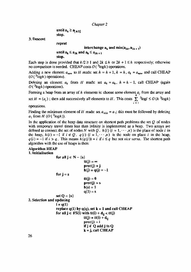
Let H be a heap with h elements aj and with one element aj changed in value Due to this change H may be not a heap any more so it must be restored as follows

Algorithm CHEAP 1 Ascend or descend

if ak lt l kl2J goto 2 if ak gt ~k or ak gt a2k + 1 goto 3 else stop

2 Ascent repeat

interchange ak and 3t kl2J

2

25

Chapter 2

until ak ~ 8t kl2J stop

3 Descent repeat

interchange 8k and min(a2k a2k + 1) until ak ~ a2k and ak ~ a2k + 1

stop

Each step is done provided that k 12 ~ 1 and 2k ~ h or 2k + 1 ~ h respectively otherwise no comparison is needed CHEAP costs 0 ( 210gh) operations

Adding a new element anew to H reads set h = h + 1 k = h ak = aMM and call CHEAP (0 (210gh) operations)

Deleting an element ak from H reads set ak = a h = h - 1 call CHEAP (again o (210gh) operations)

Forming a heap from an array of h elements is choose some element aj from the array and

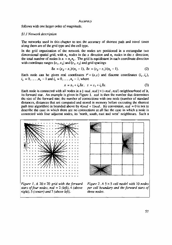
set H = (aj) then add successively all elements to H This costs ~ 210gi ~ 0 (h 210gh) i = 1

operations

Finding the minimum element of H reads set amin = a 1 this must be followed by deleting a1 from H (O( 210ghraquo

In the application of the heap data structure on shortest path problems the set Q of nodes with temporary travel times less than infinity is implemented as a heap Two arrays are defined to connect the set of nodes N with Q h (i) (i = 1 n) is the place of node i in the heap h(i) = -1 if i fI Q q (i) (i = 1 n) is the node on place i in the heap q (i) = -1 if i gt q This means h (q (iraquo = i if i ~ q but not vice versa The shortest path algorithm with the use of heaps is then

Algorithm HEAP 1 Initialisation

foralljE N- (s) tt(j) =00

prec(j) =j h(j) = q(j) =-1

for j =s tt(j) =0 prec(j) =s h(s) = 1 q(1) =s

set Q =(s) 2 Selection and updating

i = q(1) replace q(1) by q(q) set k =1 and call CHEAP for all j E FS(i) with tt(i) + diJ lt tt(j)

tt(j) = tt(i) + diJ prec(j) = i if j It Q add j to Q k = j call CHEAP

26

CompUlational complexity

3 Iteration ifQ F- 0 goto 2 else stop

The computational complexity is

CC = (210gq + m + 210gq ) n = 0 (n 210gq ) ~ 0 (n 210gn ) (6)

Just like DUKSTRA-LIST four n -vectors are needed tt (n) prec (n) h (n) and q (n)

sect34 ~-heaps

A generalisation of the heap structure is the ~-heap A ~-heap is defined as an array (ai )=1 with the property that ai ~ afi ai ~ afi + 1 ai ~ af(i + 1) -1 for each i provided that each index exists Each element has at most ~ sons The operations on heaps earlier described change accordingly Updates and insertions cost 0 ( 1310gh) and deletions cost 0 (~ 1310gh) Thus running the shortest path algorithm with ~-heaps costs o (~n flogn) operations in the worst case The function CC (~ n) = ~n flogn achieves its minimum for ~ =e =27182818 so the most suitable choice of ~ would be ~ =3 The gain of efficiency by taking 3-heaps instead of 2-heaps is

3n 310gn = 1310g2 09463949 (7)2n 210gn 2

which is only 55

Noshita (1985) proposes a LClog 2a J-heap to achieve an expected complexity of n

2n 210gn Clog 2a

o (a + 2a n ) (8) 210g Clog-

n

which reduces to 0 (n 210gn ) if a = mn

DB Johnson (1977) manipulates the worst-case bound into 0 (n 1 +E + a) for networks where a ~ O(n 1 +E) egt 0 constant by taking ~ = rn E 1 However this is a different case from a = 0 (n) and besides 0 (n 1 + E + a) is worse than 0 (n 210gn ) for each e gt O

sect35 F-heaps

A further generalisation of the concept of ~-heaps is the Fibonacci heap or F-heap This is a heap in which no fixed number of sons is demanded for each parent To describe the structure of an F-heap four n -vectors are introduced One is a pointer from an element to its parent two vectors are pointers to its left and its right sibling and the last vector is a pointer to one of its sons With this system of pointers imposed deleting an element from the F-heap costs 0 ( 210gh) operations all other actions on heaps cost 0 (1) operations

Fredman and Tarjan (1984) show that the Dijkstra method with Q implemented as a F-heap runs in O(n 210gn +a) operations which is an improvement of Johnsons (1977) bound

( + 2)

o(a logn) bound However these results hold for intermediate networks with

27

Chapter 2

n laquoa laquon2bull For seismic applications as studied in this thesis a = mn and both bounds reduce to 0 (n 210gn )

sect36 Buckets

A remarkable property of labelsetting algorithms is that nodes with a temporary travel time close enough to the last permanent travel time will no longer be updated In some sense nodes in Q that lie right before the wave front and close to nodes in P can be transferred to P immediately This property can be stated more precisely by introducing the following definitions

(GD) is a network with a nonnegative symmetric weight matrix D For the time being it

is considered completely connected that is A =N xN and a = IA I = ~ n (n - 1) so that

all weights are finite dmin = min dij is the minimum weight of (GD) d max = max dij (ij) e A (iJ) e A

is the maximum weight of (GD) Q as in algorithm DIJKS1RA is the set of finite temporary labeled nodes F(Q) = min(ttUraquo is the minimum temporary travel time

j E Q occurring in Q at some iteration B(Q) = j E Q IF(Q)~ttU)~F(Q)+dmin is the subset of nodes in Q at the same iteration with a temporary travel time less than or equal to the minimal travel time in Q plus the minimum weight

The formulation of the property is now at some iteration the temporary travel times tt U) of all j E B (Q) are equal to the permanent travel times at the end of the algorithm

Denardo and Fox (1979) give the short proof of this theorem and show that it can be used to develop an shortest path algorithm with computational complexity

d o(k (I + r max 1) k + a 210g(k + 1raquo where k is some fixed integer This possibility

dmin follows from the fact that all elements of B (Q) at some stage of the algorithm can be given a permanent label simultaneously because they will no longer be updated

The introduction of buckets is based on these ideas The range of travel times [Od max] is divided in disjunct subintervals with equal width Itt I idmin ~ tt lt (i + l)dmin for i = 0 to

d 1 + r~1) These are called buckets A node with travel time tt U) is contained in

dmin

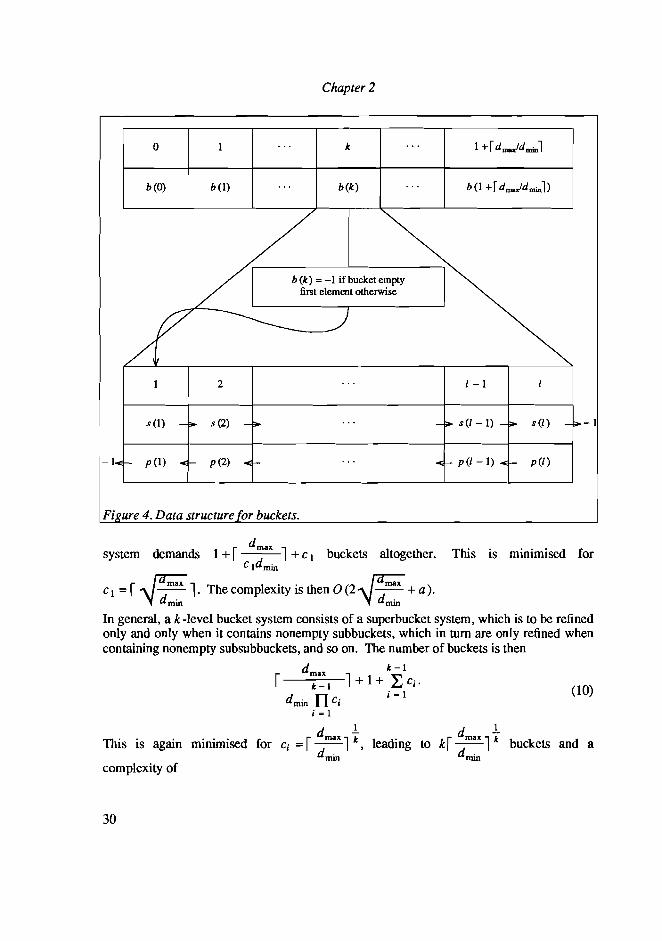
bucket i = L~ ~) J The bucket itself has the structure of a linked list To maintain ffiln

d buckets a system of three pointers must be introduced b (i) (i =0 1 + r~1) is an

d min

arbitrary node of bucket i not necessarily the minimum travel time node b (i) =-1 if bucket i contains no elements sU) U = 1 n) is the next node in the same bucket p U) is the preceding node in the bucket s and p = -1 if there are no such nodes Initially all buckets are empty only the zero-th bucket contains the source node s The shortest path tree algorithm thus becomes

Algorithm BUCKET 1 Initialisation

for allj E N - Is tt(j) = 00

28


precO) =j pO) = sOl =-1

r dax 1for all k E OI2 bullbullbull 1 + drn

b(k) =-1 for j =s

tt(j) =0 precOl =s b(O) =s

2 Selection and updating find lowest non-empty bucket b(k) F-l for each i E b(k)

for each j E FS(i) with tt(i) + dij lt ttOl tt(j) =tt(i) + dij prec(j) =i change bps accordingly

empty b(k) 3 Iteration

if all buckets are empty stop else goto 2

In cases where the network (G D) is not completely connected so that some connections have infinite weights the above definition of d max has to be modified As the union of all buckets has to include all permanent travel times d max must be defined as an upper bound for the travel times at the end of the algorithm A safe bound is dmax = (n - 1) max djj

(jj)e A

because a shortest path will never contain more than n - 1 connections Only when a node gets a temporary travel time less than d max it is put in a bucket

After this the SPT-algorithm with buckets has computational complexity

r dmax 1 r d max 1cc = O(a + 1+ -- ) = O(max(al + -d- )) (9)dmm mill

because n nodes are considered but only when there are more buckets than nodes d d

0(1 +r~1) operations are needed The memory space required is a r~l-vector to dmill dmill

list the buckets and four n -vectors for tt (n) prec (n) p (n) and s (n) Buckets are especially fit for the case where all d jj are integers see Dial et al (1979) only Denardo and Fox (1979) generalise to noninteger djjs

sect37 Bucket nesting

Denardo and Fox (1979) show that the complexity bound can be reduced by introducing a dmax

hierarchy of buckets A two-level system consists of an array of 1 +r d 1 Cl mill

superbuckets with width c Idmill where c 1 is an integer greater than one and a virtual array of buckets with width dmm Only when a superbucket contains nonempty buckets the virtual array is made a concrete array of c 1 buckets to be scanned Such a two-level bucket

29

Chapter 2

0 1 000 Ie 000 1 +f dDWtldminl

b(O) b(I) b(Ie) b(I +f dmaJdminl)

b (Ie) =-1 if bucket empty first element otherwise

~

2 1 -1

0shy s(l-I)shy

- p (I - 1)

11

0 0- s(l) -5 -1s(l) shy 0- s(2) shy 0- shy

- p(l)-1-Er- p (1) -E - p(2) -E -

Fi ure 4 Data structure or buckets

dmax system demands I + r-d--1+ c 1 buckets altogether This is minimised for

CI min

CI = r~ 1 The complexity is then O(2~ + a)

In general a k -level bucket system consists of a superbucket system which is to be refined only and only when it contains nonempty subbuckets which in tum are only refined when containing nonempty subsubbuckets and so on The number of buckets is then

d k-I maxr A -I

d nmin Cj

1+ 1+ L Cj j =1 (10)

j = 1

This is again minimised for Cj = r ddm~x 1t leading mm

to kr dmax 1t buckets

dmin

and a

complexity of

30


13 14 15 16

Fi ure 5 A 4-level bucket hierarch with 256 virtual and 16 concrete arra elements

d max 1+o(max(m kr ~ raquo (11) mm

Finally this is minimised for k = clog[ d dm~x 1 It should be remarked that even with this

mm sophistication the use of buckets may cause problems because the computation time is still

d dependent on dm~x which can be very large as in seismic models with a large range of

mm slownesses

sect38 Combination ofbuckets and heaps

One way to combine buckets and heaps is to order the elements of each bucket in a heap However this is useless because the elements do not need any ordering due to the theorem in sect36 The other way is to keep up a heap containing nonempty buckets This is done by Hansen (1980) who obtains a complexity of 0 (a Clogdmax) Karlsson and Poblete (1983) reach a complexity of 0 (a Clog clogdmax) by utilising the data structure provided by van Emde Boas Kaas and Zijlstra (1977) They recommend their method for the case when d max =0 (n) and refer to the use of simple heaps in other cases

31

Chapler 2

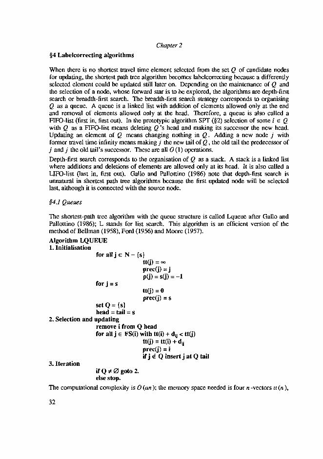
sect4 Labelcorrecting algorithms

When there is no shortest travel time element selected from the set Q of candidate nodes for updating the shortest path tree algorithm becomes Iabelcorrecting because a differently selected element could be updated still later on Depending on the maintenance of Q and the selection of a node whose forward star is to be explored the algorithms are depth-first search or breadth-first search The breadth-first search strategy corresponds to organising Q as a queue A queue is a linked list with addition of elements allowed only at the end and removal of elements allowed only at the head Therefore a queue is also called a FIFO-list (first in first out) In the prototypic algorithm SPT (sect2) selection of some i E Q with Q as a FIFO-list means deleting Qs head and making its successor the new head Updating an element of Q means changing nothing in Q Adding a new node j with former travel time infinity means making j the new tail of Q the old tail the predecessor of j and j the old tails successor These are all 0 (1) operations

Depth-first search corresponds to the organisation of Q as a stack A stack is a linked list where additions and deletions of elements are allowed only at its head It is also called a LIFO-list (last in first out) Gallo and Pallottino (1986) note that depth-first search is unnatural in shortest path tree algorithms because the first updated node will be selected last although it is connected with the source node

sect41 Queues

The shortest-path tree algorithm with the queue structure is called Lqueue after Gallo and Pallottino (1986) L stands for list search This algorithm is an efficient version of the method of Bellman (1958) Ford (1956) and Moore (1957)

Algorithm LQUEUE 1 Initialisation

for aIlj E N - s tta) =00

precU) =j pU) = su) =-1

for j = s ttU) = 0 prec(j) = S

set Q = s bead = tail = s

2 Selection and updating remove i from Q head for all j E FS(i) with tt(i) + dij lt ttU)

tt(j) = tt(i) + dij prec(j) = i if j fi Q insert j at Q tail

3 Iteration if Q lZl goto 2 else stop

The computational complexity is 0 (an) the memory space needed is four n -vectors tt (n )

32


prec (n) s (n) p (n) Although the complexity is 0 (an) =0 (mn 2) which is comparable to DijkSlras complexity this is only a worst-case complexity It appears that Lqueue runs almost 0 (n) in practice This efficiency is based on the nature of breadth-first searching the search is organised in a way which resembles concentric waves Iravelling away from the source node

sect42 Double-ended queues

A double-ended queue or deque is a mixture of a stack and a queue At the first insertion of a node into Q Q is viewed as a queue so the insertion occurs at the tail of Q At later updatings the node is inserted at the head so Q is viewed as a stack The reason for this Ireatrnent is that at each time a node j with Iravel time tt U) is updated except the first time when it is updated from infinity all nodes behind it in the current Iree should also be updated This way their tum will come soon

DEsopo and Pape (pape 1974) applied the deque slructure in their algorithm Ldeque

Algorithm LDEQUE 1 Initialisation

for alIj E N - is ttG) =00

prec(j) =j p(j) = s(j) = -1

for j = s tt(j) = 0 prec(j) = s

setQ = is] head = tail = s

2 Selection and updating remove i from Q head for all j E FS(i) with tt(i) + dij lt tt(j)

if j Ii Q then if tt(j) = 00 insert j at tail Q else at head Q

tt(j) = tt(i) + dij prec(j) = i

3 Iteration if Q f= 12 goto 2 else stop

The computational complexity is in its worst case 0 (n 2) but when the network is sparse (a = 0 (nraquo and almost planar (mappable on the IR2 without intersection of arcs) the practical complexity is 0 (n) In fact Gallo and Pallottino (1986) state that Ldeque apart from the risk of being in a worst case is the most efficient shortest path algorithm for sparse graphs To avoid risks other variants like Lqueue can be used

33

Chapter 2

sectS An empirical comparison of DUKSTRA HEAP LQUEUE and LDEQUE

The computation time of the DUKSlRA HEAP LQUEUE and LDEQUE-algorithms to construct the shortest path tree of one source node are measured in the following experiment with regards to the application on seismic ray tracing The type of networks used is as in Figure 6 These are characterised by nJlt cells in x -direction nz cells in zshydirection n nodes on every cell boundary and consequently

(12)

nodes in all A forward star contains 6n nodes in the inner network 3n on its boundaries The number of finite arcs is a = 6nnJlt nz bull The weights are Euclidian distances The relation between computational complexity and number of nodes is investigated for each algorithm with n constant and nJlt = nz increasing one by one from 1 to 100 This means that each forward star in the whole experiment contains the same number of nodes and a =O(n)

The results are plotted in Figures 7 and 8 Through each series of data points a parabola is drawn regardless of their real asymptotic relation which is after all not exactly known

Conclusion

The type of network to represent a seismic velocity field is characterised by extreme sparseness (a ~ lOOn mostly) arbitrarily large sizes (n raquo 103

) arbitrarily large ranges of weights but scarcely any planarity According to these qualities the shortest path algorithms can be judged Doing this one must make a distinction between the theoretical complexity and the practical complexity

Algorithm Dijkstra without list appears to have a strictly quadratically asymptotic

network used or test on com utational com lexi

34


o o

~ I)

al ~ ell 0 EO_ 0

~ o iii 0 051) E 8

o

DIJKSTRA

OTHERS shy

o 20000 40000 number of nodes

Figure 7 Computation time offour shortest path tree algorithms as a function of the number 0 nodes

0 8 ell

~ ell E

8c

0 ltll) 5 C E 8

Figure 8 Blow-up ofFigure 7

D JKSTRA E


complexity just as can be foretold by the theoretical bound Algorithm Dijkstra-list is slightly better but still not better than quadratic The application of heaps causes a strong reduction in computation time 0 (n 210gn ) in theory but indistinguishable from 0 (n) in practice In the present case this cannot be improved by ~-heaps or F-heaps The 0 (a) bound is reached theoretically by labelsetting algorithms with buckets

Labelcorrecting algorithms are characterised by large theoretical bounds (Lqueue 0 (an) Ldeque 0 (n 2)) but with reasonable bounds in practice This reasonability however depends strongly on the sparseness and planarity of the network which is disadvantageous for the application under study Figure 8 shows that Dijkstra with heaps outperfonns the labelcorrecting algorithms Therefore Heap or one of its improvements should be pointed out as the fastest algorithm in the present network type It has a secure theoretical bound and often an even better practical bound

The question whether the use of buckets or bucket nesting should be preferred to heaps leads to the consideration of the memory space needed In spite of the reductions in storage requirement indicated in sect36 and sect37 the dependence on the range of weights and thus on the regularity of the seismic velocity field causes an undesired inflexibility One could wish to be able to introduce arbitrarily strange or complex models to the ray tracing algorithm but the use of buckets can imply either a large memory space needed or even a long computation time

In this way the Dijkstra algorithm with the application of simple heaps can be preferred to all other algorithms because of 1 a theoretical computational complexity of 0 (n 210gn ) 2 a storage requirement of 4n places 3 its flexibility with respect to its input model

35

Chapter 2

36

Reflection seismology

CHAPTER 3

Reflection seismology using constrained shortest paths

Introduction

Seismic ray tracing with shortest travel time paths in networks is restricted in that only the absolutely shortest paths are found These unconditioned shortest paths always represent the first arrivals on a seismogram like direct refracted or diffracted waves Later arrivals like reflections and multiples caused by discontinuities in the spatial velocity distribution do not travel along the shortest path between a source and a receiver and can therefore not be calculated by a shortest path algorithm This is easily explained by observing that the shortest path is shorter than or equal to a shortest path satisfying some constraint the constraint to visit at least one node of a specified set of nodes Yet later arrivals are of great scientific and economic importance because they contain additional information on the Earths structure

In this chapter a method is developed to circumvent this difficulty It is demonstrated that constrained shortest paths are good approximations of reflections and multiples The conclusion is that each reflection needs one additional execution of the shortest path tree algorithm The constrained shortest paths from the source node or nodes to all other nodes of the network are then calculated This is done with the same efficiency as the calculation of shortest paths The generalisation of the Dijkstra algorithm needed to solve the constrained shortest path tree problem enables the solution of a much wider class of problems the simulation of a so called exploding reflector the calculation of earthquake locations and the migration of zero and nonzero offset data

The first sections sectI sect2 and sect3 are preparations to obtain a graph wherein interfaces and interval velocity distributions can be chosen freely and sets of nodes can be pointed out to reflect shortest paths The constrained shortest path tree problem is presented in sect4 The solution is used in section sect5 to calculate later arrivals Section sect6 gives the physical and mathematical meaning of constrained shortest paths The last sections show some other applications of the generalised shortest path procedure

All examples are given in two dimensions the extension to three dimensions is straightforward

sect1 Definitions and notations

The general notations and definitions used are the same as in Chapter 2 Additional notations used in this chapter are

SeN the source node set is the set of nodes for which tentative travel times are specified before the execution of the Dijkstra algorithm

The nodes are positioned in a rectangular two dimensional grid with nr nodes in the xshydirection and nz nodes in the z -direction and grid units Ox and Bz The grid covers a region of [0100] x [0100] dimensionless distance units in all examples of this chapter Each node is connected with all nodes in a [-55] x [-55J-neighbourhood of it except when three nodes are aligned like for instance (00) (21) and (42) (Figure 1) Such a

37

Chapter 3

~

-

Figure 1 A 20 x 20 grid with forward stars Figure 2 A model of interfaces The black orfourdqrerentnode~ circles are the Beta-spline support points

the small points are the nodes of the network

network organisation allows for a simple definition of a discontinuity namely a curved line separating the nodes into two different geological layers The weight of a connection between two nodes i and j dij which is equal to the seismic travel time from i to j is calculated as

(1)

where the integral is taken along a straight line between i and j and evaluated numerically (see Chapter 6 A practical comparison of the shortest path method with other methods)

The interfaces are constructed with Beta-splines (Barsky 1988) and are determined by 1 support points V where i = Onsupp denotes the indices of the points 2 a Beta-spline curve consisting of nsupp continuously differentiable (C 1) segmentsit (u) where i = 0 nsupp and 0 ~ u ~ 1 for each segment 3 two parameters ~l and ~2 that determine the shape of the Beta-spline curve These notations can be extended to three dimensions The number of interfaces is neither specified nor limited

nc(i) i = 1 bulln is the colour of node i specifying the layer it belongs to

When later arrivals are computed tt(1i) is the travel time of the first arrival tt(2i) of the second and so on prec (1i) is the preceding node on the shortest path segment prec (2i) is the preceding node on the constrained shortest path segment

38


sect2 The construction of interfaces

In the most general case it is desirable to construct velocity models consisting of continuous layers separated by arbitrarily curved interfaces indicating discontinuous transitions from one layer to another This can be formulated as a set of functions c =ci (x z) when (xz) E layer (i) where i runs over the nwnber of layers and a set of conditions (x z) E layer (i) if Ii (x z) gt 0 (Gjoystdal Reinhardsen and Astebol 1985) A flexible method to construct smooth curves that have the shape of the desired interfaces is modeling with Beta-splines (Barsky1988) (see Appendix A of Chapter 5 Ray bending revisited) An interface is then defined by nsupp+l support points V Vo and V arensupp

the endpoints that are interpolated One interface can only separate two distinct layers so in the case of an interface ending on another interface in point iT three interfaces must be formed each ending in iT (Figure 2) The tangents to the interfaces in iT can be fixed by vicinal points

sect3 Separation of nodes by interfaces

Despite the flexibility of Beta-splines for the construction of interfaces they provide an explicit parametric form for their shape This means that points of the interfaces can be generated easily but that an arbitrary node of the network cannot be oriented with respect to the interfaces Therefore an array of indices is constructed that refer to the layer to which the node belongs This is done by colouring the nodes First the nodes adjacent to the interfaces are coloured by a so called painti~ algorithm (Newman and Sproull 1981) For each calculated point of the Beta-spline Qi (u) the nodes concerned can be found by truncating (1 (u) to the grid size

v v+ (BxO) (2)v+ (O8z) v+ (Bx 8z )

where

It =(L Qi(~~(U) JBx LQi~(U) J Bz ) (3)

These four nodes are the nodes coated by the brush at (1 (u) Then for each such node it is determined at what side of the interface it lies A criterion for this is

F =det~- (1(u) d~ (U)] (4)

where r denotes the position of one of the brushed nodes and del denotes the determinant

of the 2 x 2 matrix with colwnns r - (1 (u) and d(1 (u) the tangent vector at (1 (u) ~ du

dQmiddot When F =0 r - (1 (u) and du (u) are linearly dependent and the node lies on the

tangent When F gt 0 it lies at the left side of the tangent when F lt 0 it lies at the right side (Figure 3) The four nodes of the brush can then be coloured with the colours of the layer left to the interface or right to the interface

After treating all interfaces in this way the nodes adjacent to them are painted To fill in

39

bull bull bull bull bull

Chapter 3

o 0 000

tangentF = 0 coloured nodes

e bullbull bull bull 000~ o 0 000

Beta-spline (l (u)

the regions between them the following loop can be executed

1 For each node i from 1 to n look whether it is coloured If this is not the case consider its four neighbours j If one is coloured give i the same colour 2 Repeat l for each node from n to l

The idea behind this procedure is that when all nodes neighbouring interfaces are painted each layer is surrounded by a closed chain of nodes with its colour The neighbours of uncoloured nodes all have the same colour if any An additional check must be done at the triple points of interfaces because the nodes in their neighbourhood may have been coloured more than once

sect4 The constrained shortest path tree problem

The general constrained shortest path tree problem is the problem to find the shortest paths between pairs of nodes satisfying some constraint The constraint poses a restriction to the paths available for searching a shortest one The constrained shortest path is often longer than the unconstrained shortest path equality occurs only when the shortest path happens to satisfy the constraint

There are different types of constraints For example the paths can be forced to visit all nodes of a subset of the graph An extreme case of this is the traveling salesman problem the problem to find the shortest path from one node to another visiting all other nodes of the graph Also the paths can be forced to visit the nodes of the subset in a predescribed order One could also fix only the number of nodes to be visited on the way differing from each other or not The problem to determine the shortest path not equal to the already known one is the second shortest path problem For a survey on these problems see for instance the bibliography of Gallo et al (1982)

The constrained shortest path tree problem referred to here is the problem to find the shortest paths from one node to all nodes each path visiting at least one node of subset of the graph (Figure 4) The solution to this problem proposed here is based on a generalisation of the initialisation step of the Dijkstra algorithm As is explained in Chapter I the Dijkstra algorithm divides the set of nodes N into a set of permanently labeled nodes P and a set of temporarily labeled nodes Q P contains nodes with known travel times along shortest paths from the source node Q contains nodes with tentative travel times Initially only the source nodes travel time is known (tt(s) = 0) and all other travel times

40


Figure 4 The constrained shortest path problem given a graph G a source node s and a subset S c G nd the shortest aths rom s via S to all nodes i

are unknown and are thus set equal to infinity Then an iterative procedure is started In each iteration all nodes j in Q connected with nodes i in P are updated according to the rule

ttU) = min(tt U)tt(i) + dij ) (5)

The minimum travel time node in Q is then transferred to P and the next iteration is done The procedure ceases when Q is empty because then the travel times to all nodes in the graph are known

The purpose of the generalisation is to predestinate the set Q before executing themiddot algorithm Instead of initiating all travel times with infinity one can initiate a specified node set with finite travel times As there is no longer a unique source node this set will be called the source node set S The shortest path algorithm is then

Algorithm DIJKSTRA-GENERALISED 1 Initialisation

for aUj EN - S tt(j) = 00

prec(j) =j for j = S

tt(j) is specified a priori prec(j) =j


find i E Q such that tt(i) = min tt(j)Je Q

for all j E FS(i) with j E Q and tt(i) + dlj lt tt(j) tt(j) =tt(i) + dij prec(j) = i

Q = Q- [i] 3 Iteration

if Q j 0 goto 2 else stop

Note that step 2 and 3 are identical to the original Dijkstra-algorithm Note also that when

41

Chapter 3

S is organised as a linked list or as a heap the respective Oijkstra algorithms are generalised in the same way so the efficient algorithm Oijkstra with heaps can be used again

Whether or not the travel times in S will change during the rest of the procedure depends on their range and distribution If all finite initial travel times are equal to each other they will no longer be updated so all nodes in S act as coupled sources also called a centroid (000 and Pang 1984) On the other hand if the initial travel times differ from each other the node with a minimal travel time acts as a pseudo source When in presence of such a pseudo source the travel times along shortest paths from the pseudo source to other nodes in S are greater than their predestinated travel times the other nodes act as retarded sources In the other case when the travel times of the other nodes are greater than or equal to the travel times along the shortest paths to the pseudo source it is just a real point source

Full use of this idea of coupled source nodes will be made in the following sections The application of it on the constrained shortest path problem is as follows First the original unconstrained shortest path tree problem with s as source is solved the result is tt (li) and prec (li) i = 1 n The nodes of subset S that must be visited by the constrained paths are then selected and their travel times eventually ordered in a heap The travel times of the other nodes are reset to infinity The nodes of S are then used as a source node set and the algorithm is executed for a second time the result is tt(2i) and prec (2i) i = 1bullbull n This solves the problem of finding the travel times of all nodes of N of shortest paths from s via S The paths themselves are obtained as a composition of the shortest paths of the first and second run of the algorithm which are stored in the arrays prec (1n) and prec (2n)

For a proof of correcbless of this procedure consider the network (G 0) with an extra node S2 connected with all nodes j of S and with no other nodes (Figure 5) The weights dsj j E S are equal to the travel time along the shortest paths from s I to j For the other nodes and connections (G 0) =(GD) Then find the shortest paths from s2 to all nodes

the constrained shortest

42


i EN This procedure is the same as the one outlined above after the first iteration all nodes j of S are updated with tt U) = dsj and then S is used as a source set for the rest of the graph The result is certainly a shortest path tree from S2 with all paths visiting S

Consider Figure 6 to see how the algorithm works A simple network (G JJ) is drawn consisting of 7 nodes 2 on the Earths surface and 5 on an interface (n bull n7) The velocity in the first layer is 10 The distances are Euclidian distances with d7 = 20 and d =10 and the rest following from Pythagoras rule As a consequence of the triangle inequality the unconstrained shortest paths from n to the other nodes follow the direct connections Thus

tt(lnz) = 10prec(Inz) =n

tt(In3) =1OZ+052 112prec(ln3) =n

tt(ln4) =1OZ+ IOZ 14Iprec(In4) =n

tt (ln 5) = 1OZ + 152 180 prec (ln 5) = n

tt(ln~ = 1OZ+ 2OZ 224prec(In6) = n

(6)

The shortest paths from n satisfying the constraint to visit the set S = n2 n3 n4 n5 n6 are now calculated by setting tt (2n ) =tt (2n 7) =00 and tt (2n =tt (ln for j E S The generalised shortest path algorithm is run with the times tt(2i) as input The nodes of set S will no longer be updated because tt (2n lt tt (2i) + dij for all j E S and i EN so tt (2n = tt (ln and prec (2j) =j n can be updated namely

tt (2n ) = Jlins(tt (2n + dJ) = tt (2n z) + d =2 X d =20 (7)IE

20 )lt

S

n7 Earths surface

interface

Ie network

43

Chapter 3

and prec (2n I) = n 2 The same applies for n7

tt(2n7) =min(tt(2j) + dj) = j e S

min(100 + 224 112 + 180 141 + 141 180 + 112224 + 1(0) =

= 2 x 141 = 282 (8)

and therefore prec(2n7) =n4 tt(2n l ) and tt(2n7) cannot be decreased any more so the process is finished The travel times along the constrained shortest paths are known at this moment tt(2i) The paths themselves are obtained as prec (2i) i E N and then prec(1j) jESSO (nln2nl) (n2n2n1) (n 3n3nl) (n4 n4 n l) (nSnSnl) (n6 n6 n I) and (n7 n4 n I) The last one is the desired reflected ray path from n 1 to n7

44


sect5 The calculation of later arrivals

With the preparations of the previous sections it is now possible to calculate later arrivals on the seismogram After the shortest paths have been found one can indicate manually or otherwise a set of nodes to scatter the received rays In particular one can point out a set of nodes with colour nc (i) =nr each having a neighbour with colour nc(i) =nl When these nodes are used as a source node set the shortest paths via the interface separating the layers numbered nl and nr are found Additionally one can point out another set of nodes to scatter again the scattered wave field It can thus be concluded that the calculation of each new phase or event in the seismogram requires an extra run of the Dijkstra algorithm

Consider for example the model of Figure 2 The grid consists of a grid of 50 x 50 nodes and is divided in 5 homogeneous layers with velocities c (I) = 10 c (2) = 15 c (3) = 20 c (4) =25 and c (5) =30 One surface node is chosen as a source and the shortest paths are computed This is shown in Figure 7 The nodes just below the interface between layers 2 and 3 are selected and chosen to reflect the shortest paths Note that the interface constructed by means of Beta-spline curves is discretised on the grid so that it is no longer smoothly curved The result is shown in Figure 8 Reflected ray paths are visible in the layers I and 2 transmitted ray paths in the layers 3 4 and 5 and critically refracted rays at

45

Chapter 3

the interface between layers 2 and 5 Note that the transmitted ray paths are exactly equal to the direct rays in Figure 7 This is a manifestation of the fact that shortest paths that accidentally satisfy a constraint are equal to constrained shortest paths A second reflection is shown in Figure 9 The reflected ray paths from Figure 8 are ordered to reflect again at the interface between layer 1 and 2 Reflections and transmissions can be seen The latter are again exactly equal to the ray paths in Figure 8

sect6 Physical significance of constrained shortest paths

A careful contemplation is needed when looking at the constrained shortest paths and trying to classify them as a known physical phenomenon

The physical meaning of unconstrained shortest paths can be based on Fermats principle in the original formulation as a minimum time principle The shortest path between two points is a path along which the seismic energy propagates in the high frequency limit If it has a nonnegligible amplitude it corresponds to the first observed arrival at the receiver The first arrivals can be direct waves refractions or diffractions Reflected rays are not generally represented by shortest paths because usually there is a better candidate with a shorter travel time than the reflected ray path

46


Generally constrained shortest paths are not minimum time paths but consist of segments that are themselves shortest paths between their end points Therefore Huygens principle can be used to justify the physical meaning of the constrained shortest path The first segment has the meaning of a minimum travel time path from the source to the reflection point According to Huygens principle this point then acts as a secondary source from where the second segment departs The second segment is again a minimum travel time path between the reflection point and the receiver (or the next reflection point)

It is however not yet clear if the selected points form a real scatterer that is if its backscattering coefficient is nonzero and the scattered waves interfere constructively If it is not a physical scatterer the constrained shortest path may still obey Huygens and Fermats principles but there is no real seismic energy traveling along it Therefore one should use the foreknowledge that nodes with a velocity different from the velocity at one or more of its neighbours scatter received energy Such nodes can be selected for instance by taking all nodes of one layer facing another layer The nodes then simulate an interface This procedure was followed in section sect5 More generally one can choose single points or sets of points and specify that they should scatter energy The shortest path method then finds along which trajectory and at what time the seismic energy travels but it does not tell whether the energy is real or phantom

A restriction to the constrained shortest path method is that when a shortest path already satisfies some constraint the constrained shortest path does not differ from it This means that supercritically reflected waves cannot be found as they are preceded by refracted waves which satisfy the same constraint to visit an interface Also triplications in the travel time curve caused by strongly curved interfaces cannot be found unless the interface is split up into smaller parts each one to be investigated in tum

Fi ure 10

47

Chapter 3

sect7 Exploding reflectors

In the migration of zero-offset data the exploding reflector model plays an important role In zero-offset data the source and receiver location are supposed to coincide The ray paths to and from the interface then coincide also In addition they intercept the interface at right angles to strike Therefore it can be assumed that zero-offset data are caused by virtual explosions at the reflectors the travel times multiplied by two

It is evident that this situation can be simulated by setting the travel times of all nodes at the interface to zero and then running the shortest path algorithm As a pleasant circumstance there is no restriction to homogeneity of the medium between the interface and the receiver it could contain other interfaces as well However multiple reflections are not well described by the exploding reflector model

Figure 10 shows a model of three layers I 2 and 3 with velocities 10 15 and 20 In Figure 11 the explosion of the first layer is shown calculated with the generalised version of the Dijkstra algorithm

48

Reflection seisrrwlogy

sect8 Migration

A common problem in exploration seismics is migration to reconstruct the positions of the interfaces from reflection travel times and interval velocities The idea of coupled source nodes can be helpful to do this simultaneously for all measurements The migration of zero-offset data is the simplest case

sect81 Migration of zero-offset data

It is supposed that only zero-offset data at the Earths surface and interval velocities are given and that the model of interfaces is unknown The task is to find the real geometry of the interfaces by migrating the surface travel time data When these are divided by 2 they are exactly the travel times obtained by the exploding reflector model These can be backpropagated in time the wavefront at time zero is then equal to the interface The backpropagation can be done by multiplying all travel times with -1 and then running the shortest path procedure Yet the procedure only works when the model is known This means that at first the shortest zero-offset travel times must be migrated through a medium with the uppermost interval velocity (distribution) everywhere The other interfaces can then be reconstructed in an iterative process

Zero offset travel times were computed for the model of Figure 10 and plotted in Figure 12 The task is now to reconstruct Figure 10 with Figure 12 and the knowledge about the interval velocities 10 15 and 20 With the shortest path method this can be done in two steps

First the one-way travel times of the first reflection are multiplied by -1 All surface nodes are used as source nodes with these travel times as input to the shortest path algorithm that is executed in a medium with a constant velocity 10 From its output the wavefront at time ois considered to be the first interface Secondly the travel times of the second reflection are treated in the same way They are backpropagated in a medium with one already

~

I I-shy I I - I -

0

CD O ~

E co

+==0 0 -0 Ishy~L() lttl ~o - 0 Ishy

ltt --

-

-

~ -I I I I I

o 250 500 750 1000 distance

FiRure 12 Zero offset travel times for the model in FiRure 10

49

-----

------------

------------------

-----

Chapter 3

-----r ---------~---

-_---~-----2 - -_-_-_--=-----c~

~-----

---~-3

Figure 13 Backpropagatedfieldsjrom Figure 12 Broken lines model of Figure 10 Thin solid lines isochrons Heav solid line isochron at time O

known interface and two interval velocities 10 and 15 The two backpropagated fields are shown in Figure 13 with thin lines the wavefronts at zero time with heavy lines The real interfaces from Figure 10 are plotted as well (dashed lines)

sect82 Migration ofnon-zero offset data

A little more complicated is the case where source and receiver occupy different positions Consider for instance the common shot point geometry one source and many receivers The ray paths and travel times along them to and from the interfaces are no longer equal

Suppose that the interval velocities and the reflected travel times are known To reconstruct the uppennost interface the shortest paths from the source node and the

50


backpropagation of the reflected travel times must be found in a medium with the uppennost interval velocity everywhere The backpropagation is again done by multiplying all travel times by -1 and running the shortest path procedure The positions where the direct travel times and the backpropagated times sum up to zero coincide then with the first interface The other interfaces can be again reconstructed in an iterative process Thus the migration of each interface demands two runs of the shortest path algorithm

These ideas are illustrated with the example of sect8l only the first interface is reconstructed The primary and reflected fields are shown in Figure 14 The backpropagation of the reflected field as measured at the Earths surface is shown in Figure 15 (left) The backpropagated reflected field and the primary field summed up are

~ ======--gt

Figure 15 Backpropagatedfieldfrom travel times of Figure 14 (left) and superposition of primary and backpropagated field (right) Broken lines model of Figure 10 Thin solid lines isochrons Heav solid line isochron at time O

---shy

Fi ure 16 Primar

51

Chapter 3

given in the same Figure right The thin lines are the summed up wavefronts at nonzero times the heavy line is the wavefront at zero time the dashed line is the actual interface to be reconstructed An uplifting of the calculated interface visible at the right side is due to incomplete data sets some reflections do not reach the surface

Another illustration isolates this uplifting or smiling In Figure 16 the primary field (left) is scattered by one diffraction point (right) The backpropagated field (Figure 17 left) now consists of three parts the upper triangle contains relevant infonnation and the two regions next to it contain circular wavefronts from both ends of the receiver line The superposition of the primary field and the backpropagated diffracted field (Figure 17 right) has a sharp edge ending in the diffraction point The heavy line again represents the summed up wavefronts at time zero The effect of choosing a wrong interval velocity to propagate back is demonstrated in Figure 18

sect9 Earthquake location

The idea of coupled source nodes has another application which is not in the direct context of reflection seismology namely source location in a known medium from first arrival times A well known example is earthquake location The situation is then slightly different from the previous section the velocity model and a sufficient number of first arrival times from an earthquake to the Earths surface are known but the earthquake location and its origin time are unknown and to be found The number of observations must match at least the number of unknowns (the x and y -coordinate and the origin time of the event and sometimes the depth coordinate z) but preferably the problem is fonnulated as a robust least squares problem by having much more than four observed arrival times Chapter 7 gives a detailed description of earthquake location by means of the shortest path method based on least squares minimisation and supplemented with a complete error analysis

In this section only a very simple two dimensional example is given Figure 19 (left) shows

Fi

52


the shortest paths from a subsurface source in the linear velocity field c (x z) = 10 + 001z The problem is now to reconstruct the source position and the origin time from the first arrival times at the Earths surface and the known velocity model Again backpropagation of the travel time measurements is the solution Three of them are multiplied by -1 and used as source times for the proper nodes As a result the medium is separated by the shortest path algorithm into sections each one being reached first by a source node and each one ending in the earthquake location (Figure 19 right) Thus the earthquake position is found by the intersection of the separations of these sections The corresponding origin time is obtained by subtracting the travel time from the source to one of the receivers from its first arrival time

Fi ure 19 Earth uake location

53

Chapter 3

Conclusion

The constrained shortest path algorithm can be used to calculate later arrivals in the seismogram These later arrivals should be interpreted as energy scattered by a specified set of nodes thus determining their physical meaning The algorithm is based on a generalisation of the Dijkstra algorithm which predestinates the travel times of chosen nodes This generalisation allows fitting together single source nodes to more complicated sources As a byproduct other experiments can be carried out like migration or the exploding of a reflector

The question of the accuracy of the found results has not been treated here because the travel times of the constrained shortest paths are as precise as the times of the shortest paths they consist of Finally the computation of a scattered wave requires the same amount of time as computing shortest paths

54

Accuracy

CHAPTER 4

Accuracy of ray tracing by means of the shortest pathmethod

Introduction

The discretisation of a seismic velocity model into a network introduces errors in the ray geometry and the travel time along the rays because of the finite number of possible paths and travel times It can be expected that these errors depend on the characteristic elements of the discretisation

First there is the sampling of the velocity field by a finite number of nodes Whether the sampling is sufficient depends on the variations in the velocity field the spatial density of nodes and the definition of the weights of the arcs The travel time along a shortest path is defined as the sum of the weights of the connections it consists of therefore the travel time error is directly dependent on the sampling of the model

The structure of the network itself also influences the accuracy of the ray paths and the travel times Ray paths are generally smooth curves but the shortest paths are polygonal As they can follow only preference directions a kind of numerical anisotropy is introduced by the network

To be able to rely on the results of the shortest path calculation it is necessary to estimate these errors as a function of parameters controlling the network density and structure The estimated accuracy must then be compared with the computation time which is dependent on the same parameters Both the accuracy and the efficiency determine the feasibility of the shortest path calculations in relation to the desired result which is for instance the shortest paths from one source point to the entire volume the shortest paths to points in shadow zones or the shortest path between only one source receiver pair

In this chapter rules are formulated that predict the travel time and ray path errors as functions of network parameters In the first section both notations and the network types used to test the rules are introduced sect2 shows that part of the error is caused by the nonuniqueness of shortest paths In sect3 an asymptotical relationship is established between the travel time error and two network parameters This relationship is tested in sect4 sect5 gives some alternative methods for the improvement of calculated travel times and ray paths in case they are too inaccurateshy

Only two dimensional examples are used the extension to three dimensions is straightforward

sect1 Notations and definitions

Apart from the general notations and definitions introduced in Chapter 1 the following are used here

SP (i j) is the shortest path from node i to node j Equivalently SP (r 1j) is the shortest path from a node i at r to a node j at rj SP (ij) is the shortest path in the network (G D) that is the concatenation of nodes SP 0 rj) is its equivalent in the three

55

Chapter 4

dimensional Euclidian space that is a polygonal path with the edges at the node locations

f (i j) or t (r rj) is the travel time along SP (i j) and SP (r rj) respectively This travel time is obtained as the sum of the weights of the segments of the shortest path the weights are the numerically integrated slownesses along the segments

F (r rj) is the minimum travel time path between r and rj a spatial curve that minimises

f ltis among all continuous curves y connecting r and rj Such a path is referred to as a 1 c

Fermat path Existence of a Fermat path is guaranteed by assuming that each nonempty set

of candidate curves yI f ltis ~ M lt oo is compact and f ltis a continuous functional of y J c 1 c

(according to Weierstrap see Funk 1962) This assumption is valid when the velocity c (1) is twice continuously differentiable

T (r rj) is the travel time along the Fermat path F (r rj) T (r rj) is the smallest

possible value of f ltis bull 1 C

The minimum travel time path or Fermat path is used as a mathematical object to which the shortest path calculations are compared In physics the Fermat path is the curve along which the seismic energy propagates in the high frequency limit Therefore it is reasonable to base the error analysis on the Fermat path and the travel time along it

E = f - T is the travel time error It depends on the spatial coordinates r and rj on network- and $rid-related parameters and the velocity field and its derivatives The definitions of T(r rj) T (r rj) F (r rj) SP (r rj) SP (i j) and E are all independent of the source configuration Point sources and coupled sources (see Chapter 3 Reflection seismology using constrained shortest paths) can be treated in the same way

Asymptotic relations used to describe the travel time error as a function of some network related quantities are denoted with Landaus symbols f (x) =0 (g (x)) (x ~ a) means

I flaquoX)) I is bounded for x ~a and f(x)=o(g(x)) (x ~a) means lim flaquoX)) =0 gx ~agx

When a = 0 as is mostly the case (x ~ a) is skipped This is a convention different from Chapter 2

One can use asymptotic relations to formulate Fermats principle let F (11 rj) be a Fermat path pound gt 0 a small parameter and y a disturbance curve that vanishes in the source and receiver points y(l1) =)(rj) =O Both curves are parametrised by a real parameter that increases monotonically along the curve Addition of two curves is understood as the addition of its coordinates at corresponding values of the curve parameter The travel time along the disturbed curve T(F + ey) then obeys the relation

T(F +poundy) =T(F) +0 (pound2) (1)

This means that the travel time error is generally one order of magnitude smaller than the error in the path geometry The altitude of a slowly shelving hill can be measured more exactly than the position of its summit Fortunately in exploration seismology and travel time tomography both applications of seismic ray tracing precise travel times are often more relevant than precise ray paths which are a mere mathematical idealisation whereas in reality a wider area the Fresnel zone influences the travel time In this chapter an accuracy of 01 in the travel time is chosen as a target The ray geometry error then

56

Accuracy

follows with one larger order of magnitude

sect11 Network description

The networks used in this chapter to test the accuracy of shortest path and travel times along them are of the grid type and the cell type

In the grid organisation of the network the nodes are positioned in a rectangular two dimensional spatial grid with ncr nodes in the x direction and n nodes in the z direction the total number of nodes is n = nrnbull The grid is equidistant in each coordinate direction with coordinate ranges [XI xii and [z I zil and grid spacings

ax = (xz - xI)(nr -1) az = (zz - zl)l(n - 1) (2)

Each node can be given real coordinates r = (xz) and discrete coordinates (ir i) ir = O bullnr - 1 and i = 0 n - 1 where

(3)

Each node is connected with all nodes in a [-nsd nsd] x [-nsd nsd]-neighbourhood of it its forward star An example is given in Figure 1 nsd is then the number that determines the size of the forward star the number of connections with one node (number of standard distances distances that are computed and stored in memory before executing the shortest path tree algorithm) is bounded above by 4(nsd + 1)nsd By convention nsd = 0 is not to describe the case in which there are no connections at all but the case in which a node is connected with four adjacent nodes its north south east and west neighbours Such a

~

~

lo Ogt - bull bull -middot middot middot middot middot middotmiddot middot ~ ~ - - middotmiddot middot middot middot middot middot middot

bullbullbullbullbullbullbullbull A bullbull 1

Figure 1 A 20 x 20 grid with the forward Figure 2 A 5 x 5 cell model with 10 nodes stars offour nodes nsd = 2 (left) 4 (above per cell boundary and the forward stars of right) 5 (center) and 7 (above left) three nodes

57

Chapter 4

network will be called the Streets of New York (Figure 3 left) nx and n is used to control the spatial distances allowed nsd is used to control the number of angles allowed The weight dij of a connection between nodes i and j is computed as

jds dij = f~ (4)

where the integral is taken along a straight line between i and j and evaluated numerically The choice for the integration rule has a direct consequence for the accuracy of the computed travel time When dij is computed with the trapezoidal rule

d _1(_1_)11 r -rmiddot11 (5)I) - 2 cmiddot + C ) )

where II 11 is the Euclidian norm the travel time is correct at most up to 0 (ox 2) All grid networks in this chapter use the above definition for the weight of an arc Other more advanced schemes take the variations of the velocity on the nodes between i and j into account (see Chapter 6)

The cell organisation of the network is taken from Nakanishi and Yamaguchi (1986) It is suitable for seismic tomography The two dimensional medium is divided into rectangular cells with a constant velocity the nodes are placed on their boundaries (see Figure 2) Two nodes are only connected with each other when there is no cell boundary between them The cell networks are characterised by nx cells in the x -direction n cells in the z -direction and n nodes per cell boundary The total number of nodes is n = n(nx + n + 2nx n) The parameters nx and n are used to control the spatial distances allowed n is used to control the number of angles allowed The weight djj of a connection between two nodes i and j is defined as the Euclidian length of the connection divided by the velocity of the cell between i and j

sect2 Nonuniqueness of shortest paths

The grid organisation of a network allows for a simple examination of the errors that are introduced by discretising a seismic model into a network

If the shortest path from one node to another in a network representing a homogeneous model would be unique it would be possible to derive a simple error estimation in the ray geometry In a network representing a homogeneous model with velocity equal to unity the weights of the connections are equal to their Euclidian lengths This means that the triangle inequality

(6)

can be used to construct shortest paths Now if the shortest path from i to j SP (i j) is uniquely determined every other path between i and j has a longer travel time This means that the Fermat path which is a straight line in a homogeneous model lies in a close neighbourhood of the shortest path for instance not further away than the closest nonshyshortest path The node spacing is then a measure for the accuracy of the ray geometry For special types of networks such as the grid networks or the cell networks this can be stated precisely with the help of the triangle inequality In the following however it is shown how the nonuniqueness of shortest paths infl uences the accuracy of the path

58

Accuracy

geometry and the travel time

In a homogeneous model covered by a grid network as described in the previous section the number of shortest paths from one source node to another node can be derived with the help of recurrence relations The nodes of the grid are given discrete coordinates

LX-X1J d LZ-Z1J Th cd () (00) dth I = ~ an J = ~ e source is positIon at I J = an e opposite

node has discrete coordinates (n - I nz - I) The number of shortest paths from (00) to (i j) is denoted as p (i j)

The simplest situation is nsd = 0 the Streets of New York (see Figure 3 left) The recurrence relations for p (i j) are

p(i 0) =p (Oj) = 1 (7)

p(i + Ij + 1) =p(i + Ij) + p(i j + 1) (8)

both for i j ~ O These follow from the observation that to reach (i + lj + 1) along shortest paths one should travel via (i j + 1) or (i + Ij) The relations can be solved with the help of a generating function g (xz) == L p (i j)xizi (0 ~ XZ 1) a usual procedure

iJ ~o

from combinatorial theory

g(xz) = L p(ij)xizi iJ ~ 0

=1+ LP(iO)xi + LP(Oj)zi + L p(ij)xizi i~i i~l iJ~1

x z = 1+ -1- + -1- +z LP(ij)xz l +x LP(i j)xz l

-x -z i~1 i~O

j~O i~l

Figure 3 Three networks with 10 x 10 nodes and nsd =0 (the streets of New York left) nsd == 1 (middle and nsd = 2 ri ht

59

Chapter 4 x z =1+ -1- + -1- +z(g(xz)- LP(Oj)ZI)+X(g(xz)- LP(iO)x) -x -z jZO iZO

=1+ (x + Z )g (x z ) (9)

so

g(xz) = 1

l-x-z =

1L (X + z)

1z0

1 k 1= L L ()x z - 1ZOi=01

= L (i iJZ 0

~ I

j)xi zj (10)

Therefore p (i j) =(i ~ I

j) These numbers are arranged as follows

1 1 1 1 1 1 1 1 1 1 1 2 3 4 5 6 7 8 9 10 1 3 6 10 15 21 28 36 45 55 1 4 10 20 35 56 84 120 165 220 1 5 15 35 70 126 210 330 495 715 1 6 21 56 126 252 462 792 1287 2002 1 7 28 84 210 462 924 1716 3003 5005 1 8 36 120 330 792 1716 3432 6435 11440 1 9 45 165 495 1287 3003 6435 12870 24310 1 10 55 220 715 2002 5005 11440 24310 48620

This is Pascals triangle containing binomial coefficients but rotated and scaled into a rectangle The nodes on the sides of the grid can be reached with a unique shortest path the shortest paths to the nodes on the diagonal (i j) i ~ 1 are far from unique

The second case is nsd = 1 (Figure 3 middle) The recurrence relations are

p (i 0) =p (Oi) =p (i i) = 1 (1 I)

for i ~ 0

P (i + 1j + 1) =P(ij + I) +P (ij) (12)

for i gt j ~ 0 and

p(i + lj + 1) = p(i + 1j) +p(i j) (13)

for j gt i ~ O These numbers are arranged as

60

Accuracy

1 1 1 1 1 1 1 1 1 1 1 1 2 3 4 5 6 7 8 9 1 2 1 3 6 10 15 21 28 36 1 3 3 1 4 10 20 35 56 84 1 4 6 4 1 5 15 35 70 126 1 5 10 10 5 1 6 21 56 126 1 6 15 20 15 6 1 7 28 84 1 7 21 35 35 21 7 1 8 36 1 8 28 56 70 56 28 8 1 9 1 9 36 84 126 126 84 36 9 1

This scheme shows two skewed Pascals triangles fitted together Now the nodes on the sides and the diagonal of the grid can be reached with a unique shortest path and a strong nonuniqueness appears at the bisections of the diagonal and the sides

The third case is nsd =2 (Figure 3 right) The recurrence relations are

p (i 0) = p (Oi) = p (i i) = p (2i i) =p (i 2i) = 1 (14)

for i ~ 0

p (i + 2j + 1) = p (i j) + p (i + lj + 1) (15)

for 0 lt j and 2j lt i

p (i + 2j + 1) = P(ij) + p (i + 1j) (16)

forOltjltilt2jand

p (i j) = p Ui) (17)

for 0 lt i lt j because of symmetry along the diagonal These numbers are arranged in this scheme

1 1 1 1 1 1 1 1 1 1 1 1 1 2 3 4 5 6 7 8 1 1 1 2 1 3 6 10 15 21 1 2 2 1 3 3 1 4 10 20 1 3 1 3 1 4 6 4 1 5 1 4 3 3 4 1 5 10 10 5 1 5 6 1 6 5 1 6 15 20 1 6 10 4 4 10 6 1 7 21 1 7 15 10 1 10 15 7 1 8 1 8 21 20 5 5 20 21 8 1

By extrapolation of these calculations to higher values of nsd it can be conjectured that shortest paths are uniquely determined only for nodes on a few straight lines through (00) Between those axes of uniqueness the numbers of possible shortest paths form folded Pascal triangles the numbers on the bisections of the axes are the greatest and they grow exponentially with the distance from (00) Nonuniqueness of shortest paths cannot be avoided in a grid with infinitely many nodes (n = n = 00) but only a finite number ofx z

connections per node (nsd lt 00) With a finite number of nodes one can reduce the

61

Chapter 4

nonuniqueness region by increasing the number of arcs per node

The effect of the nonuniqueness of shortest paths is illustrated in Figures 4 through 8 Figure 4 shows the degenerate case of the shortest paths in the Streets of New York a homogeneous model covered by a 10 x 10 grid network with nsd = 0 so that each node is connected only with four neighbours The shortest paths are then forced to follow the directions 0deg90deg 180deg and 270deg Only ray paths that have a favourable orientation with respect to the network are well approximated The shortest paths from (00) to nodes at the upper and left boundaries of the model are uniquely determined and exactly equal to straight lines the travel times along them are equal to the correct travel times The nonuniqueness is strongest at the diagonal (00) ~ (n - 1 nz - 1) for instance there are 48620 paths from (00) to (99) One could hope that the shortest path from the (00) to (n - 1 nz - 1) would follow the diagonal as closely as possible so that a further refinement of the path with other methods could be made (Chapter 5 Ray bending revisited) It is not predetermined what paths the shortest path tree algorithm will find a number of factors influences the outcome The special choice the algorithm makes depends on the order in which the nodes with tentative travel times are updated (see Chapter 1) which in tum depends on the network size and topology but particularly on the nature of the algorithm Each algorithm labelsetting with heaps or buckets or labelcorrecting with queues stacks or double-ended queues can give other results Even if the shortest path would follow the diagonal as closely as possible the travel time along that staircase-like path deviates with a factor fi This is demonstrated by the fact that the travel time along a path (00) (01) (11) (12) (22) (n - lnz - 1) is exactly the same as the travel time along the path following the lower left corner (00) (Onz - 1) (n - Inz - 1) or the path via the upper right corner (00) (n - 10) (n -Inz -1) by step-by-step unfolding the staircase-like path (see Figure 5) However small 8x is made the error remains a factor fi (Figure 6)

Figure 8 shows the shortest paths from (00) to the boundary of the model in a homogeneous medium covered by a series of grid networks with increasing nsd The set of available angles for each value of nsd is shown in Figure 7 It can be seen that the set of

bull bull bull bull bull bull bull bull bullbull bull bull bull bull bull bull bull bull bull bull bull bull bull bull bull bull bull bull bull bull

bull bull bull bull bull bull bull bull bull bull bull bull bull bull bull bull bull bull bull bull bull

Figure 4 Shortest paths in the streets of Figure 5 Two Nmest poth with the ome I I New York travel time

62

Accuracy

Fi ure 6 Shortest orn = 20 30 40 and 50

shy-

I

~- i shy

i 0 shy-CD i

Ul CD ICDI) (raquov - shyCD

U I 0 CO) - i shy

i I) shy- i

I -- i i i i

5 10 nsd

angles is dense in the interval [0deg90deg] for nsd ~ but not with a unifonn density The00

distribution shows gaps near 0deg and 90deg and smaller gaps near 45deg arctg ~ = 6343497deg

and arctg 2 = 2656505deg The travel time error is maximal in these angle ranges and minimal or zero where the Fennat paths follow exactly the available directions

63

Chapter 4

Figure 8 Shortest paths in a homogeneous medium and grids with nx

Ie t to bottom ri hI) nsd = 0 1 2 34 and 5 = 50 and (from top

The situation in heterogeneous models is more complicated while the nonuniqueness of shortest paths may be reduced IL is however not easy to quantify this reduction Also in other types of networks like the cell networks the nonuniqueness of shortest paths may not be analysed as easily as in the above case In any case the nonuniqueness of shortest paths is a source of errors in the ray paths and the travel times along them even when the weight of each connection is computed correctly

sect3 Asymptotic error analysis

The analysis of sect2 suggests an error analysis in terms of the discretisation in coordinates and the discretisation in angles The error in the ray geometry and in the travel time along the ray as found by the shortest path method depends on the number of nodes in each coordinate direction or the adequacy of the sampling of the velocity field and on the number of connections per node or the number of available angles for the shortest paths In the following sections the discretisation in the angles is denoted by ampp and the discretisation in coordinates by amp The error E = t - Tmiddot can be expanded in a series

E(ampPamp)= L Clijamppiampj = Uoo+ClIOampP+U(nOx + (ampP~O ox~O) (18) iJ ~ 0

It will be shown thaL Uoo = ClIO = Uo = O

64

Accuracy

sect31 Angle diseretisation

The travel time error E = t - Tmiddot caused by the discretisation in the direction space can be examined by taking Ox =0 and ampp gt O This means that the node density is infinite but the number of arcs per node is finite The velocity field is sampled completely but the range of possible directions is limited to 0deg ampp 2ampp 3ampp This situation is mimicked by homogeneous models like the ones described in sect2 In the following it is proved that then E = o (ampp2)

Suppose that a Fermat path F reaches a node A and follows its way to node B under an angle lt1gt The shortest path cannot follow this way because of the angle discretisation The best alternative is the path via the node C (see Figure 9) The following definitions are made D is the orthogonal projection of B on the line AC ltIgt is the angle BAD ampp is the

angle BCD Os is the distance AB The velocity is constant and equal to c OTmiddot = Os is _ c the exact travel time along the Fermat path from A to B and oT is the approximate travel time along the shortest path from A to B which is the exact travel time along the path ACB Now

AB =OS BD =sin~s CD = sinltlgt Os tgampp

(19) AD =cos~s BC = ~i~ Os AC =(cosltlgt - si~ )os

SIn tg

so

- 1oT = -(AC +BC)

c

F

A

F

Fi ure 9

65

Chapter 4

1 ( t sinegt sinegt )1_=- cos+- -- +-- raquo C tgOlaquolgt sinOlaquolgt

1 - cosOlaquolgt I bull = (cosegt + SInegt ( su raquouT

SIn

(20)

From this fonnula the error estimation of the Streets of New York can be found again by putting 0laquo1gt = 90deg Then

of = (cosegt + sineraquooTmiddot (21)

so that of =oTmiddot for egt =0deg or egt =90deg corresponding to the sides of the grid where the shortest paths are unique The expression cosclgt + sinegt is at most J2 for egt = 45deg so that of = J2 oTmiddot for nodes on the diagonal of the grid just as is argued in sect2

As ox = 0 oTmiddot can be chosen arbitrarily small equation (20) can be integrated along the whole Fennat path yielding the error E

E(OlaquoIraquo=T-T = (cosegt+sinegttg2Olaquo1gt-l)dT (22)- bull J 1 bull F

This integral can be bracketed as

o~ E (0laquo1raquo ~ max (cosegt + sinegt tglOlaquolgt - 1) JdTmiddot (23)O~~~ 2 F

Let pound(egt 0laquo1raquo = cosegt + sinegt tg ~ 0laquo1gt - I then pound(egt0laquoIraquo vanishes for egt = 0deg and egt = 0laquo1gt and

e(egt 0laquo1raquo is positive between egt = 0deg and egt = 0laquo1gt To find its maximum put

~ = - sinegt + cosegttglOlaquolgt =O (24)degt 2

This is solved for egt = ~ 0laquo1gt so

poundmax(OlaquoIraquo == max e(egt 0laquo1raquo = coslOlaquolgt + sinlOlaquolgt tglOlaquolgt - 1 (25)O~~~ 2 2 2

The substitution of the series expansions of cos sin and tg for 0laquo1gt ~ 0 gives

su 1 1 su2 1 1 1 1 su4 su6 emax() = 4(1- 2) + 16(3 - 3 + 41) + 0( ) (26)

The combination of (23) and (26) gives the final result

E (ox = o 0laquo1gt gt 0) = 0 (0laquo1gt2) (27)

66

Accuracy sect32 Coordinate diseretisation

The travel time error E =t - Tmiddot due to the discretisation in the coordinate space can be derived from the error characteristics of numerical integration schemes (Stoer and Bulirsch 1980) The situation now to be examined is a finite node density (Ox gt 0) and a continuum of angles (ampj) = 0) The shortest paths are allowed to follow all directions but the lengths of their segments are of the order of Ox There are no finite networks that can simulate such a situation The shortest paths to be found contain finite numbers of nodes but their positions are free because for the connections between nodes all directions must be allowed A shortest path is thus a polygonal path that minimises

k j ds t = r J- (28)

j1 j-l c

where the nodes are numbered from 0 to k and their positions denoted with 11 =(Xj Zj) (see Chapter 5) The integral is taken along the straight line between 11-1 and i and evaluated numerically In this chapter the trapezoidal rule is used

j

Jds = 1-(_1_ + l) II i - 11-1 II (29) j-l C 2 Cj_1 Cj

where Cj is the seismic velocity at 11 Two assumptions are made 1 the velocity field is twice differentiable and 2 there is no clustering of nodes The clustering of nodes is excluded by demanding that II 11 - i-I II = 0 (ox) or more precisely

aOx ~ II 11 - 11-111 ~ ~ox (30)

for i =1bull k and two finite non-zero numbers 0 laquo a lt ~ laquo 00

In this case

t = plusmn~ (_1_ +l) 1111 -11-111 j1 Cj_l Cj

(31)

is minimal if and only if

at art

= O i = Obullbull k (32)

Now

at

= = 1 _II = = II a (1 )(=) (1 1) rj+1 - rj=-I rj+l - rj ~ - rj - -- + - = = + 2 dr C Ci+ Ci rj+ - rj II

67

Chapter 4

a I I _II shy+ Ilrj-rj-111 r-gt(-)(rj)+(-+-) II~ ~ II ] (33)

or C Cj Cj_1 rj - rj_1

Therefore

(34)

I I I rj+1 - rj I I I rj - rj-Ix[-(-+-) --(-+-) ]

2 Cj+1 Cj II rj+1 - rj II 2 Cj Cj_1 II rj - rj-I II In this expression (34)

I I I rj+1 - rj-(-+-)---- (35)2 Cj+1 Cj II rj+1 - rj II

th d d f iV I dr I Smiddot 1 IIS e secon or er approxunatlon 0 JJ = - ltIs at I + 2 Iml ar y

I 1 I rj - rj-I-(- +-) (36)2 Cj Cj_1 II rj - rj_111

is the second order approximation of JI at i - ~ The whole expression at the right hand

side of (34) is thus equal to the second order approximation of f at i

This means that minimising t is the same as solving the trapezoidal approximation to the standard ray tracing equations

(37)

with the boundary conditions r(O) = r oand r(S) = Tk where S is the total arc length along the ray

KelIer (1974) and Pereyra Lee and Keller (1980) show that (34) has an isolated solution provided that the discretisation is fine enough Because of Fermats principle the error in the travel time E =t - T is then of the second order in max II rj+1 - rj II =0 (ox) so

1 j lt l that

E (ox gt 0 Ocjl =0) =0 (amp2) (38)

This result (38) and (27) confirms the statement made at the beginning of this section namely that

E(Ocjl amp) = L CljjOcjlj ampj = aoo + ClIOOcjl + ~)lOX + (Ocjl ~ O ox ~ 0) (39) jJ lto

with aoo = ClIO = 001 = O

68

Accuracy

sect4 Test of the error characteristics

The asymptotical relationship for the error in the travel time can be tested most easily in the cell organisation of the networks because ampIgt and 8x can be changed independently from each other in the cell organisation by changing its parameters whereas the parameters of the grid organisation interact unfavourably (a larger forward star contains more nodes so a finer angle discretisation means a coarser coordinate discretisation)

The travel time error is tested in a linear velocity field

c(r) = Co + (Vc r) (40)

where Co is the seismic velocity at r =($ Vc the constant velocity gradient and ( ) the standard Euclidian inner product A linear velocity field can be considered representative for a general heterogeneous model because such a model can be approximated locally by linear velocity regions The linear velocity field tests both the angle discretisation and the coordinate discretisation The ray paths are circular arcs and the travel time along them from a source point ro to a receiver point r is

(41)

1 II Vc II 211 r - ro II 2- I (Vc bullr - ro) I 2+ C (r)2 + C (roi= arccosh -----_------------_c--------- ---- ---_

II Vc II 2c(1)c (ro)

provided that c (ro) gt 0 and c (1) gt 0 (terveny 1987)

The travel times in the velocity field c = 10 + OOlz are computed in a series of cell networks with nx = nz the number of cells in the x - and z -direction increasing from 2 to 50 with step 1 and nn the number of nodes per cell boundary increasing from 2 to 15 for

69

Chapter 4

each n The networks cover a region of [0 I00] x [0 I00] Each cell has a constant velocity equal to (40) evaluated at the middle of the cell and the weight of a connection between two nodes is the quotient of their Euclidian distance and the velocity This is not exactly the trapezoidal approximation of an integral over the slowness but asymptotically the results are identical The angle and coordinate discretisation is related to n and nr by

I I n =0 ( Ox ) and nr =0 ( ~ )

The travel times are computed from the first node of the network which has coordinates (OOIOOO2nnr ) to all other nodes The travel times to nodes that lie closer than 100 distance units to the source node are not used for the comparison because the discretisation in the cell organisation has an unfavourable effect on some of the nodes near the source nodes The relative travel time error is then defined as

E= If-TI (42)T bull

averaged over all nodes that lie further away from the source node than 100 t is the travel time computed with the shortest path method T is the travel time computed from (41) The results are shown in Figures 10 and 11 In Figure 10 IDog(E) is contoured as a function of nr and n Two heavy lines separate the regions for which the error is larger than 10 (upper left part) between 10 and 01 (central part) and below 01 (lower right part) For a combination n =n =30 and nr = 10 the average relative travel time error is below 01 This network has 18600 nodes and the computation time for one shortest path tree is 322 s for the HEAP algorithm (Chapter 2)

Figure 11 shows the error curves as a function of IDog(nr ) for different n (left) and vice versa (right) In both cases the curves converge to a straight line with a slope of approximately -2 This illustrates the asymptotical relationship for the travel time error

~o~o UJ bullUJ bull ~C1~C1 o o 001 QQ

o r

05 10 10910(nr)

05 10 15 log10(nx)

70

o ci ltt

0

o o CI

Accuracy (39) An important conclusion to be drawn from this analysis is that an increase in precision is obtained only by increasing both n and n For a given n there is one most z z efficient n at a given level of precision Obviously an intelligent choice of nz and n is decisive in obtaining an efficient algorithm

sect5 Expedients

In spite of the error estimation of sect3 the error in the travel time is in general not very small for moderate numbers of nodes or connections per node If it is desirable but too expensive to reach the target of 01 uniform precision the results of cheaper calculations could be extrapolated (sect51) If only a few very accurate ray paths are required additional bending can be used (sect52) When the velocity field changes rapidly one can calculate the travel time along the node connections with a higher order of precision (sect53)

sect51 Extrapolation

The asymptotic relationship of sect3 can be used to extrapolate the calculations on finite networks to much denser networks or perhaps to a continuum of coordinates and angles

Let Op be chosen in such a way that Op = A Ox = B ampp with constant A and B Then it follows from (39) that the travel time can be expanded in a series in 6p

t =Tmiddot + Q1Op +Q ZOp Z+Q 3Op 3+ (43)

Q)

E +i -ci ~C)

~

o 250 500 x

750 1000

71

- -

Chapter 4

with Q I = 0 and Tmiddot and Qi (i gt 1) unknown For op = 0 the error is zero and the travel times are calculated exactly (see Bender and Orszag 1984) Op = 0 corresponds to the ideal but not realisable case of an infinitely dense network with an infinite node density and an infinite number of connections per node The idea of extrapolation is now to calculate t the travel time along some shortest path for a set of discretisations that tend to zero A polynomial is fitted to these calculations The evaluation of the polynomial at zero To is then a much better approximation for Tmiddot

A set of N discretisations can be defined for a fixed combination op of ox and Oclgt by (Xi op

(i = 1 N) where (Xi are decreasing numbers (Xi ~ O A suitable choice is op (~ )op

( ~ )20p (~ )N - lOp For each discretisation Clj op a travel time 1 is calculated by

running the shortest path algorithm in the corresponding network The polynomial has then order N - 1 and its coefficients To Q I QN _ I are determined by the calculated travel times t i bull They are found by solving a linear system of equations

- T Q s Q 2s 2 Q N- Is N- IT1= 0+ 1(XluP + 2(XluP + + N-I(XI up

- T Q s Q 2s 2 Q N-Is N-ITi = 0 + I(Xi up + 2(Xi up + + N _ I(Xi up (44)

tN = TO+QI(XNOP +Q2(X~Op2+ +QN_I(X-IOpN-I

The unknowns are Qlop Q20p 2 QN _IOpN -I and To everything else is known To

can then be solved by Cramers rule For (Xi = (~ i -I andN = 3 this becomes

t l 1 1

- 1 1det T2 2 4

1 1t 3 t l -6t2+ 8t3To =

4 16 = (45)

31 1 1

1 1det 1 - shy

2 4

11 1 shy4 16

which is a weighted average of the three calculated travel times t I t 2 and t 3 To is always a linear combination of t l bullbull tN so it is not difficult to compute

(45) is a practical form of the extrapolation procedure to work with because the error in t is halved each time and generally it is too expensive to calculate more than three travel times

Figure 12 illustrates the extrapolation of a series of travel time curves The velocity field is given by c = 10 + OIz and the region [0100] x [0100] is covered by a series of grid

72

Accuracy

networks with increasing node density and arc density The number of nodes in both coordinate directions nx = nz ranges from 5 to 50 with step 5 so that the total number of nodes ranges from 25 to 2500 The forward star sizes are chosen so that the ratio between the number of nodes and the number of connections per node is approximately constant nsd =L-vnJ The travel time curves for z =0 and 0 ~ x ~ 100 are shown in Figure 12 They converge to the exact travel time given by (41)

The travel times from (00) to (1000) are tabulated in Table 1

The extrapolated travel time from (00) to (100100) can be calculated from for instance (nx nsd) = (52) (103) and (204) by formula (45)

T1 - 6T2 + 8T3 To = 3

564703 - 6 x 495346 + 8 x 476541 =

3

=468318 (46)

which is a much better approximation of T than 476541 The combination (nx nsd) =(103) (204) and (406) yields the even more accurate result To =462079

The extrapolated travel times To calculated in this way also obey a kind of asymptotics The idea of extrapolation is meant to eliminate lower-order terms in favour of higher order terms A hypothetical case is when the series for the calculated travel times Tj ends after a finite number (M) of terms

T - =T o+ Q10jOp + + QMojMopM (47)

so that QM + l QM + 2 are zero When there are now M + I different calculations of T and a polynomial of order M is fitted to them the extrapolated travel time To is exactly T no matter what choice is made for the numbers oj This means that the first until the M -th order effects are removed and only the zero-th order effect remains

Table 1 Traveltime extrapolation

IISd t 5 2 564703 10 3 495346 15 3 482872 20 4 476541 25 5 472965 30 5 471052 35 5 469649 40 6 468767 45 6 468088 50 7 467438

exad value T 462488

73

bull bull

bull bull bull bull

bull bull bull

Chapter 4

In more realistic cases the series does not end and extrapolation removes as many nonshyzero-th order terms as there are travel times calculated higher order effects remain For three travel times calculated each time the extrapolated values can be expected to be correct to 0 (3p 3)

sect52 Additional bending

It is seldom necessary to compute the travel times to all points in a model with uniform accuracy More often the travel times of only a small number of rays are required with an error less than 01 The shortest paths calculated in a coarse grid may then be used as initial guesses for additional bending The bending procedure is described in Chapter 5 The advantage of the shortest path method with regards to bending is that the shortest paths are safe initial guesses that likely converge to the Fermat path for the ray with the absolute minimum travel time

Figure 13 shows the additional bending of a shortest path The velocity field is c = 10 + OOlz the grid has 20 x 20 nodes and nsd = 3 The small points are the nodes of the network black circles are the support points of the Beta-splines at subsequent iterations (see Chapter 5) The travel time from (00) to (100100) is improved from 964784 to 962473 in two iterations of the additional bending procedure with a computation time of 162 s The exact value is 962424 (from formula (41)) so the accuracy is improved from 02 for the shortest path calculation to 0005 for the additional bending

bull bull Fi ure 13 Additional bendin

74

Accuracy

sect53 Higher order integration

When the velocity field changes rapidly from point to point higher order integration can be used to diminish the error due to space discretisation In sect32 it is derived that the trapezoidal rule for integration (29) causes a quadratical dependence of this error (38) A higher order integration rule is Simpsons rule

J1 (x)dx = ~ hif (x I) + 41 (xv +1 (x 3raquo + 0 (h5(4)(~raquo (48)

This rule requires three equidistant points XI X 2 and x 3 with distances h ~ is an unknown point between x 1 and x 3 A parabola is fitted through these points and integrated to give an approximation to the exact integral However nodes on shortest paths are generally not equidistant nor are they positioned on one line but tather on a polygonal path Therefore a generalisation of Simpsons rule must be used The polygonal path is rectified and the arc

length S along it serves as abscissa while the slowness 1 serves as ordinate For each trio c

of nodes k j =prec (k) i =prec (prec (kraquo =prec (j) (see Figure 14) a parabola is fitted to the slownesses in the three nodes and integrated from the second to the third to give a better approximation to the travel time between them

This works as follows Let SI = II rj - r II and S2 =SI + II rj - rt II and Cj-I fj-I and I

Ck- the slownesses at i j and k The parabola has the form c-I = ao + als + a2s and is known in three points so there are three equations for a0 aI a2

Cj-I =ao

-I -I 2 (49)Cj -Cj =alsl+azS1

Ck-I - Cj-I = als2 + a2si

al and a2 follow from Cramers rule

Q

k

I I

I

to the source

Fi ure 14

75

Chapter 4

(50) -I -I) Z (-I -I) Z(Cj -Cj Sz - Ct -Cj SI

Z Z az = SISZ - SZSI

The travel time from j to k along the shortest path is then

(51)

This formula can be used in two stages of the execution of the shortest path tree algorithm One possibility is to implement it in each updating step of the algorithm An updating step consists of giving new values to the travel times of the nodes k from the forward star of the last permanently labeled node j according to

tt (k) = min(tt (k) tt (j) + djt ) (52)

(see Chapter 2) The trapezoidal rule calculates djt as (29) the higher order rule as ljt (51) When the tentative travel times are updated with the higher order rule the shortest paths may differ from the paths computed with the trapezoidal rule As the shortest path tree is rather insensitive to small changes in the weights of the arcs this will rarely happen Therefore it is generally more efficient to take the second possibility namely first to compute the shortest path tree with the trapezoidal rule and then improving the travel times with a higher order interpolation scheme

The higher order interpolation rule is tested in a velocity model C = 10 + OOlz with spatial extensions 0 ~ x ~ 100 and 0 ~ z ~ 100 and a network with nx = 50 and nsd = 5 The trapezoidal rule travel times the higher order rule travel times and the exact travel times are calculated and tabulated in Table 2 for a subgrid of 3 x 3 points t (Trap) is the travel time along a shortest path to (ix iz) according to the trapezoidal rule t (Simpson) is the travel time along the same path according to Simpsons rule and T is the exact travel time from formula (41) Almost all travel times are indeed improved by the higher order rule

Table 2

( 9 9 9 29 29 29 49 49

49 I

iz

9 29 49 9

29 49 9

29 49

t(Trap)

238483 486767 705860 562774 652351 800816 904564 891913

I 963095

t(Simpson)

238470 486490 705239 562535 651848 800372 904116 891474 962472I

T

238189 486350 704289 562147 651790 800149 903477 891215

I 962424 I I

76

Accuracy

Conclusion

The main conclusion of the analysis of this chapter is that the error in the travel times computed by the shortest path method depends quadratically on both the angle discretisation and the coordinate discretisation The error in the ray geometry is one order of magnitude larger than the travel time error due to Fermats principle With the help of the asymptotical relationship between the travel time error and the network parameters it is possible to estimate and control the accuracy in relation to the computation time Also extrapolation of the results to finer networks is possible due to the asymptotical relationship A standard uniform error of 01 in the travel time can be reached for moderately complicated velocity models with networks of moderate size When this may be not enough for a selected set of ray paths additional bending can be applied to improve the travel time and the ray path In fact the shortest path method is especially fit to be combined with the bending method because for adequate networks the shortest paths are safe initial guesses that are guaranteed to lie close to the global minimum travel time path

77

Chapter 4

78

Ray bending revisited

CHAPTERS


Abstract

Two improvements on conventional ray bending are presented in this chapter First gradient search methods are proposed to find the locations of successive points on a ray such that the travel time between its endpoints is minimal Since only the integration of the travel time along the whole ray is involved such methods are inherently more stable than methods that use first and second derivatives of the ray path to solve the ray tracing equations Secondly it is shown that interpolation between successive points on a ray is generally necessary to obtain sufficient precision in the quadrature but also advantageous in terms of efficiency when Beta-splines are used

Velocity discontinuities are easy to handle in the proposed bending algorithm The target for the travel time precision is 1 part in 104

which can be considered necessary for many applications in seismic tomography With the proposed method this precision was reached for a constant gradient velocity model using the Conjugate Gradients algorithm on a 5-point Beta-spline in single precision arithmetic Several existing methods for parametrisation and minimisation failed to produce this target on this simple model even with computing times that are an order of magnitude larger Calculations in a spherical Earth yield the required precision within feasible computation times Finally alternative search directions that can be obtained from an approximate second order expansion of the travel time accelerate the convergence in the first few iterations of the bending process

Introduction

The steadily increasing ability to map the lateral heterogeneity of the Earths crust and deeper regions not only makes stricter demands on the precision of seismic observations such as travel times inversion procedures for such data notably the more recent tomographic methods (Nolet 1987) are also more exacting on the precision and efficiency of the algorithms used to solve the forward problem This chapter takes a new look at the old problem of seismic ray tracing with a special emphasis on precision without loss of efficiency

To find the ray geometry and travel time for a seismic ray between two fixed points A and B in the Earth there are essentially two different computational approaches (AId and Richards 1980 ch 13) in the method of shooting rays are computed that leave point A in different directions by solving the ray tracing equations until one ray happens to arrive in B In the bending method some initial guess of the ray is perturbed while A and B are kept fixed until it satisfies the ray equations or minimises the travel time

One advantage of the method of ray bending over the method of ray shooting is that the

This chapter will be published as

Moser TJ Nolet G and Snieder R Ray bending revisited Bull oflhe Seism Soc of Am Volume 821

79

Chapter 5

bending method yields the travel time of the diffracted ray even if point B is in the shadow zone where no physical rays arrive from A Of course the term physical is somewhat misleading since in the real Earth diffracted seismic energy does arrive in B and may have been observed as an arrival time In tomographic interpretations such observations must be discarded when the direct problem is solved by shooting rather than bending Also when the diffracted wave arrives before the physical ray it is likely that the fastest of the two is observed Unless this is taken into account tomographic studies are likely to yield models that are biased towards high velocities (Wielandt 1987)

Bending methods have been introduced in seismology by Wesson (1971) Chander (1975) and Julian and Gubbins (1977) Two variants exist of the bending method In the original method (Julian and Gubbins 1977) of which the most elaborate version is by Pereyra Lee and Keller (1980) the ray tracing equations

-(_1_ dT) _ V(_l_) = 0 ( ) ltIs c (r) ds c (rgt 1

for a ray r parametrised by the arc length s in a velocity field c (r) are approximated by discretising the ray path into k+1 points (ro r1 bull Ft) and by using finite differences for the derivatives The resulting system of equations is then linearised and solved to find the perturbation that must be applied to some initial guess of the ray in order to reduce the right hand side of the ray equations to O Since the linearised system is approximate several iterations are needed for convergence

In the second variant pioneered by Um and Thurber (1987) and Prothero Taylor and Eickemeyer (1988) one attempts to minimise directly the travel time as a functional of the ray curve y

T(y) = JltIs ~ Min (2) y c

This second variant of ray bending has one distinct advantage over the finite-difference approach The precision of the finite difference approach is limited by the precision of numerical differentiation which is inherently more unstable than numerical integration Therefore the linearised system in the first variant contains small errors Since in our experience the system is ill-conditioned in the presence of a complicated velocity model these small errors prohibit convergence to the desired accuracy or may even cause a catastrophic divergence Such stability problems do not occur when T is minimised directly as in the second variant of ray bending

Um and Thurber (1987) represent the ray by a number of points connected by straight line segments In this chapter such representations are referred to as polygonal paths In the method presented by Um and Thurber the precision of the integration increases with the number of segments For efficiency reasons the number of segments grows with the number of iterations Travel time accuracies of a few parts in 104 are obtained using considerable CPU time (see Table 3 of this chapter) All computations reported in this chapter were performed using one NS32532 processor of an Encore MM510 parallel computer with 25 Mflop The method is not suitable for media with velocity discontinuities nor does it work well with predominantly constant velocity zones These drawbacks do not exist with a similar method developed by Prothero et al (1988) at the expense however of computation times that are larger by a factor 25-55

80


In this chapter two improvements on the method of Um and Thurber (1987) are investigated ray parametrisations in terms of Beta-splines rather than polygonal paths and a global rather than a 3-point perturbation scheme to minimise the travel time T In contrast with Prothero et al (1988) who use the Simplex method for minimisation (NeIder and Mead 1965) it is shown that the smoothness of the travel time allows for the use of the derivatives of T in minimisation techniques such as the Conjugate Gradients method (Fletcher and Reeves 1965) The Beta-spline curve representation (Barsky 1988) is chosen instead of trigonometric polynomials because of its greater flexibility

Instead of a gradient method for minimising the travel time one can also use second-order minimisation methods that use information that is present in the Hessian matrix The last section of this chapter shows that using an approximate expression for the inversion of the Hessian this leads to a stable ray bending method

The presented method has been compared with other bending methods only qualitatively A comparison with respect to efficiency is only partly useful because of the different convergence behaviour of the methods in the presence of strong heterogeneities or discontinuities The presented method has no problems with such situations unlike most other methods For example Julian and Gubbins (1977) encounter problems in complicated velocity models due to the ill-conditioning of their linearised system of equations and Um and Thurber (1987) have difficulties with constant velocity zones due to their definition of the ray perturbation A quantitative analysis is given to show the advantages of Beta-splines with regard to polygonal paths both in efficiency and accuracy

This study was motivated by the need to obtain more precise travel times and yet retain efficiency in the computations to enable three dimensional models to be incorporated in delay-time studies In seismic tomography the number of data (rays) is notoriously large A precision of 01-02 seconds in measured arrival times of 12 minutes (P) or 20 minutes (PKP) is required Thus ray tracing algorithms should aim at a precision of about 1 part in 104

bull This shall be used as the target precision in this chapter

The first section introduces the parametrisation of a ray path by the coordinates of successive points on it and the travel time and its gradient along it as multivariate functions The second section on minimisation techniques using derivatives shows how Conjugate Gradients can be used for ray bending The Beta-spline curve representation is introduced in the third section In the fourth section it is shown that bending in the presence of discontinuities causes no problems The section on higher-order terms gives a search direction obtained from a second order expansion of the travel time which leads to a faster convergence in the first bending iterations The proposed bending method is applied to a spherical Earth in the last section

With the exception of the last section this chapter uses dimensionless quantities for distance time velocity and slowness All velocity fields except in the last section are sampled on a 50 x 50 grid and bilinearly interpolated The range of the fields is 0 to 100 in both the x - and z -directions

81

Chapter 5

sect1 The travel time function and its derivatives

According to Fennats principle the gradient VT of the travel time T considered as a functional on the set of continuous curves y connecting a specified source-receiver pair vanishes for a seismic ray path With exception of some degenerate ray perturbations such as shifting a finite ray segment over a velocity discontinuity T(y) is a smooth functional This suggests the use of VT(y) for finding the minimal travel time path The variation of the travel time along an initial guess path due to small perturbations in its geometry for which VT (y) is a measure gives an indication about how to change the guess path in order to search for a minimum of T

For computational purposes the paths under consideration can be discretised into polygonal paths consisting of k + 1 points in a 2- or 3-dimensional space numbered from 0 to k and connected by straight line segments Their successive x- and z-coordinates or X- y- and z-coordinates form a set of n = 2(k + 1) or 3(k + 1) parameters that are stored in an nshyvectory

(3)

In the rest of this chapter the dimension will be chosen 2 and asymptotical relations for the efficiency and accuracy will be given in tenns of n The extension to three dimensions is trivial

The travel time along such a path T (y) can be approximated with the trapezoidal rule

T(y) = i 21 (~+ -~-)--j(Xj - Xj_I)2 + (Zj - zj-lf (4)

j=l C C-l

where Cj is the seismic velocity at (Xj Zj) It is a function from IR to IR that can be evaluated with 0 (n ) arithmetic operations A Taylor expansion in ygives

T(y+ ampt) = T(y) + (VT(y) Oy) + 0 (II amptIl 2) ( Oyll ~ 0) (5)

where ampt = (amp0 OZo bull OXAgt OZk) is a small perturbation on y () is the standard inner product on the n -dimensional Euclidian space and II 11 = U is the nonn The gradient of T in the n -dimensional point y is an n -vector as well

aT aT aT aT aT aT VT(y)=(-a -a-a-a -a-a) (6)

Xo Zo Xl Zl Xk Zk

For ray bending purposes the end points of the polygonal paths must be kept fixed

oXo=OZO=OXk =OZk =0 (7)

so that the corresponding components of the gradient do not need to be computed The other components can be calculated in several ways the simplest of which is numerical differentiation of (4) A more reliable differentiation will be given in the section Interpolation with Beta-splines The central difference fonnula for numerical differentiation gives

T(y+ampt)-T(y-Oy) =2(VT(y)ampt)+o(11 OyI13) (II amptIl ~O) (8)

where Oy consists of suitable increments OXj and OZj (see Stoer and Bulirsch (1980) section 543) One component of VT(y) can be calculated by changing the appropriate point of the

82


polygonal path with BXj or BZj and - BXj or - Bzj taking the difference in travel time along both perturbed paths and dividing this by 2ampj or 2Bzj Such numerical differentiation has a discretisation error which is 0 (II amp( II ~ (II fry II ~ 0) which is more accurate than for instance forward differences However II fry 11 cannot be chosen too small because of the round-off error that comes in when the nearly equal numbers T(y+ fry) and T(y- fry) are subtracted For each component T(y+ oy) - T(y- fry) needs to be calculated only for the two segments in which y + fry and y - fry are different Thus both the travel time and its gradient can be computed with 0 (n ) operations

Figure 1 illustrates the smoothness of the travel time functional in a simplified example of a three-point polygonal path using the trapezoidal approximation of the travel time The gradient computed from the perturbed paths gives a correct indication of the direction in which the middle point should be changed in order to decrease the travel time

sect2 Minimisation techniques using derivatives

Since the travel time T(y) and its gradient VT(y) can be easily calculated minimisation techniques using derivatives can be used for bending an initial guess path Yo towards the minimum travel time path The Conjugate Gradients method is used here because of its modest memory space requirements namely only four n -vectors and because of its superior convergence properties Other methods are Newtons method that needs 0 (n 2) memory space and the Steepest Descent method that has convergence problems in the presence of a long narrow valley in the travel time function See Stoer and Bulirsch (1980) for Conjugate Gradients and Newtons method and Conte and de Boor (1980) for the shortcomings of the Steepest Descent method

In the simple but unrealistic case that the travel time is a quadratic function in y (equation (9raquo the Conjugate Gradients method leads to the minimal travel time path in at most n steps

1 T(y) == C +(by)+ 2(yAy) (9)

Here c is a constant real number b an n -vector A a symmetric n x n -matrix The gradient of the quadratic T(y) is b + Ay and the minimum path satisfies VT(y)==b +Ay==O

Starting with Yo the Conjugate Gradients method generates a series of paths YI Y2bull such that

T(YI) == minT (Yo + uoVT(yOraquo (10)u

T(y~ == minT(YI + uoVT(yo) + uIVT(YIraquoKe

T(Yj+1)== min T(yj+uoVT(yo)+ +ujVT(yjraquo Itoh u

The first path Y1 can be obtained by a simple line minimisation that is the minimisation of

83

Chapter 5

o CJ

o C)

o ltt

NOIt)

o lt0

o Ishy

o co

o CJ

o C)

o ltt

NOIt)

o lt0

o Ishy

o co

20 30 40 50 60 70 80 x

Figure 1 Contours of the travel time along polygonal paths of three points laquoOO)(XZ )(1001(0)) as a function of the position of the second point computed with the trapezoidal rule The contours are for travel times from 1000 to 1700 with an increment of 50 Two guess paths (1 and 2) are shown together with the perturbations used for the numerical gradient calculation with Ox =OZ =40 Path 3 is the minimal trapezoidal travel time path consisting of three points The velocity field is given by c(xz) = 10+001z and asforallfigures sampled on a 50 x 50 grid and bilinearly interpolated The minimal trapezoidal travel time is 986549 whereas an analytic solution ives 962424

20 30 40 50 60 70 80 x

Figure 2 Successive line minimisations of the Conjugate Gradients method from an initial straight guess path consisting of 16 equidistant points laquo00)middotmiddotmiddot (100100)) The velocity field is given by c (x z) = 10 + OOlz After 38 seconds 17 iterations 235 travel time function evaluations and using a tolerance equal to the machine precision the travel time is 962970 (exact value 2424)

T along the line Yo+ uoVT(yo) where Yo and VT(yo) are fixed vectors and Uo is a scalar parameter The second path Y2 must be obtained by minimising T in the plane YI + UoVT (Yo) + u 1VT(YI) otherwise the result of the first minimisation would be spoiled The j + I-st path Yj+1 is found by minimising T in a j+l-dimensional subspace of IR spanned by the vectors VT (Yo) bull VT (Yj) which are mutually orthogonal The very expensive j + I-dimensional minimisation is avoided by keeping track of another series of vectors Pobull bull Pj such that

Po = - VT(yo) (11)

84

Ray bending revisited (VT(Yj) VT(Yj))

Pj =- VT(Yj) + (VT(Yj_I) VT(Yj_I)) Pj-l-

The minimisations on the right hand side of (10) can then be replaced by line minimisations

T(Yj + I) =minT(Yj + VPj) (12)v

Only four n-vectors need to be stored in memory namely Yj VT(Yj) VT(Yj_l) and Pj For details see Stoer and Bulirsch (1980) or Press et al (1986)

In general the travel time function is not quadratic which is immediately clear when it has for instance more than one stationary point The vectors VT(yo) bull VT(y) are not exactly orthogonal and the Conjugate Gradients method may take more steps than n Press et al (1986) argue that there are o (n 2) function evaluations necessary before finding the minimal point of a quadratic function because it is given by 0 (n 2

) coefficients Following this argument one can estimate the total number of operations to find the minimum ray

10 rnITIIIIlIIIIIJlll 20

e CJ

e M

e

N~

e to

e lshy

e co

20 30 40 50 60 70 80 20 30 40 50 60 70 80 x x

Figure 3 Bending with Conjugate Figure 4 Bending with Conjugate Gradients from an initial straight guess Gradients from an unrealistic initial path of 16 points in a complicated medium polygonal guess path with two loops with velocities smoothly varying from 10 to consisting of 12 points The velocity field is 20 After 19 seconds 9 iterations 116 given by c (xz) = 10 + OOlz After 43 travel time function evaluations and using a seconds 27 iterations 328 travel time tolerance equal to the machine precision function evaluations and using a tolerance the travel time is 857733 (no analytic of00001 the travel time is 966638 (exact solution known) value 962424) Only every third iteration

is shown

85

Chapter 5

path as 0 (n 3) although this is a very coarse rule of thumb that makes no account of the structure of the matrix A nor of the function being not quadratic In any case the Conjugate Gradients method cannot diverge because each time a nonzero gradient has been found the line minimisation results in a new travel time which is smaller than the old one and a zero gradient means that a stationary point has been found Figure 2 shows the performance of the Conjugate Gradients bending of a polygonal path in a linear velocity medium Figure 3 in a random medium

In the ideal case of exact arithmetic the process will converge to a stationary travel time path However round-off errors in the calculation of the travel time and its derivatives will cause small deviations from the stationary path Therefore a tolerance must be defined as a stopping criterion One possible stopping criterion is the decrease in travel time after an iteration step If it is smaller than some predescribed tolerance the process can be stopped This tolerance can be chosen as small as the computational precision of T Another possibility is the change in position of the minimum point after an iteration This tolerance should not be chosen smaller than the square root of the computational precision of T (Press et at 1986)

A completely different error source is the approximation of continuous curves with polygonal paths and the travel time along them with the trapezoidal rule In exact arithmetic the approximation of the travel time along a continuous curve with the

trapezoidal rule is correct up to 0 (~) (k ~ 00) When k is too small the polygonal path k

with a minimal trapezoidal travel time can be completely wrong because it may have missed rapid variations in the velocity field One way out is to refine it by doubling the number of nodes The integration is then more accurate but the cost of this improvement is to increase the number of arithmetic operations by a factor of roughly 8 because of the efficiency bound of 0 (n 3) An alternative for the computation of T will be given in the next section

Several strategies are possible for choosing an initial guess stopping criteria and refining In this chapter the convergence of the relative change in travel time to the machine precision of 10 x 10-8 is used as a stopping criterion unless otherwise stated Refining is omitted because the interpolation with Beta-splines (next section) is a more general way to enhance the accuracy An example of an initial guess path with two loops (Figure 4) shows that unrealistic guesses are no problem using Conjugate Gradients Including higher-order terms in the Taylor expansion of the travel time (5) causes the initial guess to converge rapidly towards the neighbombood of a minimum path (see section on Higher-order terms) It is by no means clear whether the resulting path is a global or only a local minimum All that can be said is that an initial guess path will converge to the minimal travel time path that is closest to it in some sense Also in the case of multipathing it is not a priori clear which one of the paths will be selected However advanced techniques from graph theory (Moser 1991) provide good initial guesses and guarantee that they are close to the global minimum

86


10 []]J]]IIllI[[]]11 20

o (l

o ()

o ltt

N~ o to

o

o co

Fi+I+Y--PIIlttshy ~Wfl1W~w~wmlWW-l-W11~

g IrhWrtrrtTY

o ()

o ltt

N~

o to

o

20 30 40 50 60 70 80 x

Figure 5 Conjugate Gradients bending ofa straight polygonal path of 4 points laquo1010)(3535)(6565)(9090)) in a velocity field given by

(z - 50)2 1 Jw c (xz) 2500 + w se Inverse IS a

concave function around z 50 The successive positions of the second point are given with numbers 0middotmiddotmiddot4 After 05 seconds 9 iterations 148 travel time unction evaluations and using a tolerance

equal to the machine precision the travel time is 690294

20 30 40 50 60 70 80 x

Figure 6 Conjugate Gradients bending of Beta-splines in the same situation as in Figure 5 (k 3 m 10 see text) The successive positions of the second point are given with numbers O 1 2 After 19 seconds 4 iterations 60 travel time function evaluations and using a tolerance equal to the machine precision the travel time is 941967 (no analytic solution but k 8 and m 10 which can be considered as more accurate gives 942376)

sect3 Interpolation with Beta-splines

There are two important reasons for interpolation between the points of the polygonal paths

First consider the behaviour of trapezoidal travel time minimisation with polygonal paths

in concave slowness regions The slowness distribution a(x z) __1_) is concave in a c(x z

region D c lR2 when for all (x I z I) (x 2- zz) E D and 0 s AS 1

a(A) ~ Aal + (1 - A)a2 (13)

where a(A) a(AxI + (1- A)X2 Az 1 + (1- A)Zz) al a(xl ZI) and a2 a(x2 zz) In such a region the linear interpolation between the slownesses at two points (x I Z I) and (X2 zi) the right hand side of (13) is smaller than or equal to the slowness itself the left hand side of (13) Therefore the trapezoidal rule which is an integral over the linearly

87

Chapter 5

interpolated slowness is an underestimation of the exact travel time which is an integral over the real slowness This means that a minimisation algorithm will always repel the points of the polygonal paths out of the concave slowness region The result is one segment of the polygonal path bridging the region of concavity and a completely incorrect travel time

Concave slowness regions appear in all realistic models a common example is the low velocity zone Consider for instance the velocity distribution

(z - 50)2c(xz)= 2500 +1 (14)

whose inverse the slowness is concave in a zone around z = 50 where c has its minimum

namely (1 - ~ 3)50 ~ z ~ (1 + ~ 3)50 The subsequent iterations of the Conjugate

Gradients bending of an initial polygonal path with points laquo1010)(3535)(6565)(9090)) are shown in Figure 5 It can be seen that the second and third point initially at (3535) and (6565) are removed from the concave region and eventually coincide with the source point (1010) and the receiver point (9090) The trapezoidal travel time is then equal to the travel time along a straight ray path in a homogeneous model with a velocity equal to c (1010) = 164

One possible solution to this problem is to use equidistributing paths for which the spacing between the points is adapted to the variations in the velocity field (pereyra et al 1980) However this requires extra computation time whereas interpolation results in a considerable saving of time as will be shown below

A second reason to interpolate polygonal paths is the observation that seismic ray paths are continuous curves Two points on a ray with a small difference in travel time will have a small difference in spatial position Therefore the successive points of a polygonal path are not completely free to move with respect to each other and constraints should be formulated for the minimisation of T(y) in order to reduce the part of the space IR wherein the minimum is sought However it is a delicate question how to formulate such continuity constraints so that the omission of parts of IR compensates the overhead of the extra computation A good alternative is then to use fewer points and interpolate between them This reflects the fact that not all the points that are involved in the numerical integration for computing the travel times need to be perturbed independently from each other In other words the number of points to be perturbed can be smaller in magnitude than the number of points to be integrated over

sect3J Beta-splines

The Beta-spline curve representation (Barsky 1988 see also Appendix A Beta-splines) is a modification of the cubic B-spline curve (Newman and Sproull 1979) with several properties that are in favour of the ray bending procedure described in the previous section

Its parametric representation allows the ray path or its approximations to be multivalued in each coordinate direction so that there is no principal restriction to the curve it can make loops or oscillations if necessary On the other hand its convex hull property ensures complete control on the behaviour of the curve because each segment of the Beta-spline

88


curve lies in the convex hull of its four support points Other curve interpolations or representations that do not obey this property like the minimal curvature spline (Reinsch 1967) or the trigonometric polynomial can show undesired wanderings or oscillations (Gibbs phenomenon see Courant and Hilbert 1967) Generally the Beta-spline curve does not pass through its support points but it can be forced to do so by making three successive support points coincident for instance the end points of the ray or points on interfaces Another property the local control property makes the recomputation of one Beta-spline segment possible after the perturbation of one support point without recomputing the rest of the curve This property is of great advantage in the calculation of the travel time and its gradient because they can be evaluated with the same efficiency as in the case of polygonal paths The behaviour of the Beta-spline curve is further controlled by two shape parameters ~l and ~2 that describe the continuity of the first and second derivatives at the joints of the segments ~l = I and ~2 = 0 is the most natural case when both derivatives are continuous The Beta-splines are equal to cubic B-splines in this setting For ~l = ~2 = 0 the Beta-spline curve consists of straight line segments between the support points therefore both cubic B-splines and polygonal paths are special cases of the Beta-spline representation of the seismic ray

Like the points specifying polygonal paths (3) the k + I support points V of the Betashyspline curve are collected in an n -vector Y where n is again 2(k + 1) in two dimensions

y = (Vo VI ~) (15)

The travel time along a Beta-spline can be calculated as accurately as desired again with the trapezoidal rule

kmll I -=+ T(y) = L L -(- + --) II (1 (Uj) - Qi (Uj_l) II (16)

i=l j=l 2 Cij Cij-I

where (1(u) (i =I bullk 0 ~ U ~I) is a point on the ith curve segment m is the number of points i1 (Uj) to be integrated over on that segment and II 11 is the ~uclidian norm Cij

is the seismic velocity at (1 (Uj) An appropriate choice for Uj is Uj = L m

It is also possible to invoke higher-order schemes for integration like Simpsons rule The accuracy of the integration (16) considered as the inverse of the error is 0 (m 2n 2) and can be increased as much as is desired by increasing m without changing the number of support points The price for the more accurate integration is 0 (mk) or 0 (mn ) operations for one travel time calculation

The gradient of the travel time function can be calculated numerically as before by moving each successive support point V in each coordinate direction over a fixed increment and recomputing the travel time only along the four changed segments However the convergence of the bending is strongly dependent on the definition of the increment An alternative is the formal differentiation of the travel time along a Beta-spline curve with respect to one support point (see Appendix B The gradient of the travel time along a Beta-spline) Such a differentiation is more stable because it can be expressed as an integral along the four segments over quantities that are known analytically The only remaining differentiation is the calculation of the gradient of the velocity field which is singular only at discontinuities In the next section it will be shown that this singularity causes no problems

89

Chapter 5

Table 1

increment iterations result error 100 8 962483 00062 10 9 962444 00021 01 8 962444 00021

001 7 962444 00021 0001 10 962449 00026 00001 14 962597 00180

000001 61 967315 05100 fonnal diff 10 962443 00020 exact value 962424

Table 1 shows the travel times in the velocity field c(x z) = 10 + OOlz along a Betashyspline with minimal travel time as found with the Conjugate Gradients bending where the gradient is computed with numerical differentiation with a fixed increment Bx = Bz along the ray and with the formal differentiation described above and in Appendix B In all cases the initial guess path consists of 11 equidistant points from (00) to (100100) (k = 10) and there are 10 integration points on each segment (m = 10) The computation time per iteration is roughly the same for all results namely about 12 seconds This example shows that the numerical differentiation is stable for a range of increments from Bx = Bz = 0001 to 100 and that the formal differentiation amounts to the same as numerical differentiation with an optimal choice for the increment

In any case the number of arithmetic operations for finding one gradient vector is 0 (mn )

o N

o M

~

N~ o lt0

o r-shyo exgt

20 30 40 50 60 70 80 x

Figure 7 Conjugate Gradients bending of Beta-splines in the velocity field of Figure 3 (k =5 m =10) After 59 seconds 8 iterations 112 travel time function evaluations and using a tolerance equal to the machine precision the travel time is 890627 (no analytic solution known but k =25 and m =50 which can be considered as much more accurate ives 889772

90


thanks to the local control property Following the rule of thumb that the minimisation of a function requires 0 (n 2) evaluations of it one can estimate that the total number of operations to find the minimum ray path consisting of k+I support points and each segment interpolated with a Beta-spline curve evaluated at m points is 0 (mk 3) or 0 (mn 3) This can be much less than the minimisation with polygonal paths because a much smaller number of parameters n can be chosen In practice a minimisation of the trapezoidal travel time along polygonal paths can be done much more efficiently with the same accuracy or much more accurate with the same computational effort One can divide n by a factor a and multiply m with a so that the accuracy of the trapezoidal travel time (16) is the same as m x n is the same but the minimisation is a2 times more efficient in the latter case However it must be kept in mind that the number of support points n must be large enough for the Beta-spline curve to accommodate the variations in the velocity field When n is 100 small the continuity constraints are 100 strict the travel time accuracy along candidate paths may be acceptable for a large m but the candidate paths do not have enough degrees of freedom to approach the minimum travel time path

The accuracy and efficiency of minimisation with polygonal paths and Beta-splines are summarised in Table 2

The advantages of Beta-splines can be illustrated with the example of Figure 2 An initial guess path consisting of k+1 points equally distributed from (00) to (100100) is bent towards the minimum path in the linear velocity field c (xz) = 10 + OOlz each time using the machine precision as a stopping criterion The results are given in Table 3

The first calculation of the travel time from (00) to (100100) with k = 64 and m = I has been compared to the bending method of Um and Thurber (1987) In both cases no refining as described by Um and Thurber has been applied The second row of Table 3 shows that the method of Um and Thurber needs an excessive number of iterations to reach only a poor result The third calculation with k =8 and m =8 shows an enormous gain in

Table 2

computation time accuracy

0(11 L)polygonal paths 0(11)

o (mLII L)Beta-splines o (mil)

Table 3

Velocity field c (x z ) =10 + OOlz Initial guess k + 1 equidistant points from (00) to (100100) k m iterations function eva cornptime result

1 polygonal path (I1t - 112 - 0) 64 1 67 795 580 962463 2 idem Urn and ThuJber-method 64 I 200 - 751 968554

3 Beta-spline (11 =1112 shy 0) 8 8 6 82 53 962464

4 Beta-spline (111 - 1 112 - 0) 32 8 17 234 591 962429

5 Beta-spline (~l =1 ~ =0) 5 10 4 57 29 962514 exact value 962424

91

Chapter 5

efficiency compared to the first calculation with polygonal paths of 65 points while preserving the precision The fourth calculation with k == 32 and m == 8 is the other way around with the same computation time as in the first calculation one obtains a much higher accuracy After some experience it appears that in this example k == 5 and m == 10 is the most efficient choice to get an acceptable error of 1 part in Hr Figure 6 shows the Conjugate Gradients bending of Beta-splines in the concave slowness field of Figure 5 As a result of the interpolation between the support points there is no bridging effect like with the bending of polygonal paths although a more accurate integration still results in a larger travel time Also the minimal travel time path is much smoother with the same number of parameters thanks to the Beta-spline representation Figure 7 shows the solution of the bending of a Beta-spline in the velocity field of Figure 3

sect4 Discontinuities

The occurrence of discontinuities in the velocity field is a problem with classical bending methods (Urn and Thurber 1986 Thurber and Ellsworth 1980 Prothero et ai 1988)

o Cl

o M

o ltt

N ~

o lt0

o r-shyo ltXl

20 30 40 50 60 70 80 x

Figure 8 Conjugate Gradients bending of Beta-splines (k == 10 m == 5) in a discontinuous velocity field (c == 10 for z 5 500 c == 20 for z gt 500) After 61 seconds 8 iterations 130 travel time function evaluations and using a tolerance equal to the machine precision the travel time is 100897 (exact value obtained from bisection 100941)

I-------l-~_+_f-----_l N~ o lt0

Rf----yenilO~-lI~~~____l

o ltXl

20 30 40 50 60 70 80 x

Figure 9 Constrained Conjugate Gradients bending ofBeta-splines (~l == ~2 == 0 k == 5 m == 1) in a discontinuous velocity field (c == 10 for z5 400 c == 20 for 400 lt Z 5 700 and c == 30 for 700 lt z) After 008 seconds 6 iterations 181 travel time function evaluations and using a tolerance equal to the machine precision the travel time is 109326 (equal to exact value obtainedfrom bisection)

92


Even without modifications the Conjugate Gradients bending of Beta-splines has no major problems with discontinuities as is shown in Figure 8 The minimal travel time is found with an error smaller than 01 However the corresponding ray path does not refract at the discontinuity although three coincident support points could realise this It is probably due to the computational error in the numerical integration or differentiation that such a configuration of support points does not occur

Discontinuities can be handled more correctly by posing constraints on the paths for which the travel time is to be minimised The candidate paths are Beta-spline curves that behave as differentiable curves in smooth velocity regions like in the previous section but with threefold support points that are constrained to lie on the interface In this way one can calculate different phases on the seismogram like reflections multiples or reverberations

The constraints can be easily incorporated by inserting an extra transformation between the support points Y and the travel time T (Y) along the path that they define Suppose that there is one interface in the model given by a relation z = (x) or x = (u) and z = 2(U) with u a variable parameter Y is then transformed as follows

(17)

where Xi = Xi and Zi = Zi when i is a free support point and

Xi =Xi Zi =(Xi) (18)

or

(19)

when i is to lie on the interface f (Xi) is a function to transform the x -coordinate of the support point into a suitable parameter u that in turn produces coordinates of a point on the interface Zi has become a dummy variable that plays no role in the minimisation process

Figure 9 shows the constrained Conjugate Gradients bending of a Beta-spline in a three layered model

sectS Higher-order terms

Although the Conjugate Gradients bending has no problems with initial guess paths that are far away from a minimal travel time path (see Figure 4) information from a higher-order expansion of the travel time functional may provide a faster convergence Consider for instance the calculations of Figure 2 where a relatively large number of iterations was necessary to find the ray path in a rather simple velocity field It was argued earlier (see Table 3) that such a slow convergence is caused by a ray path with too many points and the neglect of the velocity variations between the points Yet it can be expected that taking into account the second derivatives of the travel time function enhances the convergence even when Beta-splines are used This follows from the observation that the minimum of a quadratic function (9) can be found at once by inversion of the Hessian the matrix of second derivatives of the travel time A non-quadratic function can be minimised in an iterative procedure by calculating or estimating the inverse Hessian and using it for finding a better approximation of the ray path Such procedures are described extensively in Stoer and Bulirsch (1980)

93

Chapter 5

In the case that the Hessian is calculated the minimisation of a function of n variables indeed requires 0 (n 3) arithmetic operations for each iteration For an almost quadratic function there are relatively few iterations needed so the total number of operations is again 0 (n 3) In the case that the inverse Hessian is estimated and updated each iteration n iterations are needed each one requiring 0 (n 2) operations (see Press et al 1986) Therefore no profit is necessarily to be expected when using second order terms instead of only first order terms in the travel time expansion

Another problem is the numerical differentiation for calculating second derivatives which can be very unstable causing errors in the computed Hessian These errors can be catastrophic when the Hessian which is usually ill-conditioned is inverted In such situations which frequently occur in complicated velocity models the convergence is destroyed completely

It is possible however to simplify the expressions for the second derivatives using some assumptions with regard to the derivatives of the slowness field along the ray and the ray itself Appendix C gives a derivation of an expression equation (C25) that can be used as a search direction in the Conjugate Gradients bending It is a numerically efficient and stable approximation of the direction that would be obtained from the inversion of the Hessian It gives a much better direction for the line minimisation at least at the first iterations of the bending In the vicinity of the ray path it is difficult to compute numerically so that the first order search is to be preferred in further iterations Table 4 is an extension of the calculations of Figure 2 and Table 3 Starting with a Beta-spline consisting of 6 equidistant points from (00) to (100100) and 10 interpolated points on each segment (k =5 m = 10) in the velocity field c (x z) = 10 + OOlz the Conjugate Gradients bending gives a travel time of 962514 in 5 iterations when the gradient is calculated with the formal differentiation derived in Appendix B (first column) The second order search direction introduced above gives almost the same value 962510 in the same number of iterations but with a much faster convergence in the first iterations The successive iterations of the first and second order search bending are shown in Figure 10

The problem of the efficiency of the second order search is still a subject of research

Table 4

iteration 1st order search 2nd order search 0 980287 980287 1 965979 962614 2 962576 962523 3 962514 962510 4 962514 962510 5 962514 962510

exact value 962424 962424

94


25 50 75 25 50 75 x x

Figure 10 Bending of Beta-spline curves (~1 = I ~2 =0 k = 5 m = 10) with first-order search direction (left) and second-order search direction (right) The velocity field is the same as in Figure 2 c (xz) = 10 + OOlz The travel times ofthe successive iterations are tabulated in Table 4

sect6 Bending in a spherical Earth

In this section the Conjugate Gradients bending is applied to a spherical Earth with discontinuities The computations were done for a two dimensional slice through the Earth three dimensional computations would involve a gradient of larger dimension but are not expected to give significantly different results The primary aim was to see whether the spherical geometry with discontinuities poses any special problems and to investigate the trade-off between precision and computing time

The curves that are used are the cubic B-spline variant of Beta-splines ([31 = I [32 =0) Their support points or nodes are specified by spherical coordinates r and 9 To investigate the precision rays are traced in a spherically symmetric Earth (the PEMC model of Dziewonski Hales and Lapwood 1975) for which the travel times are computed with a precision of 001 seconds The initial guess rays are obtained by randomly perturbing the exact ray both in the radial and in the latitudinal (9) direction The perturbations I1r and 119 correlate from ray node to ray node according to the following formula

I1rj = 07 I1rj - 1 + 03 PERT x (RAND - 05) (1)

where PERT determines the rms amplitude of the perturbation (which is about 016 x PERT) and RAND is the pseudo random number with uniform distribution on [01] as computed by a Fortran library function An identical algorithm determines the perturbation 119j bull Figure 11 shows the first 100 values of I1rj for PERT =100 kIn The nodes obtained by adding the perturbations to the coordinates of the initial ray are used as the support points for the Beta-spline interpolation in the first iteration Some experience showed that a step size of h = 20 kIn is the optimal choice for the numerical computation of the gradient

95

Chapter 5

with the central difference fonnula

aT T(- r + h bull ) - T(middot r - h bull )

ar 2h

1 aT _ T( middot9+hr middot)-T( middot9-hr )

-- a9 - 2h

Discontinuities were handled by including a threefold node on the discontinuity ensuring that the interpolated curve actually passes through the point Such interface points are only perturbed in the 9-direction Since a small shift along a discontinuity with a velocity contrast gives a much larger change in T than a similar shift of a node within a continuous

velocity field a reduced h (of 02 km) was used for the computation of 1- ~T on interface r 09

points

Computations were performed for 6 values of the ray parameter p 57 10 sdeg With these slownesses rays arrive between 21 0 and 860 epicentral distance with turning point depths ranging from 650 to more than 2500 km and travel times ranging between 394 and 763 seconds The main results are summarised in Figure 12

The decrease in travel time in the results of two subsequent line minimisations was used as a stopping criterion Whenever this decrease was less than 001 sec the iterations were stopped The resulting travel time was in all cases within 017 sec of the exact T with the average over all 6 slownesses close to 01 sec The error grows slightly as the initial ray is perturbed further from the correct ray (Figure 12 right)

The computation time is of the order of 10 seconds per ray if interface nodes in the crust and upper mantle are perturbed from the initial ray with equal nns perturbations (Figure 12 left black circles) It is more realistic to assume that the ray near the endpoints is quite

96


0 10 lli shy

00- 0 al o ~oUl bull

~ ~-~o

~- eo 0shy00 Ciig

lli 0

250 250 rms deviation (km) rms deviation (km)

Figure 12 Computation time (left) and travel time error (right) in the final solutions of the ray bending for different deviations of the initial guess from the exact ray Open circles refer to the case of unperturbed points at interfaces black circles represent the calculations with rturbations on all ints see text

10 shyo

10 o o

000 OCDO

o CIl 000

00 0 0 o 0 0 0

IDO CD 00

50 100 150 200 nodes

I I I o I

o 0o0- 0 shy

0oCl al

0 ~ 0

~ 00shy00 go -~ shy

shy o~o

f ~

I I I

50 100 150 200 nodes

Figure 13 Travel time error of the final Figure 14 The computation time of the ray solutions of the ray bending as a function of bending as a function of the number of the number of nodes along the path nodes along the path

close to the initial ray This situation is approximated by leaving the interface points unperturbed in which case the computation time decreases by 2-5 seconds (Figure 12 left open circles) while the error is the same (Figure 12 right) The computation time grows roughly linearly with the nns amplitude of the deviation of the initial ray

In these computations a node spacing on the rays was used of about 100 km The computation of the gradient at interface points becomes numerically unstable if the distance to the next node is much closer than the average spacing but a simple removal of such nodes was sufficient to improve the accuracy

97

Chapter 5

Additional characteristics of the algorithm were tested using different node spacings and a constant PERT of 100 km Figure 13 shows that the node spacing is an important variable in determining the final error The few errors larger than or equal to 01 sec all belong to long rays with a small ray parameter and few laquo100) nodes In view of the rather conservative stopping criterion (001 sec) it can be inferred that it is the spline interpolation that is not accurate enough to shape the ray if there are not enough nodes This inference was confirmed by letting one of these computations go on until the decrease in T was below the machine precision which did not improve the error In laterally heterogeneous Earth models the node spacing should match the wavelength of the heterogeneities to obtain an acceptable precision in T Figure 14 shows how the computation time increases as a function of the number of nodes The behaviour is nonlinear especially when only few nodes are used and the limited precision is reached within a few iterations only

Plotting the computed rays and the exact rays shows that the largest errors are near the turning point The maximum ray location error for a bad initial ray (pERT=300 kmp=8 sdeg) was about 20 Ian

Conclusions

The two most important points presented in this chapter are the use of the Conjugate Gradients method for ray bending and the representation of the ray paths by Beta-splines Minimising the travel time along a curve is to be preferred to fitting the ray equation because it is more stable and cannot diverge The use of information about the derivative of the travel time along a curve with respect to perturbations of it is suggested by Fermats principle Therefore the Conjugate Gradients method for minimisation using derivative information is suitable because it requires the storage of only four vectors of the size of the storage of the ray itself and it employs the structure of the travel time function For the first few iterations it can be advantageous to use a pseudo second order search direction obtained from an approximation of the inversion of the Hessian of the travel time The points of the ray path should be interpolated during the minimisation process first because it avoids inaccuracies in concave slowness regions and secondly because interpolation results in both a considerably higher accuracy and efficiency Beta-splines are particularly suitable as an interpolation scheme because they have several properties like the local control and convex hull properties that are in favour of the ray bending and because they provide extra control on the curves by means of the shape parameters Ray bending in the presence of discontinuities in the velocity field can be done by transforming the location parameters of a point of a ray in such a way that it is forced to lie on the discontinuity There are no restrictions to the initial guess path that can be chosen because divergence is impossible However it is not clear whether the resulting minimal travel time path is a global minimal path or only a local minimal path

Appendix A Beta-splines

This appendix summarises the theory of Beta-splines more details can be found in Barsky (1988) A Beta-spline curve is a curve consisting of segments that are joined together continuously or with a continuous derivative and that is determined by two shape parameters A point on a Beta-spline curve segment Cl (u) can be regarded as a weighted

98


average offour support points V-2 V-I V and V+I I

(l(u) = L br(~I ~2 u)V+r forO~ u ~ 1 (AI) r=--2

The four weighting factors br(~o ~2 u) are cubic polynomials in u with coefficients determined by ~I and ~2

3

br(~I ~I u) = L Cgr(~I ~~ug for 0 ~ u ~ 1 and r =-2 bull 1 (A2) g=O

These coefficients are chosen so that the joint between the i th and (i + I)Sf curve segments satisfies continuity conditions

Q+I(O) = Qi(1) (A3)

dR I dR_lot_j+_(O) = ~I_lot_j (I)

du du

d2R d2Q+ dR ~(O) =R2__ i (1) + R _lot_i (1)

du2 1 du2 2 du

By imposing these conditions 31 and ~2 come out as shape parameters because they control the curve in a global manner when the support points are fixed The parameter ~I measures

the discontinuity of de at a joint ~I = 1 for C l curves the parameter ~2 determines the du

tension of the curve for positive ~2 the curve is attracted towards its support points for

e N

e M

e v Ng

o lt0

o lshy

e exgt

20 30 40 50 60 70 80 X

Figure 15 Beta-spline curves with 31 = I ~2 =0 (left) and ~I =~2 =0 (right) The end I oims are inter lated automaticall

99

Chapter 5

negative ~2 it is pushed away ~I = 1 and ~2 = 0 indicates continuity of first and second derivatives so produces the smoothest curves The coefficients Cgr(~I ~~ obtained by imposing the previous conditions are

2M 4~f+4~I+~2 2 CO-2=--Y CO_I ~ coo=- COI=O ~

6~f 6~1(~f-l) 6~1 C1-2=---y C1-1 ~ CIO=-shy ~

(A4)6~f -2~f-2~f-~2 2~f+~2

C2-2=--Y c2_1=3 ~ c2o=3 ~

2~f ~f+~f+~I+~2 M+~I+~2+1 2 C3-Z=---y C3_1=2 ~ c3o=-2 ~ C31=shy ~

where

~ = 2~f + 4~f + 4~1 + ~2 + 2

The following properties and advantages with regard to oLher curve representations can be summed up

1 Parametric representation This allows a curve to be multivalued in each coordinate direction without causing ambiguity In practice this means that loops are possible

2 Convex hull property The weight functions br(~I ~2 u) satisfy 1

L br(~I ~2 u) = I for all u (A5) r~2

The implication of this fact is that ~(u) lies in the convex hull of the support points ~-2 ~_I ~ and ~+I This means that unexpected and undesired oscillations or wanderings are impossible One can easily control the curve by its support points and its sh~ parameters This also means that interpolation can be forced by simply setting ~_I = V = ~+I The tangents are then specified by ~_I - ~-2 and ~+2 - ~+I The endpoints Voand v can be interpolated automatically by projecting indices -1 -2 and n + 1 on 0 and n respectively

3 Local control Shifting one support point ~ causes only changes to the curve segments ~_I(U) ~(u) Qj+l(u) and ~+zltu) Thisjrovides an easy way to recompute Lhe whole curve if one point is perturbed Therefore Qj (u ) can be calculated very efficiently namely in 0 (1) time regardless the number of points

4 Application of tension to the curve By varying ~2 one can attract or repel the curve from the support points each obeying the convex hull property (at least for not too negative ~~ The original polygonal path defining the Beta-spline curve is found back for ~I = ~2 = O The concept of shape parameters can be extended to continuously varying shape parameters along the curve

5 Generalization to 3D There is no restriction to the dimension of the space in which the curve is drawn exactly the same formulation applies Properties 1 to 4 remain valuable also in three dimensions

Most of Lhese properties are illustrated by Figure 15 at the left side a Beta-spline with

100


~1 = I and ~2 =0 and at the right side with ~1 =0 and ~2 =0 the endpoints are interpolated

Appendix B The gradient of the travel time along a Beta-spline

The change of travel time along a Beta-spline 0(u) due to change of one support point ~ is

aT =---L j ds av av s c

_ ---L fR II Qu) II du - av s c(0(u))

= j ---L( II O(u) II )du s aV c(O(u))

=j( 1 all O(u) II +IIO(u)ll---L 1 )du (Bl) s c(O(u)) a~ a~ c(O(u))

The prime denotes the derivative with respect to u The first term of (B 1) accounts for the extension of the ray path the second term for the change in velocity along the path The differentiation of the first term is carried out as follows

all O(u) II _ (1(u) a(1(u) av - II (1(u) II av

where ao~u) is a 2 x 2 (or 3 x 3 in three dimensions) identity matrix which is multiplied aVj

with a scalar factor equal to the derivative with respect of u of one of the polynomials br (u) If the Beta-spline (1(u) is considered as segments Cl (u) then

aOj(u) --- = bj_j(u)

alf for j =i-I to i + 2 and otherwise

a(1j (u) -7 =0

aVj

The second term of (B 1) can be differentiated as follows

---L 1 =v(l)laquo(1(u)) ao(u) bull a~ c(Q(u)) c a~

aQ(u)where is a 2 x 2 identity matrix again this time multiplied with one of the

a~

101

Chapter 5

polynomials b (u) themselves

for j =i-I to i + 2 and otherwise

a~(u) d =0

aVi

The result is

aT a~ - (B2)

i+2 1 (1 ( ) = L f ( II ~ U II bi_j(U) + II ~1j(u)11 v(I)(~(u))bi_j(U))dU

j=i-IO c(Qj(U)) Q j(U) c

The usual integration by parts of the first term of (B2) is omitted here in order to avoid second derivatives of the ray path

Appendix C Higher-order terms in the travel time expansion

The purpose of this appendix is to derive an expression for a search direction using a second order expansion in the travel time along a curve with respect to perturbations on it The travel time along a curve r parametrised by the arc length s in a slowness field

0(7) = _1_ is c(7)

T = JO(7)ds (Cl)

Let an initial guess path joining the source and the receiver be given by ro(so) The source is located at ro(O) while the length of the path is So Let (s0) be a perturbation perpendicular on r(so) in such a way that

(C2)

and

~(O) = ~(S 0) = o (C3)

The dot denotes the derivative with respect to so This perturbation has two effects on the travel time namely one due to the change in the arc length and one due to the sampling of a different velocity region For the arc length this gives to second order

as I 2 as = 1 + (ro~) + 2laquo~) - (10) ) (C4) o

and for the slowness

102


cr(1o +~ = cr(1o) + (t Vcr(1o)) + ~ (~VVcr(1o)) (CS)

where stands for the dyadic product Inserting this into (CI) and (C4) gives

T(~ = To + TI(~ + T 2(~ (C6)

where Tn is the travel time perturbation of the n -th order in t To = Jcr(1o)dso (C7a)

T 1 = J(t Vcr(1o)) + cr(1o)(fmiddotobull~dso (C7b)

T2 = ~ ~ (~ 77lt1(gt0)) + (to t( 7cr(gtol) + plusmncr(gto)laquot t - (to tlSo (C7c)

Now perturb t with an extra perturbation ~ which is one order of magnitude smaller The travel time is stationary for a finite curve change t(o) when it does not change to first order by the extra small perturbation ~(o) Applying integration by parts using (C3) one can write the perturbations in T 1 and T 2 due to the perturbation ~ as

aT1 =J(Vcr - ~o (crigto) OS]dso (C8a)

aT2 = (C8b)

= J[laquot VVcr) - (t Vcr)rgto + (io ~Vcr - cr~ - (io Vcr)t + cr(fgto ~rgto) ~Jdso It has been used that (io ~ =0 and ~(O) =~(S 0) =o Note that aT1 vanishes when ~o (crigto) =Vcr that is when 1o(so) is a true ray However

1o(so) is in general not a ray and a finite deformation t(so) is needed to make the travel time stationary This is the case when aT1 + aT2 does not depend on arbitrary small perturbations ~(s 0) which happens when

cr~ + (Vcr io)t - (Vcr rgto)t - crrgto(fgto ~ + rgto(Vcr ~ - (VVcr ~ = Vcr - crrgto (C9)

This is a second order differential equation that needs to be solved for t with the boundary conditions (C3) The right hand side of this expression is the deviation from the ray equation for the reference curve 1o(s 0)

Constraining the perturbation to be perpendicular to the reference curve eliminates one degree of freedom and makes the computation more efficient without loss of generality In order to take full advantage of this it is convenient to transform (C9) to ray-coordinates Define two unit vectors q1 and q2 in such a way that (io qI- qz) form an orthonormal basis It is assumed here that the unit vectors do not rotate around the reference curve that is

1m

Chapter 5

(442) = (4 4Z) = O (CIO)

The perturbation ~ is perpendicular to the reference curve so that

~ = q4 + qz42 (Cll)

In order to convert (C9) to ray coordinates the derivatives of 4 are needed From the orthogonality (robull4) =(ro 4Z) =(4 4Z) =0 and the normalisations (ro ro) =(4- 4) =(42 4Z) = lone derives by direct differentiation that

(CI2)

(44) = 0 (Cl3)

(robullro) = 0 (CI4)

where 4 denotes either 4 or 42 The projection of 4 on the basis vectors gives 4 = (44)4 + (4 4Z)42 + (4 ro)ro (CIS)

With (CIO) (CI2) and (Cl3) this leads to

4 = - (Po 4)ro (CI6)

The differentiation of (CI6) and use of (ClO) gives

~ q =

d3ro A A -(--3 q)ro-(roq)romiddot

dso (Cl7)

Let the perpendicular component of an arbitrary vector v be denoted by

v+ v - (V ro)ro = (v 4)4 + (v 4z)42 (CI8)

By differentiation of (CII) one finds using (CI6) and (CI7)

t =44 + 4z42 -q(ro 4) + q2(rO 4z)fo (CI9a)

~+ = q4 + q242 -q(ro 4) + q2(rO 4z)fo (CI9b)

It follows from (C 14) that

(C20)

Projecting (C9) on the unit vectors 4 and 42 perpendicular to the reference curve one obtains with (CI9) and (C20) that

d ( dq ) A d ( dq2 ) A ( A A nn A A nn ) Ads Ods q+ ds Ods q2- qqqvvO+q2qq2 vv Oq (C21) o o o o

104


- (qlqlq2VVcr + q2q2q2VVcr)q2 - laquoVcr)~o + ~O(Vcr)~ qlql + q2qiJ =V~cr - ltfro

where it is used that (~o VI) =JL By projecting this equation on ql and q2dso

respectively one finds using VVcr - 2(Vcr)(Vcr) = - c2vV1- and after some algebraic cr cr

manipulations that

jd (cr dqds ) + c2plusmnqjqj VV(1-)qj + (1-) plusmn(qjqj + qjq)(Vcr)(lto - Vcr)qj =

ds o 0 j=1 cr cr j=1

(C22)

This equation constitutes two coupled linear differential equations in q I and q 2 that need to be solved subject to the boundary condition qj (O)=qj (S 0)=0 Note that this expression is different from the expression (1315) of Aki and Richards (1980) The reason for this difference is that they ignored the change in the path length when the ray is perturbed that

is they used aas = 1 rather than (C4) Furthermore expression (C22) is in raySo

coordinates whereas Aki and Richards (1980) consider a three dimensional Cartesian coordinate system

The ray estimate can be updated by solving (C22) recursively When the solution has converged to the true ray the right hand side of (C22) vanishes and the solution does not change anymore If one applies (C22) recursively it may be advantageous to solve a simplified version of (C22) rather than the exact equations (C22) When the reference curve is near the true ray (q cr~o - Vcr) O Therefore it is reasonable to ignore this term in the left hand side of (C22) Furthermore it may not be possible to compute the second

derivative of the velocity VV(1-) wi th great numerical accuracy Ignoring these second cr

derivatives gives

d dqj ds (cr ds ) (qj oro - Vcr) (C23)

o o

Note that in this approximation the components q I and q 2 are decoupled Equation (C23) can be integrated in closed form One can make a further approximation and ignore the derivative of the slowness in the left hand side of (C23)

qj l-(qj lt0 - Vcr) (C24) cr

This equation can be integrated to give s s

qj(s) - (1 - SS ) f sFj(s )ds - sf (1 - -SS )Fj(s)ds (C25) o 0 s 0

1 where Fj (s) = -(qj oro - Vcr)

cr

105

Chapter 5

106

Practical comparison with other methods

CHAPTER 6

A practical comparison of the shortest path method withother methods

Introduction

The shortest path method for seismic ray tracing has some attractive characteristic properties in comparison to other methods Among its advantages there is the global result the shortest paths from one source point to all other possible receiver points and the travel times along them are calculated simultaneously so that complete knowledge of the travel time field is obtained There is not only a complete coverage of ray paths in regions where classical ray theory is valid but also in shadow zones where no classical ray arrival can be found The shortest paths always correspond to the first arrivals on the seismogram in some point whatever physical meaning they may have This distinguishes the shortest path method from methods that may not necessarily find the first arrival but that allow a priori knowledge about the physical meaning of the arrival However the complete coverage of ray paths can be less useful and therefore costly when only few receiver points are involved Another advantage of the shortest path method is robustness it can handle arbitrarily complicated models and arbitrarily large velocity contrasts without getting stuck It always gives an answer that is mathematically and physically meaningful because of WeierstraW existence theorem for extremals and Fermats minimum travel time path principle Other methods can suffer from numerical instabilities due to the approximate solving of ray equations or from assumptions on the behaviour of the ray paths In spite of the robustness the discretisation introduced by the network structure causes inaccuracies in the computed results This discretisation effect can be separated into two parts errors due to the space discretisation the sampling of the velocity field on a finite number of points and errors due to the angle discretisation the finite number of connections per node Although the accuracy can be estimated from asymptotic relationships for the two types of discretisation it is limited by memory space requirements and computation time Some of these properties interact with each other thus mixing up the advantageous and disadvantageous effects In order to investigate the performance of the shortest path method it should therefore be compared with methods that have appeared to be reliable in practical use

In the practice of exploration seismics the required accuracy in the computed travel times is 01 this percentage is used as a target in this chapter In contrast to other methods the computation time to find the travel times of a few ray paths within this precision can be enonnous for the shortest path method On the other hand the shortest path method has then computed the travel times to all points in space in the same time and with the same accuracy It may be more efficient to calculate shortest paths on a coarse grid and then perform an additional bending on the selected ray paths for which the shortest paths are guaranteed safe initial guesses A careful consideration of the purpose of the ray tracing problem is therefore necessary

This chapter compares the shortest path method with three other methods for forward modeling The first comparison is with industrial ray tracing software the second with a

107

Chapter 6

finite difference programme for acoustic wave propagation In the third comparison the additional bending is tested by comparison with analytical solutions (see Chapter 5) In all examples the networks are of the grid type because this type allows for an easy definition of interfaces (see Chapter 3) and links up with the other methods Grid refinement techniques that increase the node density in presence of rapid velocity variations are not taken into account

During August 1990 the shortest path method was tested at the KoninklijkeShell Exploratie en Productie Laboratorium (KSEPL) at Rijswijk The Netherlands on a complicated geological model (referred to as model CS673) and compared with ray tracing software developed at the KSEPL (referred to as the Shell ray tracer) This chapter contains parts of the report The comparison of the shortest path method with industrial ray tracing software (Moser 1990) Detailed information about both the model CS673 and the Shell ray tracer is confidential so a decisive comparison with the shortest path method is not possible Also the computation times of Shell software and the shortest path method have not been compared for reasons of confidentiality However an attempt has been made to investigate to what extent the results of the shortest path method in an unsophisticated form do agree with the results from the Shell ray tracer The aim of this investigation was in the first place to test the software for the shortest path method on a realistic highly demanding structure such as can be expected in exploration seismics It should be emphasised that there is no precise yardstick to judge the precision of a three dimensional ray tracer in media of arbitrary complexity and it may sometimes be impossible to track down the cause of discrepancies between the two methods especially where this was hindered by the confidential nature of the Shell software The discrepancy between the first version of the shortest path algorithm and the Shell ray tracer was as large as 1 In many cases this difference was simply due to the fact that the two programmes select different rays (the Shell ray tracer does not handle shadow zones or head waves) However it was found that several aspects of the shortest path method could easily be improved Other recognised sources of discrepancy are the different ways of describing the location of the interface (which in fact causes the two algorithms to compute two slightly different models) and the inaccuracy of the regularisation procedure for travel times at the Earths surface that is applied after the Shell ray tracer

One aspect that can be improved easily is the forward star definition with a two point trapezoidal calculation of the travel time between two neighbour points (see Chapter 4) Multipoint integration schemes for the calculation of the weights are very costly unless they take advantage of the grid organisation of the network By invoking sophisticated line integration algorithms in rectangular grids it is possible to enhance the accuracy without loss of efficiency

The claim that the shortest path method finds the correct travel times in shadow zones is justified by a comparison with the finite difference programme for acoustic wave propagation of Marquering (1991) The first arrival times on the finite difference seismograms agree within 05 with the shortest path travel times

A final test shows the combination of the shortest path method and additional bending A complicated three dimensional model consisting of flat dipping and curved interfaces is covered by a relatively coarse grid of nodes for the shortest path calculations which are improved by the bending procedure (see Chapter 5) The additional bending travel times are then compared with travel times obtained from a bending procedure on intersections of

108


the ray paths with the interfaces in which the travel time is given by analytical formulae

Because of the variety of methods presented this chapter has a rather mixed character with a lot of references to previous Chapters In the first section the definitions computational complexity and error characteristics of the shortest path method are shortly summarised with respect to the grid organisation of the networks sect2 gives a summary of the comparison with the Shell ray tracing software The advanced line integration is given in sect3 it is included in this chapter because it applies only to the grid organisation In section sect4 the shortest path method is compared with the finite difference programme The last section contains the additional bending in a complicated three dimensional model

sect1 Definitions

The networks used in this note are of the grid type The three numbers n I n 2 and n 3 are denoted as an integer three-vector It =(n I n 2 n 3) The total number of nodes is n = n I x n 2 x n 3 The grid is equidistant in each coordinate direction with grid spacings dx dy and dz denoted as 1 = (dx dy dz) When the coordinate ranges are [x I x 2]

[YI Yv and [z I z2] then It and 1 are related by

dx =(X2-xl)(nl-l) dy =(Y2-YI)(n2-1) dz =(Z2- z l)(n3-1)middot (1)

For a two dimensional grid in the x and z direction dy =0 and n2 = 1 (See Figure 1) The distance time velocity and slowness are given by dimensionless quantities except for section sect2 where respectively km sec kmsec and seckm are used Each node has discrete coordinates (i I i 2 i 3) and real coordinates as follows

Each node is connected with the nodes in a rectangular neighbourhood of it its forward star The neighbourhood is defined by three integers 1 = if I f 2 f 3) in such a way that a

(2)

y

middoti bull

Figure 1 A rectangular grid of nodes with Figure 2 A two dimensional grid with the 4 nodes in the x -direction 5 nodes in the forward star ofone node (1 = (505raquo y -direction and 6 nodes in the z -direction It = 456

109

Chapter 6

node (i I _i2- i3) is connected with another node UI- jz j 3) if

I i I - j II ~ f I I i 2 - h I ~ f 2 I i 3 - h I ~ f 3 (3)

and if there is no other node on the line segment connecting (i I i 2bull i ~ and UI h h) (Figure 2) The last condition is satisfied when I i 1- j II I i 2 - h I and I i 3 - h I have no common divisors (see Chapter 3)

The velocity field is sampled on the node locations The weight of a connection between two nodes i and j is defined in the simplest fonn as its Euclidian length multiplied with the average of the slownesses at the two node locations

w(i j) = -V(Xj - x)2 + (yj - Yj)2 + (Zj - Zj)2 21 (-- + _1) (4)

Cj Cj

where w (i j) is the weight (Xj Yj Zj) is the location of node i and Cj is the velocity on that location The travel time along a path is defined as the sum of the weights of the connections it consists of This definition (4) corresponds to the trapezoidal rule for numerical integration It is a rather crude one because it disregards the velocity variations between the nodes which can lead to errors for large forward stars on the other hand it is efficient because it requires only one addition and one multiplication per connection Section sect3 gives a more advanced definition of the weight

The shortest path algorithm that is used is Dijkstras (1959) algorithm with the set of tentative travel times ordered as a heap This algorithm and its computational complexity

CC = 0 (mn logn ) n --) 00 (5)

where m is the number of connections per node is described in Chapter 2

The accuracy of the shortest path method as a function of ox the space discretisation and amp1gt the angle discretisation is derived in Chapter 4

E = Clzoamp2+ alloxamp1gt + 002amp1gt2 (6)

plus higher order tenns in Ox and amp1gt Clzo all and ao2 are parameters that depend on the network type and the velocity field but not on Ox and amp1gt In the grid organisation of the

network Ox is proportional to dx dy and dz and amp1gt to ~ or f Jzf 3 dx dy and dz are

directly related to the number of nodes and f J zf 3 to the number of connections per node The accuracy can thus be fixed by choosing appropriate values for ff and r The price for such a choice can then be estimated from the computational complexity bound

sect2 Comparison with industrial ray tracing software

sect2J Description ofthe model CS673 and the Shell ray tracer

In this section the shortest path method is tested on the model CS673 that consists of four linear velocity regions separated by curved interfaces The calculations have been compared with the Shell ray tracer Distances are given in kilometers times in seconds velocities in kilometers per second The coordinate ranges are

110


40 ~ x ~ 160 (7)

30 ~ y ~ 180 (8)

OO~ Z ~ 80 (9)

The velocity functions are

Ct(Z) =17 +072 Z (10)

(11)

(12)

ciZ) = 22 +034 Z (13)

for the uppermost second third and bottom layer respectively

The model CS673 has been covered by a number of three dimensional rectangular grids with different coordinate ranges and numbers of nodes The velocity field is sampled at the node locations by selecting the layer to which the node belongs and evaluating the appropriate linear velocity function

Two source locations were selected labeled 802 and 807 802 is a deep source and has coordinates

3802 = (1007560) (14)

and 807 is shallow

15kms _ 50kms

x802X-sectionlx=100

N It)

6 7 8 9 10 11 12 13 14 15 7 8 9 10 11 12 13 Y (km) x (km)

III

Chapter 6

~807 = (10010025) (I 5)

x - and y -sections of the model through these locations are shown in Figures 3 and 4 The first interface at a depth of O5km is hardly visible due to its small velocity contrast

The Shell ray tracer calculates ray paths in three dimensional models with linear velocity regions separated by curved interfaces like the model CS673 see Figures 3 and 4 The ray path segments in the linear velocity regions and the travel times along them are calculated exactly from analytic formulae (see Chapter 4 formula (41) or terveny 1987) The segments are linked together at the interfaces by Snells law From both source points ~802

and ~807 a fan of rays has been shot towards the Earths surface The travel times along them are coded with r802 and r807 see respectively The fans consist of 100 x 100 rays with initial directions ranging from -750 to 750 in x - and y -direction where 00 correspond to a ray directed vertically upward Reflections and refractions have been discarded only transmitted ray paths have been taken into account In most cases this corresponds to the calculation of first arrivals The Shell ray tracer is classical in the sense that it only finds solutions to the ray equations and does not find diffractions or arrivals in shadow zones Using the Shell ray tracer it may also prove difficult to provide a regular or even a complete coverage of ray paths Convergence problems may occur when a specified configuration of receiver points at the Earths surface must be reached In order to avoid these problems the fans of rays have been shot upward to the Earths surface resulting in an irregular grid of endpoints with large voids or shadow zones (Figure 5) The ray end points have then been regularised onto the rectangular grids This regularisation has been done by fitting bicubic polynomials to Shell travel times that are in a close neighbourhood of a grid point The resulting travel times are coded as r802_reg for the r802 times and r807_reg for the r807 times The loss of travel time accuracy due to the regularisation is 01 for ~802 and

15krnls _ 50kms

x807X-sectionlx=100

N 10

6 7 8 9 10 11 12 13 14 15 7 8 9 10 11 12 13 Y(km) x (km)

located at

112


o Iti

o o o gt-0gt-

o o Iti Iti

50 100 150 50 100 150 x x

aths at the Earths su ace or both source oims

025 for ssw (Moser 1990)

sect22 Tests

The regularised travel times of the Shell ray tracer have been compared with shortest path travel times in two networks with different numbers of nodes and connections per node The relative difference between the shortest path travel times TSPT and the regularised Shell travel times TSR is defined as

-I TsPT TSR I (16)

TsPT

when TSR exists and 00 otherwise For each test three plots are shown the contours of the shortest path travel times the contours of the relative differences and their distribution

The source point 802 has a large depth coordinate compared to the interfaces The shortest paths lie mainly in the fourth layer and information about the complicated structure between the first and the third interface is summarised in their last parts A shadow zone is clearly visible at the Earths surface from this source point covered by a rectangular grid with

and coordinate ranges

t = (8111181)

X E [60140]

The model CS673 has been

(17)

(18)

y E [50160] (19)

Z E [0080] (20)

113

Chapter 6

The grid spacings are

( = (010101) (21)

The source points coordinates are (1007560) so its discrete coordinates are

S =(412661) (22)

The forward star is defined by r= (333) The experiment has been coded as t802_1 Figure 6 shows the contours of the travel times of tS02_1 (left) and the relative differences with r802_reg (right) Figure 7 shows the distribution of the differences The other source point 807 has been chosen at a smaller depth level so that the salt dome structures are just between the source and the receivers It has been shown (Moser 1990) that the part of the model below the source point is not illuminated by rays that reach the surface so that it can be discarded which means that the rest of model can be sampled much more densely with the same number of nodes

The depth range has been reduced to

Z E [0025] (23)

so that a much denser depth sampling is possible with the same effort The grid spacing is

1 =(0101005) (24)

055 ITIIIIlJlIll- 355 00

lt0 t802_1

Figure 6 The shortest path travel times for the t802 1 test (left) and the relative difference with the regularised Shell travel times of the source point 802 (right) it = (8111181)1 = 010101 ~ = 333

II)

6 7 8 9 10 11 12 13 14 x (km)

67891011121314 x (km)

114


001 002 003 004 005 006 007 008 009 010 Relative difference

Figure 7 Distribution of the relative difference of the shortest path travel times of t802 1 and the re ularised Shell travel times 0 the source oint 802 shy

05s_35s

CD t807_4

6 7 8 9 10 11 12 13 14 x (km)

10

m

7 8 9 10 11 12 13 14 x (km)

Figure 8 The shortest path travel times for the t807_4 test (left) and the relative difference with the regularised Shell travel times of the source point 807 (right) rt = (8111151)i1 = 0101005 -=+ = 553

so that the number of nodes is

rt = (8111151) (25)

and the discrete coordinates of the source are

115

Chapter 6

S = (415151) (26)

The forward star is defined by r= (553) and the travel times are coded as tS07_4 Its travel time contours are shown in Figure S (left) the relative differences with rS07_reg in Figure S (right) and the distribution of the differences in Figure 9

A two dimensional test on a slice of the model CS673 enables the plotting of the shortest paths so that their properties are discernible for instance if they represent classical ray arrivals or diffractions or refractions The source point SS07 has been used for such a test through an x -section at x=IO0km The two dimensional grid is specified by

it = (1101101) (27)

X E [100100] (2S)

y E [S0120] (29)

Z E [0025] (30)

so

t = (000040025) (31)

The points of this grid are linked together to form a network that is characterised by

r = (055) (32)

Figure 10 shows the x -section through the model CS673 at x = 1O0km (xS07_10) and the shortest paths are shown in Figure 11 (p807_10)

Relative difference

Figure 9 Distribution of the relative difference of the shortest path travel times of t807 4 and the re ularised travel times 0 the source oint 807 shy

lICIl Ell)

f

Gi iU =~ o Q

poundlll)EN J

Z

001 002 003 004 005 006 007 008 009 010

116


15kms 50kms

x807 10X-sectionx=1 00

o N

90 100 Y (km)

110

Figure 10 x-section through direction

source location 807 with 101 nodes in the y- and zshy

sect23 Discussion

The tests described in sect22 show a considerable discrepancy between the shortest path travel times and the travel times computed by the Shell ray tracer In both tests most of the travel times of both methods fail to agree within the desired 01 A variety of effects is due to this disagreement

First there is the error in the shortest path calculations due to the discretisation in space and angle To investigate these errors a comparison was made of the shortest path calculations with travel times that are precise within machine precision in a simple two dimensional model that is representative for two dimensional slices of the model CS673 namely consisting of two linear velocity regions separated by a curved interface (Figure 12) The travel times from one source point to a rectangular grid of receiver points in this model can be calculated with arbitrary precision by means of the bending procedure described in Chapter 5 because the travel times within the layers can be evaluated analytically (See Chapter 4 fonnula (41) or terveny 1987) The velocity field consists of two layers with velocity functions c 1 = 10 + OOlz for the uppennost layer and c 2 = 20 + 002z for the bottom layer The two layers are separated by the parabola through the points (00700) (500400) and (1000700) the dashed line in Figure 12 A source point is located at (xz) =(50000) The model is covered with a 99 x 99 grid of nodes r=(303) so each node is connected with nodes in a [-33] x [-33] neighbourhood of it The travel time has been calculated for each grid point above the interface with the analytical fonnula below the interface with the bending procedure This procedure gives a value Tmiddot for the travel time within machine precision for well behaved interfaces However it does not find refracted ray paths in contrast with the shortest path method The relative travel time error

117

100

Chapter 6

In o

C

E 6 N

~

o N

90

Fi ure 11 Shortest aths in the model 0

Y (km)

is computed as

ITmiddot - TSPT I (33)Tmiddot

It is shown in Figure 12 that the error in this model is mainly below 04 for the 99 x 99 grid The largest errors occur at the interface due to discretisation of the interface and the refracted shortest paths A series of tests on slightly different velocity fields with other gradients with other shapes of the interface and also with a low velocity layer below the interface showed the same results the travel time errors are mainly below 04 for the 99 x 99 grid at the interfaces they are larger due to the discretisation and the refracted shortest paths Moreover the relative errors do not accumulate along the shortest paths therefore it can be expected that the same conclusions can be drawn for models with more interfaces

An important conclusion from these tests in view of the comparison with the Shell computations is that the travel time difference can be imputed only for approximately 04 to the shortest path calculations even with the unsophisticated forward star definition (4) These tests also reveal that refracted ray paths can result in large differences between the shortest path calculation and the classical ray tracing The model CS673 has a high velocity zone between two low velocity zones as can be seen in Figure 10 and from the ray paths of Figure 11 Refracted ray paths at the contrast between the high velocity layer and

118


60 80

N

20 40 x

Figure 12 Relative travel time errors in of the shortest path travel times in a model consisting of two layers with velocities c = l0 + OOlz (uppermost layer) and c = 20 + 002z (bottom layer) separated by a curved interface (dashed line) if = 99199 and = 303

the bottom layer are clearly visible They reach the part of the Earths surface between approximately y = 100 and y = 110 as first arrivals or equivalently as shortest paths This region corresponds to the region where large differences occur in the test t807_4

Another part of the discrepancy between the shortest path travel times and the Shell travel times can be explained by regularisation The regularisation which is necessary for the comparison of the shortest path method with the Shell ray tracer can account for an error of about 01 for the 802 source point and 025 for the 807 source point (Moser 1990)

The remaining part of the discrepancy about 05 must be hidden in the Shell ray tracer

sect3 Accurate line integration

The accuracy of the shortest path calculations with a forward star definition as in section sect1 with a two point trapewidal approximation of the travel time between two connected nodes is still too low (test in sect23) especially in presence of discontinuities in the velocity field The reason for this is illustrated in Figure 13 Figure 13a shows the same calculations as in Figure 12 but with a larger forward star r=(505) From the asymptotic relationship given in Chapter 4 and sect1 of this chapter it could be expected that the errors are much smaller than with the forward star defined by r =(303) because there are more connections per node This is indeed the case in the uppermost layer of the model where the error is reduced to less than 02 almost everywhere In almost the whole lower part however the error is more than 10

The two point trapewidal approximation of the travel time along long connections like the

119

Chapter 6

00__10

0 0 Cl Cl

0 0 -t

~ -t

N ~

~ ~

N

0 to

~ 0 to

0 co

0 co

20 40 60 80 20 40 60 80 x x

ones in Figure 2 is apparently too inaccurate when the velocity changes rapidly from node to node However this does not contradict the asymptotic relationship for the travel time error because the increase of the forward star necessary to refine the angle discretisation introduces longer connections and thus a less adequate coordinate discretisation Another effect of the two point trapezoidal approximation is that when the velocity at the nodes between the end nodes of a connection is smaller than the velocity at the end nodes themselves the shortest path algorithm favours this connection and results in an underestimation of the travel time This situation is similar to the one outlined in Chapter 5 where a minimisation of the trapezoidal travel time along a polygonal path in a concave slowness region implies that the points of the path are repelled out of the region giving a too small travel time Just as in Chapter 5 interpolation of the slowness along the connections is the solution to this problem

The slowness along a connection can be interpolated by generating new points on the straight line between the end nodes and evaluating it at these points This has been done in Figure 13b using the same grid and forward stars as in Figure 13a It is clear that interpolation between the end points of the connections improves the travel times considerably The optimal number of extra points to be generated for the interpolation depends on the number of grid lines between the end points When the slowness field between the nodes is defined by linear interpolation of the slowness values at the node locations it does not change rapidly between them so there are as many intermediate points needed as there are grid lines between the end nodes An extended trapezoidal integration scheme gives then a good approximation for the travel time along a straight line through the slowness field which is obtained from linear interpolation between the grid points Such a procedure has been used to produce Figure 13b Figure 14 offers an

120


2345678910

Fi ure 14 Line inte ration in a discrete rid

illustration Suppose that there is a two dimensional rectangular equidistant 10 x IO grid of nodes and that the weight of the connection between the node on (22) and the node on (97) is required The two point trapezoidal approximation uses only the slowness values at the end nodes (22) and (97) and the Euclidian distance between them and discards the slowness variations on the nodes in between The extended trapezoidal rule described above uses apart from the slownesses at the end nodes the slownesses at the positions given by open circles

In the version described above the computation time for the shortest algorithm with the extended trapezoidal rule is inadmissibly large it is 8 times larger for the results of Figure 13b than for Figure 13a However Mitchell and Dickof (1990) show that the generation of intennediate points between two points in a discrete grid necessary for the line integration can be done much faster when only integer operations are used instead of floating-point operations They distinguish between parametric schemes and nonparametric schemes a parametric scheme uses the arc length along the line as a parameter the nonparametric schemes are based on Bresenhams line drawing algorithm (Newman and Sproull 1981) This algorithm is used in computer graphics to draw lines that consist only of the points of a raster The line from (22) to (97) in Figure 14 drawn with Bresenhams algorithm consists of the heavy black nodes When the raster or grid is made fine enough the points are not visibly different from the straight line between the end points Both the open circles and the black nodes in Figure 14 can be found by using only integer operations the black nodes because they lie on node locations the open circles because their coordinates are rational numbers with the same denominator so that the necessary division can be done afterwards and only once Mitchell and Dickof (1990) give two integer-arithmetic integration schemes one based on the open circles and one on the black nodes The first scheme is as accurate as the floating point scheme but it is nine times faster on their computer The second scheme is somewhat less accurate but 19 times faster

In Figure 15 the floating-point scheme for the calculation of the weight in a forward star is compared with the second integer-arithmetic scheme referenced above In the floatingshypoint scheme the intersections of the connection between the end nodes and the grid lines are computed with floating-point operations and then used in the extended trapezoidal rule The integer-arithmetic scheme generates the black nodes by integer manipulations

121

Chapter 6

2500 5000 7500 2500 5000 7500

2500 5000 7500 Number of nodes

Figure 15 Comparison between the integer-arithmetic and the floating point integration schemes


averages the slownesses at these points and multiplies this with the Euclidian distance to give the result The calculations in Figure 15 are done for a series of grids with an increasing number of nodes and forward stars defined by r = (505) and r = (303) respectively The velocity field is given by c (xz) = 10 + OOlz and the computed travel time from (0000) to (10001000) (real coordinates) is plotted The exact value is 9624237 The computed travel times are shown at the left the computation times for the shortest paths from (0000) to all n nodes are shown at the right the above two plots refer to the integer arithmetic the two plots below to the floating-point arithmetic The plots show that the accuracy is approximately the same for both schemes but that the computation times are much smaller for the integer calculations

This means that the line integration by using only integer operations is indeed much more efficient without loss of precision This scheme is used in sections sect4 and sect5 and Chapters 7 and 8

122


sect4 Comparison with the finite difference solution of the wave equation

The claim that the shortest path method is able to find the correct travel times also in shadow zones where classical ray methods break down can be supported by the finite difference method for the solution of the acoustic wave equation In this section the shortest path method is compared with the finite difference programme of Marquering (1991) (based on Mufti 1990) on one example that shows wave propagation in a shadow zone It is shown that these waves have an observable amplitude so that the shortest path arrival time has a real physical meaning

A two dimensional region of [001019] x [001019] is covered by a 101 x 101 rectangular grid of nodes The velocity is chosen equal to 10 except for a circularly shaped low velocity zone centered at (5070) (discrete coordinates) and with a radius of 20 grid spacings where the velocity is equal to 05

This model is hit from below by a plane wave with an initial source function

ll) N d

o N~

o

025 050 075 025 050 075 x x

Figure 16 Snapshot of acoustic wave Figure 17 Same as Figure 16 at tt = 0510 computed with finite differences at tt = 0255 The amplitude is given by the horizontal displacement of the vertical lines The horizontal lines are the isochrons of the shortest path calculations increment 005 time units tt = 00 at the bottom The velocity is equal to 10 except for the low velocity zone (c =05) shown with the heavy circle The dashed heavy line is the line on which the seismograms of Fi ure 20 are collected

123

LO ~ o

o N~

o

x

Figure 18 Same as Figure 16 at tt

025 050 075

=0764

x


025 050 075

= 1019

Chapter 6 at(t)=AH(t)t2e- bull (34)

where A = 10000 ex = 300 and H (t) the Heavyside unit step function The finite difference scheme is of the fourth order It has a time step of 5(1)7 x 10-3 and there are approximately 6 points per wave length Figures 16 17 18 and 19 show four successive snapshots of this wave the first one just after reaching the low velocity zone and the others half-way up right after and far after the low velocity zone The low velocity zone is given by the heavy circle the amplitude of the wave by the horizontal displacement of the vertical lines The isochrons computed by the shortest path method are superposed on these plots for time steps of 005 time units starting with tt = 00 at the lower boundary of the model The shortest paths are calculated on a grid of 101 x 101 nodes with forward stars given by r=(505) The dashed line contains receiver points where seismograms are collected These are shown in Figure 20 (vertical lines) together with the shortest path travel time curve (heavy horizontal line) The first arrival time of the finite-difference wave is defined as the first time on which they reach a fixed amplitude This amplitude is chosen in such a way that the difference between the shortest path time and the finiteshydifference time vanishes for x ~ 020 and x 080 where the arriving wave is a plane wave so that the shortest path travel time is exact

The snapshots show the expected agreement between the finite difference wave fronts and the shortest path isochrons Of course the shortest path method cannot account for variations in amplitude due to focusing or interference certainly not in the shadow zone Yet the first arrivals on the seismograms defined above agree within about 05 with the shortest path travel times The seismograms show a nonnegligible amplitude of the first arrival in the shadow zone at about tt = 07 This first arrival corresponds to the wave which is diffracted by the low velocity circle The ray theoretical arrival is also visible at the seismogram at about tt = 10 The discrepancy between the ray theoretical first arrival

124


025 050 x

075

Figure 20 Finite difference seismograms (vertical lines) and shortest path travel times horizontal heav line) at z = 00408

time and the physical first arrival time gives rise to the so-called Wielandt effect in seismic tomography (Wielandt 1987)

The finite difference computations to produce these snapshots and the seismograms cost about one hour CPU time the shortest path calculations about 46 seconds However the results obtained within these computation times are totally different the shortest path method gives only the shortest path to and the first arrival time at each point of the grid while the finite difference method also provides information on amplitude and phase of the first and all later arrivals

sect5 Comparison with bending

By increasing the number of nodes and the number of connections per node and using the advanced line integration (sect3) for the definition of the weights of the connections it is certainly possible to produce arbitrarily accurate results However the computational effort is then far out of proportion also the results are obtained for the whole volume of nodes which is far too much When only relatively few ray paths and travel times are required within the 01 accuracy mentioned in the introduction of this chapter it may be better to compute shortest paths on a coarse grid and use them as initial guesses for additional bending

In this section ray paths and travel times are computed in a complicated three dimensional model consisting of linear velocity layers separated by flat dipping and curved interfaces The model is first covered by a coarse rectangular grid of nodes The shortest paths and their travel times are computed in this grid from a source point at the bottom of the model to all other nodes For a subset of randomly selected nodes at the Earths surface the ray paths and travel times are improved with additional bending (as in Chapter 5 Section on

125

Chapter 6

discontinuities Figure 8) The result is then compared with the bending procedure on nodes that are fixed to the interfaces and with travel times computed analytically (as in the same Chapter same section Figure 9)

The three dimensional model has a coordinate range of [OOH)()O] x [001000] x [001000] and consists of four different layers with velocities

c 1(x y z) = 10 + OOlx + OOlz (35)

c 2(X y z) = 15 - 001y + O02z (36)

c 3(X y z) = 20 - OOlx + 003z (37)

c ixyz) = 25 + OOly + 003z (38)

The Earths surface is at z =00 The layers are separated by three interfaces given by

z = 250 + Ol(x - 500) - Ol(y - 500) (39)

between c 1 and c 2

2nx 21ty z = 500 + 50 cos ( 400 ) cos ( 400 ) (40)

between c 2 and c 3 and

z = 750 (41)

between C3 and C4 (Figure 21)

The model has been covered by a rectangular grid of nodes with it = (262626) The source point has been chosen at the bottom of the model at

c1

0 0 N

c2 0

NO ll)

c3C ll) I shy

source point c4

250 500 750 x

Fi ure 21 x- and

x=400

c1

0 0 N

c2 0

NO ll)

0 c3 0 I shy

source point c4

250 500 750 y

126


r = (4004001000) (42)

The forward star is defined by r= (336) with a finer angle discretisation in the zshydirection than in the x - and y -direction in order to give more accurate results for the travel times at the Earths surface Its weights are computed with the advanced line integration (sect3)

The additional bending procedure has been applied on 400 randomly chosen shortest paths to the Earths surface The points of the shortest paths serve as support points of initial guesses that consist of Beta-splines (~l = 10 ~2 = 00) 25 intennediate points on each segment of the Beta-spline have been chosen in order to enable an accurate integration (m =25 in the notation of Chapter 5) The slowness given by the above fonnulae (35) to (38) has been integrated along the Beta-spline without attempt to fix the support points on the interfaces (as in Chapter 5 Figure 8) The gradient of the travel time as a function of the coordinates of the support points is evaluated numerically with an increment equal to 05 The tolerance is chosen equal to the machine precision These parameters controlling the bending process are kept fixed for all receiver points

The shortest path travel times and the additional bending travel times have been compared with the travel times obtained from the bending procedure described in Chapter 5 Figure 9 in which the support points are allowed to move only on the interfaces and the travel time between two successive support points is computed analytically This bending procedure referred to as exact gives travel times within machine precision because the travel times along all candidate paths are obtained from summations of analytically known travel times

274 of the 400 randomly chosen grid points at z = 00 occupy different positions These 274 are used as input for the bending procedure The shortest path travel times for the 274 receiver nodes agree on average within 15 with the exact bending times which is favourable for the coarse grid (rt =(262626raquo that has been used

In order to get an accuracy of 01 for all additional bending times it appears to be necessary to change the parameters controlling the bending procedure (~l ~2 m the increment for numerical differentiation and the tolerance) from receiver point to receiver point This is caused by the fact that the convergence of the additional bending procedure in contrast with the shortest method is dependent on the complexity of the velocity model Therefore its efficiency varies from point to point With the parameters kept fixed the additional bending travel times agree on average within 05 with the exact travel times 105 of the 274 arrival times agree within 01 For other choices of the control parameters all travel times agree within 01 with the exact bending travel time at the cost of longer computation times Figure 22 shows a contour plot of the shortest path travel times at z =00 The black circles denote the 105 nodes of the 274 selected nodes for which the additional bending travel time agrees within 01 with the exact bending travel time The size of the black circles is proportional to the relative errors in percents

The computation time for the shortest paths from the source point to all other points is 4000 seconds each additional bending with the controlling parameters given above costs a few seconds

127

Chapter 6

350~650

000-002

002-004bull

o gt0

l)

o lii N

~

t

bull t

bull bull V ~

~

14 141~ bull bull

~ i~ bull I bull bull

11

004-006

006-008

008-010

250 500 750 x

Figure 22 Contour plot of shortest path travel times at z = 00 105 receiver points are selected and used for additional bending (see the text) They are denoted by the black circles with a radius ro ortional to the error 0 the additional bendin travel time

Conclusion

The shortest path method has been compared with other methods for forward seismic modeling

The comparison with the Shell ray tracing software shows the travel times to agree within only 10 instead of the required 01 The differences can be explained partly by the shortest path error characteristics (04) partly by the necessary regularisation of the Shell times onto the rectangular grid of shortest path times (01 to 025) and partly by the observation that some of the shortest paths are refracted or diffracted ray paths in contrast to the transmitted ray paths of the Shell computations The remaining discrepancy could not be further investigated due to the confidential nature of the Shell software Also the efficiency of the shortest path method cannot be compared with the Shell software for the same reasons Yet the comparison has given suggestions to improve the shortest path travel times by taking into account the velocity variations along the connections of the network

Section sect3 shows that both the efficiency and the accuracy can be enhanced tremendously for the shortest path calculations on grid networks by invoking advanced line integration schemes that replace the floating-point manipulations by integer-arithmetic manipulations

128

Practical comparison with other methods The claim that travel times in shadow zones are found correctly by the shortest path method when their corresponding amplitude is physically observable can be supported by finite difference calculations

The last section shows that the combination of the shortest path and the additional bending methods allows for an efficient and robust calculation of the ray paths and the travel times along them For a correct choice of the parameters controlling the bending process the accuracy of the travel times is below 01

129

Chapter 6

130

Hypocenter determination

CHAPTER 7

Hypocenter determination in strongly heterogeneous Earthmoilels using the shortest path method

Abstract

The shortest path method (Moser 1991) for the calculation of seismic ray paths and travel times along them can be applied directly in the hypocenter location method proposed by Tarantola and Valette (1982) It uses the analogy between seismic rays in the Earth and shortest paths in networks to construct simultaneously first arrival times from one point to all other points of a three-dimensional grid in a fast robust way in Earth models of arbitrary complexity Doing this for all stations of a seismic array one can find the hypocenter location by minimising the difference between the observed and the calculated travel times at the stations over the three-dimensional grid

The concept of probability density functions allows then for a fully nonlinear examination of the uncertainties in the hypocenter location due to uncertainties in the travel time data numerical errors in the calculated travel times and to a limited extent incomplete knowledge about the Earth model The result is a three-dimensional contour map of regions of equal confidence for the earthquake location The method becomes especially attractive when more than one event recorded by the same array is studied because the calculation of the travel times which is relatively the most time consuming operation has to be done only once

The method is applied to the location of an event that occurred on January 19 1989 in Israel

Introduction

Finding the location of earthquakes requires the calculation of the travel times between an earthquake hypocenter and the recording stations using a velocity model between hypocenter and station Therefore ray tracing is an important element in the problem of locating earthquakes Ray tracing in horizontally layered models does not pose many computational problems however tomographic studies of the crust beneath seismic arrays (Thurber 1983) often lead to complicated three-dimensional models It is proposed here to use the advantages of the shortest path ray tracing algorithm (Moser 1991) in locating earthquakes in complicated media and calculating location errors

With a known velocity model the earthquake location problem has four unknowns namely the hypocentral coordinates x 0 = (xo yo z0) and the origin time to or h 0 = (x O to) The unknowns may be estimated from the measured first arrival times ti at K stations of a seismic array with coordinates xi = (Xi Yi bull Zi) i = 1 bull K An estimate it 0 = (i o (0)

This chapter has been submitted for publication as

Moser van Eck and Nolet submitted to the Journal of Geophysical Research 1991 copyright by American Geophysical Union

131

Chapler 7

of the hypocentral parameters will result in travel time residuals rj (Ii 0) for each station

rj(lio)=tj-fo-T(ioxJ (1)

where T (i ox j) is the calculated travel time from i 0 to x j computed by ray tracing in a known velocity model Hypocentral estimates are found by minimising a misfit criterion g (Ii) which is a function of this travel time residual (see for example Anderson 1982)

(2)

The computed travel times are in general non-linear functions of the hypocenter estimate and consequently the location problem is also non-linear Generally this problem is linearised and solved with iterative methods such as Gauss-Newton conjugate gradient and damped least squares (Buland 1976 Lee and Stewart 1981 Pavlis 1986) These methods have in common that they require travel time derivatives near an estimated hypocenter and that they are susceptible to instabilities when the problem is ill-conditioned for instance when the hypocenter location is far outside the array (Thurber 1985 Hirata and Matsuura 1987)

This ill-conditioned problem may be circumvented by minimising g (h 0) for three or two parameters while keeping the others fixed This can be done either by minimising g (h 0) as a function of the epicenter (xo Yo) and origin time 10 for discrete steps in hypocentral depth z0 (Rowlett and Forsyth 1984) or by minimising g (x 0) for discrete steps in 10

Alternatively one may solve the ill-conditioned problem by not using derivatives for example with the simplex method (Rabinowitz 1988) or localised grid searches (Sambridge and Kennett 1986)

Grid ray tracing methods such as the finite-difference method proposed by Vidale (1988) and the shortest path method (Moser 1991) provide robust ray tracers with reasonable effort Robust because they are able to find global minima and handle complicated media including shadow zones without extra computational effort As they construct complete travel time fields simultaneously they can be applied to the earthquake location problems with great benefit (Nelson and Vidale 1990)

This chapter combines a method proposed by Tarantola and Valette (1982) to solve the non-linear location problem and the shortest path ray tracing method of Moser (1991) A complementary procedure to evaluate location errors due to errors in both the observations and the velocity model is also presented The method is illustrated and tested with the location of a small event near the Jordan-Dead Sea fault

sect1 The shortest path method

The shortest path method for seismic ray tracing is originally due to Nakanishi and Yamaguchi (1986) variant that is efficient enough for applications in three-dimensional models was developed by Moser (1991) It is based on Fermats minimum travel time principle for seismic ray paths and the algorithms that have been developed in network theory for the calculation of shortest paths between nodes of a network In order to avoid confusion this chapter consistently uses the term network for the system of nodes and array for the system of seismic stations

The Earth model is represented by a network consisting of a large set of points (or nodes) and connections between points that are close in space Each connection is given a weight

132


equal to the travel time of a seismic wave along it The shortest path between two points is then defined as a path following those connections for which the sum of the weights is as small as possible According to Fermats principle this shortest path is an approximation of the seismic ray between the two points

The advantages of the shortest path method for seismic ray tracing are its efficiency robustness and global result The global result a consequence of the nature of shortest path algorithms means that the algorithm constructs the shortest paths from one source point to all other points of the network simultaneously The computation time grows approximately linearly with the number of nodes On the other hand the number of nodes is directly related to the accuracy of the computed travel times The shortest path method is robust because it always gives the first arrival time of wave energy no matter how complicated the medium it even yields a result when classical ray theory breaks down as in shadow zones By increasing the density of nodes and connections between them the shortest paths can be brought arbitrarily close to the global minimum travel time paths between the source and the receivers There are no problems with convergence toward the ray path or with local minima

The networks used in this chapter are based on a three-dimensional rectangular grid of nodes covering a region M in the Earth with positions given by Cartesian coordinates xyz (Figure 1) Each node is connected with the nodes in its direct surroundings (Figure 2) The velocity model is sampled on the node locations and linearly interpolated between them The weight of a connection between two nodes is computed as the numerically integrated slowness along a straight line One node is declared to be a source point and other nodes are receiver points The Dijkstra algorithm with the heap implementation (Dijkstra 1959 Moser 1991) is then used to find the shortest paths and the travel times along them from the source node to the receiver nodes In the more general case where the source point or the receiver points are not coincident with node locations a simple extrapolation procedure is used to find the correct travel time

Figure 3 shows the shortest paths in a two-dimensional grid covering a model with two constant velocity layers from the source point in the second layer to receiver points at the top of the model Such a situation simulates an earthquake where the source point is at the hypocenter and the receiver points are at the station locations

- v

x i i ibull bull bulli i i

~ z

Figure 1 Three-dimensional rectangular Figure 2 Two-dimensional grid of nodes grid of5 x 10 x 3 nodes with the connections ofone node

133

Chapter 7

c=10

c=20

Figure 3 Two-dimensional 25 x 25 grid covering a model with two horizontal layers with velocities 10 and 20 separated by a curved interface (heavy line) The shortest paths from one node at the bottom of the model are shown (thin lines) together with the isochrons (contours)

sect2 Earthquake location using the shortest path method

Tarantola and Valette (1982) formulated the earthquake location problem in the language of probability theory in which the likelihood of the hypocenter being located in a given volume is obtained by integration over a joint probability density function This approach is suitable for location error analysis and has therefore been used by the present authors A short summary of their idea with respect to the earthquake location problem is presented here for completeness

A probability density function is a multivariate function f (x) that assigns probabilities to regions A in its domain space by

P(x E A) = Jf(x)dx (3)A

All knowledge about the data d and the parameters p can be given in the form of joint probability density functions functions of both d and p Three joint probability density functions are introduced 1 the a priori joint probability density function p(d p) that describes the a priori knowledge of the data d and the parameters p 2 the null information function Il(d p) that describes total ignorance and 3 a joint probability density function describing the theoretical relationship between the data and the parameters 9(d p) These functions can be combined in a joint probability density function not necessarily normalised

cr(dp) = P(dp)9(dp) (4) Il(d p)

Normalised this a posteriori probability density function cr(d p) represents the complete state of information The inverse problem is solved by integration over the data

134


CIp (P) = ICI(d p)dd (5)

This result shows a probability density function acting on the parameter space For example the probability that p lies in region A given p(d p) 9(d p) and lJ(d p) is

P (p E A) = I CIp (p )dp (6) A

Consequently in Tarantola and Valettes (1982) fonnulation the solution to the inverse problem is an a posteriori probability density function CIp (P) that requires the evaluation of integrals of the fonn ICIp (p)dp No assumption is made about linearity or non-linearity To apply this fonnulation to hypocenter location the functions p(d bullp ) 9(d p) and lJ(d p) are specified below

In earthquake location the a priori infonnation on the data t is independent of the a priori infonnation about the hypocenter parameters h o Therefore the joint probability density function p(d p) can be written as

p(t h o) = pd(t)pp(ho) (7)

where t are the true arrival times at the stations In its simplest fonn the probability density function Pp (h 0) can be defined by assuming that the hypocenter location x o lies within the region M that is covered by the grid of nodes

pp(ho) =l when XOE M (8) o else

The other probability density function in equation (7) Pd(t) describes the a prlOrl knowledge about the measurements in tenns of the probability that the true arrival time at station i is tj instead of the measured ti bull In the rest of the chapter it is assumed that the true arrival times are measured with a Gaussian error distribution around tj

pAt) = exp[- ~ ~ f Wj(ti - t)(tj - tJJ (9) =1 J=1

Wi are the elements of (Cprl where CP is the a priori variance matrix of the observations

The theoretical relationship between the calculated travel times T (xox) and the parameters h 0 = (x o to) can be written as a conditional Gaussian probability density function

9(t 1 h o)=exp[- ~~ ~W(tj-T(XoXj)-to)(tj-T(XoXj)-t) (10) =1 J=l J

9(t I h 0) describes the probability that the true arrival times t for a given hypocenter h 0 are found correctly using calculated travel times T(x 0X j) w are the elements of (COrl

where CO is the a priori variance matrix of the modeling The assumption of a Gaussian distribution for both p(t h 0) and 9(t Ih 0) is explained in the next section on location error analysis

The probability density function lJ(t h 0) which describes total absence of a priori

135

Chapter 7

knowledge is assumed to be constant and equal to one

The combination of equations (7) (8) (9) and (10) and substitution into equation (5) yields

CJp(hQ) =fpp (h o)Pd()9(1 I hQ)dt (11)

= pp(h o)fexp[- ~ ~ f W(ti - t)(tj - tJ x 1=1 =1 J

exp[- ~ ~ ~W(ti -T(xox)-to)(tj -T(XoXj)-t)dt 1=1 =1 J

The subscript p in CJp (h 0) is dropped in the rest of the derivations In their appendix Tarantola and Valette (1982) show that the integration over true travel time I in equation (11) can be carried out analytically with the result

CJ(h 0) = pp(h o)exp[ - ~ i~ ~ Wij(ti - T(xox) - to)(tj - T(x ox j) - to)] (12)

where Wij are the elements of (C p + CarI

The a posteriori probability density function for x 0 can be found separately by integrating CJ(h 0) over the origin time interval [ - 0000] or

CJ(xo) = LCJ(ho)dto=aexp[- ~g(xol (13)

where a is a normalisation constant and g (x 0) is the misfit criterion of equation (2) which is here

K K g(xo) = L L Wijri(xO)rj(xo) (14)

i=1 j=1

with K K L Wiktk L WikT(XOXk)

1=1 k=1ri (x 0) = ti - --=K-- - T (x ox) + -------K--- (15)

L Wi L Wik k=1 k=1

The maximum likelihood estimation for the hypocenter i 0 is given by the location of the global maximum of CJ(x 0)

CJrnax = max CJ(x 0) =CJ(i0) (16)ZoE M

or equivalently the global minimum of g (xo)

gmin= min g(xo) =g(Xo)middot (17)ZoE M

Similarly the a posteriori probability density function for to may be obtained by

136


integrating (12) over the space coordinates

cr(t0) = Icr(h o)dx omiddot (18) M

which is maximised by the maximum likelihood estimate for the origin time (0 (see appendix)

K K

L L Witi - T(xox)) i=l j=l

(0 = -------K-K=----- (19)

L LWij i=l j=l

Finally the probability density function for the hypocenter location (13) can be normalised by using the assumption that the hypocenter is located within M (equation (8)) or

cx+ ~ (g laquo) - gmmJ] cr(x 0) = --T--------------- (20)

I exp - ~ (g (x 0) - gmin) dx 0 M

The denominator and the numerator in (20) have been multiplied with a factor exp( ~ gmin)

in order to avoid underflow in the computer manipulations

In this chapter the hypocentral location estimate i o is found in two computational steps First a simple search over the three-dimensional grid for the minimum of g (x 0) will give the node with the global minimum With reasonable assumptions on the smoothness of the velocity model the actual minimum for which g (x 0) = gmin will lie in a close neighbourhood of this node Therefore the actual minimum is found in a second step through a few iterations of Conjugate Gradients minimisation with a numerical approximation of the gradient of g (x 0) (Press et albull 1986)

The disadvantage of the elegant solution in equation (20) when using traditional threeshydimensional ray tracing is that the evaluation of integrals over possible hypocentral locations x 0 requires travel time calculations over many different paths which is generally not viable The shortest path method however is ideally suited for this formulation as travel times are evaluated at all grid points simultaneously

As a spin-off of the shortest path method calculations the angle at which the ray to a particular station leaves the source area becomes available even for complicated heterogeneous media This is important for accurate focal mechanism solutions Similarly the azimuth measured at a station can be corrected for path distortions This may be important in location procedures which use the azimuth of the incoming rays

137

Chapter 7

sect3 Location error analysis

The location uncertainty infonnation is contained in the probability density function cr(x 0) with no a priori assumptions about its fonn Conventionally cr(xo) is obtained by assuming that the hypocenter location problem is linear and Gaussian so that the error or confidence region contours are ellipsoidal However as shown by Tarantola and Valette (1982) and in the example given in the next section this is generally not valid

The a priori probability density function p(t h 0gt and the theoretical relation e(t I h 0) have both been defined as Gaussian distributions For p(t h 0gt this has been done for reasons of simplicity and may be questionable Often used probability density functions for p(t h 0) are Jeffreys distribution (Jeffreys 1936) or the exponential distribution (Anderson 1982 Tarantola 1987) However the Gaussian distribution in the theoretical relationship e(t I h 0) can be defended with the central limit theorem of statistics which states that the travel time computed by summing over many connections will approach a Gaussian distribution irrespective of the distribution in the individual connections The advantage of Gaussian distributions is that the observational errors and the modeling errors can be combined into one covariance matrix (Tarantola 1987 p 58) and that the integral in equation (11) can be derived analytically However implementation of other distributions is possible too

The a priori covariance matrix C P is assumed diagonal

(CP)jj =(cri when i = j (21)

o else where the variance (crj P)2 is defined as the expectation value of the squared error 3tl in the arrival time t

The theoretical covariance matrix C 9 contains the variances (cr 9)2 of the computed travel times T (x ox ) on its diagonal and the covariances on the off-diagonal entries One possible definition of these covariances is to relate them to the mutual distance of the stations they belong to

e- 9 9 [ 1 II x j x j II 2]-(C jj = crj crj exp -2 12 bull (22)

where 1 is some correlation length The error aTj in the travel time T (x ox ) is the sum of two contributions

aT =aTjmockl + aTfP

where aTmockl is the error in the travel time introduced by incomplete knowledge of the Earth model and aTfP is the error in the shortest path calculation An analysis of the errors from incomplete knowled~e about the Earths velocity model makes use of Fennats principle The error aTmock in the travel time along a ray path y in the true Earth model c due to small deviations ac from c can be expressed to the first order as an integral along y (Nolet 1987)

138


OT[Mdel = Jo(l-)ltIs = - Jo~ ds + 0 (oc 2) (oc ~O) (23) y c y c

This means that travel time errors due to small model perturbations can be estimated easily A conservative upper bound for this estimation is (pavlis 1986)

I oTodell ~ max I _I- _11 Jds (24) y c+oc c y

which is the ray length multiplied by the maximum slowness perturbation Equation (23) is invalid for large perturbations as OTmodel contributions from changes in the ray geometry may not be neglected anymore

The errors in the shortest path calculations oTtP can be estimated (Moser 1991) and are usually an order of magnitude smaller than the modeling errors OTi

model and the observed arrival time errors Ori Systematic errors due to the shortest path method can be disregarded because of the centered quantities in equation (I5) Thus cr9 is dominated by insufficient knowledge of the subsurface velocities

With cri P and cri 9 estimated the weighting coefficients Wij =(C P + C ~-l can be computed and consequently the probability density function cr(x 0) of equation (20) In particular the probability P (~) that the hypocenter is located within a region where cr(x 0) ~ ~crmax is given by

p = p (cr(x 0) ~ ~crmax) = r cr(x 0)dx 0 (25)(J~ta

where 0 ~ ~ ~ I When cr(x 0) has no maxima other than the global maximum which is always the case in linearised earthquake location the region defined by cr(x 0) ~ ~crmax has minimum volume among all regions with the same associated probability P (~) It is therefore a generalisation of the confidence ellipsoids from linearised theory and can thus be associated with a confidence region (Buland 1976)

In order to find the confidence region for a fixed probability the correct cr-contour has to be found which means that the formula (25) should be inverted This can be avoided by simultaneously evaluating (25) for a range of contours (for instance 1 = 00 to 10 with step 001) and keeping a list of the results It is then easy to invert this list into a list of contours corresponding to confidences (for instance 0 to 100 with step 10) The integrals appearing in (25) can be evaluated accurately by skipping the regions for which cr(x ~ is below the machine precision and isolating the region for which it is computationally nonzero

sect4 Illustrative example

As explained in the previous sections the shortest path method is especially fit to be combined with the hypocenter location method of Tarantola and Valene (1982) In this section the combined methods are applied to the location of a small earthquake (ML =27) that occurred on January 19 1989 on one of the branches of the Jordan fault in Israel The event choice was more or less an arbitrary one only restricted by the requirement to have stations around the epicenter

139

Chapter 7

Table 1 ARRIVAL TIMES REFERENCE MODEL AND HYPOCENTER

P-Anival times for the January 18 1989 Earthquake

Station y z I(P)x (km) (km) (sec)(krn)

-051 545MML 18884 20484 000 548KRPI 20280 20600

BLVR 19900 22200 -014 554 21123 23553 -034 579GLH

-051 595AlZ 17551 24759 -043 60015386 23199CRI

18289 -031 60115278ZNT -069 617

Reference crust model for Israel (II)

depth

JVI 18246 14903

P-velocity (km) (kmsec) 0-21 35

5721-127 127-282 64 282-inf 79

Hypocenter location according to IPRG Bulletin

xo (krn) 10bull(sec)zobull(krn)Yomiddot (km) 2070 210 5081940

oZo (km) oIO(sec)oxO(km) oYo(km) 20 01314 09

Table 2 EXAMPLES

Example d FigureGrid oTModel Ot OT~1O()oTP

c (km)(sec) (sec) (sec) (seckm) (sec)

100IOx20x5 016 00 001 I1 03 00 100 4ab30x60x15 03 0042 00I1I 2 00 10040x80x20 03 0028 003 I1

010-028 10030x60x 15 03 0042 00034 I2 101-275 100I3 30x60x 15 03 0042 0035

5ab30x60x 15 0042 00 00 1006 II 03 00 00 730x60x 15 03 0042 1007 14

00025 011-D27 100 88 14 30x60x15 03 0042

140


Table 3 RESULTS

Hypocenter location by means of the shortest path method

Example Hypocenter solution Difference with Bulletin MU Yo_YoMn Zo - zoMnxo-xo to - tobullXo Zo toYo

(km)(km) (km) (km) (sec) (km) (km) (sec) 1946 2061 194 5067 06 -09 -16 -0131

-05 -0061938 2065 185 5074 -02 -252 -211946 2063 189 5089 06 -07 0093

-06 -26 -0074 1936 2064 184 5073 -04 -13 -14 -25 -0195 1927 2056 185 5061

-49 067161 5147 -11 496 1929 2119 2058 -12 -49 0557 1932 161 5135 -08

-09 -48 0551931 2059 162 5135 -118

All relevant data used in this example have been extracted from the bulletin (IPRG Seismological Bulletin no 8 event 16) of the Israel Seismograph Station Network (ISSN) and are summarised in Table 1

Distances are given in kilometers times in seconds The data include the P-wave arrival times at 8 stations the (Cartesian) station coordinates and the laterally homogeneous layered crustal model (11) used in the ISSN location procedure The travel time observation errors have been chosen conservatively namely ampt = O3sec based on the assumption of a bad signal to noise ratio for small seismic events However different values of ampt are easily implemented without changing the essence of this experiment

Also presented in Table 1 is the ISSN hypocenter location which is referred to as the Bulletins solution and used as a reference location hereafter Shapira (1983) describes the ISSN location algorithm that searches for the optimal epicenter at a sequence of depths using Geigers method In the ISSN procedure the depth with a minimum residual is chosen as the optimal hypocenter and the location errors were obtained from the covariance matrix calculated by the Singular Value Method The location errors denoted by ox~wJ oy~wJ Oz~I and Ot~wJ refer to confidence intervals of 84 All shortest path calculations were perfonned on a three-dimensional grid covering the larger part of Northern Israel referred to as the region M and bounded by x =[150215] Y =[145250] z =[-225] where the numbers indicate kilometers in the Israel Geographical Coordinate System The x -coordinate increases eastward the y -coordinate northward and the z -coordinate with depth The lower bound for the z-coordinate is set to -2km in order to account for station elevations the topography is simplified to a plateau at 2km above sea level with seismic velocities equal to the velocities in the first layer of the crustal model of Table 1 The velocity field is defined by the velocities on each grid node and by linear interpolation between them

The optimum grid spacing with respect to computational effort accuracy and an adequate modeling of strong heterogeneities is investigated in the first three examples The computation time for the shortest paths from one node to all other n nodes of a network is proportional to n logn which is approximately linear in practice (Moser 1991) The accuracy in the resulting travel times is quadratically proportional to the number of nodes in each coordinate direction and to the number of connections per node (Moser 1991) The errors in the shortest path calculations o[Spt are estimated by comparing the shortest path

141

Chapter 7

150 175 200 o 10 20 x Z

g(xyZ)a

N~~~~ x= 1948 above allamiddot z= 192 above left N y= 2055 left 150 175 200

x

Figure 4 Earthquake location in the reference model of Israel 11 covered by a 30 x 60 x 15 grid of nodes (small points) See text Tables 2 and 3 Example 2 (a) z- xshyand y -sections of the model through the minimwn misfit node which is denoted by a black circle The open circle is the improved hypocenter location after a few iterations of Conjugate Gradients minimisation The stations of the seismic array are depicted by diamonds Also shown are contours of the misfit function g (x 0) ranging from 10 with step 10 The Bulletins hypocenter solution is given by the cross whose cross-beams have len ths e ual to the error bars iven in Table 1

travel times with travel times computed by the bending method of Moser Nolet and Snieder (1991) both from the ISSN earthquake location to all grid points at the Earths surface in the reference model n The travel times of the bending method can be assumed exact for this purpose The differences between these two travel times were centered to the average difference over all receivers because the residuals (15) contain only centered quantities In Table 2 the examples 1 2 and 3 show the resulting error estimation orpt for

142


00

gt- gtshyL()L()

0 0

N N

rei ClCl

190 195 200 15 20 x Z

L()

N

0 Cl

sigma(xyz)

x= 1938 above

Z= 185 above left

y= 2065 left

190 195 200 x

Figure 4 (b) Confidence regions blow-ups of z - x- and y -sections of tire model through the improved hypocenter shown with an open circle The contours are contours of equal probability density cr(x 0) corresponding to 10 probability for the inner contour to 90 for the outer contour Also shown are the minimum misfit node (black circle) and the Bulletins h center solution

grids with 10 x 20 x 5 30 x 60 x 15 and 40 x 80 x 20 nodes corresponding to grid spacings of about 55km 20km and l5km respectively

The hypocenter solutions for the three examples are not much different (Table 3) except for a discrepancy in the depth coordinate

For all following experiments the medium size grid of 30 x 60 x 15 nodes was chosen where fppt is one order of magnitude smaller than Ot and details of a heterogeneous velocity model can still be modeled without excessive computation times The misfit function g (x 0) and the a posteriori probability density function cr(x 0) of the second example are shown in Figures 4a and 4b

In the next two examples 4 and 5 the influence of random velocity fluctuations superposed on the reference crust model of Israel (II) is investigated The fluctuations range from -olkmsec to Olkmsec in the model 12 of Example 4 and from -IOkmsec to IOkmsec in the model 13 of Example 5 and both have a spatial correlation length of about 200km The resulting hypocenters are shown in Table 3 only the large fluctuations of model 13 (Example 5) have an effect larger than lkm on the epicenter solution Example 4 with the small fluctuations of model 12 shows hardly any shifting of the solution When the

fluctuations are interpreted as uncertainties f() in the reference model the theoretical c

143

bullbullbullbull

Chapter 7

o LO

o o

o LO rr- Cl ~lt

I---~_

~ Cl

t) ~ o o gt- Cl gt-Cl

~ o LO

150 175 200 x

o 10 20 Z

g(xVZ) x= 1926 above z= 154 above left V= 2126 left

200

Figure 5 Earthquake location in an ill-conditioned situation (Tables 2 and 3 Example 6) Plot symbols and contours are the same as in Figure 4 (a) Misfit function g (x 0) through the minimum mis t node

150 175 x

errors fTmotkl due to these uncertainties can be estimated by means of fonnula (24) They

will vary from station to station as they depend on the length of the shortest path Table 2 fT motklshows the range of errors for the eight stations for the examples where the

theoretical modeling error is included (~) 0) In Example 4 using the model 12 with c

fluctuations of plusmnOlkmsec (or ~) = 0OO3seckm) this results in travel time errors that c

are comparable to the arrival time error Ot However in model 13 where the fluctuations

are much larger (plusmnlOkmsec or B(1) =O03seckrn) they are one order of magnitude c

larger This means that in the latter case the confidence regions are much larger Thus

144


0 0 N N N N

0 0

(j N gt gt

0 0 0 0 N N

0 0 Ol Ol

185 190 195 15 20 x Z

sigma(xVz) It)

x= 1929 above N

z= 161 above left o N V= 2119 left

185 190 195 x

ocenter solution

although the hypocenter solution is rather insensitive to changes in the velocity model confidence regions can change drastically

The next example (Example 6) illustrates the capability of the shortest path method applied to earthquake location to obtain clearly non-Gaussian probability density functions in a traditionally ill-conditioned location problem (Thurber 1985) The same event is located in the reference model oflsrael (Il) but with only the stations north of the epicenter so that it is far outside the seismograph station array One can see from Figures 5a and 5b that the confidence regions are deformed and do not show any resemblance with the ellipsoidal regions from linearised theory

In the last two examples (Table 2 Example 7 and 8 Figure 7 and 8) the ISSN layered laterally homogeneous velocity model is replaced by a laterally inhomogeneous model 14 based on refraction observations in the area (Ginzburg et al 1979 Ginzburg and Folkman 1980) This model includes dipping interfaces a velocity gradient in the basement layer and a sharp lateral inhomogeneity for the Faraa-Carmel fault an active fault branch of the Jordan-Dead Sea fault which is the main left-lateral strike-slip fault in the area (Figure 6) In Example 7 the velocity model 14 is assumed to be exact that is no theoretical modeling errors are included A more realistic estimation of the model uncertainty

(0(1) =0OO25seckm) is chosen in Example 8 In both cases non-Gaussian probability c

density functions are obtained and the confidence regions become larger when uncertainties in the velocity model are included

145

Chapter 7

150 175 200 225 250 150 175 200 225 250 Y Y

x=176

150 175 200 225 250

x=202

150 175 200 225 250 Y Y

Figure 6 More realistic model of northern Israel (see text model 14) x-sections at x =202km x = 189km x =176km and x =163km (south-north direction) c 1 =c 3 =42kmsec c 2 and c 4 are linear functions of z for each x y - location ranging from 615kmsec at the first interface to 659kmsec at the second c 5 = 80kmsec The interfaces have different forms for two regions separated by a vertical fault directed from the north-west to the south-east and given by y = -25x + 6250 In the north-east part both interfaces are horizontal at depths of 30km and 200km respectively In the southshywest part the first interface is slowly dipping and has the form z = -o04x + 00114y + 111425 while the second interface is below the model and has the orm z = 0112x - 0008 + 1020

Discussion and conclusions

In this chapter it is shown that the shortest path method for seismic ray tracing can be applied advantageously to seismic event location in strongly heterogeneous media The method is robust finds the global minimum and provides a measure of reliability in the form of confidence regions This approach uses the formulation presented by Tarantola and Valette (1982) which states the inverse problem in terms of joint probability density functions

The advantage of the formulation of Tarantola and Valette (1982) is that a probability density function for the hypocenter location is found that is both the most likely location and its uncertainty The disadvantageis that the probability density function is obtained by integration over a large number of possible locations requiring an enormous number of travel time calculations This is not feasible for traditional ray tracing methods in heterogeneous media It is feasible however with the shortest path method which provides ray tracing from one source point to the entire model within reasonable computing time Moreover for a given grid and a given station configuration travel time computations for each grid and station point can be stored This means that in practical applications of the presented location procedure one computation of all travel times will be sufficient and each earthquake location procedure will be a simple search through travel time tables The location on one of the grid points can be improved by using a minimisation procedure on the misfit which is extended by interpolation of the travel times between the grid points

146


0 (j

gt-Il) 0 (J

Il)

N

0 (J

0

(j

gt-Il) 0 (J

190 195 200 15 20 x Z

sigma(xyz)

x= 1932 above

z= 161 above left

y= 2058 left

190 195 200 x

Figure 7 Confidence regions for the hypocenter location in the rrwre realistic rrwdel 4 shown in Figure 6 Theoretical modeling errors are not included See text Tables 2 and 3 Exa Ie 7 Plot s mbols and contours are the same as in Fi ure 4b

Confidence regions can be determined by integrating the obtained probability density function for the location

Appendix origin time estimate

The a posteriori probability density function for the origin time is obtained as the integral of cr(h 0) in equation (12) over M

a(t 0) = f cr(h o)dx 0 = M

(AI)1exp[ - ~ f Wjlaquo - T (x X) - toJlaquoj - T (xxl- toJ]Ix shy

The origin time can be obtained from a maximum-likelihood estimation

acr(to)--=0 (A2)at 0

or

147

Chapter 7

0 0

N N gt gt

LO LO 0 0 N Nbull

190 195 200 15 20 x Z

N

LO

o N

190 195 200

sigma(xyz)

x= 1931 above

Z= 162 above left

y= 2059 left

x

Figure 8 Same as Figure 7 including theoretical modeling errors due to an uncertainty in 1

the slowness ofo(-) = OOO25seckm

aa(to) a a -a- =-a Ia(h ~dx 0 = I -aa(h o)dx 0 =

to to M M to

1 [ a(tmiddot - T(xoxmiddot) - to)=L -2~Wij (ti-T(XOXi)-lo) Jato J +[

aCti - T (x ox ) - to) 1]+ ato (tj-T(XoXj)-to)J x

x exp [ - ~ f WiXi - T(x x)- t olx - T(x x) - tol]ltIx =

= I[ ~fWi[(Xi -T(XXi)-tol+(x -TXX)-tolJ]

exp[ - ~ f Wi (Xi - T(x X)- tol(x - T(x~x ) - t ol] ltIx = O (AJ)

Since the exponential factor is strictly positive the integral vanishes only if

148


~ Wij [(ti - T(xox i) - to) + (t j - T(xox j) - to)] =0 (A4) I)

so that

~ Wij [Cti - T(x oxd + tj - T(xox j)J I Wij(ti - T(xox)) f = ----=-) _ ij o (AS)

~W2I Wij ~ I)

ij ij

is the maximum likelihood estimate of the origin time

149

Chapter 7

150

Stochastic analysis ofarrival times

CHAPTERS

Stochastic analysis of arrival times using the shortest path method

Introduction

Recent papers (Frankel and Clayton 1986 Gudmundsson Davies and Clayton 1990 Petersen 1990 Gudmundsson and Clayton 1991 Miiller Roth and Kom 1991) study the relationship between the stochastic properties of the Earths structure and the statistical characteristics of travel time delays Frankel and Clayton (1986) use finite-difference simulations of wave propagation in random media to predict the variation of the travel time as a function of parameters describing the random media Gudmundsson et al (1990) use ray theory in a randomly disturbed Earth to produce travel time delays They then invert the travel time delays from the ISC catalogue to yield statistical models of the heterogeneity of Earths mantle For instance they conclude that the upper mantle contains small-scale features with a correlation length smaller than 300km and that the lower mantle contains variations in the velocity of 01 on length scales of about l000km

However Gudmundsson et al (1990) explicitly do not take into account the effect of ray bending or of the associated effect of wave front healing Wave front healing is a consequence of Huygens principle a new wave front is the envelope of the wave fronts of individual imaginary sources on an earlier wave front It means that delays in the wave front due to the passage of a local low velocity region are healed in the sense that they disappear eventually The negligence of wave front healing leads to the so-called Wielandt effect in seismic tomography (Wielandt 1987 see also Chapter 6 sect4) This effect causes the velocities in a tomographic image to be biased toward high values

In this chapter a short survey is given of the effect of wave front healing on the statistical properties of the travel times in random media The media analysed cover a rectangular beam-shaped region and are generated by a random perturbation of a homogeneous reference slowness This random perturbation is filtered and scaled in order to give the desired smoothness and variance Shortest path calculations have been done for two different source configurations a plane wave hitting one of the small sides of the beam and a point source at the same side In this chapter the term wave front has the meaning of the isochron of the first arrival time only travel times are involved in the analysis not wave forms The shortest path travel times are compared with the Fermat approximation of the travel time that is the integral over the perturbed slowness along a reference ray in the unperturbed medium The Fermat approximation of the travel time delay is a linear approximation that does not take into account the wave front healing effect The travel times of the shortest paths and of the Fermat approximation are calculated at a range of propagation distances and used for a statistical analysis The random character of the media is somewhat questionable because only one random number generator has been used strictly speaking one should repeat the calculations for a large number of different random media with the same statistical properties This chapter uses the interpretation of randomness of AId and Richards (1980 Chapter 13) In any case the calculations are a test of the Fermat approximation and the wave front healing effect

151

Chapter 8

The tests have been done mainly because the shortest path method is especially suitable for the massive calculations of entire wave fields The results have a preliminary character no attempt is made at this stage to draw conclusions about the consequences for a stochastic analysis of global travel time data

sect1 Method

This chapter uses the abbreviations summarised in Table 1

The first two quantities varsp and clsp describe the statistical properties of the random medium They are used as an input for the travel time delay calculations The other six quantities avtp vartp cltp avtpf vartpf and cltP[ are the results

sect11 Construction ofslowness field

A rectangular region with extensions 05 x 5 100 05 Y 5 100 and 05 z 5 400 is covered by a grid with il = (3232128) (notation from Chapter 6) The reference model is homogeneous with a slowness u (x y z) 10 The construction of the random perturbation Bu (xyz) on this reference field is as in Frankel and Clayton (1986) A random number generator is used to assign a random number to each grid point The random field is then Fourier transformed to the three dimensional wave number domain

(1)

where the double arrow denotes a Fourier transform pair The routine for n-dimensional Fourier transforms is taken from Press et al (1986) In the three dimensional wave number domain the field is filtered with a Gaussian filter in order to get the desired degree of smoothness and scaled in order to get the desired variance This Fourier transformed filtered and scaled random field is then used for two purposes First it is back transformed and added to the reference slowness field to give the perturbed slowness field in which the shortest path and ray calculations take place Secondly it is multiplied with its complex conjugate (denoted with the asterisk ) and back transformed to give the autocorrelation function of the slowness perturbation

AC(x y z) ~ BU (k k k )BUmiddot (kx k kz ) (2)x y z y

In general the autocorrelation function AC is a function of the coordinates of two points

Table 1

IItlrsp vlUiance of the slowness perturbation cup correlation length of the slowness perturbation avtp average travel time perturbation calculated with the shortest path method IItlrtp vlUiance in the travel time perturbation calculated with the shortest path method cltp correlation length in the travel time perturbation calculated with the shortest path method avtpf average travel time perturbation Fennat approximation IItlrtpf vlUiance of the travel time perturbation Fennat approximation clip correlation length of the travel time perturbation Fennat approximation

152


which are given by six variables (x I y I Z I) and (x2 Y2 z0 but in this chapter it is assumed that it is homogeneous so that it depends only on the differences of the coordinates AC (xyz) = AC (X2 - XI Y2 - y Z2 - Z ) and isotropic so that it depends only on one variable AC(xyz) =AC(JX2+y2+ z 2) =AC(r) (Sobczyk 1985) The variance of the slowness perturbation (varsp ) is then equal to the autocorrelation evaluated at zero scaled by the number of nodes

AC(O) varsp = (3)

nln2n 3

The correlation length of the slowness perturbation (csp) is defined as (after Sobczyk 1985)

L

(4)csp = ACO) lAC (r )dr

In Sobczyks definition L = 00 but as the autocorrelation is given on a finite rectangular grid and is also symmetric with respect to the center of the grid (Press et ai 1986) the integral in (4) is evaluated only to that point

sect12 Shortest path calculation and Fermat approximation

The delays in the arrival times that are due to the slowness perturbations described in the previous section and that have been calculated with the shortest path method have been compared with the delays as derived from the Fennat approximation In the case of the shortest path calculations the travel times in the disturbed medium are computed with the shortest path method and compared with the travel times in the undisturbed medium As the undisturbed medium is homogeneous in the examples given in this chapter the latter travel times are found directly The Fennat approximation of the disturbed travel time is defined as the travel time in the disturbed medium along the reference ray path in the undisturbed medium In the case of a homogeneous reference model the Fennat approximation of the delay is just the integral over the slowness perturbation along a straight line

The initial conditions have been chosen in two different ways The first option is a plane wave hitting the model boundary at z =00 at time t =00 The second one is a point source with discrete coordinates (16161) and initial time t = 00

The shortest path calculations have been done with forward stars defined by r =(335) and with the weights of the connections evaluated by the advanced line integration described in (Chapter 6 sect3) With such definitions the shortest path travel times are accurate enough for the purposes of this chapter (Chapters 4 and 6) because the travel time perturbations under study are of the order of several percent

Figures I and 2 show a two dimensional version of the calculations of this chapter In Figure I a two dimensional slowness field is shown with slownesses between 05 and 15 a variance of 32 x 10-2 and a correlation length of about 20 sampled on a 50 x 50 grid Such a variance is very large compared to the variances used in the three dimensional computations of sect2 therefore the differences between the Fennat delay times and the shortest path delay times are strongly amplified The plot at the left shows the distortion of

153

Chapter 8

a plane wave by the slowness perturbation the right plot shows a spherical wave excited by a point source both calculated with the shortest path method In both cases it is clearly visible due to the large slowness contrast that the distortion is not permanent but that the waves heal themselves The wave front healing is most apparent at the left plot along the line at about x = 250

The travel times at z =1000 are shown in Figure 2 for both waves The shortest path travel times shown by a solid line are systematically shorter than the Fermat travel times shown by a dashed-dotted line Also the variance of the shortest path travel times is smaller than the variance of the Fermat travel times Both effects are caused by wave front healing wave front healing results in an earlier arrival of the wave and large oscillations in the wave front are rectified

In the following section the plane wave and the point source travel times as computed with the shortest path method are selected for 32 equidistant z -levels that coincide with the nodes in the grid from z = 95 to z = 4000 with step 145 For each z -level the travel times in the reference medium are then subtracted from these perturbed travel times in order to give the travel time delays or perturbations The travel time perturbations are used to evaluate avtp vartp and cltp The Fermat approximation of the travel time perturbations is obtained at the same z -level by integration of the slowness perturbation along the appropriate straight lines It is used in its tum to evaluate avtpf vartpf and

O5~15

Figure 1 Two dimensional example of wave propagation in a random medium The contours and shading denote the slowness distribution the heavy solid lines are the isochrons as computed by the shortest path method the dashed lines are the isochrons in the reference medium with slowness equal to 10 a) (left) Plane wave b) (right) Point source

154


o ~ ~~I-I--I-r---I---I

o ~ ~I--I--r-II-~I-

o 101shyT

- o 101shyT

-

-

o L-L-1I_L-1J_Jshy1 _ 1lIl

-

o L-~II_~IJ_J-IL-----I_--JIj o 25 50 75 100 o 25 50 75 100

x x

Figure 2 Arrival times at z =1000 for the waves in Figure 1 The heavy solid lines are the arrival times as computed by the shortest path method the dashed-dolled lines are the arrival times according to the Fermat approximation and the dashed lines are the arrival times in the reference medium a) (left) Plane wave travel times b) (right) Point source travel times

cltpf

avtp and avtpf are obtained by simply averaging the travel time perturbation over all nodes at the z -level The calculation of vartp cltp vartpf and cltpf is analogous to the calculation of varsp and clsp described in sect11 the only difference is that the Fourier transforms are now two dimensional and the scale factor for the autocorrelation function is nln2middot

sect2 Results

This section presents the results of the travel time calculations on 10 different random media These are characterised by two values of clsp the correlation length of the slowness perturbation and ten values of varsp the variance of the slowness perturbation given in Table 2 The variances are chosen in such a way that the standard deviations in the slowness perturbation equal to the square root of the variances increase linearly

In each of these 10 media a plane wave calculation and a point source calculation has been done by means of the shortest path method The resulting travel times have been selected at 32 different z -levels These travel times have been used to produce values for avtp vartp and cltp The quantities avtpf vartpf and cltpf are obtained from the Fermat approximation of the travel time perturbation at the same z -levels

Figures 3 to 8 show results of the plane wave version Figures 3 to 5 for the smoother medium (clsp = 1137) Figures 6 to 8 for the TOugher medium (csp =6573)

155

Chapter 8

Table 2

clsp standard deviation ( = ~lIarsp ) in

04637657 657 09274 657 13910 657 18547

23184657 049211173

1173 09843 1173 14765 1173 19688Bffij2--4609__ _

0 0

c-It) 0 It)gt gt111 111

0 0 ~ shy

0 200 400 0 200 400 z z

Figure 3 avtp (left) and avtpf (right) as a function of z plane wave version clsp = 1137 The thickness of the lines is proportional to the variances of the slowness perturbations vars ) iven in Table 2

0 0 CJ CJ

c- oto to 11l~ 11l~

gt gt

0 0

0 200 z

400 0 200 z

400

Figure 4 vartp cis = 1137

(left) and vartpf (right) as a function of z plane wave version

156

- - - -

- -


I I I

0 CI

amp o 0 -~-

I0

I I I

0 CI

Sshy0

0 -~-

I 1 I0

0 200 400 0 200 400 z z

Fiure 5 cltp (left) and clmf (riht) as a function ofz plane wave version clsp = 1137

I I I I I I 0 0

-~-a LOgtro

- -

0 - -J J I

oLO_gtro

-

~f- -I I I

0 200 400 0 200 400 z z

Fifure 6 avtp (left) and avtpf (rifht) as a function ofz plane wave version clsp = 6573

I I I 0 - -CI

a to - -ro gt

0shy -I I I

0 200 400 z

0 CI

a to ro gt

0

-I I I

-

- -

-I

0

crEsectsect -

I I

200 400 z

Figure 7 vartp (left) and vartpf (right) as a function of z plane wave version clsp = 6573

157

Chapter 8

sshyo

o N

o

400o 200 z

o N

400

-sshyo

o

o 200 z

lane wave version cis = 6573

0 0

Q LO aLO S S Ill Ill

0 0 shy shy

0 200 400 0 200 400 z z

Figure 9 avtp (left) and avtpf (right) as a function of z point source version clsp = 1137 The thickness of the lines is proportional to the variances of the slowness erturbations (vars iven in Table 2

I I I 0 I- shyN

Q to I- shyIllshygt

0 I- shyI I I

0 200 400 z

I I I 0 N Ishy -

ato I-Illshy -gt

0 Ishy -

I I I

0 200 400 z

Figure 10 vartp (left) and vartpf (right) as a function of z point source version clsTJ = 1137

158

0 CI

Bshy0

0 shy

0

Figure 11 cltp clsp =1137


I I I

0 CI~~- Bshy

0 0 c- shy shy

I I I 0

0 200 400 z

I I I

f- shy

-~-

I I I

0 200 400 z

(left) and cltpf (right) as a function of z point source version

0

0gt III

0 7

0

Figure 12 avtp (left) cls = 6573

200 400 z

and avtpf (right)

0

agtU(III

0 7

0

as a function

200 400 z

of z point source version

0 CI

shy

I I I

-

0to Illshygt

rshy -

0 f-

I

0 I

200

-I

400 z

0 CI

go Illshygt

0

f-

I I -

fshy -

f-

I

0 I

200 z

-I

400

IFigure 13 vartp (left) and vartpf (right) as a function of z point source version iclsp = 6573

159

ChapterS

0 0 N N

S- Ci u 13

0 0

~ 0 0

0 200 400 0 200 400 z z

Figure 14 citp (left) and citpf (right) as a function of z point source version cis = 6573

sect3 Discussion

The main difference between the Fermat approximation of the travel time delay and the shortest path approximation is that the first one is linearised or first order in the slowness perturbation and that the second one is a numerical approximation of the complete nonlinear effect of the slowness perturbation on the travel times This nonlinear effecl is manifest in the wave front healing

sect31 Average travel time perturbation

The plots of the average travel time perturbations avtp and avtpf Figures 3 6 9 and 12 show an obvious difference between the Fermat delays and the shortest path delays The averaged Fermat delays are very small for all calculations do not strongly depend on the z -coordinate and increase with increasing slowness perturbation varsp This is likely because the slowness perturbation is chosen in such a way that the average slowness on the whole grid is equal to one The Fermat approximation of the travel time perturbation is an integral of the slowness perturbation along a straight line so when it is averaged over all nodes al a z -level it cannot expected to be large The fact that avtpf is apparently not exactly zero at z = 4000 may be caused by the calculation procedure integration of the slowness perturbation along straight lines to z =4000 and then summation of these integrals over all nodes at z =4000 Such a procedure is slightly different from averaging the slowness perturbation over the whole grid

The shortest path delays behave totally differently In all cases they decrease monotonically with z and with varsp Apart from the point source calculations in the media with the smallest varsp shown in Figure 9 and 12 by the thinnest lines all of the shortest path delays are negative This means that the rays arrive earlier than predicted by the Fermal approximation which is a consequence of the wave front healing Also the delay accumulates along the ray and increases with the amplitude of the slowness variations

160


sect32 Variance in the travel time perturbation

The variance in the Fennat approximation of the travel time perturbation vartpf increases monotonically with the variance of the slowness perturbation varsp and almost monotonically with z (Figures 4 7 10 and 13) These effects can be expected because vartpf is the integral of the slowness perturbation squared and summed over all nodes at a z -level so that a larger amplitude in the slowness variations necessarily implies a larger vartpf The increase of vartpf with z is not quite monotonical as can be seen in Figure 7 (plane wave version) but especially in Figures 10 and 13 (point source version) In any case the Fennat delays oscillate more and more along the ray paths and with increasing slowness perturbations

This is not the case with the shortest path delays as is clearly visible in Figures 4 7 10 and 13 The variances in the shortest path delay times vary with z but not monotonically in the plane wave calculations they are even very small and almost constant compared to vartpf These effects are clearly caused by wave front healing Parts of the wave front that stay behind because they traveled through high slowness regions are overtaken by the neighbouring parts of the wave front As the new wave front is the envelope of individual wave fronts of imaginary sources on the old wave front gaps are healed and the variance remains bounded In both the plane wave version and point source version of the calculations it appears that the wave fronts can restore themselves from distortions caused by the slowness perturbations but that they are defonned pennanently in the Fennat approximation

sect33 Correlation length of the travel time perturbation

The correlation length of the travel time delays is more difficult to interpret In the Fennat approximation the correlation lengths cltpf are equal for all slowness perturbations This is caused by the fact that the Fennat delays for different slowness perturbations are simply scaled versions of each other due to the linearity of the Fennat approximation The variation of cltpf with z is rather accidental the smoothness of the Fennat travel times at different z -levels depends on the smoothness of the medium behind the wave front which is assumed to be unifonn

The correlation lengths of the shortest path delays show a rather chaotic behaviour apart from the point source calculation in the medium with the smallest perturbation It appears that the shortest path travel times do not become smoother after the wave front healing This can be understood from Figures 1 and 2 The wave front healing as seen in Figure 1 at (xz) =(250750) left plot and right plot means that the parts of the wave front that travel faster than the delayed part propagate towards each other and make a kink Such a kink also visible in Figure 2 at x =200 in both plots results in high frequent components in the Fourier transfonn of the travel time delays and therefore in a small correlation length Between the kinks the shortest path travel time delays seem to be smoother than the Fennat delays

161

Chapter 8 sect34 The effect ofthe smoothness ofthe medium

The calculations in sect2 have been done for media with two different degrees of smoothness given by correlation lengths clsp = 6573 and clsp = 1137 This may not be enough to study the effect of the smoothness on the travel time perturbations but there are conclusions that can be drawn The averaged shortest path delay avtp for instance appears to be more negative in the smoother medium given by clsp = 1137 than in the rougher medium given by clsp = 6573 (compare Figure 3 with 6 and Figure 9 with 12) even when it is taken into account that the values of varsp are not equal for different clsp (Table 2) It seems that wave front distortion and healing is larger in a smoother medium Also the variance of the travel time perturbation is larger in the smoother medium for both the shortest path and the Fermat approximation (vartp and vartpf) For the shortest path travel times this may be explained by the fact that a smoother medium allows for more wave front distortion and therefore wave front healing

sect35 Difference between the plane wave and the point source version

The plane wave version and the point source version of the calculations are fundamentally different In the point source version there is only one source point and the travel time delays in the shortest path and the Fermat approximation are evaluated for the same source receiver pair In the plane wave version on the other hand the distortion of the plane waves implies that a receiver point does not necessarily lie on the same (xy) location as the source point from where the ray path originates This means that the Fermat delay and the shortest path delay are generally not for the same source receiver pair Yet the plane wave calculations make sense because they still account for the error that is made by the Fermat approximation Another point of view is that the point source version gives the results only for one individual wave When the point source happens to lie in a strongly anomalous slowness region the conclusions about the statistical properties of the delays may be less valuable The plane wave version provides better statistics because it gives the results of the attributions of many different sources although they interact with each other A third way to interpret the difference between the plane wave version and the point source version is that the point source version accounts for phenomena near the source and the plane wave version for the far field

Despite the different character of the two versions the results show no apparent differences The shortest path delay times in the medium with the smallest perturbation are positive (Figures 9 and 12) but this may be caused by the position of the source in a high slowness region Only the variances of the Fermat delays are much larger for the plane wave version (Figures 4 and 10) In all plots it appears that the above conclusions about the statistical properties of the delays (sect31 to sect34) apply for the plane wave version as well as for the point source version of the calculations but that the effects are smaller in the latter version

162

References

References

Aho AV Hopcroft JE and Ullman JD The design and analysis of computer algorithms Addison-Wesley Reading MA 1974

Aki K and Richards P Quantitative Seismology Theory and Methods WH Freeman and Company 1980

Anderson KR Robust earthquake location using M-estimates Phys of the Earth and Plan Int 30119-130 1982

Barsky BA Computer graphics and geometric modeling using Beta-splines Computer amp science workbench Springer-Verlag Berlin 1988

Bellman R On a routing problem Quarterly ofApplied Mathematics 1688-90 1958 Bender CM and Orszag SA Advanced mathematical methods for scientists and

engineers McGraw-Hill 1984 Berkhout AJ Seismic migration Imaging of acoustic energy by wave field extrapolation

A Theoretical aspects and B Practical aspects Developments in solid Earth geophysics Second revised and enlarged edition 1982

BuIand R The mechanics of locating earthquakes Bull of the Seism Soc of Ambull 66 173-187 1976

terveny V Ray tracing algorithms in three-dimensional laterally varying layered structures in Seismic Tomography with applications in global seismology and exploration geophysics Ed G Nolet D Reidel Publishing Company 99-1331987

Chander R On tracing seismic rays with specified end points J Geoph 41 173-177 1975

Chin RCY Hedstrom G and Thigpen L Numerical Methods in Seismology J of Compo Phys 54 18-56 1984

Conte SD and De Boor C Elementary Numerical Analysis McGraw-Hill 1980 Courant R and Hilbert D Methoden der Mathematischen Physik Dritte Auflage

Springer 1967 Denardo EV and Fox BL Shortest-route methods 1 Reaching pruning and buckets

Operations Research 27 161-186 1979 Deo N and Pang C Shortest-path algorithms taxonomy and annotation Networks 14

275-323 1984 Dial R Glover F Karney D and Klingman D A computational analysis of alternative

algorithms and labeling techniques for finding shortest path trees Networks 9 215-248 1979

Dijkstra EW A note on two problems in connexion with graphs Numer Math I 269shy2711959

Dziewonski AM Hales AL and Lapwood ER Parametrically simple Earth models consistent with geophysical data Phys of the Earth and Plan Int 10 12-48 1975

Fletcher R and Reeves CM Function minimisation by conjugate gradients The Computer Journal 7 149-154 1965

Ford LR Networkjlow theory Report No P-293 Rand Corporation 1956 Fox BL Data structures and computer science techniques in operations research

Operations Research 26 686-7171978 Frankel A and Clayton RW Finite Difference Simulations of Seismic Scattering

163

References

Implications for the Propagation of Short-Period Seismic Waves in the Crust and Models of Crustal Heterogeneity J of Geophys Res Vol 91 No B6 6465-64891986

Fredman ML and Tarjan RE Fibonacci heaps and their uses in improved network optimisation algorithms Proceedings of the 25th annual IEEE Symposium on Foundations ofComputer Science 1984

Funk P Variationsrechnung und ihre Anwendung in Physik und Technik Springer Verlag 1962

Gallo G Pallottino S Ruggeri C and Storchi G Shortest paths A bibliography Rapporto 2782 Consiglio Nazionale delle Ricerche - Progetto Finalizzato Informatica - SOFMAT Rome 1982

Gallo G and Pallouino S Shortest path methods A unifying approach Mathematical Programming Study 26 38-64 1986

Ginzburg A Makris J Fuchs K Prodehl C Kaminski W and Amitai U A seismic study of the crust and upper mantle of the Jordan-Dead Sea rift and their transition toward the Mediterranean sea J Geophys Res 84 1569shy1582 1979

Ginzburg A and Folkman Y The crustal structure between the Dead Sea rift and the Mediterranean Earth Plan Science Lett 511181-1881980

Gjoystdal H Reinhardsen JE and Astebol K Computer representation of complex 3D geological structures using a new solid modeling technique Geoph Prosp 331195-12111985

Gudmundsson 0 Davies JH and Clayton RW Stochastic analysis of global travel time data mantle heterogeneity and random errors in the ISC data Geophys J Int 10225-43 1990

Gudmundsson 0 and Clayton RW A 2-D synthetic study of global traveltime tomography Geoph J Int 10653-651991

Hansen P An 0 (mlogD) algorithm for shortest paths Discrete Applied Mathematics 2 151-1531980

Hirata N and Matsuura M Maximum-likelihood estimation of hypocenter with origin time eliminated using nonlinear inversion technique Phys of the Earth and Plan Int 4750-61 1987

Jeffreys H On travel times in seismology Bur Centro Seism Trav S 143-86 (reprinted in The collected papers of Sir Harold Jeffreys 2 Gordon and Breach London 1973) 1936

Johnson DB A note on Dijkstras shortest path algorithm Journal of the ACM 20 385shy388 1973

Johnson DB Efficient algorithms for shortest paths in sparse networks Journal of the ACM24 1-13 1977

Julian BR and Gubbins D Three-Dimensional Seismic Ray Tracing J Geoph 43 95shy1131977

Karlsson RG and Poblete PV An 0 (m 10glogD) algorithm for shortest paths Discrete Applied Mathematics 6 91-93 1983

Keller HB Accurate difference methods for nonlinear two-point boundary value problems SIAM J Numer Anal 112 1974

Keller JB Rays waves and asymptotics Bull of the Am Math Soc 84 5 727-749 1978

164

References

Knuth DE The art of computer programming Vo13 sorting and searching AddisonshyWesley Reading MA 1968

Lee WHK and Stewart SW Principles and applications of microearthquake networks in Advances in Geophysics Academic Press New York 130-1391981

Marquering HA A finite-difference simulation of acoustic waves a tool for investigating the effect of diffractions on the picking of the arrival time unpublished MSc thesis Utrecht 1991

Matsuoka T and Ezaka T Ray tracing using reciprocity Soc of Exploration Geophysicists 1990 Annual Meeting Expanded Abstracts 1028-1031 1990

Mitchell IR and Dickof P A comparison of line integral algorithms Computers in Physics vol 4 no 2166-1721990

Moore EF The shortest path through a maze Proceedings of the International Symposium on Theory of Switching (1957) Harvard University Press Cambridge MA 285-2921959

Moser TJ Nolet G and Snieder R Ray bending revisited Bull of the Seism Soc of Am to appear in 1992 also Chapter 5 of this thesis

Moser TJ Shortest path calculation of seismic rays Geophysics 56 59-67 1991 also Chapter 1 of this thesis

Moser TJ The comparison of the shortest path method with industrial ray tracing software Internal Report Utrecht 1990

Mufti IR Large-scale three-dimensional seismic models and their interpretive significance Geophysics 43 1166-1182 1990

Miller G Roth M and Kom M Seismic-wave traveltimes in random media submitted to Geoph JInt 1991

Nakanishi I and Yamaguchi K A numerical experiment on nonlinear image reconstruction from first-arrival times for two-dimensional island arc structure J Phys Earth 34 195-201 1986

Neider IA and Mead R A simplex method for function minimisation The Computer Journal 7 308-313 1965

Nelson GD and Vidale IE Earthquake locations by 3-D finite-difference travel times Bull of the Seism Soc ofAm 80 395-410 1990

Newman WM and Sproull RF Principles of Interactive Computer Graphics second edition Computer science series McGraw-Hill 1981

Nolet G Seismic wave propagation and seismic tomography in Seismic Tomography with applications in global seismology and exploration geophysics ed G Nolet D Reidel Publishing Company 1-23 1987

Noshita K A theorem on the expected complexity of Dijkstras shortest path algorithm Journal ofAlgorithms 6 400-408 1985

Pape U Implementation and efficiency of Moore-algorithms for the shortest route problem Math Programming 7 212-2221974

Pavlis GL Appraising earthquake hypocenter location errors a complete practical approach for single-event locations Bull of the Seism Soc of Am 76 1699-17171986

Pereyra V Lee WHK and Keller HB Solving two-point seismic ray tracing problems in a heterogeneous medium part 1 A general adaptive finite difference method Bull ofthe Seism Soc ofAm 70 1 79-99 1980

165

References

Petersen NV Inverse kinematic problem for a random gradient medium in geometric optics approximation Pure Appl Geophys 132417-4371990

Podvin P and Lecomte I Finite difference computation of traveltimes in very contrasted velocity models a massively parallel approach and its associated tools Geophys J Int 105271-2841991

Press HP Flannery BP Teukolsky SA and Vetterling WT Numerical Recipes The Art ofScientific Computing Cambridge University Press 1986

Prothero WA Taylor WJ and Eickemeyer JA A fast two-point three-dimensional ray tracing algorithm using a simple step search method Bull of the Seism Soc ofAm 78 3 1190-1198 1988

Qin F Olsen KB Luo Y and Schuster GT Solution of the eikonal equation by a finite difference method Soc of Exploration Geophysicists 1990 Annual Meeting Expanded Abstracts 1004-1007 1990

Rabinowitz N Microearthquake location by means of nonlinear simplex procedure Bull of the Seism Soc ofAm 78 380-3841988

Reinsch CH Smoothing by Spline Functions Numerische Mathematik 10 177-183 17

Rowlett H and Forsyth DW Recent faulting and microearthquakes at the intersections of the Vema fracture zone and the Mid-Atlantic ridge J ofGeoph Res 89 B7 6079-60941984

Saito H 3-D ray tracing method based on Huygens principle Soc of Exploration Geophysicists 1990 Annual Meeting Expanded Abstracts 1024-1027 1990

Saito H Traveltimes and raypaths fo first arrival seismic waves computation method based on Huygens principle Soc of Exploration Geophysicists 1989 Annual Meeting Expanded Abstracts 244-2471989

Sambridge MS and Kennett BLN A novel method of hypocenter location Geoph J R Astr Soc 87679-697 1986

Seismological Bulletin No8 Earthquakes in and around Israel during 1989 Institute for Petroleum Research and Geophysics Report Zl567f79(72) 1990

Shapira AA guidefor using programLME83 IPRG ReportZl56779(16) 1983 Sobczyk K Stochastic wave propagation Fundamental studies in engineering 6 Elsevier

1985 Stoer J and Bulirsch R Introduction to Numerical Analysis Springer-Verlag New York

Inc 1980 Tarantola A Inverse problem theory Methods for data fitting and model parameter

estimation Elsevier Amsterdam 1987 Tarantola A and Valette B Inverse problems =quest for information J Geoph 50

159-1701982 Tarjan RE Complexity of combinatorial algorithms SIAM Review 20457-4911978 Thurber CH Earthquake location and three-dimensional crustal structure in the Coyote

Lake area Central California J ofGeoph Res 88 8226-8236 1983 Thurber CH Nonlinear earthquake location theory and examples Bull ofthe Seism Soc

ofAm 75 779-7901985 Thurber CH and Ellsworth WL Rapid solution of ray tracing problems in

heterogeneous media Bull of the Seism Soc of Am 70 1137-1148 1980

166

References

Urn J and Thurber CH A fast algorithm for two-point seismic ray tracing Bull of the Seism Soc ofAm 77972-9861987

Van Emde Boas P Kaas R and Zijlstra E Design and implementation of an efficient priority queue Math Systems Theory 1099-1271977

Van Trier J and Symes WW Upwind finite-difference calculation of traveltimes Geophysics 56 812-821 1991

Vidale J Finite-difference calculation of travel times in 3D Geophysics 55 521-526 1990

Vidale J Finite-difference calculation of travel times Bull of the Seism Soc of Am 78 2062-20761988

Vlaar NJ Ray theory for an anisotropic inhomogeneous elastic medium Bull of the Seism Soc ofAm 59 2053-2072 1968

Wesson RL Travel-time inversion for laterally inhomogeneous crustal velocity models Bull ofthe Seism Soc ofAm 61 729-7461971

Wielandt E On the validity of the ray approximation for interpreting delay times in Seismic Tomography with applications in global seismology and exploration geophysics ed GNolet D Reidel Publishing Company 1shy231987

Yen JY A shortest path algorithm PhD dissertation University of California Berkeley 1970

167

Summary

Summary

This thesis is concerned with the shortest path method for seismic ray tracing The shortest path method is based on Fermats minimum travel time principle and the theory on shortest paths in networks To construct seismic ray paths in a complicated velocity model the relevant part of the Earth is covered by a large number of nodes that are connected when they are in a close neighbourhood of each other Such a structure is mathematically referred to as a graph It is turned into a network when weights are assigned to each connection When the weights are chosen equal to the travel time of a seismic wave along them the shortest paths in the network defined as sequences of connections with minimum total weights can be used to approximate seismic ray paths The travel times along them can be used as approximations of the travel times between source and receiver pairs

The shortest path method is a flexible method to calculate seismic ray paths and shortest travel times The abstract formulation of the network theory allows for two dimensional as well as for three dimensional computations without any modifications of the software The shortest path algorithm that appears to be the most suitable for seismic ray tracing is Dijkstras algorithm This algorithm works with two sets of nodes a set with nodes for which the shortest path travel time is definitely known and a set nodes for which the travel times have only tentative values The first set is empty at the beginning of the algorithm and is iteratively extended by adding nodes for which the tentative travel times are made definite The fastest version of Dijkstras algorithm applied to ray tracing is a version in which the tentative travel times are ordered as a heap The computation time for this version is proportional to n logn where n is the number of nodes The Dijkstra algorithm constructs the shortest paths and the travel times along them simultaneously to all nodes of the network For seismic ray tracing this means that the method constructs a global ray field to all points in space so there are no problems with the convergence of trial rays towards a receiver as with the shooting method Also the shortest path method finds the absolute minimal travel time path instead of getting stuck in a local minimal travel time path which is a major problem with the bending method

One can also ask for constrained shortest paths namely paths that are constrained to visit a specified set of nodes The algorithm to solve this constrained shortest path problem can be used to calculate later arrivals in the seismogram when the specified nodes are chosen on an interface or scatterer The constrained shortest path algorithm is based on a generalisation of the Dijkstra algorithm which consists in predestinating the travel times of chosen nodes This generalisation allows for fitting together single source nodes to more complicated sources Each additional reflection requires one extra run of the generalised Dijkstra algorithm As a byproduct other experiments can be carried out like migration or the exploding of a reflector

The accuracy of the shortest path method appears to be dependent on the number of nodes and the number of connections per node It is shown that the travel time error dependency on both the coordinate discretisation and the angle discretisation is quadratic The error in the ray geometry is one order of magnitude larger than the travel time error due to Fermats principle With the help of this relationship between the travel time error and the network parameters it is possible to estimate and control the accuracy in relation to the computation time Also extrapolation of the results to finer networks is possible due to this error relationship A standard uniform error of less than 01 in the travel time can be reached

168

Summary

for moderately complicated velocity models with networks of moderate size When this may be not enough for a selected set of ray paths additional bending can be applied to improve the travel time and the ray path In fact the shortest path method is especially fit to be combined with the bending method because for adequate networks the shortest paths are safe initial guesses that generally lie close to the global minimum travel time path

The additional bending method is based on three ingredients I the ray paths are parametrised by their coordinates (preferably the coordinates of the nodes of the shortest path that has to be improved) 2 the Conjugate Gradients method for minimisation is used to find the minimum travel time path 3 Beta-splines are used to provide an arbitrarily accurate integration along the candidate paths The Conjugate Gradients method for minimisation using derivative information is suitable because it requires the storage of only four vectors of the size of the storage of the ray itself and it employs the structure of the travel time function For the first few iterations it can be advantageous to use a pseudo second order search direction obtained from an approximation of the inversion of the Hessian of the travel time The points of the ray path should be interpolated during the minimisation process first because it avoids inaccuracies in concave slowness regions and secondly because interpolation results in both a considerably higher accuracy and efficiency Beta-splines are particularly suitable as an interpolation scheme because they have several properties like the local control and convex hull properties that are in favour of ray bending and because they provide extra control on the curves by means of the shape parameters Ray bending in the presence of discontinuities in the velocity field can be done by transforming the location parameters of a point of a ray in such a way that it is forced to lie on the discontinuity With the additional bending method there are no restrictions to the initial guess path that can be chosen because divergence is impossible but it is not clear whether the resulting minimal travel time path is a global minimal path or only a local minimal path

The shortest path method has been compared with other methods for forward seismic modeling First it has been compared with ray tracing software developed at Shell This comparison shows the travel times to agree within only 10 instead of the required O I The differences can be explained only partly by the shortest path error characteristics and other known effects the remaining discrepancy could not be further investigated due to the confidential nature of the Shell software Also the efficiency of the shortest path method cannot be compared with the Shell software for the same reasons Yet the comparison has given suggestions to improve the shortest path travel times by taking into account the velocity variations along the connections of the network Both the efficiency and the accuracy can be enhanced tremendously for the shortest path calculations on grid networks by invoking advanced line integration schemes that replace the floating-point manipulations by integer-arithmetic manipulations The claim that travel times in shadow zones are found correctly by the shortest path method when their corresponding amplitude is physically observable can be supported by finite difference calculations It is shown that the combination of the shortest path and the additional bending methods allows for an efficient and robust calculation of the ray paths and the travel times along them For a correct choice of the parameters controlling the bending process the error in the travel times is below 01

As an application of the shortest path method it is shown that it can be used advantageously for seismic event location in strongly heterogeneous media It is combined with a

169

Summary

fonnulation of the inverse problem in tenns of joint probability density functions The combined method is robust finds the global minimum of the misfit and provides a measure of reliability in the fonn of confidence regions

As a second application the effect of wave front healing on the statistical properties of the travel times in random media has been investigated The shortest path travel times are compared with the Fennat approximation of the travel time that is the integral over the perturbed slowness along a reference ray in the unperturbed medium The Fennat approximation of the travel time delay is a linear approximation that does not take into account the wave front healing effect The conclusions are that the shortest path travel time delays are systematically smaller than zero while the Fennat delays are zero on average Furthennore it appears that the variance in the shortest path delays is much smaller than can be expected from the Fennat approximation

170

Samenvatting

Samenvatting

Kennis over de voortplanting van seismische golven speelt een centrale rol in seismisch modelleren zowel op een locale schaal zoals in de exploratieseismiek als op een globale schaal zoals in de seismologie Wanneer de voortplanting van seismische golven bekend is in een model van de aardstructuur kan deze vergeleken worden met observaties aan de aardoppervlakte Zulk een vergelijking leidt dan tot een uitspraak over de gelijkenis tussen het model en de werkelijke aardstructuur

De voortplanting van seismische golven is echter zeer gecompliceerd zelfs in eenvoudige media De golven worden vervonnd door graduele overgangen in het medium en teruggekaatst en gebroken door discontinuiteiten Interferentie- en focusseringseffecten compliceren hun vonn nog verder Er is een grote hoeveelheid methoden ontwikkeld om deze golfverschijnselen te beschrijven waarvan seismische ray tracing er een is Ray tracing maakt gebruik van seismische stralen lijnen waarlangs de (hoogfrequente) seismische energie zich voortplant Deze stralen zijn alleen een wiskundige idealisatie zonder physische betekenis en blijken van groat practisch nut

Dit proefschrift heeft betrekking op de kortste-routemethode voor seismische ray tracing De kortste-routemethode is gebaseerd op het minimumreistijdprincipe van Fennat en op de theorie van kortste routes in netwerken Voor de constructie van seismische stralen in een gecompliceerd snelheidsmodel wordt het betreffende gedeelte van de Aarde bedekt met een groat aantal punten die met elkaar verbonden zijn als ze dicht bij elkaar liggen Zon structuur van punten en verbindingen wordt een graaf genoemd Het wordt een netwerk als bovendien gewichten worden toegekend aan de verbindingen Wanneer die gewichten worden gedefinieerd als de reistijd van een seismische golf langs de verbinding kunnen de kortste routes in het netwerk gedefinieerd als rijen opeenvolgende verbindingen met minimaal totaal gewicht tussen de eindpunten gebruikt worden om seismische stralenpaden te benaderen De reistijden erlangs kunnen evenzo gebruikt worden om de reistijden tussen bron- en ontvangerparen te benaderen

De kortste-routemethode is een flexibele methode om seismische stralen en reistijden te berekenen De abstracte fonnulering van de netwerktheorie maakt zowel twee- als driedimensionale berekeningen mogelijk zonder aanpassingen van de algorithmen Het algorithme van Dijkstra blijkt het geschiktst te zijn voor seismische ray tracing Dit algorithme definieert twee verzamelingen punten een verzameling van punten waarvoor de reistijd langs kortste routes definitief bekend is en een verzameling van punten waarvoor de reistijden alleen nog voorlopige waarden hebben De eerste verzameling is leeg bij het begin van het algorithme en wordt in een itemtief praces uitgebreid door punten toe te voegen uit de tweede verzameling waarvan de voorlopige reistijden definitief geworden zijn De snelste versie van het Dijkstraiilgorithme toegepast op ray tracing is een versie waarbij de tweede verzameling van reistijden met nog slechts een voorlopige waarde geordend is als een zogenaamde heap De rekentijd voor deze versie is evenredig met n logn met n het aantal punten in het netwerk Het Dijkstraiilgorithme construeert de kortste routes en de reistijden erlangs tegelijk naar alle punten van het netwerk Dit betekent voor seismische ray tracing dat de kortste-routemethode een globaal stralenveld construeert naar alle punten in het model zodat er geen problemen zijn met convergentie van zoekstralen in de richting van een gespecificeerde ontvanger zoals dit weI het geval is bij de shooting-methode voor seismische ray tracing Daarbij vindt de kortsteshy

171

Samenvatting

routemethode het pad met de absoluut minimale reistijd zonder te blijven steken in een locaal minimum zoals vaak gebeurt bij de bending-methode

Men kan ook vragen naar geconditioneerde kortste routes dat wil zeggen routes die gehouden zijn om een gespecificeerde deelverzameling van punten in het netwerk te bezoeken Het algorithme dat dit geconditioneerde kortste-routeprobleem oplost kan gebruikt worden om latere aankomsten op het seismogram te berekenen wanneer de deeiverzameling een grensvlak of verstrooier voorstelt Het geconditioneerde kortsteshyroutealgorithme is gebaseerd op een generalisatie van het Dijkstraalgorithme erin bestaande dat de reistijden van gespecificeerde punten vooraf gepredestineerd worden Deze generalisatie maakt het mogelijk om verschillende puntbronnen bij elkaar te voegen tot gecompliceerdere bronnen met een ruimtelijke uitgebreidheid Iedere nieuwe reflectie vereist dan een extra uitvoering van het Dijkstralilgorithme Als bijproduct kunnen andere experimenten uitgevoerd worden zoals migratie of een zogenaamde exploderende reflector

De accuratesse van de kortste-routemethode blijkt afhankelijk te zijn van het aantal punten in het netwerk en het aantal verbindingen per punt Er wordt bewezen dat de reistijdfout quadratisch afhankelijk is van zowel de ruimtediscretisatie als de hoekdiscretisatie Tengevolge van het Fennatprincipe is de fout in de stralengeometrie een orde van grootte groter dan de reistijdfout Met hulp van de relatie tussen de reistijdfout en de netwerkparameters kan de precisie geschat en gecontroleerd worden dit in relatie tot de bijhorende rekentijd Oak kunnen de resultaten van grovere netwerken naar fijnere netwerken geextrapoleerd worden Een standaard unifonne fout in de reistijd van minder dan 1 promille kan bereikt worden in matig gecompliceerde snelheidsmodellen met netwerken van niet al te grote afmetingen Wanneer dit niet voldoende mocht zijn kan zogenaamde additionele bending worden toegepast om de reistijden en het stralenpad te verbeteren De kortste-routemethode is zeUs bij uitstek geschikt om met zon additionele bending-methode gecombineerd te worden omdat de kortste routes veilige beginschattingen zijn die dicht bij het globaal minimale-reistijdpad liggen als het netwerk maar toereikend is

De additionele bending-methode is gebaseerd op drie bestanddelen 1 de stralenpaden worden geparametriseerd door hun coo-dinaten (liefst de coo-dinaten van de kortste routes die verbeterd moeten worden) 2 de geconjugeerde-gradientenmethode voor minimalisatie wordt gebruikt om het minimale-reistijdpad te vinden 3 Beta-splines worden gebruikt opdat een willekeurig nauwkeurige integratie langs de candidaatpaden mogelijk is De geconjugeerde-gradientenmethode voor minimalisatie van functies met gebruik van hun afgeleiden is geschikt voor dit doel omdat slechts vier vectoren ieder met afmetingen gelijk aan de afmeting van de straal zelf hooven worden opgeslagen en omdat de structuur van de reistijdfunctie effectief uitgebuit wordt Het kan voor de eerste paar iteraties voordelig zijn om een pseudo tweede-ordezoekrichting te gebruiken die verkregen wordt door de inversie van de Hessiaan van de reistijdfunctie te benaderen De punten van het stralenpad moeten tijdens het minimalisatieproces geinterpoleerd worden ten eerste omdat anders fouten ontstaan wanneer de inverse snelheid een concave functie is en ten tweede omdat interpolatie tegelijk een veel nauwkeuriger resultaat en een veel kortere rekentijd oplevert Beta-splines zijn geschikt aIs interpolatieschema amdat ze een aantal eigenschappen hebben zoals de locale controle en de convexe-omhullende-eigenschap dat gunstig uitvalt voor bending en ten tweede omdat ze een extra controle verschaffen op de stralenpaden

172

Samenvatting

door de vonnparameters Bending in aanwezigheid van discontinuikiten in het snelheidsveld kan door de positie van de punten op de straal zodanig te transfonneren dat ze gedwongen worden om op de discontinuiteit te liggen De bending-methode legt geen beperkingen op aan de beginstraal omdat divergentie van het proces onmogelijk is maar er kan niet met zekerheid bepaald worden of het resultaat een globaal of slechts een locaal minimum-reistijdpad is

De kortste-routemethode is vergeleken met andere methoden voor voorwaartse modellering Ten eerste is een vergelijking gemaakt met programmatuur ontwikkeld bij de Shell Die vergelijking liet zien dat de reistijden van beide methoden slechts binnen I procent met elkaar overeenkomen in plaats van met de gewenste I promille De verschillen kunnen slechts gedeeltelijk verklaard worden door de foutenkarakeristiek van de kortste-routemethode en nog wat andere bekende effecten het overige gedeelte kon niet verder onderzocht worden door het confidentiele karakter van de Shell-programmatuur Om dezelfde reden zijn de rekentijden niet met elkaar vergeleken Toch heeft de vergelijking belangrijke suggesties opgeleverd voor de verbetering van de kortsteshyroutemethode namelijk door het in aanmerking nemen van de snelheidsvariaties langs de verbindingen van het netwerk in plaats van aIleen aan de eindpunten Voor de kortsteshyroutemethode toegepast op rechthoekige grids van punten kunnen zowel de efficientie als de accuratesse enonn verhoogd worden door het toepassen van geavanceerde lijnintegratieschemas die in plaats van drijvende-puntoperaties alleen integer-operaties gebruiken De bewering dat aankomsttijden van seismische golven in schaduwzones wanneer ze een waameembare amplitude hebben correct gevonden worden door de kortste-routemethode wordt ondersteund door eindige-differentieberekeningen Er wordt getoond dat de combinatie van de kortste-routemethode en additionele bending-methoden een efficiente en robuuste berekening van de stralenpaden en de reistijden erlangs mogelijk maakt De reistijdfout is minder dan 1 promille voor een juiste keuze van de parameters die het bending-proces bepalen

Bij wijze van toepassing is er aangetoond dat de kortste-routemethode op een voordelige manier gebruikt kan worden om aardbevingen te localiseren in sterk heterogene media Hiervoor is de kortste-routemethode gecombineerd met een fonnulering van inverse problemen in tennen van kansdichtheidfuncties De gecombineerde methode is robuust vindt de best passende lacatie en geeft een idee van de betrouwbaarheid van de oplossing in de vonn van confidentiegebieden

Als tweede toepassing van de kortste-routemethode is het effect van golffrontherstel op de statistische eigenschappen van reistijden in willekeurig verstoorde media bestudeerd De kortste-routereistijden zijn vergeleken met reistijden volgens de Fermatbenadering dat wi zeggen de integraal over de verstoring van de inverse snelheid langs een referentiestraal in het onverstoorde medium De Fennatbenadering van de reistijdvertraging is een lineaire benadering die geen rekening houdt met het herstel van een golffront nadat dit een anomale snelheidsstructuur heeft gepasseerd De conclusies zijn dat de kortsteshyroutereistijdvertragingen systematisch kleiner zijri dan nul in tegenstelling tot de Fennatvertragingen die altijd gemiddeld nul zijn Voorts blijkt dat de variantie in de kortste-routereistijdvertragingen veel kleiner is dan kan worden verwacht op grond van de Fermatbenadering

173

Dankbetuiging - Acknowledgements


Mijn beide promotores Prof Dr AMH Nolet en Prof Dr K Helbig ben ik erkentelijk voor hun steun en bijdrage aan dit werk

Vooral de samenwerking met Guust Nolet eerst tijdens mijn doctoraalonderzoek en daama gedurende vier jaar promotieonderzoek was zeer stimulerend Door hem heb ik geleerd dat verschillende golftengten niet destructief hoeven te interfereren Ik dank hem voor vele uren vruchtbare discussies en de tijd en moeite die hij nam om mij van verkeerde gedachten af te helpen Ik ben erg benieuwd naar dat 1ge eeuwse roeitochtje op de rivier thee onder de parasol op een vlekkeloos gemaaid gazon en Shakespeare toe

Professor Helbig wil ik bedanken voor zijn begeleiding gedurende de periode Augustus 1988 tot Augustus 1989 maar vooral voor zijn steun tijdens het tot stand komen van het proefschrift

De onvergetelijke bijdrage van Roel Snieder aan het onderzoek en met name aan Appendix C van Hoofdstuk 5 waardeer ik ten zeerste Het was mij een genoegen om met hem samen te werken prikkelende ideeen uit te wisselen en bij hem thuis af te wassen

Ik ben dankbaar voor de samenwerking met Rene Bastians waardoor ik meer inzicht heb gekregen in mijn programmatuur De vele keren dat ik per trein afreisde naar Brabant en een verrukkelijke lunch genoot zal ik niet snel vergeten

I would like to thank Prof Dr E Eisner for his discussion and the suggestions worked out in Chapter 6 that greatly enhanced the value of my research

Systeembeheerder Joop Hoofd ben ik dankbaar voor het geven van hulp en raad maar vooral voor het uitIezen van tapes als die door mijn toedoen onleesbaar waren geworden

I am grateful to Dr M Joswig for his hospitality in Bochum and his helpful discussions on earthquake location

Van mijn collegae wil ik vooral mijn voormalige kamergenoten Suzan van der Lee en Filip Neele bedanken voor het critisch lezen van het artikel dat ten grondslag ligt aan Hoofdstuk 5 De overige collegae dank ik voor de prettige sphaer een goede voedingsbadem voor hoogwaardig wetenschappelijk onderzoek

Prof Dr JK Lenstra ben ik dankbaar voor zijn bijdrage in het begin van het onderzoek waardoor ik snel de geschiktste algorithmen voor het berekenen van kortste routes in netwerken op het spoor kwam

Van de geophysicastudenten wil ik vooral Henk Marquering bedanken voor het doctoraalonderzoek dat hij bij mij gedaan heeft en dat een bijdrage tot Hoofdstuk 6 geleverd heeft De overige studenten dank ik voor de gezelligheid gedurende vele kantinebezoeken en barrels maar vooral voor de leerzame referaten die ze voor mij als colloquiumvoorzitter gehouden hebben

De moeder van de Geophysicaafdeling onze secretaresse Mevr D Pattynama dank ik voor haar nooit aftatende zorg en toewijding Ik ben haar erkentelijk voor haar adviezen met betrekking tot mijn geestelijk welzijn maar vooral voor haar smakelijke bami en fondue

Drs HPGM den Rooyen van het KoninklijkeShell Exploratie en Productie Laboratorium dank ik voor zijn bijdrage aan het onderzoek in Augustus 1990 in Rijswijk en het regelen

174


van rekentijd op de CRAY Ook een woord van dank aan T Stavinga en Ed Duin van de Rijks Geologische Dienst te Haarlem voor hun gastvrijheid en medewerking

IT AJP Sanders en zijn opvolger Dr W Boontje van de Stichting voor de Technische Wetenschappen dank ik voor hun medewerking aan het onderzoek

Prof Dr A van der Sluis wit ik graag bedanken voor de tijd die hij voor mij beschikbaar heeft gemaakt en zijn raadgevingen die leidden tot Hoofdstuk 4

Wim Spakman ben ik erkentelijk voor het beschikbaar stellen van zijn plotprogramma P voor adviezen en discussies

I am especially grateful to Prof Dr PhL Toint and his PhD students Didier Burton and Christophe Sebudandi for their hospitality during my visits to Namur and their helpful discussions about network theory and ray tracing

Torild Van Eck ben ik dankbaar voor zijn medewerking aan Hoofdstuk 7

De Heer en Mevrouw Top-van Eyck van Heslinga ben ik zeer erkentelijk voor de steun die zij mij verleend hebben

Van mijn familie wit ik Oma Tante Irene Liesje en Pimmetje bedanken voor hun voortdurende morele ondersteuning niet aIleen gedurende mijn promotietijd maar ook tijdens mijn studententijd Oma voor het vele malen ter beschikking stellen van de studeerkamer maar vooral voor aIle dingen die niet genoemd kunnen worden Tante Irene voor het luisteren naar het Urker Mannenkoor Liesje voor de kennismaking met vele nieuwe vrienden Pimmetje voor zijn verstrooiende computerspelletjes

Mijn beide paranymphen Drs RP Flier en Mej AF de Korte ben ik erkentelijk voor hun hulp

Het nauwkeurig nalezen van het manuscript van het proefschrift door Dr CG de Koster en zijn vrouw stel ik ten zeerste op prijs

Drs BJ Michels voormalig student verdient een woord van dank voor zijn niet aflatende aandachl voor mijn physieke welzijn

Graag wit ik mijn huisgenoten van Schalkwijkstraat 4bis bedanken voor hun steun en gezelligheid vooral gedurende de laatste maanden Harm-Jaap ben ik erkentelijk voor het leren roken van een Heerenpluim en pannekoeken maar dan eten Bianca voor het geven van welgemeende adviezen het braden van mijn biefstuk en het automatisch poetsen der tanden Amelia voor het uitleggen van televisieseries als ik de draad kwijt was Jurjen voor het uitleggen van elementaire geologische begrippen

Plato ben ik dankbaar voor haar hemelse liefde en de hemelse Suzanne voor het timmeren met haar hamertje

175

Curriculum vitae

Curriculum vitae

Schrijver dezes behaalde in Juni 1982 het diploma Gymnasium ~ aan het Gymnasium Celeanum te Zwolle In hetzelfde jaar werd de studie Natuurkunde met bijvak Geophysica aangevangen aan de Rijksuniversiteit Utrecht Na het behalen van het propaedeutisch examen in Mei 1984 werd de studie voortgezet als doctoraalstudie Geophysica met bijvakken Natuurkunde en Wis1cunde Deze werd in November 1987 voltooid met een doctoraalonderzoek onder begeleiding van Prof Dr AMH Nolet Oit onderzoek had als onderwerp de stralentheorie en bestond uit een literatuuronderzoek en de ontwikkeling van raytracingalgorithmen gebaseerd op grafentheorie De suggesties die dit onderzoek opleverde zijn uitgewerkt tijdens een aanstelling als Onderzoeker in Opleiding aan het Department of Theoretical Geophysics te Utrecht van Januari 1988 tot en met December 1991 onder begeleiding van Prof Dr AMH Nolet en Prof Dr K Helbig

176

Contents

Contents

Introduction vii

Chapter 1 Shortest path calculation of seismic rays 1

Abstract 1

Introduction 1

sect1 Shortest paths in networks and seismic ray paths 2

sect2 Shortest path algorithms and their efficiency 7 sect3 Constrained shortest paths and reflection seismology 11

sect4 The accuracy of the shortest path method 13

Conclusions and discussion 16

Chapter 2 On the computational complexity of shortest path tree algorithms 17 Introduction 17 sect1 Definitions and preliminary considerations 18 sect11 Notations 18 sect12 Comparison with other ray tracing algorithms 18 sect13 Topology 19 sect14 Complexity bound estimation 20 sect15 Storage requirement 20

sect2 Classification of shortest path tree algorithms 20 sect21 Labelsetting versus labelcorrecting 21 sect22 Classification with respect to search methods 21

sect3 Labelsetting algorithms 22 sect31 Dijkstras method 22 sect32 Linked lists 23

sect33 Heaps 25 sect34 fj-heaps 27 sect35 F-heaps 27

sect36 Buckets 28 sect37 Bucket nesting 29

sect38 Combination of buckets and heaps 31

sect4 Labelcorrecting algorithms 32

sect41 Queues 32 sect42 Double-ended queues 33 sect5 An empirical comparison ofDIJKSTRA HEAP LQUEUE and LDEQUE 34

Conclusion 34

177

Contents

Chapter 3 Reflection seismology using constrained shortest paths 37

Introduction 37

sectI Definitions and notations 37

sect2 The construction of interfaces 39 sect3 Separation of nodes by interfaces 39

sect4 The constrained shortest path tree problem 40

sect5 The calculation of later arrivals 45

sect6 Physical significance of constrained shortest paths 46

sect7 Exploding reflectors 48

sect8 Migration 49

sect81 Migration of zero-offset data 49

sect82 Migration of non-zero offset data 50

sect9 Earthquake location 52 Conclusion 54

Chapter 4 Accuracy of ray tracing by means of the shortest path method 55

Introduction 55 sectI Notations and definitions 55

sectII Network description 57 sect2 Nonuniqueness of shortest paths 58

sect3 Asymptotic error analysis 64

sect31 Angle discretisation 65 sect32 Coordinate discretisation 67 sect4 Test of the error characteristics 69

sect5 Expedients 71 sect51 Extrapolation 71 sect52 Additional bending 74 sect53 Higher order integration 75

Conclusion 77

Chapter 5 Ray bending revisited 79

Abstract 79 Introduction 79

sectI The travel time function and its derivatives 82

sect2 Minimisation techniques using derivatives 83

sect3 Interpolation with Beta-splines 87

sect31 Beta-splines 88 sect4 Discontinuities 92

sect5 Higher-)rder tenns 93

178

Contents

sect6 Bending in a spherical Earth 95

Conclusions 98

Appendix A Beta-splines 98

Appendix B The gradient of the travel time along a Beta-spline 101 Appendix C Higher-order terms in the travel time expansion 102

Chapter 6 A practical comparison of the shortest path method with other methods 107

Introduction 107 sect1 Definitions 109

sect2 Comparison with industrial ray tracing software 110 sect21 Description of the model CS673 and the Shell ray tracer 110

sect22 Tests 113

sect23 Discussion 117 sect3 Accurate line integration 119

sect4 Comparison with the finite difference solution of the wave equation 123

sect5 Comparison with bending 125

Conclusion 128

Chapter 7 Hypocenter determination in strongly heterogeneous Earth models using the shortest path method 131

Abstract 131

Introduction 131 sect1 The shortest path method 132 sect2 Earthquake location using the shortest path method 134

sect3 Location error analysis 138 sect4 Illustrative example 139 Discussion and conclusions 146 Appendix origin time estimate 147

Chapter 8 Stochastic analysis of arrival times using the shortest path method 151

Introduction 151

sect1 Method 152 sect11 Construction of slowness field 152

sect12 Shortest path calculation and Fermat approximation 153

sect2 Results 155

sect3 Discussion 160 sect31 Average travel time perturbation 160 sect32 Variance in the travel time perturbation 161

sect33 Correlation length of the travel time perturbation 161

179

Contents

sect34 The effect of the smoothness of the medium 162

sect35 Difference between the plane wave and the point source version 162

References 163

Summary 168

Samenvatting 171

Dankbetuiging - Acknowledgements 174

Curriculum vitae 176

Contents 177

180

CIP-GEGEVENS KONINKLUKE BIBLIOTHEEK DEN HAAG

Moser Tijmen Jan

The shortest path method for seismic ray tracing in complicated media Tijmen Jan Moser - [51 sn] shy(Geologica Ultraiectina ISSN 0072-1026 no 83) Proefschrift Rijksuniversiteit Utrecht - Met lit opg shyMet samenvatting in het Nederlands ISBN 90-71577-37-6 Trefw seismologie





PROEFSCHRIFf




DOOR

TIJMEN JAN MOSER


1992







Introduction

Introduction






vii

Introduction






viii

Introduction




ix


CHAPTERl


Abstract


Introduction





1

Chapter 1









2






3

Chapter 1






4



10~20



5

Chapter 1





6








tt(s) = O (Ib)

s tt(j)

7

Chapter 1


J











8



n + (n - 1) + (n - 2) + + 1+ m x n = 0 (n 2) (n ~ 00)




a (i) 5 a (2i) (3a)

and

a (i) 5 a (2i + 1) (3b)


77800075899790930070 1019987007491


707574808777938910199979091





9

Chapter 1



1750

_1500

~ 51250 o ill

~1000 ill ~ 750 tl o 500

250

10000 20000 30000 40000


NUMBER OF NODES


10







11

Chapter 1



12








13

Chapter 1




j + j gt 2


aoo = (l1O = 001 = O




14





n = 2nr (nJ + n)






-cshyg -200 ~ o T

~ -300

025 050 075 100 125 150 log10 (nr)


15

Chapter 1



16


CHAPTER 2


Introduction




17

Chapter 2


sect11 Notations









skipped




18






sect13 Topology






19

Chapter 2








i t s (1)


tt(s) =0 (2)


20
















21

Chapter 2

labeling algorithms








preca) =j for j = s

tta) = 0 preca) = s




22


prec(j) =i Q =Q- il



1CC = Lq +nm = 2n(n + 1)+mn = o(n 2) (3)

qIJ


sect32 Linked lists





-1s (1) -~ s(2) - ~ s(3) -- -~ s(l -1)-- s (1) -~

-1 - p(l) p(2) f- p (3) - f- p(l -1) - p(l)


23

Chapter 2








prec(j) =j p(j) = s(j) = ~







CC = (1 + m + n)n = 0 (n 2) (5)


24








2 Ascent repeat


2

25

Chapter 2


3 Descent repeat


stop






operations





prec(j) =j h(j) = q(j) =-1





26




CC = (210gq + m + 210gq ) n = 0 (n 210gq ) ~ 0 (n 210gn ) (6)


sect34 ~-heaps


3n 310gn = 1310g2 09463949 (7)2n 210gn 2

which is only 55


2n 210gn Clog 2a

o (a + 2a n ) (8) 210g Clog-

n



sect35 F-heaps



( + 2)


27

Chapter 2


sect36 Buckets













dmin



d min




28




b(k) =-1 for j =s







(jj)e A











29

Chapter 2




~

2 1 -1

0shy s(l-I)shy

- p (I - 1)

11

0 0- s(l) -5 -1s(l) shy 0- s(2) shy 0- shy

- p(l)-1-Er- p (1) -E - p(2) -E -



CI min



d k-I maxr A -I

d nmin Cj

1+ 1+ L Cj j =1 (10)

j = 1



dmin

and a

complexity of

30


13 14 15 16






mm slownesses



31

Chapler 2




sect41 Queues











32








prec(j) =j p(j) = s(j) = -1








33

Chapter 2



(12)



Conclusion





34


o o

~ I)

al ~ ell 0 EO_ 0

~ o iii 0 051) E 8

o

DIJKSTRA

OTHERS shy



0 8 ell

~ ell E

8c

0 ltll) 5 C E 8


D JKSTRA E






35

Chapter 2

36


CHAPTER 3


Introduction









37

Chapter 3

~

-




(1)





38







v v+ (BxO) (2)v+ (O8z) v+ (Bx 8z )

where



F =det~- (1(u) d~ (U)] (4)






39


Chapter 3

o 0 000



Beta-spline (l (u)








40

















41

Chapter 3






42







tt (ln 5) = 1OZ + 152 180 prec (ln 5) = n


(6)



20 )lt

S

n7 Earths surface

interface

Ie network

43

Chapter 3



min(100 + 224 112 + 180 141 + 141 180 + 112224 + 1(0) =

= 2 x 141 = 282 (8)


44





45

Chapter 3





46





Fi ure 10

47

Chapter 3





48


sect8 Migration






~

I I-shy I I - I -

0

CD O ~

E co


ltt --

-

-

~ -I I I I I

o 250 500 750 1000 distance


49

-----

------------

------------------

-----

Chapter 3

-----r ---------~---

-_---~-----2 - -_-_-_--=-----c~

~-----

---~-3






50




~ ======--gt


---shy

Fi ure 16 Primar

51

Chapter 3






Fi

52




53

Chapter 3

Conclusion



54

Accuracy

CHAPTER 4


Introduction










55

Chapter 4


















56

Accuracy







(3)


~

~




57

Chapter 4


jds dij = f~ (4)








(6)


58

Accuracy






p(i 0) =p (Oj) = 1 (7)

p(i + Ij + 1) =p(i + Ij) + p(i j + 1) (8)


iJ ~o





-x -z i~1 i~O

j~O i~l


59


=1+ (x + Z )g (x z ) (9)

so

g(xz) = 1

l-x-z =

1L (X + z)

1z0

1 k 1= L L ()x z - 1ZOi=01

= L (i iJZ 0

~ I

j)xi zj (10)



1 1 1 1 1 1 1 1 1 1 1 2 3 4 5 6 7 8 9 10 1 3 6 10 15 21 28 36 45 55 1 4 10 20 35 56 84 120 165 220 1 5 15 35 70 126 210 330 495 715 1 6 21 56 126 252 462 792 1287 2002 1 7 28 84 210 462 924 1716 3003 5005 1 8 36 120 330 792 1716 3432 6435 11440 1 9 45 165 495 1287 3003 6435 12870 24310 1 10 55 220 715 2002 5005 11440 24310 48620



p (i 0) =p (Oi) =p (i i) = 1 (1 I)

for i ~ 0

P (i + 1j + 1) =P(ij + I) +P (ij) (12)

for i gt j ~ 0 and

p(i + lj + 1) = p(i + 1j) +p(i j) (13)


60

Accuracy

1 1 1 1 1 1 1 1 1 1 1 1 2 3 4 5 6 7 8 9 1 2 1 3 6 10 15 21 28 36 1 3 3 1 4 10 20 35 56 84 1 4 6 4 1 5 15 35 70 126 1 5 10 10 5 1 6 21 56 126 1 6 15 20 15 6 1 7 28 84 1 7 21 35 35 21 7 1 8 36 1 8 28 56 70 56 28 8 1 9 1 9 36 84 126 126 84 36 9 1



p (i 0) = p (Oi) = p (i i) = p (2i i) =p (i 2i) = 1 (14)

for i ~ 0

p (i + 2j + 1) = p (i j) + p (i + lj + 1) (15)


p (i + 2j + 1) = P(ij) + p (i + 1j) (16)

forOltjltilt2jand

p (i j) = p Ui) (17)


1 1 1 1 1 1 1 1 1 1 1 1 1 2 3 4 5 6 7 8 1 1 1 2 1 3 6 10 15 21 1 2 2 1 3 3 1 4 10 20 1 3 1 3 1 4 6 4 1 5 1 4 3 3 4 1 5 10 10 5 1 5 6 1 6 5 1 6 15 20 1 6 10 4 4 10 6 1 7 21 1 7 15 10 1 10 15 7 1 8 1 8 21 20 5 5 20 21 8 1



61

Chapter 4







62

Accuracy


shy-

I

~- i shy

i 0 shy-CD i


U I 0 CO) - i shy

i I) shy- i

I -- i i i i

5 10 nsd




63

Chapter 4








64

Accuracy







SIn tg

so

- 1oT = -(AC +BC)

c

F

A

F

Fi ure 9

65

Chapter 4



SIn

(20)














su 1 1 su2 1 1 1 1 su4 su6 emax() = 4(1- 2) + 16(3 - 3 + 41) + 0( ) (26)



66



k j ds t = r J- (28)

j1 j-l c


j



aOx ~ II 11 - 11-111 ~ ~ox (30)


In this case

t = plusmn~ (_1_ +l) 1111 -11-111 j1 Cj_l Cj

(31)


at art


Now

at


67

Chapter 4



Therefore

(34)









(37)



1 j lt l that

E (ox gt 0 Ocjl =0) =0 (amp2) (38)




68

Accuracy




c(r) = Co + (Vc r) (40)


(41)





69

Chapter 4


I I n =0 ( Ox ) and nr =0 ( ~ )


E= If-TI (42)T bull




o r

05 10 10910(nr)

05 10 15 log10(nx)

70

o ci ltt

0

o o CI


sect5 Expedients






Q)

E +i -ci ~C)

~

o 250 500 x

750 1000

71

- -

Chapter 4











t l 1 1

- 1 1det T2 2 4

1 1t 3 t l -6t2+ 8t3To =

4 16 = (45)

31 1 1

1 1det 1 - shy

2 4

11 1 shy4 16




72

Accuracy




T1 - 6T2 + 8T3 To = 3

564703 - 6 x 495346 + 8 x 476541 =

3

=468318 (46)






IISd t 5 2 564703 10 3 495346 15 3 482872 20 4 476541 25 5 472965 30 5 471052 35 5 469649 40 6 468767 45 6 468088 50 7 467438

exad value T 462488

73

bull bull

bull bull bull bull

bull bull bull

Chapter 4






74

Accuracy









Cj-I =ao




Q

k

I I

I

to the source

Fi ure 14

75

Chapter 4




(51)





Table 2

( 9 9 9 29 29 29 49 49

49 I

iz

9 29 49 9

29 49 9

29 49

t(Trap)

238483 486767 705860 562774 652351 800816 904564 891913

I 963095

t(Simpson)

238470 486490 705239 562535 651848 800372 904116 891474 962472I

T

238189 486350 704289 562147 651790 800149 903477 891215

I 962424 I I

76

Accuracy

Conclusion


77

Chapter 4

78


CHAPTERS


Abstract




Introduction






79

Chapter 5









80









81

Chapter 5




(3)




j=l C C-l





Xo Zo Xl Zl Xk Zk






82







1 T(y) == C +(by)+ 2(yAy) (9)







83

Chapter 5

o CJ

o C)

o ltt

NOIt)

o lt0

o Ishy

o co

o CJ

o C)

o ltt

NOIt)

o lt0

o Ishy

o co

20 30 40 50 60 70 80 x


20 30 40 50 60 70 80 x



Po = - VT(yo) (11)

84









e CJ

e M

e

N~

e to

e lshy

e co

20 30 40 50 60 70 80 20 30 40 50 60 70 80 x x


is shown

85

Chapter 5







86


10 []]J]]IIllI[[]]11 20

o (l

o ()

o ltt

N~ o to

o

o co


g IrhWrtrrtTY

o ()

o ltt

N~

o to

o

20 30 40 50 60 70 80 x





20 30 40 50 60 70 80 x







a(A) ~ Aal + (1 - A)a2 (13)


87

Chapter 5



(z - 50)2c(xz)= 2500 +1 (14)






sect3J Beta-splines



88




y = (Vo VI ~) (15)



i=l j=l 2 Cij Cij-I





89

Chapter 5

Table 1


001 7 962444 00021 0001 10 962449 00026 00001 14 962597 00180




o N

o M

~

N~ o lt0

o r-shyo exgt

20 30 40 50 60 70 80 x


90






Table 2




Table 3



3 Beta-spline (11 =1112 shy 0) 8 8 6 82 53 962464

4 Beta-spline (111 - 1 112 - 0) 32 8 17 234 591 962429


91

Chapter 5




o Cl

o M

o ltt

N ~

o lt0

o r-shyo ltXl

20 30 40 50 60 70 80 x


I-------l-~_+_f-----_l N~ o lt0


o ltXl

20 30 40 50 60 70 80 x


92





(17)



or

(19)





93

Chapter 5





Table 4



94


25 50 75 25 50 75 x x







95

Chapter 5



ar 2h


-- a9 - 2h



points




96


0 10 lli shy


~ ~-~o

~- eo 0shy00 Ciig

lli 0



10 shyo

10 o o

000 OCDO

o CIl 000

00 0 0 o 0 0 0

IDO CD 00

50 100 150 200 nodes

I I I o I

o 0o0- 0 shy

0oCl al

0 ~ 0

~ 00shy00 go -~ shy

shy o~o

f ~

I I I

50 100 150 200 nodes




97

Chapter 5



Conclusions




98





3



Q+I(O) = Qi(1) (A3)


du du

d2R d2Q+ dR ~(O) =R2__ i (1) + R _lot_i (1)

du2 1 du2 2 du




e N

e M

e v Ng

o lt0

o lshy

e exgt

20 30 40 50 60 70 80 X


99

Chapter 5



6~f 6~1(~f-l) 6~1 C1-2=---y C1-1 ~ CIO=-shy ~

(A4)6~f -2~f-2~f-~2 2~f+~2

C2-2=--Y c2_1=3 ~ c2o=3 ~


where

~ = 2~f + 4~f + 4~1 + ~2 + 2










100















a(1j (u) -7 =0

aVj




a~

101

Chapter 5



a~(u) d =0

aVi

The result is

aT a~ - (B2)






0(7) = _1_ is c(7)

T = JO(7)ds (Cl)


(C2)

and

~(O) = ~(S 0) = o (C3)


as I 2 as = 1 + (ro~) + 2laquo~) - (10) ) (C4) o


102




T(~ = To + TI(~ + T 2(~ (C6)






aT2 = (C8b)






1m

Chapter 5

(442) = (4 4Z) = O (CIO)


~ = q4 + qz42 (Cll)


(CI2)

(44) = 0 (Cl3)




4 = - (Po 4)ro (CI6)


~ q =


dso (Cl7)


v+ v - (V ro)ro = (v 4)4 + (v 4z)42 (CI8)


t =44 + 4z42 -q(ro 4) + q2(rO 4z)fo (CI9a)

~+ = q4 + q242 -q(ro 4) + q2(rO 4z)fo (CI9b)


(C20)



104





manipulations that



(C22)






derivatives gives


o o






cr

105

Chapter 5

106


CHAPTER 6


Introduction




107

Chapter 6






108




sect1 Definitions






(2)

y

middoti bull


109

Chapter 6






Cj Cj



CC = 0 (mn logn ) n --) 00 (5)










110


40 ~ x ~ 160 (7)

30 ~ y ~ 180 (8)

OO~ Z ~ 80 (9)


Ct(Z) =17 +072 Z (10)

(11)

(12)

ciZ) = 22 +034 Z (13)




3802 = (1007560) (14)

and 807 is shallow

15kms _ 50kms

x802X-sectionlx=100

N It)

6 7 8 9 10 11 12 13 14 15 7 8 9 10 11 12 13 Y (km) x (km)

III

Chapter 6

~807 = (10010025) (I 5)




15krnls _ 50kms

x807X-sectionlx=100

N 10

6 7 8 9 10 11 12 13 14 15 7 8 9 10 11 12 13 Y(km) x (km)

located at

112


o Iti

o o o gt-0gt-

o o Iti Iti

50 100 150 50 100 150 x x



sect22 Tests


-I TsPT TSR I (16)

TsPT




t = (8111181)

X E [60140]


(17)

(18)

y E [50160] (19)

Z E [0080] (20)

113

Chapter 6


( = (010101) (21)


S =(412661) (22)



Z E [0025] (23)


1 =(0101005) (24)


lt0 t802_1


II)

6 7 8 9 10 11 12 13 14 x (km)

67891011121314 x (km)

114




05s_35s

CD t807_4

6 7 8 9 10 11 12 13 14 x (km)

10

m

7 8 9 10 11 12 13 14 x (km)



rt = (8111151) (25)


115

Chapter 6

S = (415151) (26)



it = (1101101) (27)

X E [100100] (2S)

y E [S0120] (29)

Z E [0025] (30)

so

t = (000040025) (31)


r = (055) (32)


Relative difference


lICIl Ell)

f

Gi iU =~ o Q

poundlll)EN J

Z

001 002 003 004 005 006 007 008 009 010

116


15kms 50kms


o N

90 100 Y (km)

110



sect23 Discussion



117

100

Chapter 6

In o

C

E 6 N

~

o N

90


Y (km)

is computed as




118


60 80

N

20 40 x








119

Chapter 6

00__10

0 0 Cl Cl

0 0 -t

~ -t

N ~

~ ~

N

0 to

~ 0 to

0 co

0 co

20 40 60 80 20 40 60 80 x x



120


2345678910





121

Chapter 6

2500 5000 7500 2500 5000 7500






122






ll) N d

o N~

o

025 050 075 025 050 075 x x


123

LO ~ o

o N~

o

x


025 050 075

=0764

x


025 050 075

= 1019




124


025 050 x

075







125

Chapter 6



c 1(x y z) = 10 + OOlx + OOlz (35)

c 2(X y z) = 15 - 001y + O02z (36)

c 3(X y z) = 20 - OOlx + 003z (37)

c ixyz) = 25 + OOly + 003z (38)


z = 250 + Ol(x - 500) - Ol(y - 500) (39)

between c 1 and c 2

2nx 21ty z = 500 + 50 cos ( 400 ) cos ( 400 ) (40)


z = 750 (41)



c1

0 0 N

c2 0

NO ll)

c3C ll) I shy

source point c4

250 500 750 x

Fi ure 21 x- and

x=400

c1

0 0 N

c2 0

NO ll)

0 c3 0 I shy

source point c4

250 500 750 y

126


r = (4004001000) (42)







127

Chapter 6

350~650

000-002

002-004bull

o gt0

l)

o lii N

~

t

bull t

bull bull V ~

~

14 141~ bull bull


11

004-006

006-008

008-010

250 500 750 x


Conclusion




128



129

Chapter 6

130


CHAPTER 7


Abstract




Introduction





131

Chapler 7




(2)









132






- v


~ z


133

Chapter 7

c=10

c=20









134


















135

Chapter 7













i=1 j=1


1=1 k=1ri (x 0) = ti - --=K-- - T (x ox) + -------K--- (15)

L Wi L Wik k=1 k=1






136





K K


(0 = -------K-K=----- (19)

L LWij i=l j=l



I exp - ~ (g (x 0) - gmin) dx 0 M






137

Chapter 7










aT =aTjmockl + aTfP


138














139

Chapter 7




-051 545MML 18884 20484 000 548KRPI 20280 20600

BLVR 19900 22200 -014 554 21123 23553 -034 579GLH

-051 595AlZ 17551 24759 -043 60015386 23199CRI

18289 -031 60115278ZNT -069 617


depth

JVI 18246 14903


5721-127 127-282 64 282-inf 79




Table 2 EXAMPLES



100IOx20x5 016 00 001 I1 03 00 100 4ab30x60x15 03 0042 00I1I 2 00 10040x80x20 03 0028 003 I1

010-028 10030x60x 15 03 0042 00034 I2 101-275 100I3 30x60x 15 03 0042 0035

5ab30x60x 15 0042 00 00 1006 II 03 00 00 730x60x 15 03 0042 1007 14

00025 011-D27 100 88 14 30x60x15 03 0042

140


Table 3 RESULTS




-05 -0061938 2065 185 5074 -02 -252 -211946 2063 189 5089 06 -07 0093

-06 -26 -0074 1936 2064 184 5073 -04 -13 -14 -25 -0195 1927 2056 185 5061

-49 067161 5147 -11 496 1929 2119 2058 -12 -49 0557 1932 161 5135 -08

-09 -48 0551931 2059 162 5135 -118





141

Chapter 7

150 175 200 o 10 20 x Z

g(xyZ)a


x



142


00

gt- gtshyL()L()

0 0

N N

rei ClCl

190 195 200 15 20 x Z

L()

N

0 Cl

sigma(xyz)

x= 1938 above

Z= 185 above left

y= 2065 left

190 195 200 x







143

bullbullbullbull

Chapter 7

o LO

o o

o LO rr- Cl ~lt

I---~_

~ Cl


~ o LO

150 175 200 x

o 10 20 Z


200


150 175 x








144


0 0 N N N N

0 0

(j N gt gt

0 0 0 0 N N

0 0 Ol Ol

185 190 195 15 20 x Z

sigma(xVz) It)

x= 1929 above N


185 190 195 x

ocenter solution






145

Chapter 7

150 175 200 225 250 150 175 200 225 250 Y Y

x=176

150 175 200 225 250

x=202

150 175 200 225 250 Y Y





146


0 (j

gt-Il) 0 (J

Il)

N

0 (J

0

(j

gt-Il) 0 (J

190 195 200 15 20 x Z

sigma(xyz)

x= 1932 above

z= 161 above left

y= 2058 left

190 195 200 x





a(t 0) = f cr(h o)dx 0 = M




or

147

Chapter 7

0 0

N N gt gt

LO LO 0 0 N Nbull

190 195 200 15 20 x Z

N

LO

o N

190 195 200

sigma(xyz)

x= 1931 above

Z= 162 above left

y= 2059 left

x




to to M M to







148



so that


~W2I Wij ~ I)

ij ij


149

Chapter 7

150


CHAPTERS


Introduction




151

Chapter 8


sect1 Method





(1)




Table 1


152



AC(O) varsp = (3)

nln2n 3


L








153

Chapter 8




O5~15


154


o ~ ~~I-I--I-r---I---I

o ~ ~I--I--r-II-~I-

o 101shyT

- o 101shyT

-

-


-


x x


cltpf


sect2 Results




155

Chapter 8

Table 2


04637657 657 09274 657 13910 657 18547

23184657 049211173

1173 09843 1173 14765 1173 19688Bffij2--4609__ _

0 0

c-It) 0 It)gt gt111 111

0 0 ~ shy

0 200 400 0 200 400 z z


0 0 CJ CJ

c- oto to 11l~ 11l~

gt gt

0 0

0 200 z

400 0 200 z

400



156

- - - -

- -


I I I

0 CI

amp o 0 -~-

I0

I I I

0 CI

Sshy0

0 -~-

I 1 I0

0 200 400 0 200 400 z z


I I I I I I 0 0

-~-a LOgtro

- -

0 - -J J I

oLO_gtro

-

~f- -I I I

0 200 400 0 200 400 z z


I I I 0 - -CI

a to - -ro gt

0shy -I I I

0 200 400 z

0 CI

a to ro gt

0

-I I I

-

- -

-I

0

crEsectsect -

I I

200 400 z


157

Chapter 8

sshyo

o N

o

400o 200 z

o N

400

-sshyo

o

o 200 z


0 0


0 0 shy shy

0 200 400 0 200 400 z z


I I I 0 I- shyN

Q to I- shyIllshygt

0 I- shyI I I

0 200 400 z

I I I 0 N Ishy -

ato I-Illshy -gt

0 Ishy -

I I I

0 200 400 z


158

0 CI

Bshy0

0 shy

0



I I I

0 CI~~- Bshy

0 0 c- shy shy

I I I 0

0 200 400 z

I I I

f- shy

-~-

I I I

0 200 400 z


0

0gt III

0 7

0


200 400 z

and avtpf (right)

0

agtU(III

0 7

0

as a function

200 400 z


0 CI

shy

I I I

-

0to Illshygt

rshy -

0 f-

I

0 I

200

-I

400 z

0 CI

go Illshygt

0

f-

I I -

fshy -

f-

I

0 I

200 z

-I

400


159

ChapterS

0 0 N N

S- Ci u 13

0 0

~ 0 0

0 200 400 0 200 400 z z


sect3 Discussion





160








161






162

References

References






















163

References




















164

References





















165

References





















166

References










167

Summary

Summary





168

Summary





169

Summary



170

Samenvatting

Samenvatting





171

Samenvatting





172

Samenvatting





173
















174















175

Curriculum vitae

Curriculum vitae


176

Contents

Contents

Introduction vii


Abstract 1

Introduction 1













Conclusion 34

177

Contents


Introduction 37







sect8 Migration 49










Conclusion 77








178

Contents


Conclusions 98






sect22 Tests 113




Conclusion 128


Abstract 131




Introduction 151



sect2 Results 155



179

Contents



References 163

Summary 168

Samenvatting 171



Contents 177

180





PROEFSCHRIFf




DOOR

TIJMEN JAN MOSER


1992







Introduction

Introduction






vii

Introduction






viii

Introduction




ix


CHAPTERl


Abstract


Introduction





1

Chapter 1









2






3

Chapter 1






4



10~20



5

Chapter 1





6








tt(s) = O (Ib)

s tt(j)

7

Chapter 1


J











8



n + (n - 1) + (n - 2) + + 1+ m x n = 0 (n 2) (n ~ 00)




a (i) 5 a (2i) (3a)

and

a (i) 5 a (2i + 1) (3b)


77800075899790930070 1019987007491


707574808777938910199979091





9

Chapter 1



1750

_1500

~ 51250 o ill

~1000 ill ~ 750 tl o 500

250

10000 20000 30000 40000


NUMBER OF NODES


10







11

Chapter 1



12








13

Chapter 1




j + j gt 2


aoo = (l1O = 001 = O




14





n = 2nr (nJ + n)






-cshyg -200 ~ o T

~ -300

025 050 075 100 125 150 log10 (nr)


15

Chapter 1



16


CHAPTER 2


Introduction




17

Chapter 2


sect11 Notations









skipped




18






sect13 Topology






19

Chapter 2








i t s (1)


tt(s) =0 (2)


20
















21

Chapter 2

labeling algorithms








preca) =j for j = s

tta) = 0 preca) = s




22


prec(j) =i Q =Q- il



1CC = Lq +nm = 2n(n + 1)+mn = o(n 2) (3)

qIJ


sect32 Linked lists





-1s (1) -~ s(2) - ~ s(3) -- -~ s(l -1)-- s (1) -~

-1 - p(l) p(2) f- p (3) - f- p(l -1) - p(l)


23

Chapter 2








prec(j) =j p(j) = s(j) = ~







CC = (1 + m + n)n = 0 (n 2) (5)


24








2 Ascent repeat


2

25

Chapter 2


3 Descent repeat


stop






operations





prec(j) =j h(j) = q(j) =-1





26




CC = (210gq + m + 210gq ) n = 0 (n 210gq ) ~ 0 (n 210gn ) (6)


sect34 ~-heaps


3n 310gn = 1310g2 09463949 (7)2n 210gn 2

which is only 55


2n 210gn Clog 2a

o (a + 2a n ) (8) 210g Clog-

n



sect35 F-heaps



( + 2)


27

Chapter 2


sect36 Buckets













dmin



d min




28




b(k) =-1 for j =s







(jj)e A











29

Chapter 2




~

2 1 -1

0shy s(l-I)shy

- p (I - 1)

11

0 0- s(l) -5 -1s(l) shy 0- s(2) shy 0- shy

- p(l)-1-Er- p (1) -E - p(2) -E -



CI min



d k-I maxr A -I

d nmin Cj

1+ 1+ L Cj j =1 (10)

j = 1



dmin

and a

complexity of

30


13 14 15 16






mm slownesses



31

Chapler 2




sect41 Queues











32








prec(j) =j p(j) = s(j) = -1








33

Chapter 2



(12)



Conclusion





34


o o

~ I)

al ~ ell 0 EO_ 0

~ o iii 0 051) E 8

o

DIJKSTRA

OTHERS shy



0 8 ell

~ ell E

8c

0 ltll) 5 C E 8


D JKSTRA E






35

Chapter 2

36


CHAPTER 3


Introduction









37

Chapter 3

~

-




(1)





38







v v+ (BxO) (2)v+ (O8z) v+ (Bx 8z )

where



F =det~- (1(u) d~ (U)] (4)






39


Chapter 3

o 0 000



Beta-spline (l (u)








40

















41

Chapter 3






42







tt (ln 5) = 1OZ + 152 180 prec (ln 5) = n


(6)



20 )lt

S

n7 Earths surface

interface

Ie network

43

Chapter 3



min(100 + 224 112 + 180 141 + 141 180 + 112224 + 1(0) =

= 2 x 141 = 282 (8)


44





45

Chapter 3





46





Fi ure 10

47

Chapter 3





48


sect8 Migration






~

I I-shy I I - I -

0

CD O ~

E co


ltt --

-

-

~ -I I I I I

o 250 500 750 1000 distance


49

-----

------------

------------------

-----

Chapter 3

-----r ---------~---

-_---~-----2 - -_-_-_--=-----c~

~-----

---~-3






50




~ ======--gt


---shy

Fi ure 16 Primar

51

Chapter 3






Fi

52




53

Chapter 3

Conclusion



54

Accuracy

CHAPTER 4


Introduction










55

Chapter 4


















56

Accuracy







(3)


~

~




57

Chapter 4


jds dij = f~ (4)








(6)


58

Accuracy






p(i 0) =p (Oj) = 1 (7)

p(i + Ij + 1) =p(i + Ij) + p(i j + 1) (8)


iJ ~o





-x -z i~1 i~O

j~O i~l


59


=1+ (x + Z )g (x z ) (9)

so

g(xz) = 1

l-x-z =

1L (X + z)

1z0

1 k 1= L L ()x z - 1ZOi=01

= L (i iJZ 0

~ I

j)xi zj (10)



1 1 1 1 1 1 1 1 1 1 1 2 3 4 5 6 7 8 9 10 1 3 6 10 15 21 28 36 45 55 1 4 10 20 35 56 84 120 165 220 1 5 15 35 70 126 210 330 495 715 1 6 21 56 126 252 462 792 1287 2002 1 7 28 84 210 462 924 1716 3003 5005 1 8 36 120 330 792 1716 3432 6435 11440 1 9 45 165 495 1287 3003 6435 12870 24310 1 10 55 220 715 2002 5005 11440 24310 48620



p (i 0) =p (Oi) =p (i i) = 1 (1 I)

for i ~ 0

P (i + 1j + 1) =P(ij + I) +P (ij) (12)

for i gt j ~ 0 and

p(i + lj + 1) = p(i + 1j) +p(i j) (13)


60

Accuracy

1 1 1 1 1 1 1 1 1 1 1 1 2 3 4 5 6 7 8 9 1 2 1 3 6 10 15 21 28 36 1 3 3 1 4 10 20 35 56 84 1 4 6 4 1 5 15 35 70 126 1 5 10 10 5 1 6 21 56 126 1 6 15 20 15 6 1 7 28 84 1 7 21 35 35 21 7 1 8 36 1 8 28 56 70 56 28 8 1 9 1 9 36 84 126 126 84 36 9 1



p (i 0) = p (Oi) = p (i i) = p (2i i) =p (i 2i) = 1 (14)

for i ~ 0

p (i + 2j + 1) = p (i j) + p (i + lj + 1) (15)


p (i + 2j + 1) = P(ij) + p (i + 1j) (16)

forOltjltilt2jand

p (i j) = p Ui) (17)


1 1 1 1 1 1 1 1 1 1 1 1 1 2 3 4 5 6 7 8 1 1 1 2 1 3 6 10 15 21 1 2 2 1 3 3 1 4 10 20 1 3 1 3 1 4 6 4 1 5 1 4 3 3 4 1 5 10 10 5 1 5 6 1 6 5 1 6 15 20 1 6 10 4 4 10 6 1 7 21 1 7 15 10 1 10 15 7 1 8 1 8 21 20 5 5 20 21 8 1



61

Chapter 4







62

Accuracy


shy-

I

~- i shy

i 0 shy-CD i


U I 0 CO) - i shy

i I) shy- i

I -- i i i i

5 10 nsd




63

Chapter 4








64

Accuracy







SIn tg

so

- 1oT = -(AC +BC)

c

F

A

F

Fi ure 9

65

Chapter 4



SIn

(20)














su 1 1 su2 1 1 1 1 su4 su6 emax() = 4(1- 2) + 16(3 - 3 + 41) + 0( ) (26)



66



k j ds t = r J- (28)

j1 j-l c


j



aOx ~ II 11 - 11-111 ~ ~ox (30)


In this case

t = plusmn~ (_1_ +l) 1111 -11-111 j1 Cj_l Cj

(31)


at art


Now

at


67

Chapter 4



Therefore

(34)









(37)



1 j lt l that

E (ox gt 0 Ocjl =0) =0 (amp2) (38)




68

Accuracy




c(r) = Co + (Vc r) (40)


(41)





69

Chapter 4


I I n =0 ( Ox ) and nr =0 ( ~ )


E= If-TI (42)T bull




o r

05 10 10910(nr)

05 10 15 log10(nx)

70

o ci ltt

0

o o CI


sect5 Expedients






Q)

E +i -ci ~C)

~

o 250 500 x

750 1000

71

- -

Chapter 4











t l 1 1

- 1 1det T2 2 4

1 1t 3 t l -6t2+ 8t3To =

4 16 = (45)

31 1 1

1 1det 1 - shy

2 4

11 1 shy4 16




72

Accuracy




T1 - 6T2 + 8T3 To = 3

564703 - 6 x 495346 + 8 x 476541 =

3

=468318 (46)






IISd t 5 2 564703 10 3 495346 15 3 482872 20 4 476541 25 5 472965 30 5 471052 35 5 469649 40 6 468767 45 6 468088 50 7 467438

exad value T 462488

73

bull bull

bull bull bull bull

bull bull bull

Chapter 4






74

Accuracy









Cj-I =ao




Q

k

I I

I

to the source

Fi ure 14

75

Chapter 4




(51)





Table 2

( 9 9 9 29 29 29 49 49

49 I

iz

9 29 49 9

29 49 9

29 49

t(Trap)

238483 486767 705860 562774 652351 800816 904564 891913

I 963095

t(Simpson)

238470 486490 705239 562535 651848 800372 904116 891474 962472I

T

238189 486350 704289 562147 651790 800149 903477 891215

I 962424 I I

76

Accuracy

Conclusion


77

Chapter 4

78


CHAPTERS


Abstract




Introduction






79

Chapter 5









80









81

Chapter 5




(3)




j=l C C-l





Xo Zo Xl Zl Xk Zk






82







1 T(y) == C +(by)+ 2(yAy) (9)







83

Chapter 5

o CJ

o C)

o ltt

NOIt)

o lt0

o Ishy

o co

o CJ

o C)

o ltt

NOIt)

o lt0

o Ishy

o co

20 30 40 50 60 70 80 x


20 30 40 50 60 70 80 x



Po = - VT(yo) (11)

84









e CJ

e M

e

N~

e to

e lshy

e co

20 30 40 50 60 70 80 20 30 40 50 60 70 80 x x


is shown

85

Chapter 5







86


10 []]J]]IIllI[[]]11 20

o (l

o ()

o ltt

N~ o to

o

o co


g IrhWrtrrtTY

o ()

o ltt

N~

o to

o

20 30 40 50 60 70 80 x





20 30 40 50 60 70 80 x







a(A) ~ Aal + (1 - A)a2 (13)


87

Chapter 5



(z - 50)2c(xz)= 2500 +1 (14)






sect3J Beta-splines



88




y = (Vo VI ~) (15)



i=l j=l 2 Cij Cij-I





89

Chapter 5

Table 1


001 7 962444 00021 0001 10 962449 00026 00001 14 962597 00180




o N

o M

~

N~ o lt0

o r-shyo exgt

20 30 40 50 60 70 80 x


90






Table 2




Table 3



3 Beta-spline (11 =1112 shy 0) 8 8 6 82 53 962464

4 Beta-spline (111 - 1 112 - 0) 32 8 17 234 591 962429


91

Chapter 5




o Cl

o M

o ltt

N ~

o lt0

o r-shyo ltXl

20 30 40 50 60 70 80 x


I-------l-~_+_f-----_l N~ o lt0


o ltXl

20 30 40 50 60 70 80 x


92





(17)



or

(19)





93

Chapter 5





Table 4



94


25 50 75 25 50 75 x x







95

Chapter 5



ar 2h


-- a9 - 2h



points




96


0 10 lli shy


~ ~-~o

~- eo 0shy00 Ciig

lli 0



10 shyo

10 o o

000 OCDO

o CIl 000

00 0 0 o 0 0 0

IDO CD 00

50 100 150 200 nodes

I I I o I

o 0o0- 0 shy

0oCl al

0 ~ 0

~ 00shy00 go -~ shy

shy o~o

f ~

I I I

50 100 150 200 nodes




97

Chapter 5



Conclusions




98





3



Q+I(O) = Qi(1) (A3)


du du

d2R d2Q+ dR ~(O) =R2__ i (1) + R _lot_i (1)

du2 1 du2 2 du




e N

e M

e v Ng

o lt0

o lshy

e exgt

20 30 40 50 60 70 80 X


99

Chapter 5



6~f 6~1(~f-l) 6~1 C1-2=---y C1-1 ~ CIO=-shy ~

(A4)6~f -2~f-2~f-~2 2~f+~2

C2-2=--Y c2_1=3 ~ c2o=3 ~


where

~ = 2~f + 4~f + 4~1 + ~2 + 2










100















a(1j (u) -7 =0

aVj




a~

101

Chapter 5



a~(u) d =0

aVi

The result is

aT a~ - (B2)






0(7) = _1_ is c(7)

T = JO(7)ds (Cl)


(C2)

and

~(O) = ~(S 0) = o (C3)


as I 2 as = 1 + (ro~) + 2laquo~) - (10) ) (C4) o


102




T(~ = To + TI(~ + T 2(~ (C6)






aT2 = (C8b)






1m

Chapter 5

(442) = (4 4Z) = O (CIO)


~ = q4 + qz42 (Cll)


(CI2)

(44) = 0 (Cl3)




4 = - (Po 4)ro (CI6)


~ q =


dso (Cl7)


v+ v - (V ro)ro = (v 4)4 + (v 4z)42 (CI8)


t =44 + 4z42 -q(ro 4) + q2(rO 4z)fo (CI9a)

~+ = q4 + q242 -q(ro 4) + q2(rO 4z)fo (CI9b)


(C20)



104





manipulations that



(C22)






derivatives gives


o o






cr

105

Chapter 5

106


CHAPTER 6


Introduction




107

Chapter 6






108




sect1 Definitions






(2)

y

middoti bull


109

Chapter 6






Cj Cj



CC = 0 (mn logn ) n --) 00 (5)










110


40 ~ x ~ 160 (7)

30 ~ y ~ 180 (8)

OO~ Z ~ 80 (9)


Ct(Z) =17 +072 Z (10)

(11)

(12)

ciZ) = 22 +034 Z (13)




3802 = (1007560) (14)

and 807 is shallow

15kms _ 50kms

x802X-sectionlx=100

N It)

6 7 8 9 10 11 12 13 14 15 7 8 9 10 11 12 13 Y (km) x (km)

III

Chapter 6

~807 = (10010025) (I 5)




15krnls _ 50kms

x807X-sectionlx=100

N 10

6 7 8 9 10 11 12 13 14 15 7 8 9 10 11 12 13 Y(km) x (km)

located at

112


o Iti

o o o gt-0gt-

o o Iti Iti

50 100 150 50 100 150 x x



sect22 Tests


-I TsPT TSR I (16)

TsPT




t = (8111181)

X E [60140]


(17)

(18)

y E [50160] (19)

Z E [0080] (20)

113

Chapter 6


( = (010101) (21)


S =(412661) (22)



Z E [0025] (23)


1 =(0101005) (24)


lt0 t802_1


II)

6 7 8 9 10 11 12 13 14 x (km)

67891011121314 x (km)

114




05s_35s

CD t807_4

6 7 8 9 10 11 12 13 14 x (km)

10

m

7 8 9 10 11 12 13 14 x (km)



rt = (8111151) (25)


115

Chapter 6

S = (415151) (26)



it = (1101101) (27)

X E [100100] (2S)

y E [S0120] (29)

Z E [0025] (30)

so

t = (000040025) (31)


r = (055) (32)


Relative difference


lICIl Ell)

f

Gi iU =~ o Q

poundlll)EN J

Z

001 002 003 004 005 006 007 008 009 010

116


15kms 50kms


o N

90 100 Y (km)

110



sect23 Discussion



117

100

Chapter 6

In o

C

E 6 N

~

o N

90


Y (km)

is computed as




118


60 80

N

20 40 x








119

Chapter 6

00__10

0 0 Cl Cl

0 0 -t

~ -t

N ~

~ ~

N

0 to

~ 0 to

0 co

0 co

20 40 60 80 20 40 60 80 x x



120


2345678910





121

Chapter 6

2500 5000 7500 2500 5000 7500






122






ll) N d

o N~

o

025 050 075 025 050 075 x x


123

LO ~ o

o N~

o

x


025 050 075

=0764

x


025 050 075

= 1019




124


025 050 x

075







125

Chapter 6



c 1(x y z) = 10 + OOlx + OOlz (35)

c 2(X y z) = 15 - 001y + O02z (36)

c 3(X y z) = 20 - OOlx + 003z (37)

c ixyz) = 25 + OOly + 003z (38)


z = 250 + Ol(x - 500) - Ol(y - 500) (39)

between c 1 and c 2

2nx 21ty z = 500 + 50 cos ( 400 ) cos ( 400 ) (40)


z = 750 (41)



c1

0 0 N

c2 0

NO ll)

c3C ll) I shy

source point c4

250 500 750 x

Fi ure 21 x- and

x=400

c1

0 0 N

c2 0

NO ll)

0 c3 0 I shy

source point c4

250 500 750 y

126


r = (4004001000) (42)







127

Chapter 6

350~650

000-002

002-004bull

o gt0

l)

o lii N

~

t

bull t

bull bull V ~

~

14 141~ bull bull


11

004-006

006-008

008-010

250 500 750 x


Conclusion




128



129

Chapter 6

130


CHAPTER 7


Abstract




Introduction





131

Chapler 7




(2)









132






- v


~ z


133

Chapter 7

c=10

c=20









134


















135

Chapter 7













i=1 j=1


1=1 k=1ri (x 0) = ti - --=K-- - T (x ox) + -------K--- (15)

L Wi L Wik k=1 k=1






136





K K


(0 = -------K-K=----- (19)

L LWij i=l j=l



I exp - ~ (g (x 0) - gmin) dx 0 M






137

Chapter 7










aT =aTjmockl + aTfP


138














139

Chapter 7




-051 545MML 18884 20484 000 548KRPI 20280 20600

BLVR 19900 22200 -014 554 21123 23553 -034 579GLH

-051 595AlZ 17551 24759 -043 60015386 23199CRI

18289 -031 60115278ZNT -069 617


depth

JVI 18246 14903


5721-127 127-282 64 282-inf 79




Table 2 EXAMPLES



100IOx20x5 016 00 001 I1 03 00 100 4ab30x60x15 03 0042 00I1I 2 00 10040x80x20 03 0028 003 I1

010-028 10030x60x 15 03 0042 00034 I2 101-275 100I3 30x60x 15 03 0042 0035

5ab30x60x 15 0042 00 00 1006 II 03 00 00 730x60x 15 03 0042 1007 14

00025 011-D27 100 88 14 30x60x15 03 0042

140


Table 3 RESULTS




-05 -0061938 2065 185 5074 -02 -252 -211946 2063 189 5089 06 -07 0093

-06 -26 -0074 1936 2064 184 5073 -04 -13 -14 -25 -0195 1927 2056 185 5061

-49 067161 5147 -11 496 1929 2119 2058 -12 -49 0557 1932 161 5135 -08

-09 -48 0551931 2059 162 5135 -118





141

Chapter 7

150 175 200 o 10 20 x Z

g(xyZ)a


x



142


00

gt- gtshyL()L()

0 0

N N

rei ClCl

190 195 200 15 20 x Z

L()

N

0 Cl

sigma(xyz)

x= 1938 above

Z= 185 above left

y= 2065 left

190 195 200 x







143

bullbullbullbull

Chapter 7

o LO

o o

o LO rr- Cl ~lt

I---~_

~ Cl


~ o LO

150 175 200 x

o 10 20 Z


200


150 175 x








144


0 0 N N N N

0 0

(j N gt gt

0 0 0 0 N N

0 0 Ol Ol

185 190 195 15 20 x Z

sigma(xVz) It)

x= 1929 above N


185 190 195 x

ocenter solution






145

Chapter 7

150 175 200 225 250 150 175 200 225 250 Y Y

x=176

150 175 200 225 250

x=202

150 175 200 225 250 Y Y





146


0 (j

gt-Il) 0 (J

Il)

N

0 (J

0

(j

gt-Il) 0 (J

190 195 200 15 20 x Z

sigma(xyz)

x= 1932 above

z= 161 above left

y= 2058 left

190 195 200 x





a(t 0) = f cr(h o)dx 0 = M




or

147

Chapter 7

0 0

N N gt gt

LO LO 0 0 N Nbull

190 195 200 15 20 x Z

N

LO

o N

190 195 200

sigma(xyz)

x= 1931 above

Z= 162 above left

y= 2059 left

x




to to M M to







148



so that


~W2I Wij ~ I)

ij ij


149

Chapter 7

150


CHAPTERS


Introduction




151

Chapter 8


sect1 Method





(1)




Table 1


152



AC(O) varsp = (3)

nln2n 3


L








153

Chapter 8




O5~15


154


o ~ ~~I-I--I-r---I---I

o ~ ~I--I--r-II-~I-

o 101shyT

- o 101shyT

-

-


-


x x


cltpf


sect2 Results




155

Chapter 8

Table 2


04637657 657 09274 657 13910 657 18547

23184657 049211173

1173 09843 1173 14765 1173 19688Bffij2--4609__ _

0 0

c-It) 0 It)gt gt111 111

0 0 ~ shy

0 200 400 0 200 400 z z


0 0 CJ CJ

c- oto to 11l~ 11l~

gt gt

0 0

0 200 z

400 0 200 z

400



156

- - - -

- -


I I I

0 CI

amp o 0 -~-

I0

I I I

0 CI

Sshy0

0 -~-

I 1 I0

0 200 400 0 200 400 z z


I I I I I I 0 0

-~-a LOgtro

- -

0 - -J J I

oLO_gtro

-

~f- -I I I

0 200 400 0 200 400 z z


I I I 0 - -CI

a to - -ro gt

0shy -I I I

0 200 400 z

0 CI

a to ro gt

0

-I I I

-

- -

-I

0

crEsectsect -

I I

200 400 z


157

Chapter 8

sshyo

o N

o

400o 200 z

o N

400

-sshyo

o

o 200 z


0 0


0 0 shy shy

0 200 400 0 200 400 z z


I I I 0 I- shyN

Q to I- shyIllshygt

0 I- shyI I I

0 200 400 z

I I I 0 N Ishy -

ato I-Illshy -gt

0 Ishy -

I I I

0 200 400 z


158

0 CI

Bshy0

0 shy

0



I I I

0 CI~~- Bshy

0 0 c- shy shy

I I I 0

0 200 400 z

I I I

f- shy

-~-

I I I

0 200 400 z


0

0gt III

0 7

0


200 400 z

and avtpf (right)

0

agtU(III

0 7

0

as a function

200 400 z


0 CI

shy

I I I

-

0to Illshygt

rshy -

0 f-

I

0 I

200

-I

400 z

0 CI

go Illshygt

0

f-

I I -

fshy -

f-

I

0 I

200 z

-I

400


159

ChapterS

0 0 N N

S- Ci u 13

0 0

~ 0 0

0 200 400 0 200 400 z z


sect3 Discussion





160








161






162

References

References






















163

References




















164

References





















165

References





















166

References










167

Summary

Summary





168

Summary





169

Summary



170

Samenvatting

Samenvatting





171

Samenvatting





172

Samenvatting





173
















174















175

Curriculum vitae

Curriculum vitae


176

Contents

Contents

Introduction vii


Abstract 1

Introduction 1













Conclusion 34

177

Contents


Introduction 37







sect8 Migration 49










Conclusion 77








178

Contents


Conclusions 98






sect22 Tests 113




Conclusion 128


Abstract 131




Introduction 151



sect2 Results 155



179

Contents



References 163

Summary 168

Samenvatting 171



Contents 177

180







Introduction

Introduction






vii

Introduction






viii

Introduction




ix


CHAPTERl


Abstract


Introduction





1

Chapter 1









2






3

Chapter 1






4



10~20



5

Chapter 1





6








tt(s) = O (Ib)

s tt(j)

7

Chapter 1


J











8



n + (n - 1) + (n - 2) + + 1+ m x n = 0 (n 2) (n ~ 00)




a (i) 5 a (2i) (3a)

and

a (i) 5 a (2i + 1) (3b)


77800075899790930070 1019987007491


707574808777938910199979091





9

Chapter 1



1750

_1500

~ 51250 o ill

~1000 ill ~ 750 tl o 500

250

10000 20000 30000 40000


NUMBER OF NODES


10







11

Chapter 1



12








13

Chapter 1




j + j gt 2


aoo = (l1O = 001 = O




14





n = 2nr (nJ + n)






-cshyg -200 ~ o T

~ -300

025 050 075 100 125 150 log10 (nr)


15

Chapter 1



16


CHAPTER 2


Introduction




17

Chapter 2


sect11 Notations









skipped




18






sect13 Topology






19

Chapter 2








i t s (1)


tt(s) =0 (2)


20
















21

Chapter 2

labeling algorithms








preca) =j for j = s

tta) = 0 preca) = s




22


prec(j) =i Q =Q- il



1CC = Lq +nm = 2n(n + 1)+mn = o(n 2) (3)

qIJ


sect32 Linked lists





-1s (1) -~ s(2) - ~ s(3) -- -~ s(l -1)-- s (1) -~

-1 - p(l) p(2) f- p (3) - f- p(l -1) - p(l)


23

Chapter 2








prec(j) =j p(j) = s(j) = ~







CC = (1 + m + n)n = 0 (n 2) (5)


24








2 Ascent repeat


2

25

Chapter 2


3 Descent repeat


stop






operations





prec(j) =j h(j) = q(j) =-1





26




CC = (210gq + m + 210gq ) n = 0 (n 210gq ) ~ 0 (n 210gn ) (6)


sect34 ~-heaps


3n 310gn = 1310g2 09463949 (7)2n 210gn 2

which is only 55


2n 210gn Clog 2a

o (a + 2a n ) (8) 210g Clog-

n



sect35 F-heaps



( + 2)


27

Chapter 2


sect36 Buckets













dmin



d min




28




b(k) =-1 for j =s







(jj)e A











29

Chapter 2




~

2 1 -1

0shy s(l-I)shy

- p (I - 1)

11

0 0- s(l) -5 -1s(l) shy 0- s(2) shy 0- shy

- p(l)-1-Er- p (1) -E - p(2) -E -



CI min



d k-I maxr A -I

d nmin Cj

1+ 1+ L Cj j =1 (10)

j = 1



dmin

and a

complexity of

30


13 14 15 16






mm slownesses



31

Chapler 2




sect41 Queues











32








prec(j) =j p(j) = s(j) = -1








33

Chapter 2



(12)



Conclusion





34


o o

~ I)

al ~ ell 0 EO_ 0

~ o iii 0 051) E 8

o

DIJKSTRA

OTHERS shy



0 8 ell

~ ell E

8c

0 ltll) 5 C E 8


D JKSTRA E






35

Chapter 2

36


CHAPTER 3


Introduction









37

Chapter 3

~

-




(1)





38







v v+ (BxO) (2)v+ (O8z) v+ (Bx 8z )

where



F =det~- (1(u) d~ (U)] (4)






39


Chapter 3

o 0 000



Beta-spline (l (u)








40

















41

Chapter 3






42







tt (ln 5) = 1OZ + 152 180 prec (ln 5) = n


(6)



20 )lt

S

n7 Earths surface

interface

Ie network

43

Chapter 3



min(100 + 224 112 + 180 141 + 141 180 + 112224 + 1(0) =

= 2 x 141 = 282 (8)


44





45

Chapter 3





46





Fi ure 10

47

Chapter 3





48


sect8 Migration






~

I I-shy I I - I -

0

CD O ~

E co


ltt --

-

-

~ -I I I I I

o 250 500 750 1000 distance


49

-----

------------

------------------

-----

Chapter 3

-----r ---------~---

-_---~-----2 - -_-_-_--=-----c~

~-----

---~-3






50




~ ======--gt


---shy

Fi ure 16 Primar

51

Chapter 3






Fi

52




53

Chapter 3

Conclusion



54

Accuracy

CHAPTER 4


Introduction










55

Chapter 4


















56

Accuracy







(3)


~

~




57

Chapter 4


jds dij = f~ (4)








(6)


58

Accuracy






p(i 0) =p (Oj) = 1 (7)

p(i + Ij + 1) =p(i + Ij) + p(i j + 1) (8)


iJ ~o





-x -z i~1 i~O

j~O i~l


59


=1+ (x + Z )g (x z ) (9)

so

g(xz) = 1

l-x-z =

1L (X + z)

1z0

1 k 1= L L ()x z - 1ZOi=01

= L (i iJZ 0

~ I

j)xi zj (10)



1 1 1 1 1 1 1 1 1 1 1 2 3 4 5 6 7 8 9 10 1 3 6 10 15 21 28 36 45 55 1 4 10 20 35 56 84 120 165 220 1 5 15 35 70 126 210 330 495 715 1 6 21 56 126 252 462 792 1287 2002 1 7 28 84 210 462 924 1716 3003 5005 1 8 36 120 330 792 1716 3432 6435 11440 1 9 45 165 495 1287 3003 6435 12870 24310 1 10 55 220 715 2002 5005 11440 24310 48620



p (i 0) =p (Oi) =p (i i) = 1 (1 I)

for i ~ 0

P (i + 1j + 1) =P(ij + I) +P (ij) (12)

for i gt j ~ 0 and

p(i + lj + 1) = p(i + 1j) +p(i j) (13)


60

Accuracy

1 1 1 1 1 1 1 1 1 1 1 1 2 3 4 5 6 7 8 9 1 2 1 3 6 10 15 21 28 36 1 3 3 1 4 10 20 35 56 84 1 4 6 4 1 5 15 35 70 126 1 5 10 10 5 1 6 21 56 126 1 6 15 20 15 6 1 7 28 84 1 7 21 35 35 21 7 1 8 36 1 8 28 56 70 56 28 8 1 9 1 9 36 84 126 126 84 36 9 1



p (i 0) = p (Oi) = p (i i) = p (2i i) =p (i 2i) = 1 (14)

for i ~ 0

p (i + 2j + 1) = p (i j) + p (i + lj + 1) (15)


p (i + 2j + 1) = P(ij) + p (i + 1j) (16)

forOltjltilt2jand

p (i j) = p Ui) (17)


1 1 1 1 1 1 1 1 1 1 1 1 1 2 3 4 5 6 7 8 1 1 1 2 1 3 6 10 15 21 1 2 2 1 3 3 1 4 10 20 1 3 1 3 1 4 6 4 1 5 1 4 3 3 4 1 5 10 10 5 1 5 6 1 6 5 1 6 15 20 1 6 10 4 4 10 6 1 7 21 1 7 15 10 1 10 15 7 1 8 1 8 21 20 5 5 20 21 8 1



61

Chapter 4







62

Accuracy


shy-

I

~- i shy

i 0 shy-CD i


U I 0 CO) - i shy

i I) shy- i

I -- i i i i

5 10 nsd




63

Chapter 4








64

Accuracy







SIn tg

so

- 1oT = -(AC +BC)

c

F

A

F

Fi ure 9

65

Chapter 4



SIn

(20)














su 1 1 su2 1 1 1 1 su4 su6 emax() = 4(1- 2) + 16(3 - 3 + 41) + 0( ) (26)



66



k j ds t = r J- (28)

j1 j-l c


j



aOx ~ II 11 - 11-111 ~ ~ox (30)


In this case

t = plusmn~ (_1_ +l) 1111 -11-111 j1 Cj_l Cj

(31)


at art


Now

at


67

Chapter 4



Therefore

(34)









(37)



1 j lt l that

E (ox gt 0 Ocjl =0) =0 (amp2) (38)




68

Accuracy




c(r) = Co + (Vc r) (40)


(41)





69

Chapter 4


I I n =0 ( Ox ) and nr =0 ( ~ )


E= If-TI (42)T bull




o r

05 10 10910(nr)

05 10 15 log10(nx)

70

o ci ltt

0

o o CI


sect5 Expedients






Q)

E +i -ci ~C)

~

o 250 500 x

750 1000

71

- -

Chapter 4











t l 1 1

- 1 1det T2 2 4

1 1t 3 t l -6t2+ 8t3To =

4 16 = (45)

31 1 1

1 1det 1 - shy

2 4

11 1 shy4 16




72

Accuracy




T1 - 6T2 + 8T3 To = 3

564703 - 6 x 495346 + 8 x 476541 =

3

=468318 (46)






IISd t 5 2 564703 10 3 495346 15 3 482872 20 4 476541 25 5 472965 30 5 471052 35 5 469649 40 6 468767 45 6 468088 50 7 467438

exad value T 462488

73

bull bull

bull bull bull bull

bull bull bull

Chapter 4






74

Accuracy









Cj-I =ao




Q

k

I I

I

to the source

Fi ure 14

75

Chapter 4




(51)





Table 2

( 9 9 9 29 29 29 49 49

49 I

iz

9 29 49 9

29 49 9

29 49

t(Trap)

238483 486767 705860 562774 652351 800816 904564 891913

I 963095

t(Simpson)

238470 486490 705239 562535 651848 800372 904116 891474 962472I

T

238189 486350 704289 562147 651790 800149 903477 891215

I 962424 I I

76

Accuracy

Conclusion


77

Chapter 4

78


CHAPTERS


Abstract




Introduction






79

Chapter 5









80









81

Chapter 5




(3)




j=l C C-l





Xo Zo Xl Zl Xk Zk






82







1 T(y) == C +(by)+ 2(yAy) (9)







83

Chapter 5

o CJ

o C)

o ltt

NOIt)

o lt0

o Ishy

o co

o CJ

o C)

o ltt

NOIt)

o lt0

o Ishy

o co

20 30 40 50 60 70 80 x


20 30 40 50 60 70 80 x



Po = - VT(yo) (11)

84









e CJ

e M

e

N~

e to

e lshy

e co

20 30 40 50 60 70 80 20 30 40 50 60 70 80 x x


is shown

85

Chapter 5







86


10 []]J]]IIllI[[]]11 20

o (l

o ()

o ltt

N~ o to

o

o co


g IrhWrtrrtTY

o ()

o ltt

N~

o to

o

20 30 40 50 60 70 80 x





20 30 40 50 60 70 80 x







a(A) ~ Aal + (1 - A)a2 (13)


87

Chapter 5



(z - 50)2c(xz)= 2500 +1 (14)






sect3J Beta-splines



88




y = (Vo VI ~) (15)



i=l j=l 2 Cij Cij-I





89

Chapter 5

Table 1


001 7 962444 00021 0001 10 962449 00026 00001 14 962597 00180




o N

o M

~

N~ o lt0

o r-shyo exgt

20 30 40 50 60 70 80 x


90






Table 2




Table 3



3 Beta-spline (11 =1112 shy 0) 8 8 6 82 53 962464

4 Beta-spline (111 - 1 112 - 0) 32 8 17 234 591 962429


91

Chapter 5




o Cl

o M

o ltt

N ~

o lt0

o r-shyo ltXl

20 30 40 50 60 70 80 x


I-------l-~_+_f-----_l N~ o lt0


o ltXl

20 30 40 50 60 70 80 x


92





(17)



or

(19)





93

Chapter 5





Table 4



94


25 50 75 25 50 75 x x







95

Chapter 5



ar 2h


-- a9 - 2h



points




96


0 10 lli shy


~ ~-~o

~- eo 0shy00 Ciig

lli 0



10 shyo

10 o o

000 OCDO

o CIl 000

00 0 0 o 0 0 0

IDO CD 00

50 100 150 200 nodes

I I I o I

o 0o0- 0 shy

0oCl al

0 ~ 0

~ 00shy00 go -~ shy

shy o~o

f ~

I I I

50 100 150 200 nodes




97

Chapter 5



Conclusions




98





3



Q+I(O) = Qi(1) (A3)


du du

d2R d2Q+ dR ~(O) =R2__ i (1) + R _lot_i (1)

du2 1 du2 2 du




e N

e M

e v Ng

o lt0

o lshy

e exgt

20 30 40 50 60 70 80 X


99

Chapter 5



6~f 6~1(~f-l) 6~1 C1-2=---y C1-1 ~ CIO=-shy ~

(A4)6~f -2~f-2~f-~2 2~f+~2

C2-2=--Y c2_1=3 ~ c2o=3 ~


where

~ = 2~f + 4~f + 4~1 + ~2 + 2










100















a(1j (u) -7 =0

aVj




a~

101

Chapter 5



a~(u) d =0

aVi

The result is

aT a~ - (B2)






0(7) = _1_ is c(7)

T = JO(7)ds (Cl)


(C2)

and

~(O) = ~(S 0) = o (C3)


as I 2 as = 1 + (ro~) + 2laquo~) - (10) ) (C4) o


102




T(~ = To + TI(~ + T 2(~ (C6)






aT2 = (C8b)






1m

Chapter 5

(442) = (4 4Z) = O (CIO)


~ = q4 + qz42 (Cll)


(CI2)

(44) = 0 (Cl3)




4 = - (Po 4)ro (CI6)


~ q =


dso (Cl7)


v+ v - (V ro)ro = (v 4)4 + (v 4z)42 (CI8)


t =44 + 4z42 -q(ro 4) + q2(rO 4z)fo (CI9a)

~+ = q4 + q242 -q(ro 4) + q2(rO 4z)fo (CI9b)


(C20)



104





manipulations that



(C22)






derivatives gives


o o






cr

105

Chapter 5

106


CHAPTER 6


Introduction




107

Chapter 6






108




sect1 Definitions






(2)

y

middoti bull


109

Chapter 6






Cj Cj



CC = 0 (mn logn ) n --) 00 (5)










110


40 ~ x ~ 160 (7)

30 ~ y ~ 180 (8)

OO~ Z ~ 80 (9)


Ct(Z) =17 +072 Z (10)

(11)

(12)

ciZ) = 22 +034 Z (13)




3802 = (1007560) (14)

and 807 is shallow

15kms _ 50kms

x802X-sectionlx=100

N It)

6 7 8 9 10 11 12 13 14 15 7 8 9 10 11 12 13 Y (km) x (km)

III

Chapter 6

~807 = (10010025) (I 5)




15krnls _ 50kms

x807X-sectionlx=100

N 10

6 7 8 9 10 11 12 13 14 15 7 8 9 10 11 12 13 Y(km) x (km)

located at

112


o Iti

o o o gt-0gt-

o o Iti Iti

50 100 150 50 100 150 x x



sect22 Tests


-I TsPT TSR I (16)

TsPT




t = (8111181)

X E [60140]


(17)

(18)

y E [50160] (19)

Z E [0080] (20)

113

Chapter 6


( = (010101) (21)


S =(412661) (22)



Z E [0025] (23)


1 =(0101005) (24)


lt0 t802_1


II)

6 7 8 9 10 11 12 13 14 x (km)

67891011121314 x (km)

114




05s_35s

CD t807_4

6 7 8 9 10 11 12 13 14 x (km)

10

m

7 8 9 10 11 12 13 14 x (km)



rt = (8111151) (25)


115

Chapter 6

S = (415151) (26)



it = (1101101) (27)

X E [100100] (2S)

y E [S0120] (29)

Z E [0025] (30)

so

t = (000040025) (31)


r = (055) (32)


Relative difference


lICIl Ell)

f

Gi iU =~ o Q

poundlll)EN J

Z

001 002 003 004 005 006 007 008 009 010

116


15kms 50kms


o N

90 100 Y (km)

110



sect23 Discussion



117

100

Chapter 6

In o

C

E 6 N

~

o N

90


Y (km)

is computed as




118


60 80

N

20 40 x








119

Chapter 6

00__10

0 0 Cl Cl

0 0 -t

~ -t

N ~

~ ~

N

0 to

~ 0 to

0 co

0 co

20 40 60 80 20 40 60 80 x x



120


2345678910





121

Chapter 6

2500 5000 7500 2500 5000 7500






122






ll) N d

o N~

o

025 050 075 025 050 075 x x


123

LO ~ o

o N~

o

x


025 050 075

=0764

x


025 050 075

= 1019




124


025 050 x

075







125

Chapter 6



c 1(x y z) = 10 + OOlx + OOlz (35)

c 2(X y z) = 15 - 001y + O02z (36)

c 3(X y z) = 20 - OOlx + 003z (37)

c ixyz) = 25 + OOly + 003z (38)


z = 250 + Ol(x - 500) - Ol(y - 500) (39)

between c 1 and c 2

2nx 21ty z = 500 + 50 cos ( 400 ) cos ( 400 ) (40)


z = 750 (41)



c1

0 0 N

c2 0

NO ll)

c3C ll) I shy

source point c4

250 500 750 x

Fi ure 21 x- and

x=400

c1

0 0 N

c2 0

NO ll)

0 c3 0 I shy

source point c4

250 500 750 y

126


r = (4004001000) (42)







127

Chapter 6

350~650

000-002

002-004bull

o gt0

l)

o lii N

~

t

bull t

bull bull V ~

~

14 141~ bull bull


11

004-006

006-008

008-010

250 500 750 x


Conclusion




128



129

Chapter 6

130


CHAPTER 7


Abstract




Introduction





131

Chapler 7




(2)









132






- v


~ z


133

Chapter 7

c=10

c=20









134


















135

Chapter 7













i=1 j=1


1=1 k=1ri (x 0) = ti - --=K-- - T (x ox) + -------K--- (15)

L Wi L Wik k=1 k=1






136





K K


(0 = -------K-K=----- (19)

L LWij i=l j=l



I exp - ~ (g (x 0) - gmin) dx 0 M






137

Chapter 7










aT =aTjmockl + aTfP


138














139

Chapter 7




-051 545MML 18884 20484 000 548KRPI 20280 20600

BLVR 19900 22200 -014 554 21123 23553 -034 579GLH

-051 595AlZ 17551 24759 -043 60015386 23199CRI

18289 -031 60115278ZNT -069 617


depth

JVI 18246 14903


5721-127 127-282 64 282-inf 79




Table 2 EXAMPLES



100IOx20x5 016 00 001 I1 03 00 100 4ab30x60x15 03 0042 00I1I 2 00 10040x80x20 03 0028 003 I1

010-028 10030x60x 15 03 0042 00034 I2 101-275 100I3 30x60x 15 03 0042 0035

5ab30x60x 15 0042 00 00 1006 II 03 00 00 730x60x 15 03 0042 1007 14

00025 011-D27 100 88 14 30x60x15 03 0042

140


Table 3 RESULTS




-05 -0061938 2065 185 5074 -02 -252 -211946 2063 189 5089 06 -07 0093

-06 -26 -0074 1936 2064 184 5073 -04 -13 -14 -25 -0195 1927 2056 185 5061

-49 067161 5147 -11 496 1929 2119 2058 -12 -49 0557 1932 161 5135 -08

-09 -48 0551931 2059 162 5135 -118





141

Chapter 7

150 175 200 o 10 20 x Z

g(xyZ)a


x



142


00

gt- gtshyL()L()

0 0

N N

rei ClCl

190 195 200 15 20 x Z

L()

N

0 Cl

sigma(xyz)

x= 1938 above

Z= 185 above left

y= 2065 left

190 195 200 x







143

bullbullbullbull

Chapter 7

o LO

o o

o LO rr- Cl ~lt

I---~_

~ Cl


~ o LO

150 175 200 x

o 10 20 Z


200


150 175 x








144


0 0 N N N N

0 0

(j N gt gt

0 0 0 0 N N

0 0 Ol Ol

185 190 195 15 20 x Z

sigma(xVz) It)

x= 1929 above N


185 190 195 x

ocenter solution






145

Chapter 7

150 175 200 225 250 150 175 200 225 250 Y Y

x=176

150 175 200 225 250

x=202

150 175 200 225 250 Y Y





146


0 (j

gt-Il) 0 (J

Il)

N

0 (J

0

(j

gt-Il) 0 (J

190 195 200 15 20 x Z

sigma(xyz)

x= 1932 above

z= 161 above left

y= 2058 left

190 195 200 x





a(t 0) = f cr(h o)dx 0 = M




or

147

Chapter 7

0 0

N N gt gt

LO LO 0 0 N Nbull

190 195 200 15 20 x Z

N

LO

o N

190 195 200

sigma(xyz)

x= 1931 above

Z= 162 above left

y= 2059 left

x




to to M M to







148



so that


~W2I Wij ~ I)

ij ij


149

Chapter 7

150


CHAPTERS


Introduction




151

Chapter 8


sect1 Method





(1)




Table 1


152



AC(O) varsp = (3)

nln2n 3


L








153

Chapter 8




O5~15


154


o ~ ~~I-I--I-r---I---I

o ~ ~I--I--r-II-~I-

o 101shyT

- o 101shyT

-

-


-


x x


cltpf


sect2 Results




155

Chapter 8

Table 2


04637657 657 09274 657 13910 657 18547

23184657 049211173

1173 09843 1173 14765 1173 19688Bffij2--4609__ _

0 0

c-It) 0 It)gt gt111 111

0 0 ~ shy

0 200 400 0 200 400 z z


0 0 CJ CJ

c- oto to 11l~ 11l~

gt gt

0 0

0 200 z

400 0 200 z

400



156

- - - -

- -


I I I

0 CI

amp o 0 -~-

I0

I I I

0 CI

Sshy0

0 -~-

I 1 I0

0 200 400 0 200 400 z z


I I I I I I 0 0

-~-a LOgtro

- -

0 - -J J I

oLO_gtro

-

~f- -I I I

0 200 400 0 200 400 z z


I I I 0 - -CI

a to - -ro gt

0shy -I I I

0 200 400 z

0 CI

a to ro gt

0

-I I I

-

- -

-I

0

crEsectsect -

I I

200 400 z


157

Chapter 8

sshyo

o N

o

400o 200 z

o N

400

-sshyo

o

o 200 z


0 0


0 0 shy shy

0 200 400 0 200 400 z z


I I I 0 I- shyN

Q to I- shyIllshygt

0 I- shyI I I

0 200 400 z

I I I 0 N Ishy -

ato I-Illshy -gt

0 Ishy -

I I I

0 200 400 z


158

0 CI

Bshy0

0 shy

0



I I I

0 CI~~- Bshy

0 0 c- shy shy

I I I 0

0 200 400 z

I I I

f- shy

-~-

I I I

0 200 400 z


0

0gt III

0 7

0


200 400 z

and avtpf (right)

0

agtU(III

0 7

0

as a function

200 400 z


0 CI

shy

I I I

-

0to Illshygt

rshy -

0 f-

I

0 I

200

-I

400 z

0 CI

go Illshygt

0

f-

I I -

fshy -

f-

I

0 I

200 z

-I

400


159

ChapterS

0 0 N N

S- Ci u 13

0 0

~ 0 0

0 200 400 0 200 400 z z


sect3 Discussion





160








161






162

References

References






















163

References




















164

References





















165

References





















166

References










167

Summary

Summary





168

Summary





169

Summary



170

Samenvatting

Samenvatting





171

Samenvatting





172

Samenvatting





173
















174















175

Curriculum vitae

Curriculum vitae


176

Contents

Contents

Introduction vii


Abstract 1

Introduction 1













Conclusion 34

177

Contents


Introduction 37







sect8 Migration 49










Conclusion 77








178

Contents


Conclusions 98






sect22 Tests 113




Conclusion 128


Abstract 131




Introduction 151



sect2 Results 155



179

Contents



References 163

Summary 168

Samenvatting 171



Contents 177

180




Introduction

Introduction






vii

Introduction






viii

Introduction




ix


CHAPTERl


Abstract


Introduction





1

Chapter 1









2






3

Chapter 1






4



10~20



5

Chapter 1





6








tt(s) = O (Ib)

s tt(j)

7

Chapter 1


J











8



n + (n - 1) + (n - 2) + + 1+ m x n = 0 (n 2) (n ~ 00)




a (i) 5 a (2i) (3a)

and

a (i) 5 a (2i + 1) (3b)


77800075899790930070 1019987007491


707574808777938910199979091





9

Chapter 1



1750

_1500

~ 51250 o ill

~1000 ill ~ 750 tl o 500

250

10000 20000 30000 40000


NUMBER OF NODES


10







11

Chapter 1



12








13

Chapter 1




j + j gt 2


aoo = (l1O = 001 = O




14





n = 2nr (nJ + n)






-cshyg -200 ~ o T

~ -300

025 050 075 100 125 150 log10 (nr)


15

Chapter 1



16


CHAPTER 2


Introduction




17

Chapter 2


sect11 Notations









skipped




18






sect13 Topology






19

Chapter 2








i t s (1)


tt(s) =0 (2)


20
















21

Chapter 2

labeling algorithms








preca) =j for j = s

tta) = 0 preca) = s




22


prec(j) =i Q =Q- il



1CC = Lq +nm = 2n(n + 1)+mn = o(n 2) (3)

qIJ


sect32 Linked lists





-1s (1) -~ s(2) - ~ s(3) -- -~ s(l -1)-- s (1) -~

-1 - p(l) p(2) f- p (3) - f- p(l -1) - p(l)


23

Chapter 2








prec(j) =j p(j) = s(j) = ~







CC = (1 + m + n)n = 0 (n 2) (5)


24








2 Ascent repeat


2

25

Chapter 2


3 Descent repeat


stop






operations





prec(j) =j h(j) = q(j) =-1





26




CC = (210gq + m + 210gq ) n = 0 (n 210gq ) ~ 0 (n 210gn ) (6)


sect34 ~-heaps


3n 310gn = 1310g2 09463949 (7)2n 210gn 2

which is only 55


2n 210gn Clog 2a

o (a + 2a n ) (8) 210g Clog-

n



sect35 F-heaps



( + 2)


27

Chapter 2


sect36 Buckets













dmin



d min




28




b(k) =-1 for j =s







(jj)e A











29

Chapter 2




~

2 1 -1

0shy s(l-I)shy

- p (I - 1)

11

0 0- s(l) -5 -1s(l) shy 0- s(2) shy 0- shy

- p(l)-1-Er- p (1) -E - p(2) -E -



CI min



d k-I maxr A -I

d nmin Cj

1+ 1+ L Cj j =1 (10)

j = 1



dmin

and a

complexity of

30


13 14 15 16






mm slownesses



31

Chapler 2




sect41 Queues











32








prec(j) =j p(j) = s(j) = -1








33

Chapter 2



(12)



Conclusion





34


o o

~ I)

al ~ ell 0 EO_ 0

~ o iii 0 051) E 8

o

DIJKSTRA

OTHERS shy



0 8 ell

~ ell E

8c

0 ltll) 5 C E 8


D JKSTRA E






35

Chapter 2

36


CHAPTER 3


Introduction









37

Chapter 3

~

-




(1)





38







v v+ (BxO) (2)v+ (O8z) v+ (Bx 8z )

where



F =det~- (1(u) d~ (U)] (4)






39


Chapter 3

o 0 000



Beta-spline (l (u)








40

















41

Chapter 3






42







tt (ln 5) = 1OZ + 152 180 prec (ln 5) = n


(6)



20 )lt

S

n7 Earths surface

interface

Ie network

43

Chapter 3



min(100 + 224 112 + 180 141 + 141 180 + 112224 + 1(0) =

= 2 x 141 = 282 (8)


44





45

Chapter 3





46





Fi ure 10

47

Chapter 3





48


sect8 Migration






~

I I-shy I I - I -

0

CD O ~

E co


ltt --

-

-

~ -I I I I I

o 250 500 750 1000 distance


49

-----

------------

------------------

-----

Chapter 3

-----r ---------~---

-_---~-----2 - -_-_-_--=-----c~

~-----

---~-3






50




~ ======--gt


---shy

Fi ure 16 Primar

51

Chapter 3






Fi

52




53

Chapter 3

Conclusion



54

Accuracy

CHAPTER 4


Introduction










55

Chapter 4


















56

Accuracy







(3)


~

~




57

Chapter 4


jds dij = f~ (4)








(6)


58

Accuracy






p(i 0) =p (Oj) = 1 (7)

p(i + Ij + 1) =p(i + Ij) + p(i j + 1) (8)


iJ ~o





-x -z i~1 i~O

j~O i~l


59


=1+ (x + Z )g (x z ) (9)

so

g(xz) = 1

l-x-z =

1L (X + z)

1z0

1 k 1= L L ()x z - 1ZOi=01

= L (i iJZ 0

~ I

j)xi zj (10)



1 1 1 1 1 1 1 1 1 1 1 2 3 4 5 6 7 8 9 10 1 3 6 10 15 21 28 36 45 55 1 4 10 20 35 56 84 120 165 220 1 5 15 35 70 126 210 330 495 715 1 6 21 56 126 252 462 792 1287 2002 1 7 28 84 210 462 924 1716 3003 5005 1 8 36 120 330 792 1716 3432 6435 11440 1 9 45 165 495 1287 3003 6435 12870 24310 1 10 55 220 715 2002 5005 11440 24310 48620



p (i 0) =p (Oi) =p (i i) = 1 (1 I)

for i ~ 0

P (i + 1j + 1) =P(ij + I) +P (ij) (12)

for i gt j ~ 0 and

p(i + lj + 1) = p(i + 1j) +p(i j) (13)


60

Accuracy

1 1 1 1 1 1 1 1 1 1 1 1 2 3 4 5 6 7 8 9 1 2 1 3 6 10 15 21 28 36 1 3 3 1 4 10 20 35 56 84 1 4 6 4 1 5 15 35 70 126 1 5 10 10 5 1 6 21 56 126 1 6 15 20 15 6 1 7 28 84 1 7 21 35 35 21 7 1 8 36 1 8 28 56 70 56 28 8 1 9 1 9 36 84 126 126 84 36 9 1



p (i 0) = p (Oi) = p (i i) = p (2i i) =p (i 2i) = 1 (14)

for i ~ 0

p (i + 2j + 1) = p (i j) + p (i + lj + 1) (15)


p (i + 2j + 1) = P(ij) + p (i + 1j) (16)

forOltjltilt2jand

p (i j) = p Ui) (17)


1 1 1 1 1 1 1 1 1 1 1 1 1 2 3 4 5 6 7 8 1 1 1 2 1 3 6 10 15 21 1 2 2 1 3 3 1 4 10 20 1 3 1 3 1 4 6 4 1 5 1 4 3 3 4 1 5 10 10 5 1 5 6 1 6 5 1 6 15 20 1 6 10 4 4 10 6 1 7 21 1 7 15 10 1 10 15 7 1 8 1 8 21 20 5 5 20 21 8 1



61

Chapter 4







62

Accuracy


shy-

I

~- i shy

i 0 shy-CD i


U I 0 CO) - i shy

i I) shy- i

I -- i i i i

5 10 nsd




63

Chapter 4








64

Accuracy







SIn tg

so

- 1oT = -(AC +BC)

c

F

A

F

Fi ure 9

65

Chapter 4



SIn

(20)














su 1 1 su2 1 1 1 1 su4 su6 emax() = 4(1- 2) + 16(3 - 3 + 41) + 0( ) (26)



66



k j ds t = r J- (28)

j1 j-l c


j



aOx ~ II 11 - 11-111 ~ ~ox (30)


In this case

t = plusmn~ (_1_ +l) 1111 -11-111 j1 Cj_l Cj

(31)


at art


Now

at


67

Chapter 4



Therefore

(34)









(37)



1 j lt l that

E (ox gt 0 Ocjl =0) =0 (amp2) (38)




68

Accuracy




c(r) = Co + (Vc r) (40)


(41)





69

Chapter 4


I I n =0 ( Ox ) and nr =0 ( ~ )


E= If-TI (42)T bull




o r

05 10 10910(nr)

05 10 15 log10(nx)

70

o ci ltt

0

o o CI


sect5 Expedients






Q)

E +i -ci ~C)

~

o 250 500 x

750 1000

71

- -

Chapter 4











t l 1 1

- 1 1det T2 2 4

1 1t 3 t l -6t2+ 8t3To =

4 16 = (45)

31 1 1

1 1det 1 - shy

2 4

11 1 shy4 16




72

Accuracy




T1 - 6T2 + 8T3 To = 3

564703 - 6 x 495346 + 8 x 476541 =

3

=468318 (46)






IISd t 5 2 564703 10 3 495346 15 3 482872 20 4 476541 25 5 472965 30 5 471052 35 5 469649 40 6 468767 45 6 468088 50 7 467438

exad value T 462488

73

bull bull

bull bull bull bull

bull bull bull

Chapter 4






74

Accuracy









Cj-I =ao




Q

k

I I

I

to the source

Fi ure 14

75

Chapter 4




(51)





Table 2

( 9 9 9 29 29 29 49 49

49 I

iz

9 29 49 9

29 49 9

29 49

t(Trap)

238483 486767 705860 562774 652351 800816 904564 891913

I 963095

t(Simpson)

238470 486490 705239 562535 651848 800372 904116 891474 962472I

T

238189 486350 704289 562147 651790 800149 903477 891215

I 962424 I I

76

Accuracy

Conclusion


77

Chapter 4

78


CHAPTERS


Abstract




Introduction






79

Chapter 5









80









81

Chapter 5




(3)




j=l C C-l





Xo Zo Xl Zl Xk Zk






82







1 T(y) == C +(by)+ 2(yAy) (9)







83

Chapter 5

o CJ

o C)

o ltt

NOIt)

o lt0

o Ishy

o co

o CJ

o C)

o ltt

NOIt)

o lt0

o Ishy

o co

20 30 40 50 60 70 80 x


20 30 40 50 60 70 80 x



Po = - VT(yo) (11)

84









e CJ

e M

e

N~

e to

e lshy

e co

20 30 40 50 60 70 80 20 30 40 50 60 70 80 x x


is shown

85

Chapter 5







86


10 []]J]]IIllI[[]]11 20

o (l

o ()

o ltt

N~ o to

o

o co


g IrhWrtrrtTY

o ()

o ltt

N~

o to

o

20 30 40 50 60 70 80 x





20 30 40 50 60 70 80 x







a(A) ~ Aal + (1 - A)a2 (13)


87

Chapter 5



(z - 50)2c(xz)= 2500 +1 (14)






sect3J Beta-splines



88




y = (Vo VI ~) (15)



i=l j=l 2 Cij Cij-I





89

Chapter 5

Table 1


001 7 962444 00021 0001 10 962449 00026 00001 14 962597 00180




o N

o M

~

N~ o lt0

o r-shyo exgt

20 30 40 50 60 70 80 x


90






Table 2




Table 3



3 Beta-spline (11 =1112 shy 0) 8 8 6 82 53 962464

4 Beta-spline (111 - 1 112 - 0) 32 8 17 234 591 962429


91

Chapter 5




o Cl

o M

o ltt

N ~

o lt0

o r-shyo ltXl

20 30 40 50 60 70 80 x


I-------l-~_+_f-----_l N~ o lt0


o ltXl

20 30 40 50 60 70 80 x


92





(17)



or

(19)





93

Chapter 5





Table 4



94


25 50 75 25 50 75 x x







95

Chapter 5



ar 2h


-- a9 - 2h



points




96


0 10 lli shy


~ ~-~o

~- eo 0shy00 Ciig

lli 0



10 shyo

10 o o

000 OCDO

o CIl 000

00 0 0 o 0 0 0

IDO CD 00

50 100 150 200 nodes

I I I o I

o 0o0- 0 shy

0oCl al

0 ~ 0

~ 00shy00 go -~ shy

shy o~o

f ~

I I I

50 100 150 200 nodes




97

Chapter 5



Conclusions




98





3



Q+I(O) = Qi(1) (A3)


du du

d2R d2Q+ dR ~(O) =R2__ i (1) + R _lot_i (1)

du2 1 du2 2 du




e N

e M

e v Ng

o lt0

o lshy

e exgt

20 30 40 50 60 70 80 X


99

Chapter 5



6~f 6~1(~f-l) 6~1 C1-2=---y C1-1 ~ CIO=-shy ~

(A4)6~f -2~f-2~f-~2 2~f+~2

C2-2=--Y c2_1=3 ~ c2o=3 ~


where

~ = 2~f + 4~f + 4~1 + ~2 + 2










100















a(1j (u) -7 =0

aVj




a~

101

Chapter 5



a~(u) d =0

aVi

The result is

aT a~ - (B2)






0(7) = _1_ is c(7)

T = JO(7)ds (Cl)


(C2)

and

~(O) = ~(S 0) = o (C3)


as I 2 as = 1 + (ro~) + 2laquo~) - (10) ) (C4) o


102




T(~ = To + TI(~ + T 2(~ (C6)






aT2 = (C8b)






1m

Chapter 5

(442) = (4 4Z) = O (CIO)


~ = q4 + qz42 (Cll)


(CI2)

(44) = 0 (Cl3)




4 = - (Po 4)ro (CI6)


~ q =


dso (Cl7)


v+ v - (V ro)ro = (v 4)4 + (v 4z)42 (CI8)


t =44 + 4z42 -q(ro 4) + q2(rO 4z)fo (CI9a)

~+ = q4 + q242 -q(ro 4) + q2(rO 4z)fo (CI9b)


(C20)



104





manipulations that



(C22)






derivatives gives


o o






cr

105

Chapter 5

106


CHAPTER 6


Introduction




107

Chapter 6






108




sect1 Definitions






(2)

y

middoti bull


109

Chapter 6






Cj Cj



CC = 0 (mn logn ) n --) 00 (5)










110


40 ~ x ~ 160 (7)

30 ~ y ~ 180 (8)

OO~ Z ~ 80 (9)


Ct(Z) =17 +072 Z (10)

(11)

(12)

ciZ) = 22 +034 Z (13)




3802 = (1007560) (14)

and 807 is shallow

15kms _ 50kms

x802X-sectionlx=100

N It)

6 7 8 9 10 11 12 13 14 15 7 8 9 10 11 12 13 Y (km) x (km)

III

Chapter 6

~807 = (10010025) (I 5)




15krnls _ 50kms

x807X-sectionlx=100

N 10

6 7 8 9 10 11 12 13 14 15 7 8 9 10 11 12 13 Y(km) x (km)

located at

112


o Iti

o o o gt-0gt-

o o Iti Iti

50 100 150 50 100 150 x x



sect22 Tests


-I TsPT TSR I (16)

TsPT




t = (8111181)

X E [60140]


(17)

(18)

y E [50160] (19)

Z E [0080] (20)

113

Chapter 6


( = (010101) (21)


S =(412661) (22)



Z E [0025] (23)


1 =(0101005) (24)


lt0 t802_1


II)

6 7 8 9 10 11 12 13 14 x (km)

67891011121314 x (km)

114




05s_35s

CD t807_4

6 7 8 9 10 11 12 13 14 x (km)

10

m

7 8 9 10 11 12 13 14 x (km)



rt = (8111151) (25)


115

Chapter 6

S = (415151) (26)



it = (1101101) (27)

X E [100100] (2S)

y E [S0120] (29)

Z E [0025] (30)

so

t = (000040025) (31)


r = (055) (32)


Relative difference


lICIl Ell)

f

Gi iU =~ o Q

poundlll)EN J

Z

001 002 003 004 005 006 007 008 009 010

116


15kms 50kms


o N

90 100 Y (km)

110



sect23 Discussion



117

100

Chapter 6

In o

C

E 6 N

~

o N

90


Y (km)

is computed as




118


60 80

N

20 40 x








119

Chapter 6

00__10

0 0 Cl Cl

0 0 -t

~ -t

N ~

~ ~

N

0 to

~ 0 to

0 co

0 co

20 40 60 80 20 40 60 80 x x



120


2345678910





121

Chapter 6

2500 5000 7500 2500 5000 7500






122






ll) N d

o N~

o

025 050 075 025 050 075 x x


123

LO ~ o

o N~

o

x


025 050 075

=0764

x


025 050 075

= 1019




124


025 050 x

075







125

Chapter 6



c 1(x y z) = 10 + OOlx + OOlz (35)

c 2(X y z) = 15 - 001y + O02z (36)

c 3(X y z) = 20 - OOlx + 003z (37)

c ixyz) = 25 + OOly + 003z (38)


z = 250 + Ol(x - 500) - Ol(y - 500) (39)

between c 1 and c 2

2nx 21ty z = 500 + 50 cos ( 400 ) cos ( 400 ) (40)


z = 750 (41)



c1

0 0 N

c2 0

NO ll)

c3C ll) I shy

source point c4

250 500 750 x

Fi ure 21 x- and

x=400

c1

0 0 N

c2 0

NO ll)

0 c3 0 I shy

source point c4

250 500 750 y

126


r = (4004001000) (42)







127

Chapter 6

350~650

000-002

002-004bull

o gt0

l)

o lii N

~

t

bull t

bull bull V ~

~

14 141~ bull bull


11

004-006

006-008

008-010

250 500 750 x


Conclusion




128



129

Chapter 6

130


CHAPTER 7


Abstract




Introduction





131

Chapler 7




(2)









132






- v


~ z


133

Chapter 7

c=10

c=20









134


















135

Chapter 7













i=1 j=1


1=1 k=1ri (x 0) = ti - --=K-- - T (x ox) + -------K--- (15)

L Wi L Wik k=1 k=1






136





K K


(0 = -------K-K=----- (19)

L LWij i=l j=l



I exp - ~ (g (x 0) - gmin) dx 0 M






137

Chapter 7










aT =aTjmockl + aTfP


138














139

Chapter 7




-051 545MML 18884 20484 000 548KRPI 20280 20600

BLVR 19900 22200 -014 554 21123 23553 -034 579GLH

-051 595AlZ 17551 24759 -043 60015386 23199CRI

18289 -031 60115278ZNT -069 617


depth

JVI 18246 14903


5721-127 127-282 64 282-inf 79




Table 2 EXAMPLES



100IOx20x5 016 00 001 I1 03 00 100 4ab30x60x15 03 0042 00I1I 2 00 10040x80x20 03 0028 003 I1

010-028 10030x60x 15 03 0042 00034 I2 101-275 100I3 30x60x 15 03 0042 0035

5ab30x60x 15 0042 00 00 1006 II 03 00 00 730x60x 15 03 0042 1007 14

00025 011-D27 100 88 14 30x60x15 03 0042

140


Table 3 RESULTS




-05 -0061938 2065 185 5074 -02 -252 -211946 2063 189 5089 06 -07 0093

-06 -26 -0074 1936 2064 184 5073 -04 -13 -14 -25 -0195 1927 2056 185 5061

-49 067161 5147 -11 496 1929 2119 2058 -12 -49 0557 1932 161 5135 -08

-09 -48 0551931 2059 162 5135 -118





141

Chapter 7

150 175 200 o 10 20 x Z

g(xyZ)a


x



142


00

gt- gtshyL()L()

0 0

N N

rei ClCl

190 195 200 15 20 x Z

L()

N

0 Cl

sigma(xyz)

x= 1938 above

Z= 185 above left

y= 2065 left

190 195 200 x







143

bullbullbullbull

Chapter 7

o LO

o o

o LO rr- Cl ~lt

I---~_

~ Cl


~ o LO

150 175 200 x

o 10 20 Z


200


150 175 x








144


0 0 N N N N

0 0

(j N gt gt

0 0 0 0 N N

0 0 Ol Ol

185 190 195 15 20 x Z

sigma(xVz) It)

x= 1929 above N


185 190 195 x

ocenter solution






145

Chapter 7

150 175 200 225 250 150 175 200 225 250 Y Y

x=176

150 175 200 225 250

x=202

150 175 200 225 250 Y Y





146


0 (j

gt-Il) 0 (J

Il)

N

0 (J

0

(j

gt-Il) 0 (J

190 195 200 15 20 x Z

sigma(xyz)

x= 1932 above

z= 161 above left

y= 2058 left

190 195 200 x





a(t 0) = f cr(h o)dx 0 = M




or

147

Chapter 7

0 0

N N gt gt

LO LO 0 0 N Nbull

190 195 200 15 20 x Z

N

LO

o N

190 195 200

sigma(xyz)

x= 1931 above

Z= 162 above left

y= 2059 left

x




to to M M to







148



so that


~W2I Wij ~ I)

ij ij


149

Chapter 7

150


CHAPTERS


Introduction




151

Chapter 8


sect1 Method





(1)




Table 1


152



AC(O) varsp = (3)

nln2n 3


L








153

Chapter 8




O5~15


154


o ~ ~~I-I--I-r---I---I

o ~ ~I--I--r-II-~I-

o 101shyT

- o 101shyT

-

-


-


x x


cltpf


sect2 Results




155

Chapter 8

Table 2


04637657 657 09274 657 13910 657 18547

23184657 049211173

1173 09843 1173 14765 1173 19688Bffij2--4609__ _

0 0

c-It) 0 It)gt gt111 111

0 0 ~ shy

0 200 400 0 200 400 z z


0 0 CJ CJ

c- oto to 11l~ 11l~

gt gt

0 0

0 200 z

400 0 200 z

400



156

- - - -

- -


I I I

0 CI

amp o 0 -~-

I0

I I I

0 CI

Sshy0

0 -~-

I 1 I0

0 200 400 0 200 400 z z


I I I I I I 0 0

-~-a LOgtro

- -

0 - -J J I

oLO_gtro

-

~f- -I I I

0 200 400 0 200 400 z z


I I I 0 - -CI

a to - -ro gt

0shy -I I I

0 200 400 z

0 CI

a to ro gt

0

-I I I

-

- -

-I

0

crEsectsect -

I I

200 400 z


157

Chapter 8

sshyo

o N

o

400o 200 z

o N

400

-sshyo

o

o 200 z


0 0


0 0 shy shy

0 200 400 0 200 400 z z


I I I 0 I- shyN

Q to I- shyIllshygt

0 I- shyI I I

0 200 400 z

I I I 0 N Ishy -

ato I-Illshy -gt

0 Ishy -

I I I

0 200 400 z


158

0 CI

Bshy0

0 shy

0



I I I

0 CI~~- Bshy

0 0 c- shy shy

I I I 0

0 200 400 z

I I I

f- shy

-~-

I I I

0 200 400 z


0

0gt III

0 7

0


200 400 z

and avtpf (right)

0

agtU(III

0 7

0

as a function

200 400 z


0 CI

shy

I I I

-

0to Illshygt

rshy -

0 f-

I

0 I

200

-I

400 z

0 CI

go Illshygt

0

f-

I I -

fshy -

f-

I

0 I

200 z

-I

400


159

ChapterS

0 0 N N

S- Ci u 13

0 0

~ 0 0

0 200 400 0 200 400 z z


sect3 Discussion





160








161






162

References

References






















163

References




















164

References





















165

References





















166

References










167

Summary

Summary





168

Summary





169

Summary



170

Samenvatting

Samenvatting





171

Samenvatting





172

Samenvatting





173
















174















175

Curriculum vitae

Curriculum vitae


176

Contents

Contents

Introduction vii


Abstract 1

Introduction 1













Conclusion 34

177

Contents


Introduction 37







sect8 Migration 49










Conclusion 77








178

Contents


Conclusions 98






sect22 Tests 113




Conclusion 128


Abstract 131




Introduction 151



sect2 Results 155



179

Contents



References 163

Summary 168

Samenvatting 171



Contents 177

180

Introduction

Introduction






vii

Introduction






viii

Introduction




ix


CHAPTERl


Abstract


Introduction





1

Chapter 1









2






3

Chapter 1






4



10~20



5

Chapter 1





6








tt(s) = O (Ib)

s tt(j)

7

Chapter 1


J











8



n + (n - 1) + (n - 2) + + 1+ m x n = 0 (n 2) (n ~ 00)




a (i) 5 a (2i) (3a)

and

a (i) 5 a (2i + 1) (3b)


77800075899790930070 1019987007491


707574808777938910199979091





9

Chapter 1



1750

_1500

~ 51250 o ill

~1000 ill ~ 750 tl o 500

250

10000 20000 30000 40000


NUMBER OF NODES


10







11

Chapter 1



12








13

Chapter 1




j + j gt 2


aoo = (l1O = 001 = O




14





n = 2nr (nJ + n)






-cshyg -200 ~ o T

~ -300

025 050 075 100 125 150 log10 (nr)


15

Chapter 1



16


CHAPTER 2


Introduction




17

Chapter 2


sect11 Notations









skipped




18






sect13 Topology






19

Chapter 2








i t s (1)


tt(s) =0 (2)


20
















21

Chapter 2

labeling algorithms








preca) =j for j = s

tta) = 0 preca) = s




22


prec(j) =i Q =Q- il



1CC = Lq +nm = 2n(n + 1)+mn = o(n 2) (3)

qIJ


sect32 Linked lists





-1s (1) -~ s(2) - ~ s(3) -- -~ s(l -1)-- s (1) -~

-1 - p(l) p(2) f- p (3) - f- p(l -1) - p(l)


23

Chapter 2








prec(j) =j p(j) = s(j) = ~







CC = (1 + m + n)n = 0 (n 2) (5)


24








2 Ascent repeat


2

25

Chapter 2


3 Descent repeat


stop






operations





prec(j) =j h(j) = q(j) =-1





26




CC = (210gq + m + 210gq ) n = 0 (n 210gq ) ~ 0 (n 210gn ) (6)


sect34 ~-heaps


3n 310gn = 1310g2 09463949 (7)2n 210gn 2

which is only 55


2n 210gn Clog 2a

o (a + 2a n ) (8) 210g Clog-

n



sect35 F-heaps



( + 2)


27

Chapter 2


sect36 Buckets













dmin



d min




28




b(k) =-1 for j =s







(jj)e A











29

Chapter 2




~

2 1 -1

0shy s(l-I)shy

- p (I - 1)

11

0 0- s(l) -5 -1s(l) shy 0- s(2) shy 0- shy

- p(l)-1-Er- p (1) -E - p(2) -E -



CI min



d k-I maxr A -I

d nmin Cj

1+ 1+ L Cj j =1 (10)

j = 1



dmin

and a

complexity of

30


13 14 15 16






mm slownesses



31

Chapler 2




sect41 Queues











32








prec(j) =j p(j) = s(j) = -1








33

Chapter 2



(12)



Conclusion





34


o o

~ I)

al ~ ell 0 EO_ 0

~ o iii 0 051) E 8

o

DIJKSTRA

OTHERS shy



0 8 ell

~ ell E

8c

0 ltll) 5 C E 8


D JKSTRA E






35

Chapter 2

36


CHAPTER 3


Introduction









37

Chapter 3

~

-




(1)





38







v v+ (BxO) (2)v+ (O8z) v+ (Bx 8z )

where



F =det~- (1(u) d~ (U)] (4)






39


Chapter 3

o 0 000



Beta-spline (l (u)








40

















41

Chapter 3






42







tt (ln 5) = 1OZ + 152 180 prec (ln 5) = n


(6)



20 )lt

S

n7 Earths surface

interface

Ie network

43

Chapter 3



min(100 + 224 112 + 180 141 + 141 180 + 112224 + 1(0) =

= 2 x 141 = 282 (8)


44





45

Chapter 3





46





Fi ure 10

47

Chapter 3





48


sect8 Migration






~

I I-shy I I - I -

0

CD O ~

E co


ltt --

-

-

~ -I I I I I

o 250 500 750 1000 distance


49

-----

------------

------------------

-----

Chapter 3

-----r ---------~---

-_---~-----2 - -_-_-_--=-----c~

~-----

---~-3






50




~ ======--gt


---shy

Fi ure 16 Primar

51

Chapter 3






Fi

52




53

Chapter 3

Conclusion



54

Accuracy

CHAPTER 4


Introduction










55

Chapter 4


















56

Accuracy







(3)


~

~




57

Chapter 4


jds dij = f~ (4)








(6)


58

Accuracy






p(i 0) =p (Oj) = 1 (7)

p(i + Ij + 1) =p(i + Ij) + p(i j + 1) (8)


iJ ~o





-x -z i~1 i~O

j~O i~l


59


=1+ (x + Z )g (x z ) (9)

so

g(xz) = 1

l-x-z =

1L (X + z)

1z0

1 k 1= L L ()x z - 1ZOi=01

= L (i iJZ 0

~ I

j)xi zj (10)



1 1 1 1 1 1 1 1 1 1 1 2 3 4 5 6 7 8 9 10 1 3 6 10 15 21 28 36 45 55 1 4 10 20 35 56 84 120 165 220 1 5 15 35 70 126 210 330 495 715 1 6 21 56 126 252 462 792 1287 2002 1 7 28 84 210 462 924 1716 3003 5005 1 8 36 120 330 792 1716 3432 6435 11440 1 9 45 165 495 1287 3003 6435 12870 24310 1 10 55 220 715 2002 5005 11440 24310 48620



p (i 0) =p (Oi) =p (i i) = 1 (1 I)

for i ~ 0

P (i + 1j + 1) =P(ij + I) +P (ij) (12)

for i gt j ~ 0 and

p(i + lj + 1) = p(i + 1j) +p(i j) (13)


60

Accuracy

1 1 1 1 1 1 1 1 1 1 1 1 2 3 4 5 6 7 8 9 1 2 1 3 6 10 15 21 28 36 1 3 3 1 4 10 20 35 56 84 1 4 6 4 1 5 15 35 70 126 1 5 10 10 5 1 6 21 56 126 1 6 15 20 15 6 1 7 28 84 1 7 21 35 35 21 7 1 8 36 1 8 28 56 70 56 28 8 1 9 1 9 36 84 126 126 84 36 9 1



p (i 0) = p (Oi) = p (i i) = p (2i i) =p (i 2i) = 1 (14)

for i ~ 0

p (i + 2j + 1) = p (i j) + p (i + lj + 1) (15)


p (i + 2j + 1) = P(ij) + p (i + 1j) (16)

forOltjltilt2jand

p (i j) = p Ui) (17)


1 1 1 1 1 1 1 1 1 1 1 1 1 2 3 4 5 6 7 8 1 1 1 2 1 3 6 10 15 21 1 2 2 1 3 3 1 4 10 20 1 3 1 3 1 4 6 4 1 5 1 4 3 3 4 1 5 10 10 5 1 5 6 1 6 5 1 6 15 20 1 6 10 4 4 10 6 1 7 21 1 7 15 10 1 10 15 7 1 8 1 8 21 20 5 5 20 21 8 1



61

Chapter 4







62

Accuracy


shy-

I

~- i shy

i 0 shy-CD i


U I 0 CO) - i shy

i I) shy- i

I -- i i i i

5 10 nsd




63

Chapter 4








64

Accuracy







SIn tg

so

- 1oT = -(AC +BC)

c

F

A

F

Fi ure 9

65

Chapter 4



SIn

(20)














su 1 1 su2 1 1 1 1 su4 su6 emax() = 4(1- 2) + 16(3 - 3 + 41) + 0( ) (26)



66



k j ds t = r J- (28)

j1 j-l c


j



aOx ~ II 11 - 11-111 ~ ~ox (30)


In this case

t = plusmn~ (_1_ +l) 1111 -11-111 j1 Cj_l Cj

(31)


at art


Now

at


67

Chapter 4



Therefore

(34)









(37)



1 j lt l that

E (ox gt 0 Ocjl =0) =0 (amp2) (38)




68

Accuracy




c(r) = Co + (Vc r) (40)


(41)





69

Chapter 4


I I n =0 ( Ox ) and nr =0 ( ~ )


E= If-TI (42)T bull




o r

05 10 10910(nr)

05 10 15 log10(nx)

70

o ci ltt

0

o o CI


sect5 Expedients






Q)

E +i -ci ~C)

~

o 250 500 x

750 1000

71

- -

Chapter 4











t l 1 1

- 1 1det T2 2 4

1 1t 3 t l -6t2+ 8t3To =

4 16 = (45)

31 1 1

1 1det 1 - shy

2 4

11 1 shy4 16




72

Accuracy




T1 - 6T2 + 8T3 To = 3

564703 - 6 x 495346 + 8 x 476541 =

3

=468318 (46)






IISd t 5 2 564703 10 3 495346 15 3 482872 20 4 476541 25 5 472965 30 5 471052 35 5 469649 40 6 468767 45 6 468088 50 7 467438

exad value T 462488

73

bull bull

bull bull bull bull

bull bull bull

Chapter 4






74

Accuracy









Cj-I =ao




Q

k

I I

I

to the source

Fi ure 14

75

Chapter 4




(51)





Table 2

( 9 9 9 29 29 29 49 49

49 I

iz

9 29 49 9

29 49 9

29 49

t(Trap)

238483 486767 705860 562774 652351 800816 904564 891913

I 963095

t(Simpson)

238470 486490 705239 562535 651848 800372 904116 891474 962472I

T

238189 486350 704289 562147 651790 800149 903477 891215

I 962424 I I

76

Accuracy

Conclusion


77

Chapter 4

78


CHAPTERS


Abstract




Introduction






79

Chapter 5









80









81

Chapter 5




(3)




j=l C C-l





Xo Zo Xl Zl Xk Zk






82







1 T(y) == C +(by)+ 2(yAy) (9)







83

Chapter 5

o CJ

o C)

o ltt

NOIt)

o lt0

o Ishy

o co

o CJ

o C)

o ltt

NOIt)

o lt0

o Ishy

o co

20 30 40 50 60 70 80 x


20 30 40 50 60 70 80 x



Po = - VT(yo) (11)

84









e CJ

e M

e

N~

e to

e lshy

e co

20 30 40 50 60 70 80 20 30 40 50 60 70 80 x x


is shown

85

Chapter 5







86


10 []]J]]IIllI[[]]11 20

o (l

o ()

o ltt

N~ o to

o

o co


g IrhWrtrrtTY

o ()

o ltt

N~

o to

o

20 30 40 50 60 70 80 x





20 30 40 50 60 70 80 x







a(A) ~ Aal + (1 - A)a2 (13)


87

Chapter 5



(z - 50)2c(xz)= 2500 +1 (14)






sect3J Beta-splines



88




y = (Vo VI ~) (15)



i=l j=l 2 Cij Cij-I





89

Chapter 5

Table 1


001 7 962444 00021 0001 10 962449 00026 00001 14 962597 00180




o N

o M

~

N~ o lt0

o r-shyo exgt

20 30 40 50 60 70 80 x


90






Table 2




Table 3



3 Beta-spline (11 =1112 shy 0) 8 8 6 82 53 962464

4 Beta-spline (111 - 1 112 - 0) 32 8 17 234 591 962429


91

Chapter 5




o Cl

o M

o ltt

N ~

o lt0

o r-shyo ltXl

20 30 40 50 60 70 80 x


I-------l-~_+_f-----_l N~ o lt0


o ltXl

20 30 40 50 60 70 80 x


92





(17)



or

(19)





93

Chapter 5





Table 4



94


25 50 75 25 50 75 x x







95

Chapter 5



ar 2h


-- a9 - 2h



points




96


0 10 lli shy


~ ~-~o

~- eo 0shy00 Ciig

lli 0



10 shyo

10 o o

000 OCDO

o CIl 000

00 0 0 o 0 0 0

IDO CD 00

50 100 150 200 nodes

I I I o I

o 0o0- 0 shy

0oCl al

0 ~ 0

~ 00shy00 go -~ shy

shy o~o

f ~

I I I

50 100 150 200 nodes




97

Chapter 5



Conclusions




98





3



Q+I(O) = Qi(1) (A3)


du du

d2R d2Q+ dR ~(O) =R2__ i (1) + R _lot_i (1)

du2 1 du2 2 du




e N

e M

e v Ng

o lt0

o lshy

e exgt

20 30 40 50 60 70 80 X


99

Chapter 5



6~f 6~1(~f-l) 6~1 C1-2=---y C1-1 ~ CIO=-shy ~

(A4)6~f -2~f-2~f-~2 2~f+~2

C2-2=--Y c2_1=3 ~ c2o=3 ~


where

~ = 2~f + 4~f + 4~1 + ~2 + 2










100















a(1j (u) -7 =0

aVj




a~

101

Chapter 5



a~(u) d =0

aVi

The result is

aT a~ - (B2)






0(7) = _1_ is c(7)

T = JO(7)ds (Cl)


(C2)

and

~(O) = ~(S 0) = o (C3)


as I 2 as = 1 + (ro~) + 2laquo~) - (10) ) (C4) o


102




T(~ = To + TI(~ + T 2(~ (C6)






aT2 = (C8b)






1m

Chapter 5

(442) = (4 4Z) = O (CIO)


~ = q4 + qz42 (Cll)


(CI2)

(44) = 0 (Cl3)




4 = - (Po 4)ro (CI6)


~ q =


dso (Cl7)


v+ v - (V ro)ro = (v 4)4 + (v 4z)42 (CI8)


t =44 + 4z42 -q(ro 4) + q2(rO 4z)fo (CI9a)

~+ = q4 + q242 -q(ro 4) + q2(rO 4z)fo (CI9b)


(C20)



104





manipulations that



(C22)






derivatives gives


o o






cr

105

Chapter 5

106


CHAPTER 6


Introduction




107

Chapter 6






108




sect1 Definitions






(2)

y

middoti bull


109

Chapter 6






Cj Cj



CC = 0 (mn logn ) n --) 00 (5)










110


40 ~ x ~ 160 (7)

30 ~ y ~ 180 (8)

OO~ Z ~ 80 (9)


Ct(Z) =17 +072 Z (10)

(11)

(12)

ciZ) = 22 +034 Z (13)




3802 = (1007560) (14)

and 807 is shallow

15kms _ 50kms

x802X-sectionlx=100

N It)

6 7 8 9 10 11 12 13 14 15 7 8 9 10 11 12 13 Y (km) x (km)

III

Chapter 6

~807 = (10010025) (I 5)




15krnls _ 50kms

x807X-sectionlx=100

N 10

6 7 8 9 10 11 12 13 14 15 7 8 9 10 11 12 13 Y(km) x (km)

located at

112


o Iti

o o o gt-0gt-

o o Iti Iti

50 100 150 50 100 150 x x



sect22 Tests


-I TsPT TSR I (16)

TsPT




t = (8111181)

X E [60140]


(17)

(18)

y E [50160] (19)

Z E [0080] (20)

113

Chapter 6


( = (010101) (21)


S =(412661) (22)



Z E [0025] (23)


1 =(0101005) (24)


lt0 t802_1


II)

6 7 8 9 10 11 12 13 14 x (km)

67891011121314 x (km)

114




05s_35s

CD t807_4

6 7 8 9 10 11 12 13 14 x (km)

10

m

7 8 9 10 11 12 13 14 x (km)



rt = (8111151) (25)


115

Chapter 6

S = (415151) (26)



it = (1101101) (27)

X E [100100] (2S)

y E [S0120] (29)

Z E [0025] (30)

so

t = (000040025) (31)


r = (055) (32)


Relative difference


lICIl Ell)

f

Gi iU =~ o Q

poundlll)EN J

Z

001 002 003 004 005 006 007 008 009 010

116


15kms 50kms


o N

90 100 Y (km)

110



sect23 Discussion



117

100

Chapter 6

In o

C

E 6 N

~

o N

90


Y (km)

is computed as




118


60 80

N

20 40 x








119

Chapter 6

00__10

0 0 Cl Cl

0 0 -t

~ -t

N ~

~ ~

N

0 to

~ 0 to

0 co

0 co

20 40 60 80 20 40 60 80 x x



120


2345678910





121

Chapter 6

2500 5000 7500 2500 5000 7500






122






ll) N d

o N~

o

025 050 075 025 050 075 x x


123

LO ~ o

o N~

o

x


025 050 075

=0764

x


025 050 075

= 1019




124


025 050 x

075







125

Chapter 6



c 1(x y z) = 10 + OOlx + OOlz (35)

c 2(X y z) = 15 - 001y + O02z (36)

c 3(X y z) = 20 - OOlx + 003z (37)

c ixyz) = 25 + OOly + 003z (38)


z = 250 + Ol(x - 500) - Ol(y - 500) (39)

between c 1 and c 2

2nx 21ty z = 500 + 50 cos ( 400 ) cos ( 400 ) (40)


z = 750 (41)



c1

0 0 N

c2 0

NO ll)

c3C ll) I shy

source point c4

250 500 750 x

Fi ure 21 x- and

x=400

c1

0 0 N

c2 0

NO ll)

0 c3 0 I shy

source point c4

250 500 750 y

126


r = (4004001000) (42)







127

Chapter 6

350~650

000-002

002-004bull

o gt0

l)

o lii N

~

t

bull t

bull bull V ~

~

14 141~ bull bull


11

004-006

006-008

008-010

250 500 750 x


Conclusion




128



129

Chapter 6

130


CHAPTER 7


Abstract




Introduction





131

Chapler 7




(2)









132






- v


~ z


133

Chapter 7

c=10

c=20









134


















135

Chapter 7













i=1 j=1


1=1 k=1ri (x 0) = ti - --=K-- - T (x ox) + -------K--- (15)

L Wi L Wik k=1 k=1






136





K K


(0 = -------K-K=----- (19)

L LWij i=l j=l



I exp - ~ (g (x 0) - gmin) dx 0 M






137

Chapter 7










aT =aTjmockl + aTfP


138














139

Chapter 7




-051 545MML 18884 20484 000 548KRPI 20280 20600

BLVR 19900 22200 -014 554 21123 23553 -034 579GLH

-051 595AlZ 17551 24759 -043 60015386 23199CRI

18289 -031 60115278ZNT -069 617


depth

JVI 18246 14903


5721-127 127-282 64 282-inf 79




Table 2 EXAMPLES



100IOx20x5 016 00 001 I1 03 00 100 4ab30x60x15 03 0042 00I1I 2 00 10040x80x20 03 0028 003 I1

010-028 10030x60x 15 03 0042 00034 I2 101-275 100I3 30x60x 15 03 0042 0035

5ab30x60x 15 0042 00 00 1006 II 03 00 00 730x60x 15 03 0042 1007 14

00025 011-D27 100 88 14 30x60x15 03 0042

140


Table 3 RESULTS




-05 -0061938 2065 185 5074 -02 -252 -211946 2063 189 5089 06 -07 0093

-06 -26 -0074 1936 2064 184 5073 -04 -13 -14 -25 -0195 1927 2056 185 5061

-49 067161 5147 -11 496 1929 2119 2058 -12 -49 0557 1932 161 5135 -08

-09 -48 0551931 2059 162 5135 -118





141

Chapter 7

150 175 200 o 10 20 x Z

g(xyZ)a


x



142


00

gt- gtshyL()L()

0 0

N N

rei ClCl

190 195 200 15 20 x Z

L()

N

0 Cl

sigma(xyz)

x= 1938 above

Z= 185 above left

y= 2065 left

190 195 200 x







143

bullbullbullbull

Chapter 7

o LO

o o

o LO rr- Cl ~lt

I---~_

~ Cl


~ o LO

150 175 200 x

o 10 20 Z


200


150 175 x








144


0 0 N N N N

0 0

(j N gt gt

0 0 0 0 N N

0 0 Ol Ol

185 190 195 15 20 x Z

sigma(xVz) It)

x= 1929 above N


185 190 195 x

ocenter solution






145

Chapter 7

150 175 200 225 250 150 175 200 225 250 Y Y

x=176

150 175 200 225 250

x=202

150 175 200 225 250 Y Y





146


0 (j

gt-Il) 0 (J

Il)

N

0 (J

0

(j

gt-Il) 0 (J

190 195 200 15 20 x Z

sigma(xyz)

x= 1932 above

z= 161 above left

y= 2058 left

190 195 200 x





a(t 0) = f cr(h o)dx 0 = M




or

147

Chapter 7

0 0

N N gt gt

LO LO 0 0 N Nbull

190 195 200 15 20 x Z

N

LO

o N

190 195 200

sigma(xyz)

x= 1931 above

Z= 162 above left

y= 2059 left

x




to to M M to







148



so that


~W2I Wij ~ I)

ij ij


149

Chapter 7

150


CHAPTERS


Introduction




151

Chapter 8


sect1 Method





(1)




Table 1


152



AC(O) varsp = (3)

nln2n 3


L








153

Chapter 8




O5~15


154


o ~ ~~I-I--I-r---I---I

o ~ ~I--I--r-II-~I-

o 101shyT

- o 101shyT

-

-


-


x x


cltpf


sect2 Results




155

Chapter 8

Table 2


04637657 657 09274 657 13910 657 18547

23184657 049211173

1173 09843 1173 14765 1173 19688Bffij2--4609__ _

0 0

c-It) 0 It)gt gt111 111

0 0 ~ shy

0 200 400 0 200 400 z z


0 0 CJ CJ

c- oto to 11l~ 11l~

gt gt

0 0

0 200 z

400 0 200 z

400



156

- - - -

- -


I I I

0 CI

amp o 0 -~-

I0

I I I

0 CI

Sshy0

0 -~-

I 1 I0

0 200 400 0 200 400 z z


I I I I I I 0 0

-~-a LOgtro

- -

0 - -J J I

oLO_gtro

-

~f- -I I I

0 200 400 0 200 400 z z


I I I 0 - -CI

a to - -ro gt

0shy -I I I

0 200 400 z

0 CI

a to ro gt

0

-I I I

-

- -

-I

0

crEsectsect -

I I

200 400 z


157

Chapter 8

sshyo

o N

o

400o 200 z

o N

400

-sshyo

o

o 200 z


0 0


0 0 shy shy

0 200 400 0 200 400 z z


I I I 0 I- shyN

Q to I- shyIllshygt

0 I- shyI I I

0 200 400 z

I I I 0 N Ishy -

ato I-Illshy -gt

0 Ishy -

I I I

0 200 400 z


158

0 CI

Bshy0

0 shy

0



I I I

0 CI~~- Bshy

0 0 c- shy shy

I I I 0

0 200 400 z

I I I

f- shy

-~-

I I I

0 200 400 z


0

0gt III

0 7

0


200 400 z

and avtpf (right)

0

agtU(III

0 7

0

as a function

200 400 z


0 CI

shy

I I I

-

0to Illshygt

rshy -

0 f-

I

0 I

200

-I

400 z

0 CI

go Illshygt

0

f-

I I -

fshy -

f-

I

0 I

200 z

-I

400


159

ChapterS

0 0 N N

S- Ci u 13

0 0

~ 0 0

0 200 400 0 200 400 z z


sect3 Discussion





160








161






162

References

References






















163

References




















164

References





















165

References





















166

References










167

Summary

Summary





168

Summary





169

Summary



170

Samenvatting

Samenvatting





171

Samenvatting





172

Samenvatting





173
















174















175

Curriculum vitae

Curriculum vitae


176

Contents

Contents

Introduction vii


Abstract 1

Introduction 1













Conclusion 34

177

Contents


Introduction 37







sect8 Migration 49










Conclusion 77








178

Contents


Conclusions 98






sect22 Tests 113




Conclusion 128


Abstract 131




Introduction 151



sect2 Results 155



179

Contents



References 163

Summary 168

Samenvatting 171



Contents 177

180

Documents

GEOLOGICA ULTRAIECfINA