Geographically Weighted Models

GeographicallyWeightedModels

W'ô

Spatially-distributedmodelsKernel functions

The bandwidthproblem

Geographically-weightedmodelsGeographically-weightedregression

GWR calculation

GWR example 1 –Northeast USAclimate

GWR Example 2 –Georgia (USA)poverty

Extensions toGWR

References

Geographically Weighted Models

D G Rossiter

Cornell University, Soil & Crop Sciences Section

Nanjing Normal University, Geographic Sciences DepartmentW¬��'f0�ffb

April 21, 2019


W'ô




GWR calculation



Extensions toGWR

References

1 Spatially-distributed modelsKernel functionsThe bandwidth problem

2 Geographically-weighted modelsGeographically-weighted regressionGWR calculationGWR example 1 – Northeast USA climateGWR Example 2 – Georgia (USA) poverty

3 Extensions to GWR


W'ô




GWR calculation



Extensions toGWR

References



3 Extensions to GWR


W'ô




GWR calculation



Extensions toGWR

References

Local vs. global

When considering spatially-distributed attributes, we canview these in two ways:

Global all spatial units are considered together• aim: to characterize the entire population

with one model (statistical summaries,regressions, . . . )

Local a geographically-compact subset of spatialunits are considered together

• aim: to see if there is spatial heterogeneitywithin the model . . .

• . . . and if so, at which scale• general term: Geographically-weighted

(GW) models


W'ô




GWR calculation



Extensions toGWR

References

Global vs. local – example

• Closely related to the Modifiable Area Unit Problem (MAUP)• Example: Summary statistics at different resolutions

• MAUP: nation, state, county, town, ward . . . proportion ofvotes per candidate

• GW models: proportion of different soil types over theentire map vs. sub-maps; e.g., northern vs. southernTompkins County

• Example: Empirical-statistical models example:regression on covariates

• MAUP: regression model of votes vs. demography• GW models: relation of soil properties to covariates

(elevation, slope, . . . )


W'ô




GWR calculation



Extensions toGWR

References

Main purpose of local models

Why build local models?

• Detect whether there is spatial heterogeneity in what isbeing studied

• Detect the spatial scale of this heterogeneity

• From these, explain why


W'ô




GWR calculation



Extensions toGWR

References

Approaches to local models

Moving window re-compute summaries, regressions etc. forthe observations within some window, i.e.,restricted neighbourhood

• this neighbourhood moves across the studyarea

Weighted moving window same, but weight the observations• closer to the window centre receive more

weight than further• requires a kernel function defining the

weight• function of distance from the centre of the

window


W'ô




GWR calculation



Extensions toGWR

References

Locations of window centres

Several possibilities:

1 regular tessellation: centres of pre-defined grids• e.g., 10 x 10 km grid• result is a model, statistics etc. for each pre-defined grid

2 at observation points; may be irregular• result is a model, statistics etc. for each observation point

and its neighbourhood


W'ô




GWR calculation



Extensions toGWR

References

Kernel functions – concept

• These define the weights to be given to observationswithin a window

• Model form: various forms of distance d decay, see nextslide

• Parameter: bandwidth h, relation to d• Can choose between model forms and select bandwidth

by cross-validation, see next section• But often the model form is set by the knowledge of the

target variable


W'ô




GWR calculation



Extensions toGWR

References

Kernel functions – model forms

boxcar wij = 1 if dij <= h, else wij = 0: unweightedwithin a neighbourhood

bisquare wij = (1− (d2ij/h2))2 if dij <= h, else wij = 0;

inverse square within some neighbourhood

exponential wij = e−dij/h; considers all the points, withexponentially decaying weight; reaches a weightof 0.5 at d = − log(0.5) ≈ 0.693h

Gaussian wij = e−d2ij/2h2

; considers all the points, withexponentially decaying weight; reaches a weightof 0.5 at d = h

√−2 log(0.5) ≈ 1.117h


W'ô




GWR calculation



Extensions toGWR

References

Kernel functions compared

0.0 0.5 1.0 1.5 2.0 2.5 3.0 3.5

0.0

0.2

0.4

0.6

0.8

1.0

Kernel weighting functions

distance

wei

ght

exponentialBoxcarGaussianbisquare


W'ô




GWR calculation



Extensions toGWR

References

How “local” is local?

• Obviously, we do not want to fit too narrowly, because:• not enough sample points to reliably calibrate a model;• artificial local variability, not corresponding to the process.

• But we do not want to fit too broadly, because this wouldmiss “true” local variability

This is the bandwidth problem – it should correspond to theprocess which varies locally.


W'ô




GWR calculation



Extensions toGWR

References

Bandwidth vs. weights

• the bandwidth h parameter in the kernel functionsdetermines the range of influence of points in theregression . . .

• . . . their relative weights is determined by the kernelfunction


W'ô




GWR calculation



Extensions toGWR

References

Fixed vs. adaptive bandwidths

The bandwidth can vary across the map or not:

fixed as the distance parameter h in the aboveformulations

• This corresponds to a process with a fixeddependence on distance

adaptive a proportion of the points to use for each localfit

• This is appropriate if points are irregularlyspread – it ensures that there are enoughpoints to calibrate the regression.

• It also mitigates edge effects with fewerpoints


W'ô




GWR calculation



Extensions toGWR

References

source: [2]


W'ô




GWR calculation



Extensions toGWR

References



3 Extensions to GWR


W'ô




GWR calculation



Extensions toGWR

References

Geographically-weighted models

These have:

• any statistical model form;

• use a weighted moving window;

• a kernel function to define the neighbourhood;

• defined centres, either on on each observation point or aset of prediction points


W'ô




GWR calculation



Extensions toGWR

References

Geographically-weighted regression (GWR)

• developed by Fotheringham et al. [3];

• an extension of linear or generalized linear regression;• GWR fits the regression equation at each data point . . .

• . . . based on some neighbourhood and . . .• . . . a weighting scheme (kernel function).


W'ô




GWR calculation



Extensions toGWR

References

Why use GWR?

• GWR is appropriate if the process being modelled isspatially non-stationary

• i.e., the relation is not the same over the whole map.

• A single global model, although representing the overallrelation, would miss important local variations.

• There should be a physical/social basis, i.e., somereason to think there might be non-stationarity

• why?, and over what spatial extent? (see “bandwidthproblem”)

• GWR can detect if this is the case – but careful forartefacts of the method: apparent variability notcorresponding to the process, just to random noise


W'ô




GWR calculation



Extensions toGWR

References

GWR outputs

GWR gives explicit values of:

1 the bandwidth within which a local regression should befit;

• this is determined by cross-validation

2 the regression coefficients at each point

3 the variability and spatial pattern of these.


W'ô




GWR calculation



Extensions toGWR

References

GWR example application

• Voting choices (e.g., percent for each political party)explained by demographic factors (income, homeownership, age . . . )

• Model forms:• global model, probably with an SAR model to account for

local correlation• GWR model: different coefficients of each predictor;

different importance of predictors in different areas

• NY State example: importance/coefficient of homeownership to voting choice in clusters of urban vs. ruralvs. suburban counties

• could also account for this in a linear model with categorialpredictor “county type” and interaction terms

• but that would limit the spatial resolution to the county


W'ô




GWR calculation



Extensions toGWR

References

Improper use of GWR

• Prediction: “"Please also be aware that using GWR forprediction has no good basis anywhere for anything - andthe standard errors should not be given any credibility.This is not what GWR is for at all.” – Roger Bivand1

• However, it is possible to predict with GWR by evaluatingthe local formula at each prediction point (not necessarilyobservation points)>

• Modelling: GWR does not account for local spatialcorrelation within each window; compare with GLS

1https://grokbase.com/t/r/r-sig-geo/106bgxksy4/gwr-analysis

https://grokbase.com/t/r/r-sig-geo/106bgxksy4/gwr-analysis


W'ô




GWR calculation



Extensions toGWR

References

Spatial prediction without GWR

• Spatial Autoregressive (SAR) multiple regression models• account for local correlations to adjust global model

coefficients, but still one model

• Regression Kriging (RK): the global trend is fit (multipleregression, SAR, random forests . . . ) and then adjustedlocally by kriging the residuals and adding them to thetrend prediction.

• Assumes that the global trend is correct, but affected bylocal factors.

• Kriging with External Drift (KED) in a restrictedneighbourhood

• the trend is re-fit at each prediction point according tosome restricted radius;

• the residuals from this local trend, in the sameneighbourhood are at the same time kriged;

• uses a model of spatial dependence (variogram of theresiduals)


W'ô




GWR calculation



Extensions toGWR

References

Global linear regression

GWR uses the normal OLS formulation:

• model: yi = β0 +∑

k βkxik + εi

• fit from sets of known (yi ,Xi

• the errors εi are I.I.D. and not spatially-correlated

• solution:β̂ = (XT X)−1XT y

In a global model, all observations participate equally in asingle model.Note that GWR does not use Generalized Least Squares (GLS),no accounting for eventual spatial correlation of residuals.


W'ô




GWR calculation



Extensions toGWR

References

GWR

OLS but in a moving window:

• coordinates of the central point (ui , vi), e.g., (E ,N).• model: yi = β0(ui , vi)+

∑k βk(ui , vi)xik + εi

• again the errors are I.I.D. and not spatially-correlated

• The coefficient vary with the coordinates (ui , vi), so arere-fit at every fit point.

• Solution:

β̂(ui , vi) = (XT W(ui , vi)X)−1XT W(ui , vi)y

• W(ui,vi) are the weights of the points in theneighbourhood to be used to fit the regression

• this is a diagonal matrix, no correlation between weights(compare GLS)

• All observations are considered but some may have 0weight.


W'ô




GWR calculation



Extensions toGWR

References

GWR as a special case of WLS

• GWR is a weighted least-squares regression (WLS);• WLS: weight some observations more than others in

computing the regression coefficients• example: inverse weight by measurement variance, gives

more weight to more reliable observations

• the weights are chosen to represent the neighbourhood;

• the weights change at each point


W'ô




GWR calculation



Extensions toGWR

References

R packages

spgwr Bivand [1]; one of the authors of the sp package

GWmodel Gollini et al. [5]; Lu et al. [7]


W'ô




GWR calculation



Extensions toGWR

References

GWR example – 4-state climate

• Four US States: VT, NY, NJ, PA

• 305 climate stations

• target variable: Growing Degree Days base-50° C(accumulated heat units for crop growth)

• predictors: North, East, elevation (square root)


W'ô




GWR calculation



Extensions toGWR

References

Climate stations

●●

●

●

●●

●

●

●

●

●

●

●

●●

●

●

●

●

●

●

●

●

●

●

●

●

●

●

●

●

●

●

●

●

●

●

●

●

●

●

●

●

●

●

●

●

●

●

●

●

●

●

●

●

●

●

●

●

●

●

●

●

●

●

●

●●

●

●

●

●

●

●

●

●

●

●

●

●

● ●

●

●

●

●

● ●

●

●

●

●

●

●

●

●

●

●

●

●

●

●

●

●

●

●●

●

●●

●

●

●

●

●

●

●

●

●●

●

●

●

●

●

●

●

●

●

●

●

●

●

●●

●

●

●

●

●●

●

● ●

●

●

●

●

●

●

●

●

●●

●

●●

●

●

●

●

●

●

●

●●

●

●

●

●

●

●

●

●

●

●●

●

●

●

●

●

●

●●

●

●

● ●

●

●

●

●

●

●

●

●

●●

●

●

●

●

●

●

●

●

●

●

●

●

●

●

●

●

●

●

●

●

●

●

●●

●

●

●

●

●

●

●

●

●

●

●

●

●

●

●

●

●

●

●

●

●

●

●

●

●

●

●

●

●

●

●

● ●

●

●

●●

●

●

●

●

●

●

●

●

●

●

●

●

●

●

●

●

●

●●

●

● ●

●

●

●●

●

●

●

●

●

●●

●

●

●

●

●

●

●

●

●

●

●

●

−4e+05 −2e+05 0e+00 2e+05

−4e

+05

−3e

+05

−2e

+05

−1e

+05

0e+

001e

+05

2e+

053e

+05

E

N

ATLAATLA

AUDU

BELL

BELVBOON

CANO

CAPE

CHAR

CRAN

ESSE

FLEM

FREE

GLASHAMM

HIGH

HIGH

INDI

JERS

LAMB

LITT

LONG

LONG

MILL

MOOR

MORRNEWA

NEW

NEWT

PEMB

PLAI

SAND

SEAB

SOME

SUSS

TOMS

TUCK

WANA

WOOD

ADDI

ALBA

ALBI

ALCO

ALFR

ALLE

ANGE

ARCA

AUBU

AURO

AVON

BAIN

BATA

BATH

BINGBOLI

BOON

BRID

BROC

BUFF

CAIR

CAMD

CANA

CANT

CHAS

CHAZ

CHER

COBLCOLD

CONK

COOP

COPA

CORT

DANN

DANS

DELH

DEPO

DOBB

DOWN

EAST

ELIZ

ELMI ENDI

FRAN

FRED

GENE

GLEN

GLENGLEN

GLOV

GOUV

GOWA

GRAF

GREE

GRIF

HEML

HINC

HUDS

INDI

ISLI

ITHA

JAME

LAKE

LANS

LAWR

LIBE

LITTLITT

LITT

LOCKLOCK

LOWV

MALO

MARY

MASS

MIDD

MILL

MINE

MOHO

MORRMOUN

NEWC

NEW

NEW

NEW

NEW

NY W

NIAG

NORW

OGDE

OLD

OSWE

PATC

PENN

PERUPLAT

PORT

POUG

RAY

RIVE

ROCHSALE

SARA

SCAR SETA

SHER

SLID

SODU

SPEN

STIL

STOR

SUFF

SYRA

TROYTULL

TUPP

UTICUTIC

VALA

WALD

WALE

WALT

WANA

WANT

WARS

WATEWATE

WAVE

WEST

WEST

WEST

WHIT

YORK

ALLE

ALTO

ALTO

BAKE BELT

BIGL

BLOSBLUE

BRADBRAD

BROO

BUCKBURG

BUTL

CANT

CHAL CHAM

CLAR

CLER

COAT

CONF

CORR

COUD

DERR

DEVADONE

DONO

DUBO

EBEN

EISE

EMPO

ERIE

EVER

FORD

FRAN

FRAN

FREE

GRAT

GREE

HAMB

HANO

HARR

HAWL

HOLT

HOPE

INDI

JAME

JOHN

KANE

KEGG LANCLAND

LAUR

LAUR

LEBA

LEWI

LINE

LOCK

MADE

MARC

MARI

MATA

MCKE

MEAD

MERC

MERC

MILL

MONT

MONT

NESH

NEW

NEWP

NORR

OCTO

PALM

PHIL

PHIL

PHOE

PITT

PLEA

PRIN

PUTN

RAYS READ

RENORIDG

RODASALI

SELI

SHIP

SLIP

STAT

STEV

STOY

STRO

TION

TITU

TOBY

TOWA

UNIO

WARR

WASH

WAYN

WELL

WEST

WILKWILL

YORK

BALL BELL

BURL

CAVE

CHELCORN

DORS

ENOS

ESSE

JAY

MONT

MORRMOUN

NEWP

READ

ROCH

RUTL

ST A

SAIN

SOUT

SOUT

VERN

WATE

WEST

WOOD


W'ô




GWR calculation



Extensions toGWR

References

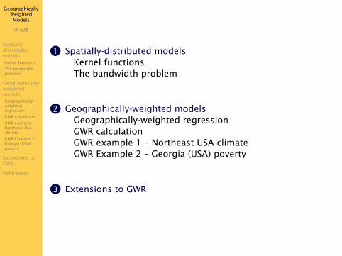
Global model

• GLS: ANN_GDD50 ~sqrt(ELEVATION_) + N

• Fitted coefficients:

(Intercept) 3136.37sqrt(ELEVATION_) -3.00 (per

√m)

N -1.91 (per km)E (not used, does not improve adjusted R2)

spatial correlation of residuals effective range ≈ 52 km

• adjusted R2 ≈ 0.86, RMSE 217 GDD_50

• Interpretation: strong regional effect of elevation andNorthing on the annual heat unitsEasting not significant in the global (regional) model


W'ô




GWR calculation



Extensions toGWR

References

GLS model residuals

Residuals from GLS fit, actual − predicted

●●

●

●

● ●●

●

●

●●

●●

● ●

●

●

●

●

●

●

●

●

●

●

●●●

●

●

●

●

●

●

●

●

●

●

●

●

●

●

●●

●●

●

●●

●

●

●●

●●

●

●

●●

●

●

●

●●

●

●●●

●

●

●

●

●

●

●●

●

● ●

●

● ●●●

●

●

●●●

●

●●

●

●

●

●

●

●

●

●

●

●

●

●

●

●●

●

●●

●

●

●

●

●●

●

●

●●

●

●●●●●

●

●

●

●●

●

●

●●

●●

●

●

● ●●

● ●

●

●

●

●

●

●●

●

●●

●

●●

●

●

●

●

●

●

●

●●

●

●

●

●

●

●

●

●●

● ●

●

●●

●●

●

●●

●

●

● ●

●

●

●●

● ●

●●●●

●

●

●

●

●

●

●●

●

●

●

●

●

●●

●

●

●

●

●

●

●

● ●●●

●

●●

●

●

●

●

●

●

●

●

●

●

●

●

●

●

●

●

●●

●

●

●

●

●

●

●

●

● ●

●●

●●●

●

●

●

●

●

●

●

●

●

●

●

●

●●

●

●

●●

●

●●

●

●

●●

●

●

●

●

●

●●

●

●

●●

●

●●

●

●

●

●

●

●●

●

●

●

−514.041−149.624−3.98160.856653.748

Model was not equally good everywhere! And there are clearclusters of +/- residuals.


W'ô




GWR calculation



Extensions toGWR

References

What to do about this model?

The model is successful over the region, but there areimportant local variations.What to do?

1 Krige the residuals and add to the GLS prediction(GLS-RK)

• This accounts for a local process, within the regionalprocess

• e.g., presence of large water bodies

2 GWR to fit the model locally• Will miss the regional variation• Assumes the process is local• Maybe will better fit locally, and reveal the local importance

of the three predictors

Question: which seems more appropriate in this case?


W'ô




GWR calculation



Extensions toGWR

References

GWR model – select a bandwidth

Use a Gaussian kernel; optimize by cross-validation

fixed 72.4 km• at this radius a point receives e1/2 = 0.6065

weight.• all points will be considered

adaptive 3.35% of the stations in each window, i.e., about10 stations for each regression


W'ô




GWR calculation



Extensions toGWR

References

GWR model – R2

Gauss fixed bandwidth

Coefficient of determination

Fre

quen

cy

0.6 0.7 0.8 0.9

010

2030

4050

Gauss adaptive bandwidth

Coefficient of determination

Fre

quen

cy

0.6 0.7 0.8 0.9

010

2030

40

Regional value shown with red vertical lineMost local models have a poorer fitBecause of the restricted range of predictors in a local window


W'ô




GWR calculation



Extensions toGWR

References

GWR model – intercepts - feature-spacedistribution


Intercept

Den

sity

2500 3500 4500 5500

0.00

000.

0005

0.00

100.

0015


Intercept

Den

sity

2500 3500 4500 5500

0.00

000.

0004

0.00

080.

0012


W'ô




GWR calculation



Extensions toGWR

References

GWR model – intercepts - spatial distribution

Intercept, fixed kernel

2500

3000

3500

4000

4500

5000

Intercept, adaptive kernel

2500

3000

3500

4000

4500

5000

Not the average! A centering constant. Note low values insouthcentral PA & the Taconics as well as northern NY/VT


W'ô




GWR calculation



Extensions toGWR

References

GWR model – elevation - feature-spacedistribution


sqrt(elevation) coefficient

Fre

quen

cy

−50 −45 −40 −35 −30 −25 −20

010

2030

40


sqrt(elevation) coefficient

Fre

quen

cy−50 −45 −40 −35 −30 −25 −20

010

2030

40


W'ô




GWR calculation



Extensions toGWR

References

GWR model – elevation - spatial distribution

elevation coefficient, fixed kernel

−50

−45

−40

−35

−30

−25

−20

elevation coefficient, adaptive kernel

−50

−45

−40

−35

−30

−25

−20

Much of this pattern seems to be an artefact of GWR


W'ô




GWR calculation



Extensions toGWR

References

GWR model – Northing - feature-spacedistribution


N coefficient

Den

sity

−4 −2 0 2 4

0.0

0.1

0.2

0.3

0.4


N coefficient

Den

sity

−4 −2 0 2 4

0.00

0.05

0.10

0.15

0.20

0.25

0.30


W'ô




GWR calculation



Extensions toGWR

References

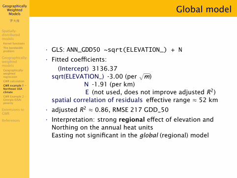
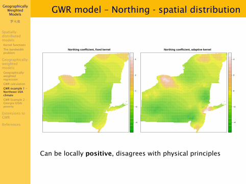
GWR model – Northing - spatial distribution

Northing coefficient, fixed kernel

−4

−2

0

2

4

Northing coefficient, adaptive kernel

−4

−2

0

2

4

Can be locally positive, disagrees with physical principles


W'ô




GWR calculation



Extensions toGWR

References

GWR model – Easting - feature-spacedistribution


E coefficient

Fre

quen

cy

−4 −2 0 2 4 6 8

050

100

150


E coefficient

Fre

quen

cy−4 −2 0 2 4 6 8

020

4060

8010

012

0


W'ô




GWR calculation



Extensions toGWR

References

GWR model – Easting - spatial distribution

Easting coefficient, fixed kernel

−4

−2

0

2

4

6

8

Easting coefficient, adaptive kernel

−4

−2

0

2

4

6

8

Local effect in lower Hudson valley


W'ô




GWR calculation



Extensions toGWR

References

Significance of coefficients

Significance N coefficient

●●

●

●

●●●

●

●

●

●

●

●

●●

●

●

●

●

●

●

●

●

●

●

●●

●

●

●

●●

●

●

●

●

●

●

●

●

●

●

●

●●

●

●

●

●

●

●

●

●●

●

●

●

●

●

●

●

●

●

●●

●●●

●

●

●

●

●

●

●

●

●

●●

●

● ●

●●

●

●

●●

●

●

●

●

●

●

●

●

●

●

●

●

●

●

●

●

●

●●

●

●●

●

●

●

●

●

●

●

●

●●

●

●

●●

●●

●

●

●

●

●

●

●

●●

●

●

●

●

●●

●

● ●

●

●

●

●

●

●

●

●

●●

●

●●

●

●

●

●

●

●

●

●●

●

●

●

●

●

●

●

●

●

● ●

●

●●

●●

●

●●

●

●

● ●

●

●

●●

●●

●

●●●

●

●

●

●

●

●

●

●

●

●

●

●

●

●

●

●

●

●

●

●

●

●

● ●●

●

●

●

●

●

●

●

●

●

●

●

●

●

●

●

●

●

●

●

●

●

●

●

●

●

●

●

●

●

●

● ●

●●

●●

●

●

●

●

●

●

●

●●

●

●

●

●

●

●

●

●

●●

●

● ●

●

●

●●

●

●

●

●

●

●●

●

●

●

●

●

●

●

●

●

●

●

●

Significance E coefficient

●●

●

●

●●●

●

●

●

●

●

●

●●

●

●

●

●

●

●

●

●

●

●

●●

●

●

●

●●

●

●

●

●

●

●

●

●

●

●

●

●●

●

●

●

●

●

●

●

●●

●

●

●

●

●

●

●

●

●

●●

●●●

●

●

●

●

●

●

●

●

●

●●

●

● ●

●●

●

●

●●

●

●

●

●

●

●

●

●

●

●

●

●

●

●

●

●

●

●●

●

●●

●

●

●

●

●

●

●

●

●●

●

●

●●

●●

●

●

●

●

●

●

●

●●

●

●

●

●

●●

●

● ●

●

●

●

●

●

●

●

●

●●

●

●●

●

●

●

●

●

●

●

●●

●

●

●

●

●

●

●

●

●

● ●

●

●●

●●

●

●●

●

●

● ●

●

●

●●

●●

●

●●●

●

●

●

●

●

●

●

●

●

●

●

●

●

●

●

●

●

●

●

●

●

●

● ●●

●

●

●

●

●

●

●

●

●

●

●

●

●

●

●

●

●

●

●

●

●

●

●

●

●

●

●

●

●

●

● ●

●●

●●

●

●

●

●

●

●

●

●●

●

●

●

●

●

●

●

●

●●

●

● ●

●

●

●●

●

●

●

●

●

●●

●

●

●

●

●

●

●

●

●

●

●

●

Significance elevation coefficient

●●

●

●

●●●

●

●

●

●

●

●

●●

●

●

●

●

●

●

●

●

●

●

●●

●

●

●

●●

●

●

●

●

●

●

●

●

●

●

●

●●

●

●

●

●

●

●

●

●●

●

●

●

●

●

●

●

●

●

●●

●●●

●

●

●

●

●

●

●

●

●

●●

●

● ●

●●

●

●

●●

●

●

●

●

●

●

●

●

●

●

●

●

●

●

●

●

●

●●

●

●●

●

●

●

●

●

●

●

●

●●

●

●

●●

●●

●

●

●

●

●

●

●

●●

●

●

●

●

●●

●

● ●

●

●

●

●

●

●

●

●

●●

●

●●

●

●

●

●

●

●

●

●●

●

●

●

●

●

●

●

●

●

● ●

●

●●

●●

●

●●

●

●

● ●

●

●

●●

●●

●

●●●

●

●

●

●

●

●

●

●

●

●

●

●

●

●

●

●

●

●

●

●

●

●

● ●●

●

●

●

●

●

●

●

●

●

●

●

●

●

●

●

●

●

●

●

●

●

●

●

●

●

●

●

●

●

●

● ●

●●

●●

●

●

●

●

●

●

●

●●

●

●

●

●

●

●

●

●

●●

●

● ●

●

●

●●

●

●

●

●

●

●●

●

●

●

●

●

●

●

●

●

●

●

●

red: non-significant; dark green: negative; light green: positive

Intercepts are always highly significant, i.e., 6= 0; they centrethe local regression

Interpretation: most local models are fit only with the localaverage (intercept)!


W'ô




GWR calculation



Extensions toGWR

References

Global vs. GWR model

• Global model finds the average effect, over the entireregion, of the predictors

• the physically-plausible Northing and elevation are highlysignificant

• these have a wide range of values over the region• good fit, over 85% of variance explained

• GWR model:• local models with an effective radius ≈ 100 km• wide range intercepts (averages) → local means

• this takes out most of the effect of Northing• some effect of Northing, Easting near water bodies• elevation only important in windows with significant relief

• usually much lower R2, less of each window is explained byfactors other than the local mean

• In this case the GWR model is not justified.


W'ô




GWR calculation



Extensions toGWR

References

Example – Georgia (USA) poverty

• Georgia (USA) counties 1990 census; originally used in [3]

• Problem: how to explain the proportion of the populationin poverty?

• Possible predictors: percent of population which is:1 rural2 has a bachelor’s degreee or higher3 elderly4 foreign-born5 African-American

• Practical application: if we know what is correlated withpoverty (positive or negative), we can think ofinterventions


W'ô




GWR calculation



Extensions toGWR

References

Global model – computation

## lm(formula = lm.formula, data = educ.spdf@data)#### Residuals:## Min 1Q Median 3Q Max## -7.8282 -2.8418 -0.2404 2.6184 17.4764#### Coefficients:## Estimate Std. Error t value Pr(>|t|)## (Intercept) 7.506033 2.325226 3.228 0.001525 **## PctRural -0.007883 0.015780 -0.500 0.618121## PctBach -0.293767 0.083418 -3.522 0.000566 ***## PctEld 0.709494 0.126583 5.605 9.46e-08 ***## PctFB 0.148516 0.366098 0.406 0.685549## PctBlack 0.259411 0.019638 13.210 < 2e-16 ***#### Multiple R-squared: 0.7078, Adjusted R-squared: 0.6982


W'ô




GWR calculation



Extensions toGWR

References

Global model – interpretation

• about 70% of the variability in poverty is explained.

• The strongest predictors are education (moderatelynegative), elderly (strongly postive), black (moderatelypositive).

• Proportion of rural residents has almost no effect – but isthis because we are mixing urban (Atlanta, Savannah) andrural areas?

• Proportion of foreign-born residents has almost no effect


W'ô




GWR calculation



Extensions toGWR

References

Local statistics

A null model can be used to find locally-weighted statistics of atarget variable.

global mean 70.18 global s.d. 27.1

Note: bounding box about 443 x 514 km


W'ô




GWR calculation



Extensions toGWR

References

Comparing kernels

• GWR depends on the choice of kernel1 functional form2 bandwidth3 fixed vs. adaptive

• Next slides show the difference between kernels


W'ô




GWR calculation



Extensions toGWR

References

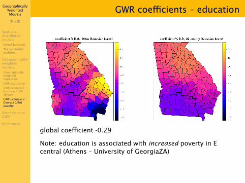
GWR coefficients – education

global coefficient -0.29

Note: education is associated with increased poverty in Ecentral (Athens – University of GeorgiaZA)


W'ô




GWR calculation



Extensions toGWR

References

GWR coefficients – % elderly

Note the increased noise with the narrower kernel.


W'ô




GWR calculation



Extensions toGWR

References

Artefacts – foreign-born


W'ô




GWR calculation



Extensions toGWR

References

Interpretation

• Substantial differences in regression coefficients acrossmap

• In some cases the sign changes

• Suggests different causes/correlations in different areas:look for local effects

• Substantial differences with choice of kernel

• Question: is 50 km with Gaussian weights an appropriatefixed bandwidth?

• Question: are 22 counties with Gaussian weights anappropriate adaptive bandwidth?


W'ô




GWR calculation



Extensions toGWR

References



3 Extensions to GWR


W'ô




GWR calculation



Extensions toGWR

References

Mixed GWR

• GWR model with some coefficients global, i.e., not varyingwith the moving window

• Allows global/regional effects• Example: soil organic matter: affected by regional climate,

but by local topographic effects [9]

• MGWR tests which predictors are fixed and which can vary(and at which bandwidth) [8]


W'ô




GWR calculation



Extensions toGWR

References

Multiscale Geographically Weighted Regression(MGWR)

• Developed by Fotheringham et al. [4]

• GWR with different bandwidths for different processes(represented by predictors)

• computes an optimal bandwidth vector in which eachelement indicates the spatial scale at which a particularprocess takes place

• can interpret the various bandwidths to infer the spatialprocesses


W'ô




GWR calculation



Extensions toGWR

References

Geographically-weighted PCA

• As with OLS regression, but now Principal Components [6]

• Look for the multivariate correlations among predictors ina moving window

• Interpret the PC loadings, per window

• Can use the PC scores to create new, uncorrelatedvariables


W'ô




GWR calculation



Extensions toGWR

References

GW PCA

Georgia poverty predictors, 50 km Gaussian bandwidth

PC1 much more explanatory in NW GA, i.e., predictors aremuch more correlated there


W'ô




GWR calculation



Extensions toGWR

References

Conclusion

• A useful tool to investigate spatial heterogeneity inregression models

• changing coefficients, changing variable importance,changing R2

• the bandwidth reveals the spatial scale of theheterogeneity

• This should be interpretable in terms of thephysical/social setting


W'ô




GWR calculation



Extensions toGWR

References

References I

[1] Roger Bivand. Geographically Weighted Regression. Oct 2017. URLhttps://cran.r-project.org/web/packages/spgwr/vignettes/GWR.pdf.

[2] A. Stewart Fotheringham. Geographically Weighted Regression, pages242–253. SAGE Publications, Ltd, 2009. ISBN 978-1-4129-1082-8. doi:10.4135/9780857020130.n13.

[3] A. Stewart Fotheringham, Chris Brunsdon, and Martin Charlton.Geographically weighted regression: the analysis of spatially varyingrelationships. Wiley, 2002. ISBN 0-471-49616-2. doi:10.4135/9781849209755.

[4] A. Stewart Fotheringham, Wenbai Yang, and Wei Kang. MultiscaleGeographically Weighted Regression (MGWR). Annals of the AmericanAssociation of Geographers, 107(6):1247–1265, Nov 2017. doi:10.1080/24694452.2017.1352480.

[5] Isabella Gollini, Binbin Lu, Martin Charlon, Christopher Brundson, andPaul Harris. GWmodel: an R package for exploring spatial heterogeneityusing geographically weighted models. Journal of Statistical Software,17, Feb 2015. doi: 10.18637/jss.v063.i17.

[6] Paul Harris, Chris Brunsdon, and Martin Charlton. Geographicallyweighted principal components analysis. International Journal ofGeographical Information Science, 25(10):1717–1736, Oct 2011. doi:10.1080/13658816.2011.554838.

https://cran.r-project.org/web/packages/spgwr/vignettes/GWR.pdf

https://cran.r-project.org/web/packages/spgwr/vignettes/GWR.pdf


W'ô




GWR calculation



Extensions toGWR

References

References II

[7] Binbin Lu, Paul Harris, Martin Charlton, and Chris Brunsdon. TheGWmodel R package: further topics for exploring spatial heterogeneityusing geographically weighted models. Geo-spatial Information Science,17(2):85–101, Apr 2014. doi: 10.1080/10095020.2014.917453.

[8] Chang-Lin Mei, Ning Wang, and Wen-Xiu Zhang. Testing the importanceof the explanatory variables in a mixed geographically weightedregression model. Environment and Planning A: Economy and Space, 38(3):587–598, Mar 2006. doi: 10.1068/a3768.

[9] Canying Zeng, Lin Yang, A-Xing Zhu, David G. Rossiter, Jing Liu, JunzhiLiu, Chengzhi Qin, and Desheng Wang. Mapping soil organic matterconcentration at different scales using a mixed geographically weightedregression method. Geoderma, 281:69–82, Nov 2016. doi:10.1016/j.geoderma.2016.06.033.

Documents

Geographically Weighted Models