Embed Size (px)
Citation preview

University of Central Florida University of Central Florida
STARS STARS
Retrospective Theses and Dissertations
1988
Geographic Information Systems: The Developer's Perspective Geographic Information Systems: The Developer's Perspective
Johnn B. Henris University of Central Florida
Part of the Industrial Engineering Commons
Find similar works at: https://stars.library.ucf.edu/rtd
University of Central Florida Libraries http://library.ucf.edu
This Masters Thesis (Open Access) is brought to you for free and open access by STARS. It has been accepted for
inclusion in Retrospective Theses and Dissertations by an authorized administrator of STARS. For more information,
please contact [email protected].
STARS Citation STARS Citation Henris, Johnn B., "Geographic Information Systems: The Developer's Perspective" (1988). Retrospective Theses and Dissertations. 4287. https://stars.library.ucf.edu/rtd/4287
GEOGRAPHIC INFORMATION SYSTEMS: THE DEVELOPER'S PERSPECTIVE
BY
JOHNN B. HENRIS B.S., University of Central Florida, 1987
RESEARCH REPORT
Submitted in partial fulfillment of the requirements for the degree of Master of Science
in the Graduate Studies Program of the College of Engineering University of Central Florida
Orlando, Florida
Fall Term 1988
ABSTRACT
Geographic information systems, which manage data
describing the surface of the earth, are becoming
increasingly popular. This research details the current
state of the art of geographic data processing in terms of
the needs of the geographic information system developer.
The research focuses chiefly on the geographic data
model--the basic building block of the geographic information
system. The two most popular models, tessellation and
vector, are studied in detail, as well as a number of hybrid
data models.
In addition, geographic database management is discussed
in terms of geographic data access and query processing.
Finally, a pragmatic discussion of geographic information
system design is presented covering such topics as
distributed database considerations and artificial
intelligence considerations.
ii
TABLE OF CONTENTS
INTRODUCTION ....
GEOGRAPHIC DATA MODELS.
Vector Models .... Spaghetti Model Topologic Models
Tessellation Models ... Regular Tessellation Models .....• Hierarchical Tessellation Models. Irregular Tessellation Models .•....•.. Scan-line Models ........ . Peano Scan Models ....•......•.
Hybrid Models ... Vaster Model .. Strip Tree Model.
GEOGRAPHIC DATABASE MANAGEMENT.
Geographic Data Access
Query Processing
GEOGRAPHIC INFORMATION SYSTEM DESIGN.
General Design Considerations ..
Distributed Database Considerations.
Artificial Intelligence Considerations
CONCLUSION.
BIBLIOGRAPHY.
iii
1
4
6 8
10
23 24 28 39 45 46
50 51 54
57
59
63
65
65
71
72
76
78

INTRODUCTION
Geographic data processing involves the management of
data describing the surface of the earth. The data involved
describes both natural and man-made features. This data has
traditionally been stored in the form of paper maps and
charts; however, the computer is now becoming an
increasingly important tool for the storage and management
of geographic data. Modern computer technology offers
almost unlimited potential for automating maps and making
them more effective and easier to use.
Computerized geographic data processing involves many
different areas, including geography, cartography, remote
sensing, computer graphics, and many others. All of these
areas come together to form a dynamic and exciting new
science, with great potential for the future.
The chief product to come out of the relatively young
field of computerized geographic data processing has been
the Geographic Information System (GIS). A GIS is a system
of hardware and software components used to manage
geographic data. This report describes the basic technology
behind the geographic information system from the GIS
developer's perspective.

The earliest geographic data processing software was
developed chiefly by geographers and cartographers, as
opposed to computer scientists. This early software,
therefore, tended not to take full advantage of all the
facets of computer science; the algorithms were simple and
straightforward, designed to get the job done. As
geographic data processing grew in popularity, however, a
new breed of geographer appeared on the scene, a
geoprapher/computer scientist. This new professional
brought together the skills necessary to carry geographic
data processing to its present advanced state.
2
The principle factors which aided in the development of
the modern geographer, and in turn of modern geographic data
processing, were the advances in data structure theory and
data modeling theory which occurred in the late 1960's and
early 1970's. These advances fostered the development of
modern database analysis and design, on which geographic
data processing is based.
The material in this report should be considered
essential to both the researcher just beginning in the
geographic data processing field, and the professional
embarking on the design and implementation of a GIS. The
first, and largest, section of the report focuses on the
basic building block of the geographic information system:
3
the geographic data model. Although important to both the
researcher and the professional, this section is probably
most important to the researcher, who will likely spend more
time working at this fundamental level than the
professional.
The next section of the report discusses geographic
database management. As opposed to the previous section,
this section is probably more important to the professional,
since it discusses database management in terms of
geographic data access and query processing.
Finally, a pragmatic discussion of geographic
information system design is presented in the last section.
This material is equally important to both the researcher
and the professional. This discussion includes general
design considerations, distributed database considerations,
and artificial intelligence considerations.
As mentioned previously, computer graphics play an
important role in computerized geographic data processing.
In fact, the graphics capabilities of a geographic
information system are often one of the chief decision
criteria considered by potential users. However, because
this report concentrates on geographic data models, and data
management and design factors directly related to geographic
data modeling, a discussion of computer graphics is not
included.

GEOGRAPHIC DATA MODELS
A data model is an abstraction of reality. It can be
thought of as an intuitive conceptualization of the real
world. A data model is the first of a number of levels of
abstraction necessary to represent real world data in
digital format. Peuquet (1984) describes these levels of
abstraction as:
Reality - the phenomenon as it actually exists, including all aspects which may or may not be perceived by individuals;
Data Model - an abstraction of the real world which incorporates only those properties thought to be relevant to the application or applications at hand;
Data Structure - a representation of the data model often expressed in terms of diagrams, lists, and arrays designed to reflect the recording of the data in computer code;
File Structure - the representation of the data in storage hardware.
These last three levels are precisely the major steps
involved in database design and implementation.
In the past, common usage had tended to consider the
terms "data model" and "data structure" synonymous.
However, advances in data structure theory and computing
technology have fostered the creation of the "level of
abstraction" definition of a data model. Thus, the data
model "has evolved to connote a human conceptualization of
4

reality, without consideration of hardware and other
implementation conventions or restrictions" (Peuquet 1984,
69) •
5
Data modeling is by far the most important component
of database design. There are always a number of ways (file
structures) to represent any type of data in digital form.
The key element which makes this digital data a viable
database, however, is the efficiency with which the data can
be stored and retrieved. It is the data model which
provides the framework for storage and retrieval.
The most common data models in use today are those
used in the processing of non-spatially referenced data.
While the locations in space of geographic entities are the
chief subject of geographic data processing, there is more
to geographic data than just location. Other data
describing non-spatially related details of the entities,
known as attribute data, are better stored using more
conventional non-spatial data models. Examples of these
models are the relational model, the hierarchical model, and
the network model.
Spatially referenced data are the major component of a
GIS, and spatial data modeling is therefore the heart of
geographic data processing. The remainder of this section
details the major developments in the field of spatial data
modeling.

At this point, the reader should note that this
section of the report is an update of Peuquet's 1984
landmark article in Cartographica, entitled "A Conceptual
Framework and Comparison of Spatial Data Models."
6
Since the advent of geographic data processing, two
main data models have been developed for representing
geographic spatial data: vector and tessellation (Figure 1).
Vector and tessellation models are logical duals. In other
words, the basic logical unit of a vector data model is the
map entity for which spatial information is stored, while
the basic logical unit of a tessellation model is a unit of
space for which map entity information is stored.
Vector Models
The basic logical unit of the vector data model is the
single vector, or map line. The vector data model
represents geographic spatial data in terms of three
different elements: points, line segments, and polygons.
A point represents the endpoint of a line segment or
the location of a significant map feature. A feature can be
a mountain, lake, building, or similar object. Points are
also known as nodes, junctions, and intersections.
A line segment represents the line connecting two
nodes. Note that a line segment does not represent the
shape of the line; that is defined separately. Line
segments are also known as arcs, edges, faces, and links.

Fig. 1.
Analog
Original Contour Map t y
Vector
Vector Organization
(basic element= line)
Tessellation
Grid Organization
(basic element •
grid vertex or grid cell)
t y
t y
.... ~ , ..
~ .., L) j
I I I\
l \ \ l ""'
I\ r- ...
r", -
x-
x-
... - ....
~ '\ ~
......... _ ... ~ ""'
( ~ 1 I
- ...__ I f
r-... 'J
-~"' ,-- II' IJ "'-- VL..o ....
Geographic data models. (Peuquet 1984)
7

A polygon represents the smallest area formed by a
connected set of line segments. Polygons are also known as
areas and regions.
Spaghetti Model
8
The simplest form of the vector data model is known as
the "spaghetti model." It is a direct line-for-line
translation of a paper map in which each entity on the map
becomes a separate logical record in the digital file.
Entities are represented as connected series of line
segments. The line segments are stored by recording the x-y
coordinates of their endpoints in the digital file, as shown
in Figure 2. A polygon is stored as a closed loop of line
segments. The occurrence of adjacent polygons, therefore,
introduces data redundancy in the spaghetti model because
the line segments shared by adjacent polygons are stored
twice.
In the spaghetti model, the map remains the conceptual
model, and the x-y coordinate file is actually a data
structure. Although the entities themselves are spatially
defined, the relationships between them are not retained.
The spaghetti model is therefore simply a collection of
coordinate strings grouped together with no inherent
structure.

9
( Data Model)
Data Structure Feature Number loc111on
Poinl 10 X, Y (Single Point)
Line 23 x1 v1 .~ v2 ....... Xn Yn (String)
63 x1 v1 .x27, ...... x1 v1 (Closed Loop)
Polygon
64 x1v1.xl2, ...... x1v1(0ata Slructure)
Fig. 2. Spaghetti model. (Peuquet 1984)
10
The lack of an implicit unifying structure makes the
spaghetti model extremely inefficient for analytical
purposes. Spatial relationships between entities must be
computed using complicated algorithms. The model, however,
is well suited for graphic output operations because the
missing structural relationships are unnecessary to the
output process. As a result, the spaghetti model is only
used in simple geographic data processing functions which
involve little or no analysis.
Topologic Models
The topologic model is the most common vector data
model in use today. Based on the principles of graph
theory, the topologic model "defines a location of
geographic phenomena relative to other phenomena, but does
not require the use of the concept of distance in defining
these relationships" (Dangermond 1982). In other words, the
topologic model retains the relationships between entities
by explicitly storing adjacency information.
Figure 3 shows an example of a topological model
(called a topologically coded network map). Two separate
files comprise the model. One file stores the coordinates
of the network's line segment endpoints, or nodes; the other
stores each line segment along with references to its
endpoint nodes and to the polygons which appear to the left

Coded Network Map
Right Link -,. PolyQon
1 1 2 2 3 2
" 1 5 3 6 3 7 5 8 " 9 5
10 .. 11 0
e
Left PolyQon Node 1 Node 2
0 3 1 0 " 3 , 3 2 0 1 2 2 " 2 0 2 5 3 5 8 3 e ' .. 7 e 0 7 4 5 5 7
Topologically Coded Network & Polygon File
Node# X Coordinate Y Coordinate
1 23 a 2 17 17 3 29 15 .. 26 21 5 e 28 6 22 30 7 24 38
X,Y Coordinate Node File
Fig. 3. Topologic model. (Peuquet 1984)
11
12
and right of it. The basic spatial relationships between
entities are implicit in the topologic model. This greatly
enhances the usefulness of the model in analytical
functions. Furthermore, data redundancy, as can occur in
the case of adjacent polygons, is eliminated.
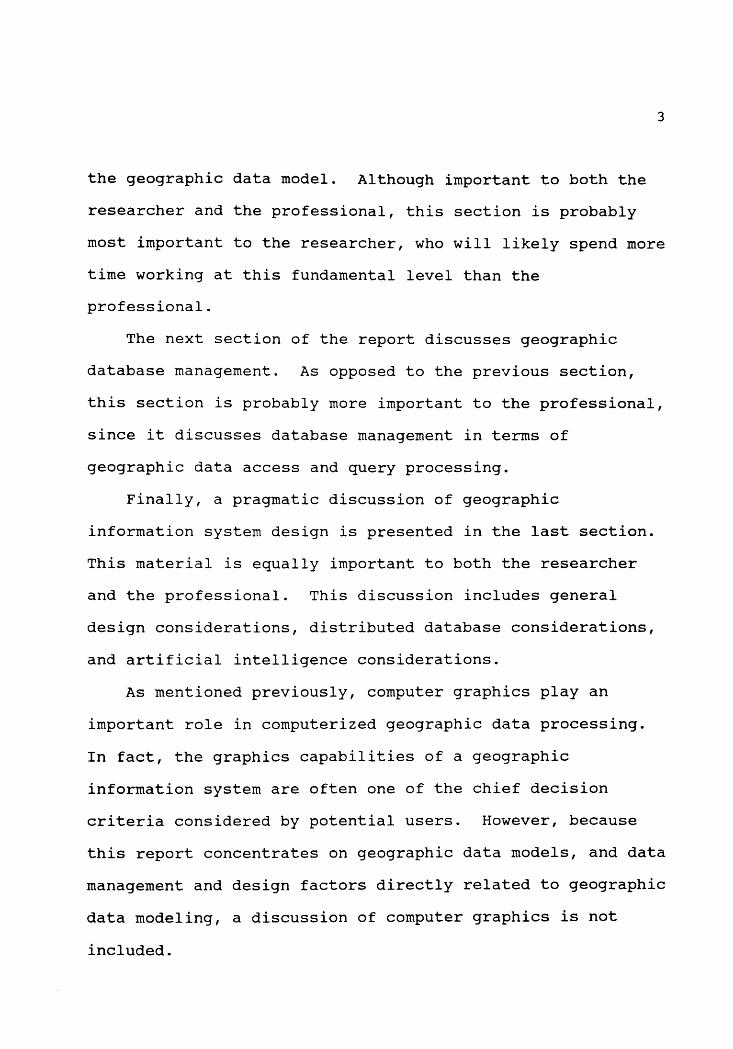
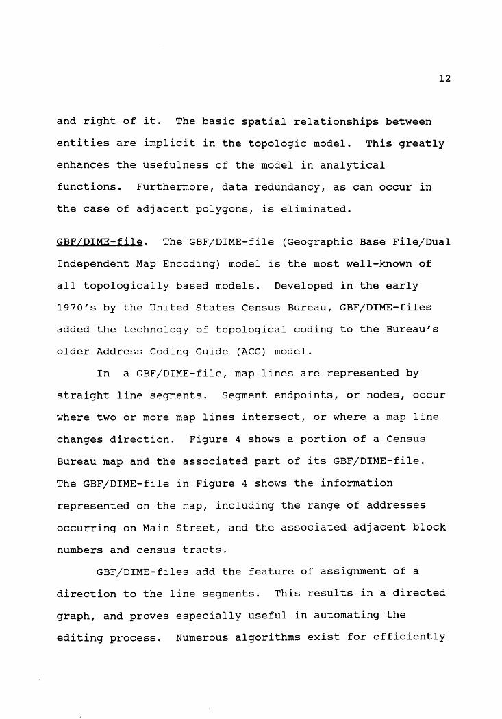
GBF/DIME-file. The GBF/DIME-file (Geographic Base File/Dual
Independent Map Encoding) model is the most well-known of
all topologically based models. Developed in the early
1970's by the United states Census Bureau, GBF/DIME-files
added the technology of topological coding to the Bureau's
older Address Coding Guide (ACG) model.
In a GBF/DIME-file, map lines are represented by
straight line segments. Segment endpoints, or nodes, occur
where two or more map lines intersect, or where a map line
changes direction. Figure 4 shows a portion of a Census
Bureau map and the associated part of its GBF/DIME-file.
The GBF/DIME-file in Figure 4 shows the information
represented on the map, including the range of addresses
occurring on Main Street, and the associated adjacent block
numbers and census tracts.
GBF/DIME-files add the feature of assignment of a
direction to the line segments. This results in a directed
graph, and proves especially useful in automating the
editing process. Numerous algorithms exist for efficiently

tracing directed graphs and therefore the computer can
automatically check for missing line segments and other
errors.
13
The chief disadvantage of the GBF/DIME-file model is
that the line segments are not stored in any particular
order. To retrieve a line segment, an exhaustive search
must be performed on the entire file. To retrieve all the
line segments associated with a polygon, the exhaustive
search must be performed as many times as there are segments
in the polygon.
TIGER File. The TIGER (Topologically Integrated Geographic
Encoding and Referencing) file data model is a new
topologically based model being developed by the United
States Bureau of the Census (Marx 1986). The TIGER file
model is being designed to take full advantage of the
science of graph theory. The TIGER file model is one of the
best examples of the topological model in actual practice
and so will be described in detail.
The basic elements of the TIGER file model are the
points, line segments, and polygons mentioned previously.
In the TIGER file model, however, these elements are
referred to as a-cells, 1-cells, and 2-cells. These names
arise from the dimensions of the elements; a point is a
zero-dimensional object; a line segment is a one-dimensional
object; a polygon is a two-dimensional object.

The TIGER file model consists of lists of 0-cells,
1-cells, and 2-cells, along with directories which are
matched to the 0-cell and 2-cell lists. Directories are
stored as B-trees, an efficient data structure which
optimizes storage and retrieval.
14
The 0-cell files, namely the 0-cell list and its
directory, contain the coordinates of the line segment
endpoints and features on the map. The 0-cell directory has
a one-to-one correspondence with the o-cell list; each
directory entry has a pointer to its corresponding entry in
the 0-cell list.
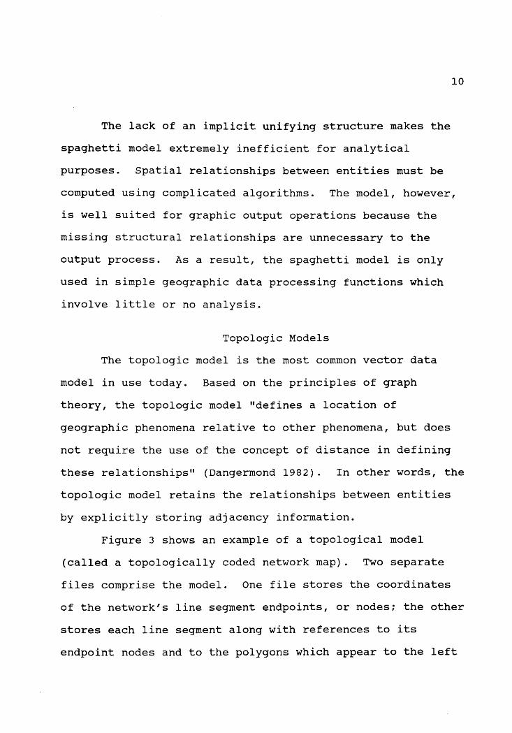
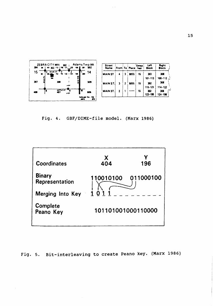
The 0-cell directory aids in the quick retrieval of
the nearest point in the TIGER file given any point on the
map. The TIGER file model uses a Peano key indexing system
based on bit-interleaving to accomplish this. A Peano key
is created by merging alternate binary bits from the
latitude and longitude values of the given point. This
creates a new unique binary number which is used as an index
into the one-dimensional 0-cell directory (Figure 5).
Two-cells are the areas enclosed by connected series
of 1-cells. Two-cells are also stored in terms of a 2-cell
directory and a 2-cell list. Groups of 2-cells are often
grouped together into what are known as "coverages." These
aggregate 2-cells aid in large scale data tabulation
operations.
ZEBRA CITV 88!f.> JQ2 1 Adams Twp~ l04 ■ 111 J0l nJ fll 111 z, ,■ Jl1 502
15 • "".t.JIISl J 2 1 14 ■ IIC .. ftl N 1%2 I I~ 1■ -
JD7
-l * I [ -
~11 t «17 .....
StrHt 1 1 1 1c-.1 Left
Name I Ft-om I To ; Place• T..s . Bl<Kk
MAINST.1 • I l ; ass 15 303
101-113
3 2 I USS I MAIN ST 15 302 115-121
I MAJN ST. 2 , - 15 302 123-199
Fig. 4. GBF/DIME-file model. (Marx 1986)
X 404
V 196
flieht J llock
30I i, I
100-112 J 301 I
\ 11,-122
JOI 124-191
Coordinates
Binary Representation
110010100 011000100
Merging Into Key
Complete Peano Key
I~ 1011 ________ _
101101001000110000
Fig. 5. Bit-interleaving to create Peano key. (Marx 1986)
15

16
The 1-cells represent map lines and are the most
important element of the TIGER file model. There is not a
directory for the 1-cell list because access to this list is
obtained by referring to the endpoints of a 1-cell (the
a-cells), the surrounding 2-cells, or the non-topologically
referenced attribute data associated with a group of
1-cells.
Often, certain information is common to a number of
1-cells. In these cases, the information is stored
separately and the 1-cell records contain pointers to it.
One-cell records also contain information on their shapes.
This data is stored in a curvature list file. This file
contains coordinates which completely describe the shape of
a 1-cell. This includes what is known as the envelope of
the 1-cell, which is the rectangle that encloses the 1-cell
with its intermediate curvature coordinates (Marx 1986).
A unique feature included in the TIGER file model,
which greatly increases its efficiency, is the use of a
technique known as "threading." In threading, each a-cell
entry points to no more than one 1-cell, no matter how many
map lines may actually intersect at that point. The 1-cell
record then contains pointers to any other 1-cells which may
occur at that point, and those 1-cells to still others.
This technique reduces computer storage requirements and
also helps alleviate the retrieval problem associated with
the GBF/DIME-file model.

17
The use of directories for accessing TIGER file
records greatly enhances the efficiency of the TIGER file
model. A directory only needs to contain two fields per
entry: the unique reference to the a-cell or 2-cell itself,
and the pointer to the record in the corresponding list.
The list can then grow quite large and contain many data
fields. Because the directory stays small, it can be
quickly searched, and access to any a-cell or 2-cell is
still fast, regardless of the amount of data associated with
it.
DLG-3. The DLG-3 (Digital Line Graph 3) model is a fully
topologic external data exchange structure, as opposed to
the TIGER file model, which is an internal applications
structure.
The major components of the DLG-3 model are the node,
line, and area, which are analogous to the a-cell, 1-cell,
and 2-cell of the TIGER file model. The model centers
around the line. Line records contain pointers to nodes and
areas. The model is designed to "provide the minimal
information needed for a topological structure" (Marx 1986,
198) .
Topologic models are popular because they are based on
the well-developed mathematics of graph theory. The three
topologic models cited in this section, GBF/DIME-file, TIGER

file, and DLG-3, show the integral part that topologic
modeling has played in geographic data processing and the
part it will play in the future (Figure 6 provides a
schematic comparison of these models). The GBF/DIME-file
model has been, and still is, the most commonly used
topologic model. The TIGER file model, with its improved
technology, represents the future of topologic modeling.
Finally, the DLG-3 model, with its simple but complete
topologic basis, has become the closest thing to a
geographic data exchange standard.
POLYVRT. The POLYVRT (POLYgon conVeRTer) topologic data
model was developed at Harvard University in the late
1970's. It is the technology developed in this model which
provided the basis for the TIGER file model mentioned
previously.
18
The POLYVRT model introduced the concept of
threading. In doing so, the model eliminated the need for
the exhaustive search necessary in the GBF/DIME model. The
POLYVRT model also added the advantage that queries
involving polygon adjacency need only deal with the polygon
and [threaded] chain data. Actual coordinate data need not
be retrieved until explicitly needed, such as for distance
calculations and plotting. This is another one of the
advantages apparent in the TIGER file model.
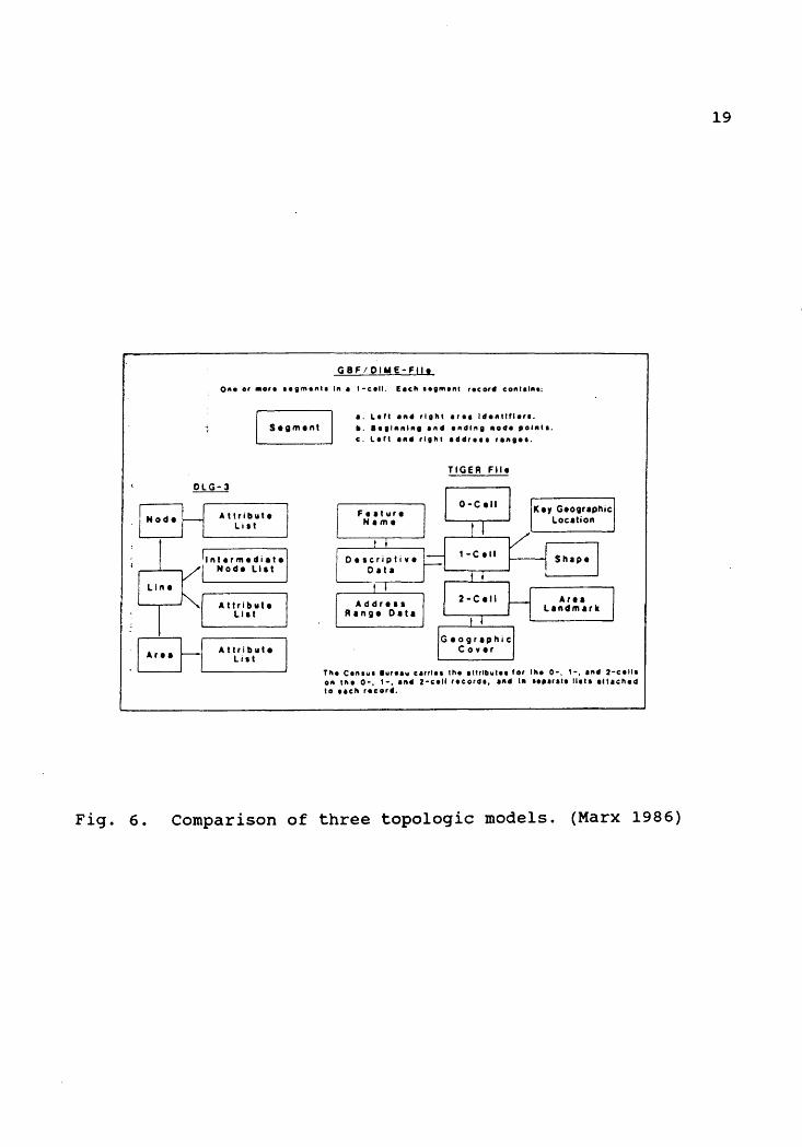
Fig. 6.
Node
GBFIOIME·Fllt
O11e or •ore 1eamen11 In e I ·cell. Eecll 1egme111 ,ecor411 contel11•:
Segment
At tribut • List
Intermediate Node Llat
Attribute List
Attribute Lill
a. Left 811411 rlgl'lt area lde11tlflert. •. ••1111111111 end endln1 IIOIU 11011111. c. L•rt a11411 ,19111 addre11 ra119e1.
Feature Name
TIGER FIie
~ Ker Geographic ~ Location
=l !•Coll H Shapa
Geographic Cover
Are a Landmark
TIie Cen1u1 luree11 cerrte1 11,e 11trtt111te1 for Ille 0•. 1•, end 2·cet11 011 111e O•, 1•, and 2•cetl record1, a11d 111 ••111r111 11111 attaclled to e1cll racorf.
Comparison of three topologic models. (Marx 1986)
19
20
Chaincodes. Chaincodes are, technically, not a data model;
they are more precisely a method of data compaction.
However, chaincode techniques have proved invaluable to
spatial data handling and have come to be viewed as a data
model in their own right (Peuquet 1984).
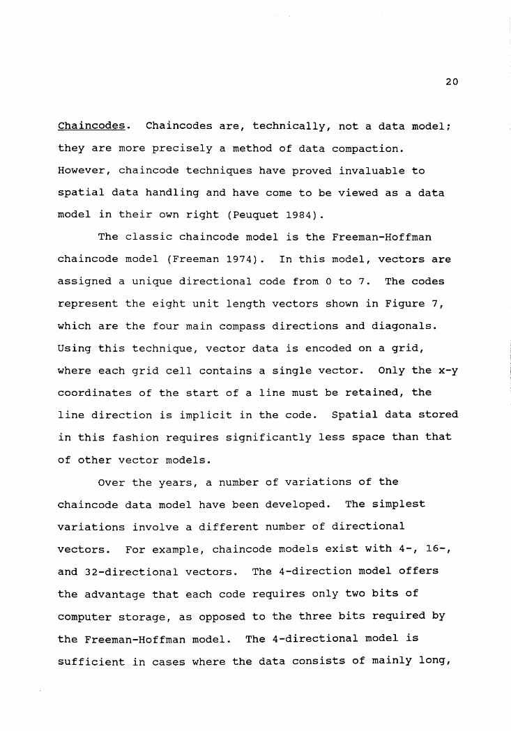
The classic chaincode model is the Freeman-Hoffman
chaincode model (Freeman 1974). In this model, vectors are
assigned a unique directional code from o to 7. The codes
represent the eight unit length vectors shown in Figure 7,
which are the four main compass directions and diagonals.
Using this technique, vector data is encoded on a grid,
where each grid cell contains a single vector. Only the x-y
coordinates of the start of a line must be retained, the
line direction is implicit in the code. Spatial data stored
in this fashion requires significantly less space than that
of other vector models.
Over the years, a number of variations of the
chaincode data model have been developed. The simplest
variations involve a different number of directional
vectors. For example, chaincode models exist with 4-, 16-,
and 32-directional vectors. The 4-direction model offers
the advantage that each code requires only two bits of
computer storage, as opposed to the three bits required by
the Freeman-Hoffman model. The 4-directional model is
sufficient in cases where the data consists of mainly long,

21
straight lines which are perpendicular to one another. The
16- and 32-directional models are better suited to data
which consist of arbitrary-shaped curves. The increased
number of directions available in these models helps smooth
out the staircase effect introduced when models with fewer
directions are used. The disadvantage of the 16- and
32-directional models, however, is that they require more
storage space and so do not provide as much compaction. In
fact, there is a direct relationship between the number of
directions in a chaincode model and the unit vector length
required for any given accuracy. Peuquet points out that,
"in terms of compaction, this obviously presents a tradeoff
between the number of direction-vector codes required to
represent a given line and the number of bits required to
represent each code" (Peuquet 1984, 83).
Another variation of the chaincode model which has
gained acceptance is the Raster Chaincode, or RC Code,
model. The raster chaincode model was designed to process
data in raster order (in horizontal strips, moving one strip
at a time from top to bottom, scanning each strip left to
right). As shown in Figure 8, this method requires only
half the directional vectors of the previously mentioned
chaincode models. One difficulty associated with the raster
chaincode model, however, is that directional continuity of

22
.,, ' 0 I I I o
2 el l ~' 2 \l I I/ 0 .2.~ ~o o:/
2 lY - ':~-r 0 0 0 lY yy 0 0 a- ti.
2 2 Ye ' I 7. ~
y 2 ~--
.. /J .. 't: .. 2 LI. .. -~~ -,Iii. •2 4 2 A ·~·i. ~ ' -
l,( -2 0 0 0 ,, 4 Va 4 I
2 A: o- - --I
2 A I
' , I
Fig. 7. Chaincode model. (Peuquet 1984)
3 2
Fig. 8. Raster chaincode model. (Peuquet 1984)

23
arbitrary lines is not preserved. Fortunately, this problem
is easily solved by a simple conversion from RC code to
Freeman-Hoffman chaincode format.
The compaction ability afforded by chaincode models
makes them especially useful in encoding the huge amounts of
data occurring in modern geographic data processing. Also,
certain measurement and analytical procedures can be
performed more efficiently on chaincoded data.
The major disadvantage of chaincode models is that
they cannot retain spatial relationships; they are, in fact,
compact spaghetti models. For this reason, chaincode models
are most often used in conjunction with other spatial data
models which preserve spatial relationships.
Tessellation Models
Tessellation data models are the logical dual of
vector data models. The basic logical unit of a
tessellation model is a unit of space, as opposed to the map
entity, which is the basic logical unit of a vector data
model. Although the more technical term "tessellation" is
used throughout this report, the reader should note that the
term "raster" has come to be synonymous with the term
"tessellation" and so appears quite often in the
literature. Tessellation models occur in three basic forms:
regular, hierarchical, and irregular. In addition,

scan-line and Peano scan models are commonly classified as
tessellation models and so will be discussed in this
section.
Regular Tessellation Models
24
A regular tessellation model is one in which the
tessellation, or grid, is composed of cells which are of
equal size and shape. There are three types of regular
tessellations: square, triangular, and hexagonal (See Figure
9) •
Square Tessellations. The square tessellation model is the
oldest and most common of all tessellation models. Its
development can be attributed to two factors. First, the
square grid is compatible with the array data structure
common to most programming languages. Second, the square
grid is compatible with most common methods of geographic
data capture and display (Peuquet 1984).
A square tessellation model can best be thought of as
a checkerboard-like matrix, or grid. Individual grid
elements are addressed with an X,Y coordinate pair, with the
lower left corner of the matrix being the origin, o,o. The
X value locates an element along the horizontal axis and the
Y value along the vertical axis. It should be noted that
the origin does not have to be in the lower left corner; it
can in fact be located anywhere on the grid. However, for

the purposes of this example, the lower left corner is the
best location for the origin because all elements can then
be addressed with positive X and Y values only.
25
The size of a square tessellation data model's grid
elements can vary from quite small to extremely large. The
difference is apparent in the resolution offered by the
model and the amount of storage space required for the
model. To illustrate these differences, the reader can
imagine a clear plastic overlay, with grid cells etched into
it, laid over a map.
If the etched grid elements are very small, the
overlay corresponds to a square tessellation model with a
high resolution. The reader can imagine that the grid
elements which are positioned over map lines are colored
in. The clear overlay is then a tessellated representation
of the map. This is essentially the method which raster
scanners use to input data from analog maps.
If the etched grid elements are quite large, the
overlay corresponds to a square tessellation model with a
low resolution. In this case, far too many map lines occur
in any one grid element to allow representation like that in
a high resolution grid. Instead, grid elements can be
assigned aggregate values representing the major quality or
qualities within the element. For example, if the area
within a grid element consists of 45% marsh and 55% forest,

the grid element will be assigned a value representing
forest. This is the method which is used by most remote
sensing devices.
Apart from resolution, the chief difference between
square tessellation models with small and large grid
elements is the amount of storage space each requires.
26
While the grid elements in both models require about the
same amount of space per element (each consists of a simple
code), the number of elements is drastically different. A
square tessellation model with small grid elements requires
more storage space than one with large elements because more
small elements are needed to represent any given area.
Triangular Tessellations. Triangular tessellation models,
both regular and irregular, possess the quality that the
triangles do not all have the same orientation. This makes
triangular tessellation models particularly well suited for
representing terrain and other surface data. The
disadvantage of this quality, however, is that certain
operations involving single cells, which are easy to perform
on the square and hexagonal tessellations, are more
difficult on a triangular tessellation.
A surface is represented in a triangular tessellation
by assigning an elevation value to each triangle vertex (See
Figure 10). Note that the same surface data could be

represented by assigning a slope and direction to each
triangle face. Clearly, each of these representations can
be derived from the other.
27
Although it has been proven that the interpolation of
surface contours is easier using a regular tessellation
(Bengtsson and Nordbeck 1964), regular triangular
tessellations are rarely used for surface data. Irregular
triangular tessellations are far more common. This is
probably because surface data are not usually captured in a
regular spatial sampling pattern.
Hexagonal Tessellations. Regular hexagonal tessellation
models possess the unique feature of radial symmetry (all
neighboring cells of a given cell are equidistant from that
cell's centerpoint). The hexagonal model, therefore, is
particularly well suited to radial search and retrieval
procedures.
Specific details of the geographic data processing
algorithms used on the three regular tessellations differ,
as the geometries of the three polygons differ. Certain
procedures are more straightforward on one tessellation than
on others; however, equivalent algorithms for each of the
three tessellations have been shown to have the same order
of complexity (Ahuja 1983).
28
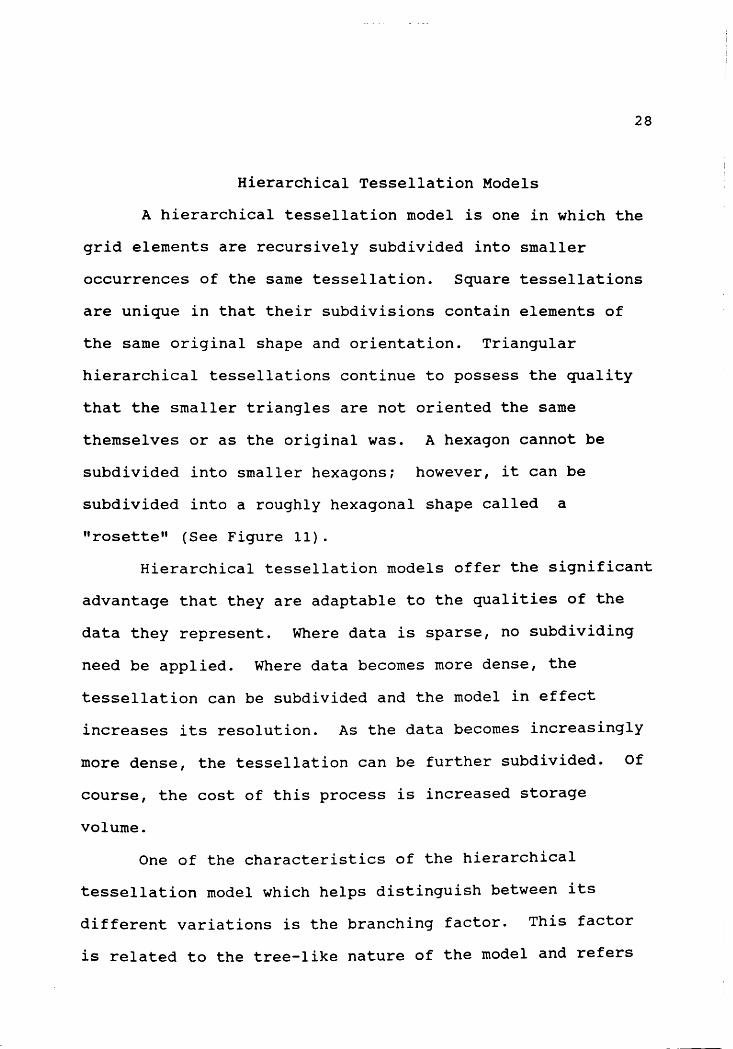
Hierarchical Tessellation Models
A hierarchical tessellation model is one in which the
grid elements are recursively subdivided into smaller
occurrences of the same tessellation. Square tessellations
are unique in that their subdivisions contain elements of
the same original shape and orientation. Triangular
hierarchical tessellations continue to possess the quality
that the smaller triangles are not oriented the same
themselves or as the original was. A hexagon cannot be
subdivided into smaller hexagons; however, it can be
subdivided into a roughly hexagonal shape called a
"rosette" (See Figure 11).
Hierarchical tessellation models offer the significant
advantage that they are adaptable to the qualities of the
data they represent. Where data is sparse, no subdividing
need be applied. Where data becomes more dense, the
tessellation can be subdivided and the model in effect
increases its resolution. As the data becomes increasingly
more dense, the tessellation can be further subdivided. Of
course, the cost of this process is increased storage
volume.
One of the characteristics of the hierarchical
tessellation model which helps distinguish between its
different variations is the branching factor. This factor
is related to the tree-like nature of the model and refers

29
Fig. 9. Regular tessellations. {Peuquet 1984)
Fig. 10. Triangular tessellation. (Peuquet 1984)
.l SQU¥t b. triangular c. roselle
Fig. 11. Regular tessellation subdivisions. (Peuquet 1984)
30
to the number of subtrees a node possesses. The storage
requirement of a hierarchical tessellation model is directly
related to the branching factor.
Square Hierarchical Tessellations. The most common
hierarchical tessellation model in use today is the
quadtree, which is based on the regular square
tessellation. The basic quadtree model can be divided into
three types: point quadtrees, area quadtrees, and line
quadtrees. The reader should note that the term "quadtree"
has also come to be used today in a general sense, referring
to all hierarchical tessellation models.
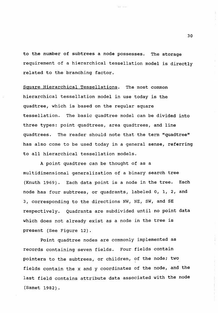
A point quadtree can be thought of as a
multidimensional generalization of a binary search tree
(Knuth 1969). Each data point is a node in the tree. Each
node has four subtrees, or quadrants, labeled O, 1, 2, and
3, corresponding to the directions NW, NE, SW, and SE
respectively. Quadrants are subdivided until no point data
which does not already exist as a node in the tree is
present (See Figure 12).
Point quadtree nodes are commonly implemented as
records containing seven fields. Four fields contain
pointers to the subtrees, or children, of the node; two
fields contain the x and y coordinates of the node, and the
last field contains attribute data associated with the node
(Samet 1982).

(5., l4S)
DEMVER
...
c2s,3s) 1
OM/\HA
(35., llO)
CHICAGO
(50.,10)
(60.,75) TORONTO
(80.,65) BUFFALO
(85.,15) ATLAtff A
MOB I LE r-------_.,_ _ __,
(90.,5) MIAMI
CHICAGO
Fig. 12. Point quadtree. (Samet 1983}
31

32
Quadrants 1 and 3 are closed with respect to the x
coordinate and quadrants O and 2 are closed with respect to
they coordinate. This convention enables the model to
handle cases in which a data point falls exactly on a
quadrant boundary line (Samet 1982).
The area quadtree is similar in concept to the point
quadtree. The root node of an area quadtree represents the
entire region in question -- more precisely a square
entirely containing the region. The four subtrees of the
root represent the NW, NE, SW, and SE quadrants of the root
node. Quadrants are recursively subdivided until all four
subquadrants can be assigned binary values dependent upon
whether or not the subquadrant entirely contains or does not
contain a portion of the original region (See Figure 13).
Area quadtree nodes are usually implemented as records
containing six fields. Four fields contain pointers to the
children of the node, one field contains a pointer to the
parent of the node, and one field contains associated
attribute information (Samet 1982).
Although point quadtrees and area quadtrees are
similar in many respects, there is one fundamental
difference between the two. Whereas the area quadtree works
with fixed partitions, the data determines how the point
quadtree will partition space.

a,. Region
ll 11 1' 14 lS 20 21 6 1 9 10
l s ' 1
11 17
24 30
40 41 4l
b. Block decomposition of the region in (a).
26 27 31 32 21 29 ll 34 JS 36 l8 39
c. Quadtree representation of the blocks in (b).
Fig. 13. Area quadtree. (Samet 1983)
33

34
Line data has proved to be more difficult to represent
with hierarchical tessellation models. Since the early
1980's, however, a number of models have been developed
which are beginning to solve this problem.
The edge quadtree is a hierarchical tessellation model
used to represent line data (Shneier 1981). The edge
quadtree is similar to both the point and area quadtrees.
Like the point quadtree, the edge quadtree partitions
quadrants in order to reference specific data points, namely
the points of the line (locations where the line changes
direction or where two or more segments intersect). Like
the area quadtree, the partitions are fixed and of equal
size (See Figure 14).
Among other problems, the edge quadtree suffers from
an inability to handle, except with the simplest of
solutions, cases in which two or more edges meet at a
single point. Numerous variations of the edge quadtree have
been developed to solve this and other problems associated
with hierarchical tessellation based models of line data.
Clearly, this is one of the many areas of geographic data
processing still requiring further research.
The strip tree is another model being used to
represent line data. Although the strip tree might be
classified as a hierarchical tessellation model, it is more
commonly classified as a hybrid, and so will be discussed in
the Hybrid Data Models section.

35
f G
I .
J
L
A 8
Fig. 14. Edge quadtree. (Samet 1986)

36
Triangular Hierarchical Tessellations. Hierarchical
tessellation models based on the triangular tessellation are
equivalent to the models based on the square tessellation
just described--both models have a branching factor of
four. The triangular model is in fact called a triangular
quadtree. The triangular quadtree has the same advantages
and disadvantages of the regular triangular tessellation,
combined with the advantages of the hierarchical tree
structure.
Hexagonal Hierarchical Tessellations. The hierarchical
tessellation model based on the hexagonal tessellation is
known as the septree. This model has a branching factor of
seven. The model therefore requires a base seven addressing
scheme known as Generalized Balanced Ternary (GBT). The
advantage of this scheme is that many calculations may be
performed directly on the GBT addresses without conversion.
The model suffers from the disadvantage that because a
hexagon cannot be subdivided into smaller hexagons, the
resolution of the tessellation must be predetermined.
Multiple Dimension Hierarchical Models. Although the
examples of hierarchical tessellation models cited so far
deal in only two dimensions, each model can be generalized
ton dimensions. Of course, doing so would cause the

37
branching factor to become very large (i.e., at least 2k for
k dimensions). The model would then require significantly
more storage space.
The multi-dimensional k-d tree (Bentley 1975) offers
an improvement on the quadtree by avoiding the complicating
growth of the branching factor. The k-d tree is essentially
a binary search tree with the distinction that areas are
divided into two parts instead of four. The direction of
the division is alternated with successive levels of the
tree. For instance, in the case of two dimensions, space
could be divided in the x direction on even levels of the
tree, and they direction on odd levels (Samet 1986).
Hierarchical Model Implementation. The hierarchical
tessellation models described have commonly used pointers in
the implementation of their tree structures. However,
recent implementations of the models have begun to use
direct addressing schemes instead of pointers. These models
have been termed linear quadtrees. The name is derived from
the fact that a direct addressing scheme allows the data to
be physically organized in a linear fashion, as in a list.
Linear quadtrees offer the advantage of more efficient
data storage. Nodes in a linear quadtree are arranged in a
list, and each node has a key which uniquely identifies it.
Keys are created by a technique known as bit interleaving.

When sorted in ascending order on the key value, the node
list will be in an order identical to that which would be
obtained from a top-to-bottom traversal of the tree (Samet
1986). Also, the node list is usually stored in a B-tree
data structure, which further improves the model's
efficiency.
38
The tree-like nature of hierarchical tessellation
models makes them especially efficient for procedures which
involve search. The tree structure of these models serves
as a pruning device on the amount of search required for a
given query. Furthermore, the tree data structure is among
the most well documented and researched in computer
science. Numerous algorithms exist for quick, efficient
processing of trees.
Another advantage of hierarchical tessellation models
is that they lead to aggregation. "Aggregation is an
abstraction through which relationships are treated as
higher level entities" (Korth and Silberschatz 1986). The
result of this is that algorithms that use hierarchical
tessellations have execution times proportional to the
number of aggregated units rather than to the actual size of
the aggregated units (Samet 1986).
39
Irregular Tessellation Models
An irregular tessellation model is one in which the
grid elements vary in size, orientation, and density over
space. The three most common irregular tessellation models
in use today are the square, triangular, and variable (or
Thiessen) models.
Irregular tessellation models share one of the
advantages of hierarchical tessellation models. Namely,
irregular tessellation models are adaptable to the qualities
of the data they represent. By stipulating that each grid
element hold the same amount of data, the model can be made
to reflect the density of the data. Where the data is
sparse, the grid elements will be bigger. Where the data is
dense, the grid elements will be smaller. In addition,
irregular tessellation models have the advantage that,
because each grid element is different, the need for
redundant data is eliminated.
Square Irregular Tessellations. The square irregular
tessellation model is the least popular of the irregular
models. The main reason for its unpopularity is the "saddle
point problem" (Mark 1975). This is a problem which often
arises when drawing contour lines on a square irregular
tessellation. A saddle point is a point on a surface for
which the graph of the surface lies on both sides of the
40
tangent plane to the point. The occurrence of saddle points
causes ambiguity in the tracing of contour lines.
Triangular Irregular Tessellations. The triangular
irregular tessellation model, also known as the triangulated
irregular network (TIN), is by far the most common of the
irregular models (See Figure 15). TINs enjoy a number of
advantages over regular tessellation models. For one, TINs
have been shown to result in more accurate surface
representations while requiring less storage space (Mark
1975; Peucker et al. 1976). Also, TIN surfaces can be
generated much faster than regular tessellation surfaces
(Mccullagh and Ross 1980). This is because most topographic
surfaces are highly irregular, and fitting a regular
tessellation grid to an irregular surface requires extensive
interpolation of the original data--an expensive process in
terms of processing time (McKenna 1985).
A significant drawback to the use of regular
tessellation models is the fact that they cannot represent
vertical surfaces, irregular boundaries, or interior surface
holes. TINs, however, can easily represent all of these
features. Furthermore, the resolution of a regular
tessellation model is limited by the resolution of the
superimposed grid, while TIN resolutions are only limited by
the resolution of the data (McKenna 1985).

41
Fig. 15. Triangulated irregular network. (Peuquet 1984)

42
In addition to the advantages described above, TINs
also have a unique property, described by McKenna as
underutilized, which should prove very useful in GIS display
operations. "The irregular nature of the TIN allows the
surface to be freely manipulated and edited" (McKenna 1985,
946). This means that surface points can be moved, added,
and deleted without affecting the data structure of the
original surface.
The main disadvantage of triangulated irregular
networks is that there are many possible triangular networks
which can be generated from the same set of point data.
There are, therefore, many different triangulation
algorithms for a single surface.
Variable Irregular Tessellations. The variable irregular
tessellation model, also known as the Thiessen Polygon
model, is the logical dual of the triangular irregular
tessellation model. Thiessen polygons are formed by
bisecting the side of each triangle in a TIN at a 90 degree
angle. The result is an irregular polygon grid composed of
convex polygons having a variable number of sides (See
Figure 16).
Each convex polygon in a Thiessen grid possesses a
unique control point (the center of mass) which is actually
the original TIN data point. The grid is partitioned such

43
Fig. 16. Thiessen polygon network. (Monmonier 1982)
44
that each convex polygon is the collection of points lying
closer to the control point of that region than to any other
control point (Monmonier 1982). An alternate logical
derivation of a Thiessen polygon grid is based on this
quality. Given a finite number of data points (at least
three) distributed in a bounded plane, each point begins to
propagate a circle at a constant rate. These circles
continue to grow until one circle encounters another or the
boundary of the plane. The result is a Thiessen polygon
grid (Rhynsburger 1973).
Thiessen polygons are also known as Voronoi diagrams
or dirichlet tessellations. Thiessen polygons were first
applied in the determination of recipitation averages over
drainage basins by A.H. Thiessen in 1911, after whom they
were named (Rhynsburger 1973).
One particularly useful advantage of irregular
tessellation models stems from the ability of the size,
shape, and orientation of their grid elements to reflect the
size, shape, and orientation of the actual data elements.
This quality proves very useful in visual inspection and
related operations.
Although irregular tessellation models are well suited
to a few specific procedures, such as visual inspection,
they are, as a rule, not good general spatial data models.

There are two chief reasons for this. First, irregular
tessellations are extremely hard to generate; they are
complex and take a good deal of computer time. Second,
overlaying of two or more tessellations, one of the most
basic geographic data processing operations, is difficult
and sometimes even impossible when dealing with irregular
tessellations.
Scan-line Models
45
Scan-line, or raster, models are compact versions of
the more traditional regular tessellation data model. The
main difference between the two model types is that the grid
elements of the scan-line model are swaths of the data
surface. Although these swaths, or rows, are usually
oriented horizontally, they do sometimes appear vertically.
The compaction feature of the scan-line model arises
from the way in which the model forms the scan-line rows.
Rows can be thought of as lists of regular tessellation grid
elements. The grid elements which do not contain a map
entity, or any piece of a map entity, are discarded. The
scan-line row, then, consists of only the essential grid
elements -- no empty elements.
The main disadvantage of scan-line models is that they
do not preserve vertical relationships between scan-line
rows. Although some procedures can operate on the data in

this compact form, procedures which involve any vertical
relationships between scan-line rows cannot. In these
cases, the data must be converted back into grid form.
Peano Scan Models
46
Peano scan models, or space filling curves, convert
n-dimensional space into a one-dimensional line, and vice
versa. Peano curves accomplish this by tracing an unbroken
line through space. These curves possess three primary
properties, described by Stevens, Lehar, and Preston (1983):
1. The unbroken curve passes once through every locational element in the dataspace.
2. Points close to each other in the curve are also close to each other in space, and vice versa.
3. The curve acts as a transform to and from itself and n-dimensional space.
Figure 17 provides examples of two-dimensional and
three-dimensional Peano curves.
Peano curve models were first implemented in the
geographic data processing field within the Canada
Geographic Information System (CGIS) (Tomlinson 1973). This
implementation is based on a Z-shaped Peano curve. The
curve divides space into "unit frames." The frames are
referenced using an indexing scheme known as the Morton
matrix (Morton 1966). Figure 18a presents a portion of the
Morton matrix indexing scheme, and Figure 18b shows the

47
Fig. 17. 2- and 3-dimensional Peano curves. (Peuquet 1984)

48
0 2 3 X )
0 0 2 8 10 32 34 40 42 0000 0010 1000 1010
1 3 9 l 1 33 35 41 43 0001 0011 1001 t011
2 4 6 12 14 36 38 44 46 0100 0110 1100 1110
3 5 7 13 15 37 39 45 47 0101 0111 1101 1111
1 16 18 24 26 48 50 56 58
l 17 19 25 27 49 51 57 59
20 22 28 30 52 54 60 62
21 23 29 31 53 55 61 63
Fig. 18a. Morton matrix indexing scheme. (Peuquet 1984)
X
0 1 2 3 4 5 6 7
0
1
2
3 y
4
5
6
7
Fig. 18b. z-shaped Peano curve. (Peuquet 1984)

relationship between the Morton matrix and the z-shaped
Peano curve.
49
The Z-shaped Peano curve has a direct correspondence
with the quadtree data model. Specifically, by using the
bit interleaving indexing technique, a unique address can be
generated for a grid element from the elements binary X and
Y coordinates. When converted to base 4, the address
corresponds to the location of the same element in a base 4
indexed hierarchical tessellation grid (a quadtree).
In summary, vector and tessellation models both have
advantages and disadvantages associated with them. Neither
model is ideal for all applications.
Vector data models are direct digital translations of
lines from a paper map. Therefore, vector algorithms also
tend to be direct translations of traditional manual
methods. Consequently, these algorithms have been
well-developed. The chief disadvantage of vector models is
that spatial relationships between map entities must be
explicitly stored.
Tessellation data models, on the other hand, contain
spatial relationships implicitly. Also, they are compatible
with methods of high-speed input and output. The major
disadvantage of tessellation data models, however, is that
they take up a great deal of storage space. Furthermore,
tessellation algorithms are less developed than vector
algorithms, although this fact is changing quickly.
Hybrid Models
50
Recently, a great deal of research has gone into
resolving the classic storage and processing tradeoffs which
exist between the vector and tessellation data models. One
approach has been to store geographic data in tessellation
format and convert it to vector format only when absolutely
necessary. This technique is popular because it is
intuitively straightforward; however, conversion between
data models can quickly become an insurmountable bottleneck.
Although conversion from vector format to tessellation
format is fast and efficient, conversion in the other
direction is quite a different story. Conversion from
tessellation format to vector format requires some form of
intricate line-following because cartographic lines are
characteristically complex and unpredictable. This process,
therefore, entails significant overhead and its use needs to
be limited.
Another approach to the tradeoff problem between
vector and tessellation data models has been to develop
tessellation-based algorithms which are as fast and
efficient as their vector counterparts. This combination
would capture the advantages of both data models in a single
[tessellation] model and would eliminate the need for vector

data models. In fact, many efficient tessellation-based
algorithms have already been developed (especially within
the field of image processing), but there are still some
processes which seem to be intrinsically vector-oriented.
Furthermore, certain procedures, such as network
shortest-path and optimal-routing, are so much more
efficiently performed in vector format that even the added
cost of conversion makes them desirable over the most
efficient tessellation-based algorithms (Peuquet 1984).
51
Perhaps a better solution to the vector/tessellation
problem than those just mentioned is the use of hybrid data
models which incorporate characteristics of both the vector
and tessellation data models. The remainder of this section
will describe some of the recent developments in the area of
hybrid data model design.
Vaster Model
The basic idea of the vaster data model is the storage
of cartographic data in the tessellation-based form of
horizonatal swaths, or rasters, and the storage of data
within each swath in vector format (See Figure 19) (Peuquet
1982). The vaster model, therefore, removes the need for
conversion between tessellation and vector formats.
Specifically, the leading edge (line corresponding to
minimum y value) of a swath is stored in raster format and

x-y~-::--..-r-r--r:""-r-r:---r,-,-r---r----------1
1 -1~ : ♦ , •
1 • • Swatrl I
Swath 3: x-
y
l t· ; Li.
Swath 4:
~---41~-· ----------.. J ·-~ ' ~ } ~~ . -}~-·
- scan line dat.t
}-_,, ....
x-y __ ___. __ _,._ _ __.~...,...~_.,...,._ __ .__.,..... ____ _,_ ~n line dal.t
l ~ • j
Fig. 19. Vaster data model. (Peuquet 1984)
52

53
is used as an index into the swath itself. This is
accomplished by associating an identifier and x-value with
each intersection of a map line with the leading edge.
Polygons and lines which appear in but do not intersect the
raster are stored seperately but still within the swath
record. This intra-swath data is stored in compact
chain-coded vector format.
The vaster data model can thus be used at two
different resolutions. The first, coarser resolution is
realized by using only the tessellation-based raster
structures. This resolution is useful for browsing and for
a great deal of general applications where approximate
solutions are required. These include centroid, area,
perimeter, and arc-length calculations.
The second, full-detail resolution available with the
vaster data model makes use of the vector data within each
raster. A complete vector representation of the data can be
constructed by rectifying the indices of the rasters. The
data would then be suitable for more detailed analysis.
Fully realizing the potential of the vaster data model
to combine the advantages of both the tessellation and
vector data models, however, involves solving a couple of
related problems. First, there is the data sampling problem
analogous to the grid cell size problem associated with
tessellation data models. What size should the rasters be
54
so as to most efficiently represent the data at the coarser
resolution? If rasters are too big, many map lines and
entities will be "stranded" and representable only in vector
format. If the rasters are too small, map lines will be
intersected many times and the model will become
unmanageably large. Ideally, "each significant map line
should be intersected at least once by a scan line ... "
(Peuquet 1984, 104).
The second problem involved in implementing the vaster
data model arises from the hybrid nature of the model. What
raster/vector data volume ratio would provide optimum
performance given the set of raster and vector algorithms
necessary for the intended applications (Peuquet 1984)?
Concentrating data in vector format when the application
uses mainly raster algorithms, for instance, would hardly be
considered optimal.
Strip Tree Model
The strip tree data model represents geographic data
by using a hierarchy of bounding rectangles (Samet 1982).
The strip tree is classified as a hybrid data model because
its basic logical entity is the map line, but the lines
themselves are not explicitly recorded. This representation
allows optimum performance of union, intersection, and curve
length operations.

55
Individual strips, or segments of a line or curve,
consist of four elements: El, E2, Wl, and W2. El and E2 are
points locating the beginning and end of the strip,
respectively. Wl and W2 denote the right and left distances
of the strip borders from the directed line segment (See
Figure 20).
A strip tree for a given line segment between two
points is formed by first finding the smallest bounding
rectangle between the two points. Next, a point which
touches one of the two sides of the rectangle is selected
and the process is repeated for the two sublists. The
result is two subtrees which are children of the original
line segment, or root node. This process is terminated when
the lowest level rectangles reach a predetermined size.
The strip tree model can be thought of as the vector
counterpart to the quadtree data model since each is based
on the hierarchical structure of the underlying map entity.
The main difference between the two, however, is that
quadtrees must be spatially registered before they can be
used in most processes but strip trees can be arbitrarily
translated and scaled since they are grid independent.

I\
D o n
C

GEOGRAPHIC DATABASE MANAGEMENT
The sheer volume of geographic data available today,
and the magnitude of the tasks required of today's
geographic data processing systems, demands the optimum
performance from geographic database management systems.
Intricate data models, such as those described in the
previous section, can be devised to very acurately represent
large geographic areas. However, the real test of a
geographic database is how easily this data can be
maintained and how efficiently it can be accessed in
processing queries.
Geographic database queries involve requests for data
which are subject to two types of constraints. The first
type deals with spatial data. This is data which represents
the actual location in space of a map entity. The second
type of constraint deals with attribute data. This is the
non-spatially registered data associated with a map entity.
Attribute related constraints can usually be handled easily
with simple table lookups. Spatially related constraints,
however, typically involve some manipulation of vector or
tessellation data. Combining these two types of constraints
can lead to complex queries. For example, consider the
following sample query:
57

Find the locations of all parcels of land within a 25 mile radius of Orlando, FL which are less than 50% developed, hold more than 5 lakes, and do not contain at least 2 intersecting state roads.
The above query specifies two attribute related
58
constraints. The first stipulates that parcels be less than
50% developed, and the second that five or more lakes be
located on the parcel. The query also specifies the spatial
constraint that the parcels lie within a 25 mile radius of
Orlando, FL. The last constraint specified by the query
could be either attribute or spatially related. If the
original designers of the database anticipated queries about
intersections of state roads, they might have included an
attribute in parcel records which represented the number of
state road intersections in that parcel, in which case the
query processor has simply to read this attribute. However,
if state road intersection data is not included as an
attribute of parcels, then the DBMS must perform a spatial
analysis routine to determine which, if any, state roads
intersect on each parcel it checks.
This simple example introduces a couple of important
points relating to geographic database management which will
be discussed in this section. These points have to do with
the methods used to access geographic attribute and spatial
data, and methods for efficiently processing both
anticipated and unanticipated queries.

59
Geographic Data Access
Spatial geographic data and its related attribute data
are stored separately. Although this practice may not be
intuitively straightforward, it greatly increases the
efficiency of the geographic database. This is because many
geographic data processing functions are performed using
only one of these two datasets at a time.
Geographic attribute data is far easier for the
geographic data processing system to manipulate than
geographic spatial data. Most geographic data processing
systems now use the relational data model to store and
maintain attribute data. These systems either maintain
themselves, or offer access to, a fully developed relational
data management system for this purpose.
The relational data model has been well studied and
documented. The literature abounds with material on the
subject and therefore the model will only be discussed here
in terms of how it is being used in the field of geographic
data processing.
For the storage and maintenance of attribute data, a
geographic database management system associates attribute
data (stored in a relational database) with spatial data
through a linking mechanism. A code, such as a simple
numbering scheme, is usually used for this purpose. For
example, consider the imaginary system which was queried
60
earlier in this section. Assume each parcel of land is given
a unique parcel number. Then a relational table called
"Parcel" can be created with parcel number being the key.
The parcel table can then be used to store attributes such
as percentage of development, number of lakes, and number of
intersecting state roads (all information used by the
earlier sample query). The parcel number is the key which
associates spatial and attribute information.
As was described in the section on Data Models, the
science of geographic spatial data modeling has not yet been
fully developed. For that reason, the methods for accessing
geographic spatial data, both vector and tessellation based,
are not as well developed as those for accessing non-spatial
data.
At the lowest level, the vector data model is very
similar in appearance to the relational data model.
Geographic spatial data stored in vector format occurs in
the form of tables (arc, node, and polygon tables), similar
to the relational data model. For this reason, many
geographic data processing systems on the market today use a
relational database system to implement a vector spatial
data model. The most notable of these are ESRI's Arc/Info
and Arc/Oracle systems.

61
Spatial data, however, is fundamentally different from
the data which is usually managed by relational database
management systems. Specifically, the concept of dimension
introduces complex relationships among spatial data entities
which are not easily represented by conventional relational
database systems. For this reason, the relational database
management systems used to manage vector data, such as those
in Arc/Info and Arc/Oracle, are adapted versions of the
conventional relational data model. Recently, a great deal
of research has been devoted to normalizing spatial data to
allow future spatial data models to fully utilize the rich
theory of relational data modeling (van Roessel 1986).
Because the basic logical entity of the tessellation
data model is the unit of space, tessellation data is
accessed quite differently than vector data. While vector
data tables offer natural indices on spatial data and bounds
on the amount of search required for most operations,
tessellation data models typically do not. Tessellation
data, therefore, must be accessed by referring to specific
data cell addresses as opposed to referring to specific map
entities.
The addressing schemes used to access tessellation
data range from very simple, such as the X,Y coordinate
pairs used with the square tessellation grid, to complex,
such as the GBT scheme used with the septree model.

It is important to note, however, that these addressing
schemes do not aid in searching for specific geographic
entities; in this case, tessellation data must usually be
searched sequentially.
62
Another method which can greatly increase the
efficiency of accessing a large geographic database is the
use of a virtual memory system. Virtual memory describes a
set of techniques which allow a system to execute a program
(or in the case of geographic data processing, display a
map) which is not entirely in memory at the time (Peterson
and Silberschatz 1985).
A virtual memory system essentially works by storing
in main memory the data which it anticipates is likely to be
required. In other words, if, in a GIS which utilizes
virtual memory, a user requests a certain map parcel to be
displayed, the system may load in that parcel and all
parcels which border it, anticipating that the user will
wish to view data only in this area. If the user wishes to
access data which is not currently in memory, the system
uses one of a number of methods to determine a portion of
the data currently in main memory to remove and replace with
the required data.
63
Query Processing
In the process of designing a geographic data
processing system, the developers will certainly have in
mind a number of standard queries, or types of queries,
which they are fairly certain will be posed frequently. The
developers may therefore choose to augment the system in
some way which will help it process these standard queries
as efficiently as possible. There are three common methods
for achieving this goal: indexing, hashing, and clustering.
Indexing and hashing are very common in the
conventional database field. They both involve the addition
of structures to the data model which improve retrieval
efficiency for a specific dataset (i.e., a relational data
table). The disadvantage of these methods is the increased
overhead involved with their implementation. However, their
benefits far outweigh their costs. For further information
regarding indexing and hashing, the reader is referred to
Korth and Silberschatz (1986).
Clustering refers to the process of storing related
data contiguously in memory. This allows data to be
accessed more efficiently than if it were distributed in
memory. Clustering, like indexing and hashing, is also very
common in the conventional database field. For further
information, the reader is referred to Korth and
Silberschatz (1986).

64
Although the methods mentioned above are often
implemented in the database design phase, they are also used
in the day-to-day operation of the database. One or more of
the three can be temporarily implemented to optimize
processing of queries which may not have been anticipated by
the system designers. The lives of these temporary aids may
be as short as one query, or they may be left as permanent
additions to the database.
GEOGRAPHIC INFORMATION SYSTEM DESIGN
Geographic data processing and geographic database
management share with the more traditional database
management field at least one very important quality--the
design phases of both the database and the Database
Management System (DBMS) are the most crucial factors
affecting the life of the system. Calkins reports that "in
the software development field it has been shown that fully
65% of the errors found during implementation and testing of
a system can be traced to poor design" (Calkins 1983, 92).
In fact, there have been numerous system failures in the GIS
field and this has led to the creation of a "credibility
gap" between the promoters of geographic data processing
systems and the people who most benefit from their
existence--the users (Marble and Peuquet 1983).
General Design Considerations
An organization embarking on the design of a GIS will
certainly have in mind a number of basic requirements for
the new system. However, the GIS developers will not want
to limit the growth potential of an expensive, long-lived
piece of software such as a GIS. Therefore, they will
65

66
likely develop as general a set of specifications as
possible. In this way, the developers can attempt to allow
for future implementation of new methods and technologies,
assuring an efficient, productive life for the GIS.
Although speaking in such general terms about the
requirements of the GIS makes it appear that the system
could live up to any and all expectations, there is a danger
involved here. A loose set of specifications means that
there will be no clear idea of when an adequate design has
been reached (Calkins 1983). This is one of the classic
pitfalls of database design and it played a major role in
the GIS system failures mentioned at the beginning of this
section.
So what can the developers do when they truly do not
have a definite set of specifications for their GIS? There
are two options available here. Either they could decide
upon a definite set of specifications--a subset of the very
general class which has been discussed so far, or they can
proceed with the general class of specifications--working
carefully to avoid the problem discussed in the preceeding
paragraph. Deciding on a limited set of specifications
essentially defeats the purpose of the long-term goals for a
GIS. So the answer seems to be: implement the most general
system available, with the plan that the system can be
67
continually updated as new requirements are adopted and new
technology is developed.
By planning to implement the most general system
available, however, the developers again face the problem of
too general a scope. Clearly, this danger is in part
unavoidable. However, there are other factors which affect
the quality of a database which are more in contol of the
designers. Chief among these factors is the design of the
database itself.
Accurate modeling of real-world relationships within
attribute datasets is the most important part of the design
phase of a GIS--and in fact of any database system. This is
not to play down the importance of spatial data modeling,
but the relationships between spatial data entities are far
more straightforward than those between non-spatial data
entities. Futhermore, the attribute and spatial data
modeling disciplines are at quite different levels of
development.
In a still developing field like spatial data
modeling, there is always the possibility that a
revolutionary new discovery will come along which would
render current methods obsolete. On the other hand,
attribute data modeling technology, especially the
relational data model, is well established. Therefore,

additional time and effort devoted to the attribute data
modeling process would help guarantee the usefulness and
long lifespan of a GIS.
68
The usefulness and effectiveness of the GIS will be
directly related to the extent to which the GIS is linked to
existing and future non-geographic databases used by the
organization. The most advanced GIS, possessing
state-of-the-art analysis and display capabilities, is
nothing more than a glorified map viewing device if it is
not linked to the existing databases within the organization
implementing it. In such a situation, the only way to make
the GIS effective, apart from going back to square one and
creating the links, involves duplicating already existing
data. This introduces data redundancy, an ailment which
wastes valuable memory space and complicates database
maintenance.
As a simplified example of the advantage of links to
existing databases, consider the case of an imaginary market
research firm which is planning to implement a new GIS.
Imagine that the firm has extensive data about consumers and
products at different cities around the country.
The firm's GIS could be designed to include a U.S. map
dataset consisting chiefly of spatial data. This would
include data which facilitated detailed spatial analysis and

69
output of maps of any portion of the U.S. There would be a
minimum of attribute data associated with this U.S.
geography dataset, the idea here being that existing
non-geographic databases, such as the consumer and product
databases of the previous paragraph, could be linked to this
dataset to act as attribute data. Specifically, the city
name could be used as a code to link consumer data contained
in the existing database to point data in the U.S. geography
dataset--namely the city locations.
Making the consumer information database act as
attribute data for a U.S. geography database, then, opens up
new possibilities for market queries. For example, users
could compute travel times between consumer groups and
product distribution sites, or optimize distribution within
a network of sites. Also, comparison of spatially based
data from different sites could be performed easily.
An approach similar to the scenario described above
would minimize the effort required to implement a GIS,
promote data independence, and prevent data redundancy, the
last two factors being of critical importance to assuring a
long life for the GIS.
Accordingly, during the process of designing the GIS
and its related components, a significant amount of effort
should be devoted to determining where links exist which

70
could tie existing database elements to the new GIS. The
fact that this attribute data can be fully normalized
according to the techniques of relational data modeling
guarantees that it will be useful in satisfying the general
specifications written of earlier.
As far as geographic spatial data modeling is
concerned, the choice of a spatial data model is almost
irrelevant--stress almost. Certainly, in terms of getting a
GIS up and functional as quickly as possible, a spatial data
model, or more to the point, a fully operational GIS with
supporting spatial data model, must be decided upon.
However, the organization needs to approach the
implementation of their GIS with the knowledge that, in the
event that the original spatial data model needs to be
updated or replaced, their sizable investment in spatial
attribute data is safe.
All this is not to say that a commercially available
GIS on the market today could not be implemented by the
organization and function effectively for many years.
However, in a situation where the original specifications
(by necessity) are very loose, and where such a large
investment in already existing databases could be at stake,
responsibility dictates that the worst case scenario must be
considered.

71
Distributed Database Considerations
The large size of a GIS and its associated components
makes it an ideal candidate for implementation as a
distributed database. A distributed database is one that
consists of a collection of sites, each of which maintains
its own local database system. Sites may process local
transactions, those that access data located only at that
site, or global transactions, those that access data located
at a number of different sites (Korth and Silberschatz
1986) .
By maintaining site specific geographic (and
non-geographic) data at the actual site location, the
organization could assure the timely and accurate update of
its entire geographic database. Distribution is also more
economically feasible than maintaining the entire geographic
database at one location. In order to be maintained at one
location, such a large database would require a sizable
investment in hardware, software, and personnel.
Although distribution of a GIS would be beneficial in
terms of data sharing, data reliability, and speedup of
query processing, there would also be disadvantages
associated with it. Specifically, increased software
development costs, greater potential for bugs, and increased
processing overhead are problems associated with database
distribution.

72
Artificial Intelligence Considerations
Artificial Intelligence (AI) can best be described as
"the study of how to make computers do things at which, for
the moment, people are better" (Rich 1983, 1). AI has
received a great deal of publicity lately, and research is
being conducted which attempts to apply AI techniques to
almost all forms of data processing--geographic data
processing is no exception.
The most useful development to stem from the field of
artificial intelligence has been the expert system. An
expert system is a computer system which assists in the
solution of real-world problems which require an expert's
knowledge to solve. An expert system uses a computer model
of expert human reasoning to arrive at the same conclusion
which the human expert would, given the same information
(Weiss and Kulikowski 1984).
The most important characteristic of an expert system
is that it is based on a large database of knowledge. An
expert system's knowledge base consists of two types of
knowledge: facts and rules. Facts are, as the name implies,
declarative facts regarding the problem domain. Rules are a
mechanism for control. A rule consists of a left side and a
right side. The left side is a pattern to be matched
against a problem state; the right side is a change to be
made to the current problem state. For example, an expert
73
system for identifying animals might have in its knowledge
base a rule such as: "If the animal in question bears live
young, then the animal is a mammal." The left side of the
above rule is that part which appears before the comma, the
right side is that part which appears after the comma.
Very few, if any, artifical intelligence applications
for general spatial data processing are developed enough yet
to be of practical use. This fact, however, does not mean
that applications for artificial intelligence (specifically
the expert system) do not exist within more specific domains
of spatial data processing and attribute data processing.
Expert systems which deal with non-spatially
referenced (attribute) data are far more developed than
those that deal with spatially referenced data. The
likelihood that there is already a large amount of attribute
data existing in any organization and the importance of that
data to a new GIS make the implementation of expert systems
dealing with this data an option worth considering.
The possible applications of expert systems to
attribute data are as varied as the applications of the
GIS. However, generally speaking, any organization involved
in geographic planning and decision-making has experts whose
experience helps them make sound decisions. In arriving at
their conclusions, these experts deal almost exclusively
with attribute data. This is not to say that spatial data
74
is not required--indeed, spatial data is the heart of
geographic data processing--but almost all spatial data can
in essence be boiled down into attribute data.
This last point is precisely the main point made in
the geographic database management section: if the GIS
developer determines that certain spatial data
characteristics will be required often, he can represent
them as attribute data. Therefore, in the simplest example
of a GIS expert system, every constraint within the
left-hand side of a rule would simply correspond to some
data field within the GIS's attribute database.
Clearly, a system configured as that described in the
previous paragraph would defeat the purpose of a GIS--there
would be no need for a spatial data model. A more realistic
system would allow certain constraints within the left-hand
sides of rules to be fulfilled by queries to the spatial
data model. For example, consider the hypothetical expert
system rule which states: "If all the parcels of land within
a 25 mile radius of Orlando are more than 50% developed,
then consider expansion of Orlando area utility services."
A simple spatial analysis routine can identify those parcels
which are geographically located within a 25 mile radius of
Orlando. Then, a quick table lookup identifies those
parcels which are more than 50% developed.

75
Since it is now clear that there is indeed potential
for the expert system within a GIS, and that the combination
is technically feasible, the main issue then becomes the
development of the knowledge base. This is in fact the main
issue involved in the implementation of an expert system in
any field.
The building of the knowledge base is the chief
bottleneck in the implementation of an expert system. And
yet, this will always be the case, since an expert system's
usefulness and efficiency are directly related to the amount
of work put into the building of its knowledge base.
Translating the knowledge of one or more experts into
a form suitable for use in an expert system requires a great
deal of careful, patient effort. This effort, or at least
part of it, could be incorporated into the system design
phase which an organization carries out long before they
implement a GIS. This is not to say that effort should be
wasted on trying to develop (too soon) an expert system with
the loose set of requirements which were discussed earlier.
Indeed, one fact is certain: an expert system must be based
on a rigorously structured set of requirements. However,
the organization should keep in mind that the "rules" they
use throughout the course of their work in modeling
real-world spatial entity and attribute relationships are
precisely the rules which a future expert system would use.
CONCLUSION
Computerized geographic data processing is still a
relatively young science; and yet, the chief product to come
out of the field, the Geographic Information system (GIS),
is already a great commercial success. Advances in GIS
technology are occurring regularly, and the future of the
GIS, and its supporting industry, appears bright.
This report has presented the most basic technology
behind the geographic information system. The material
covered in this report should be considered essential by
both researchers just entering the geographic data
processing field, and professionals embarking on the design
and implementation of a GIS.
The first, and largest, part of the report concentrated
on the basic building block of geographic information
systems: the geographic data model. The two main types of
geographic data models, vector and tessellation, were
presented and examined in detail. In addition, a discussion
was included which described hybrid data models--models
which attempt to capture the advantages of both the vector
and tessellation models.
The next section of the report discussed geographic
database management in terms of geographic data access and
76

query processing. This section concentrated on factors
which affect the day-to-day performance of a geographic
information system.
77
Finally, the last section of the report presented a
pragmatic discussion of geographic information system
design. This section developed a short, "real-life"
scenario to stress the importance of the design phase to the
performance of a database system. The section also
presented discussions on distributed database considerations
and artificial intelligence considerations in the design of
a geographic information system.
The field of geographic data processing is a complex and
dynamic one. The researcher or professional working in the
field needs to devote considerable effort to the "education
process," both initially and throughout their work. This
report has hopefully served that purpose--to provide the
researcher or professional with the basic knowledge
necessary to study and develop geographic information
systems.
BIBLIOGRAPHY
Abel, S.R., and H.A. Griesemer. 1985. Virtual image mapping and multi-plane image construction enhance performance of a terrain display system. In Geographic Information Systems in Government, Vol. 1 (Proceedings of a workshop in Springfield, Virginia 10-13 December 1985], edited by B.K. Opitz, 237-244. Hampton, VA: A. Deepak Publishing.
Ahuja, N. 1983. On approaches to polygonal decomposition for hierarchical image decomposition. Computer Vision, Graphics, and Image Processing 24: 200-214.
Bengtsson, B., ands. Nordbeck. 1964. Construction of isarithms and isarithmic maps by computers. Nordisk Tidschrift for Informations-Behandling 4: 87-105.
Bentley, J.L. 1975. Multidimensional binary search trees used for associative searching. Communications of the ACM (September): 509-517.
Calkins, H.W. 1982. A pragmatic approach to geographic information system design. In The Design and Implementation of Computer-Based Geographic Information Systems [Proceedings of a U.S./Australia workshop in Honolulu, Hawaii 1982], edited by D. Peuquet and J. O'Callaghan, 92-101. International Geographical Union.
Campbell, W.G., G.D. Bishop, M.R. Church, J.J. Lee, D.A. Lammers, and L.H. Liegel. 1987. The Environmental Protection Agency's direct/delayed response project: The role of a geographic information system. In GIS '87, Vol. 2 [Proceedings of a conference in San Francisco, California 26-30 October 1987], by American Society for Photogrammetry and Remote Sensing. 456-467. Falls Church, VA: American Society for Photogrammetry and Remote Sensing.
Carter, J.R. 1984. Computer Mapping Progress in the '80s. Washington D.C.: Association of American Geographers.
78

79
Dangermond, J. 1982. A classification of software components commonly used in geographic information systems. In The Design and Implementation of Computer-Based Geographic Information Systems (Proceedings of a U.S./Australia workshop in Honolulu, Hawaii 1982], edited by D. Peuquet and J. O'Callaghan, 70-91. International Geographical Union.
Faintich, M.B., J. Simley, and R. Fortson. 1984. Terrain elevation and surface feature data display for mission, land use, and trafficability planning. In Pecora 9 [Proceedings of a conference 2-4 October 1984], by The Institute of Electrical and Electronics Engineers. 278-285. Silver Spring, MD: IEEE Computer Society Press.
_____ . 1984. Interactive analysis of digital terrain elevation and surface feature databases. Photogrammetria 39: 85-90.
Faust, N. 1988. Presentation at a geographic data processing symposium. University of Central Florida, 8 July 1988.
Foresman, T.W. 1987. Present and future role of GIS technology for hazardous waste facility management. In GIS '87, Vol. 2 [Proceedings of a conference in San Francisco, California 26-30 October 1987], by American Society for Photogrammetry and Remote Sensing. 468-475. Falls Church, VA: American Society for Photogrammetry and Remote Sensing.
Freeman, H. 1974. Computer Processing of Line-drawing Images. Computing surveys 6: 57-97.
GIS WORLD, Inc. 1988. GIS WORLD 1, No. 1 (July).
Goodwin, C. 1987. The on-line atlas: a GIS for flight simulation. In GIS '87, Vol. 2 [Proceedings of a conference in San Francisco, California 26-30 October 1987], by American Society for Photogrammetry and Remote Sensing. 678-683. Falls Church, VA: American Society for Photogrammetry and Remote Sensing.
Gutowski, G.A., D. Petry, and R. Pierce. 1985. Evaluation of Defense Mapping Agency Level 1 Second Edition Digital Data for Training Simulator Applications. st. Louis, MO: Defense Mapping Agency Aerospace Center.

Hardaway, G. M., and E.D. Porter. 1985. The terrain analyst work station. In Geographic Information systems in Government, Vol. 2 (Proceedings of a workshop in Springfield, Virginia 10-13 December 1985], edited by B.K. Opitz, 707-718. Hampton, VA: A. Deepak Publishing.
Kleckner, R.L. 1985. Geographic information system coordination in the federal government. In Geographic Information Systems in Government, Vol. 1 [Proceedings of a workshop in Springfield, Virginia 10-13 December 1985], edited by B.K. Opitz, 33-36. Hampton, VA: A. Deepak Publishing.
Knuth, D.E. 1969. The Art of Computer Programming. Vol. 3, Sorting and Searching. Reading, MA: Addison-Wesley.
Korth, H.F., and A. Silberschatz. 1986. Database System Concepts. New York: McGraw-Hill Book Co.
80
Kotch, J. 1987. Department of the Army, Headquarters 646th Engineer Battalion (TOPO), Ansbach, W. Germany: Letter to J.P. Griffin, 17 October 1987.
Lang, L. 1988. The movers and the shakers of GIS. Professional Surveyor (July/August): 4-9.
Lee, J.E., and J.M. Walsh. 1984. Map Projections for Use with the Geographic Information System. Washington D.C.: U.S. Fish and Wildlife Service. FWS/OBS-84/17.
Logan, T.L., L.F. Johnson, R.K. Fretz, and N.A. Bryant. 1985. An automated terrain database preparation system for wargaming simulations. In Geographic Information systems in Government, Vol. 1 [Proceedings of a workshop in Springfield, Virginia 10-13 December 1985], edited by B.K. Opitz, 225-235. Hampton, VA: A. Deepak Publishing.
Lazar, R.D., and D.J. Smead. 1983. Data Availability to Support a Standardized Military Geographical Information system Database. Champaign, IL: U.S. Army Construction Engineering Research Laboratory.
Marble, D. F., and D.J. Peuquet. 1984. Geographic information systems and remote sensing. In Manual of Remote Sensing, ed. R.N. Colwell, Falls Church, VA: American Society of Photogrammetry and Remote Sensing.

81
_____ . 1984. Geographic information systems: An overview. In Pecora 9 [Proceedings of a conference 2-4 October 1984], by The Institute of Electrical and Electronics Engineers. 18-24. Silver Spring, MD: IEEE Computer Society Press.
Mark, D.M. 1975. Computer analysis of topography: A comparison of terrain storage methods. Geografiska Annaler 57a: 179-188.
Marx, R.W. 1986. The TIGER system: Automating the geographic structure of the United States census. Government Publications Review 13: 181-201.
~ Mccullagh, M.J., and C.G. Ross. 1980. Delaunay triangulation of a random data set for isarithmic mapping. Cartographic Journal 17, No. 2: 93-99.
McKenna, D.G. 1985. The inward spiral method for the generation of triangulated irregular networks. In Geographic Information Systems in Government, Vol. 2 [Proceedings of a workshop in Springfield, VA 10-13 December 1985], edited by B.K. Opitz, 945-966. Hampton, Virginia: A. Deepak Publishing.
Moellering, H. 1986. Developing digital cartographic data standards for the United States. In Proceedings Auto Carte London, Vol. 1 [Proceedings of a conference in London 14-19 September 1986], edited by M. Blakemore, 312-322. International Cartographic Association.
Monmonier, M.S. 1982. Computer-Assisted Cartography -Principles and Prospects. Englewood Cliffs, NJ: Prentice-Hall, Inc.
Morton, G.M. 1966. A computer oriented geodetic database; and a new technique in file sequencing. Unpublished report.
Nystrom, D.A. 1986. Geographic information system developments within the U.S. Geological Survey. In Proceedings Auto Carte London, Vol. 1 [Proceedings of a conference in London 14-19 September 1986], edited by M. Blakemore, 33-42. International Cartographic Association.
Peterson, J.L., and A. Silberschatz. 1985. Operating System Concepts. Reading, MA: Addison-Wesley Publishing Co.
82
I Peucker, T.K., R.J. Fowler, J.J. Little, and D.M. Mark. 1976. Digital Representation of Three-Dimensional Surfaces by Triangulated Irregular Networks (TIN). Arlington, VA: Office of Naval Research.
Peuquet, D.J. 1982. Vector/raster options for digital cartographic data. In The Design and Implementation of Computer-Based Geographic Information systems [Proceedings of a U.S./Australia Workshop in Honolulu, Hawaii 1982], edited by D. Peuquet and J. O'Callaghan, 70-91. International Geographical Union.
_____ . 1984. A conceptual framework and comparison of spatial data models. Cartographica 21, No. 4: 66-113.
Rhynsburger, D. 1973. Delineation of thiessen polygons. Geographical Analysis 5: 133-144.
Rich, E. 1983. Artificial Intelligence. New York: McGraw-Hill, Inc.
Richards, J.A. 1986. Remote Sensing Digital Image Analysis. Heidelberg, W. Germany: Springer-Verlag.
Robinson, V.B., D. Thongs, A.V. Frank, and M. Blaze, 1985. Expert systems and geographic information systems: critical review and research needs. In Geographic Information systems in Government, Vol. 2 [Proceedings of a worshop in Springfield, Virginia 10-13 December 1985], edited by B.K. Opitz, 851-869. Hampton, VA: A. Deepak Publishing.
Rugg, R.D. 1986. Digital cartographic data feature standards in the United States. In Proceedings Auto Carte London, Vol. 1 [Proceedings of a conference in London 14-19 September 1986], edited by M. Blakemore, 340-349. International Cartographic Association.
Samet, H. 1982. Hierarchical data structures for representing geographical information. In The Design and Implementation of Computer-Based Geographic Information Systems [Proceedings of a U.S./Australia Workshop in Honolulu, Hawaii 1982], edited by D. Peuquet and J. O'Callaghan, 36-50. International Geographical Union .
-----. , C.A. Shaffer, R.C. Nelson, Y. Huang, K. Fujimura, and A. Rosenfeld. 1986. Recent developments in quadtree-based geographic information systems. In Proceedings Second International Symposium on Spatial Data Handling (Proceedings of a symposium in Seattle, Washington 5-10 July 1986], 15-32. by the International Cartographic Association.
Shneier, M. 1981. Two hierarchical linear feature representations: Edge pyramids and edge quadtrees. Computer Graphics and Image Processing 17, No. 3 (Nov): 211-224.
Simonett, D.S., R.G. Reeves, J.E. Estes, S.E. Bertke, and C.T. Sailer. 1984. The development and principles of remote sensing. In Manual of Remote Sensing, ed. R.N. Colwell, Falls Church, VA: American Society of Photogrammetry and Remote Sensing.
83
Steffenson, J.R. 1987. Application of a geographic information system to design a vegetation resource inventory. In GIS '87, Vol. 2 [Proceedings of a conference in San Francisco, California 26-30 October 1987], by American Society for Photogrammetry and Remote Sensing. 431-439. Falls Church, VA: American Society for Photogrammetry and Remote Sensing.
Stenback, J.M., C.B. Travlos, R.H. Barret, and R.G. Congalton. 1987. Application of remotely snesed digital data and a GIS in evaluating deer habitat suitability on the Tehama deer winter range. In GIS '87, Vol. 2 [Proceedings of a conference in San Francisco, California 26-30 October 1987], by American Society for Photograrnmetry and Remote Sensing. Falls Church, VA: American Society for Photogramrnetry and Remote Sensing, 440-445.
Stevens, R.J., A.F. Lehar, and F.H. Preston. 1983. Manipulation and presentation of multidemensional image data using the Peano scan. IEEE Transactions on Pattern Analysis and Machine Intelligence 5: 520-526.
Tomlinson, R.F. 1973. A technical description of the Canada geographic information system. Unpublished report.
U.S. Department of the Interior. [undated] Digital Cartographic and Geographic Data. Washington, D.C.: Government Printing Office.
U.S. Department of the Interior. [undated] National Cartographic Information Center. Washington, D.C.: Government Printing Office.
U.S. Department of the Interior. 1987. United States Geological Survey Yearbook Fiscal Year 1986. Washington, D.C.: Government Printing Office.
84
U.S. Geological Survey. 1979. The EROS Data Center. Washington, D.C.: Government Printing Office.
U.S. Office of the Federal Registrar. 1987. 1987/88 U.S. Government Manual. Washington, D.C.: Government Printing Office.
van Roessel, J.W. 1986. Design of a Spatial Data Structure Using the Relational Normal Forms. Sioux Falls, SD: EROS Data Center.
Weiss, S.M., and C.A. Kulikowski. 1984. A Practical Guide to Designing Expert Systems. Totawa, NJ: Rowman and Allenheld.