Embed Size (px)
Citation preview

GEOG 4340
Lab6 & Assignment 3 Applying ArcHydro Data Model for Hydrological
Modeling in the ORM Area Watershed delineation from digital elevation models
Due 12:30PM, Friday March 15, 2013
Purpose
The purpose of this lab is to illustrate, step-by-step, how to use the major functionality
available in the Arc Hydro tools for Raster Analysis. In this exercise, you will perform
drainage analysis on a terrain model for Oak Ridges Moraine (ORM). The Arc Hydro
tools are used to derive several data sets that collectively describe the drainage patterns of
the catchment. Raster analysis is performed to generate data on flow direction, flow
accumulation, stream definition, stream segmentation, and watershed delineation. These
data are then used to develop a vector representation of catchments and drainage lines
from selected points. The utility of the Arc Hydro tools is demonstrated by applying them
to develop attributes that can be useful in hydrologic modeling. To accomplish these
objectives, you are exposed to important features and functionality of the Arc Hydro tools,
both in the raster and the vector environments.
You need to save the ArcMap document before using any ArcHydro functions because it
needs to create a1n output folder in the folder where the map document is saved.
Download Arc Hydro tools from the following website and install to your computer:
http://blogs.esri.com/esri/arcgis/2012/07/16/arc-hydro-tools-for-10-1-beta-now-available/

Terrain Preprocessing
Terrain Preprocessing uses DEM to identify the surface drainage pattern. Once
preprocessed, the DEM and its derivatives can be used for efficient watershed delineation
and stream network generation.
All the steps in the Terrain Preprocessing menu should be performed in sequential order.
All of the preprocessing must be completed before Watershed Processing functions can
be used.
Be aware, some of the terrain processes may take some time to finish. Process like Filling
Sinks and Flow accumulation took about 10 minutes to process on one of our computers,
so please be patient!
Copy the data from the H:\Courses\geog4340\lab\lab8\dem to your F drive. Open
ArcMap and add the DEM data.
1. Fill Sinks
This function fills the sinks in a grid. If cells with higher elevation surround a cell, the
water is trapped in that cell and cannot flow. The Fill Sinks function modifies the
elevation value to eliminate these problems.
Select Terrain Preprocessing | Fill Sinks.
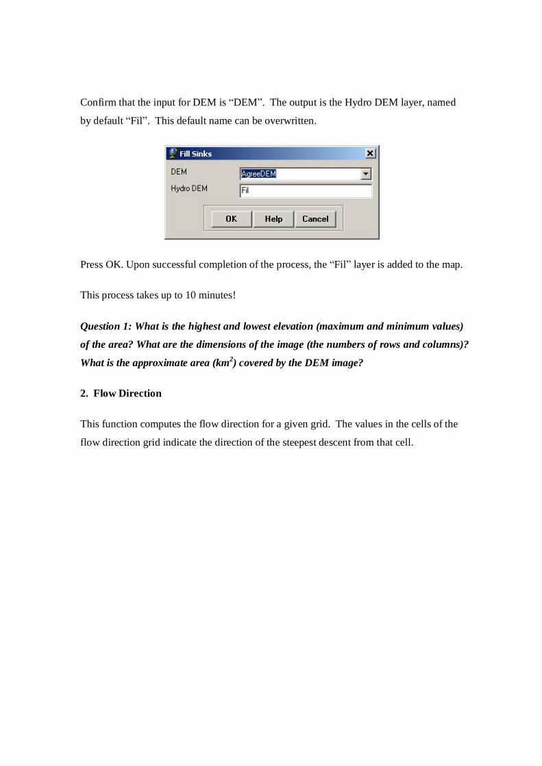
Confirm that the input for DEM is “DEM”. The output is the Hydro DEM layer, named
by default “Fil”. This default name can be overwritten.
Press OK. Upon successful completion of the process, the “Fil” layer is added to the map.
This process takes up to 10 minutes!
Question 1: What is the highest and lowest elevation (maximum and minimum values)
of the area? What are the dimensions of the image (the numbers of rows and columns)?
What is the approximate area (km2) covered by the DEM image?
2. Flow Direction
This function computes the flow direction for a given grid. The values in the cells of the
flow direction grid indicate the direction of the steepest descent from that cell.

Select Terrain Preprocessing | Flow Direction.
Confirm that the input for Hydro DEM is “Fil”. The output is the Flow Direction Grid,
named by default “Fdr”. This default name can be overwritten.
Press OK. Upon successful completion of the process, the flow direction grid “Fdr” is
added to the map.
Question 2: Make a screen capture of the attribute table of Fdr and give an
interpretation for the values in the Value field. Explain the main flow directions in the
area.
3. Flow Accumulation
This function computes the flow accumulation grid that contains the accumulated number
of cells upstream of a cell, for each cell in the input grid.
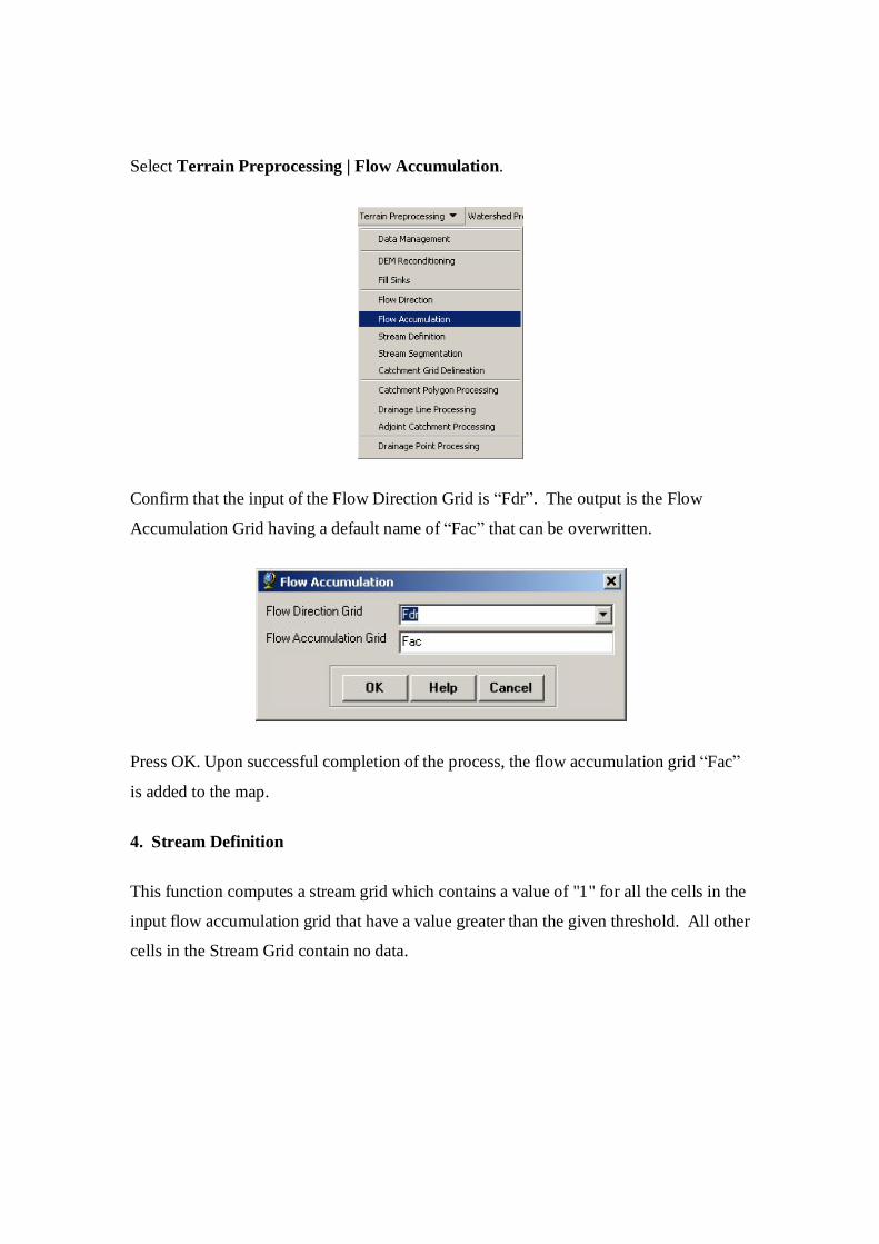
Select Terrain Preprocessing | Flow Accumulation.
Confirm that the input of the Flow Direction Grid is “Fdr”. The output is the Flow
Accumulation Grid having a default name of “Fac” that can be overwritten.
Press OK. Upon successful completion of the process, the flow accumulation grid “Fac”
is added to the map.
4. Stream Definition
This function computes a stream grid which contains a value of "1" for all the cells in the
input flow accumulation grid that have a value greater than the given threshold. All other
cells in the Stream Grid contain no data.
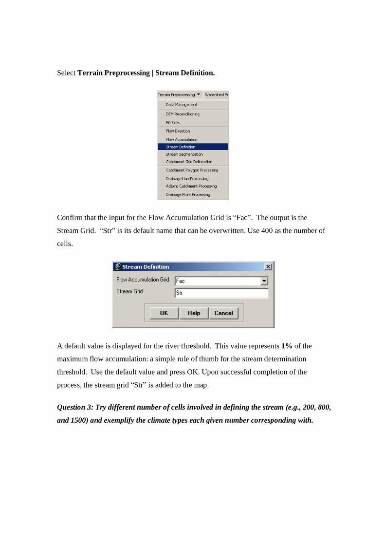
Select Terrain Preprocessing | Stream Definition.
Confirm that the input for the Flow Accumulation Grid is “Fac”. The output is the
Stream Grid. “Str” is its default name that can be overwritten. Use 400 as the number of
cells.
A default value is displayed for the river threshold. This value represents 1% of the
maximum flow accumulation: a simple rule of thumb for the stream determination
threshold. Use the default value and press OK. Upon successful completion of the
process, the stream grid “Str” is added to the map.
Question 3: Try different number of cells involved in defining the stream (e.g., 200, 800,
and 1500) and exemplify the climate types each given number corresponding with.
5. Stream Segmentation
This function creates a grid of stream segments that have a unique identification. Either a
segment may be a head segment, or it may be defined as a segment between two segment
junctions. All the cells in a particular segment have the same grid code that is specific to
that segment.
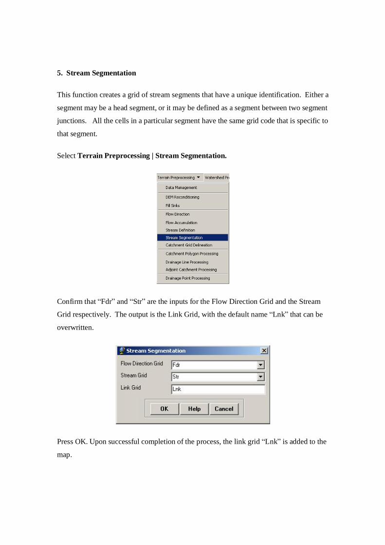
Select Terrain Preprocessing | Stream Segmentation.
Confirm that “Fdr” and “Str” are the inputs for the Flow Direction Grid and the Stream
Grid respectively. The output is the Link Grid, with the default name “Lnk” that can be
overwritten.
Press OK. Upon successful completion of the process, the link grid “Lnk” is added to the
map.

6. Catchment Grid Delineation
This function creates a grid in which each cell carries a value (grid code) indicating to
which catchment the cell belongs. The value corresponds to the value carried by the
stream segment that drains that area, defined in the stream segment link grid
Select Terrain Preprocessing | Catchment Grid Delineation.
Confirm that the input to the Flow Direction Grid and Link Grid are “Fdr” and “Lnk”
respectively. The output is the Catchment Grid layer. “Cat” is its default name that can
be overwritten by the user.
Press OK. Upon successful completion of the process, the Catchment grid “Cat” is added
to the map. You can recolor it with Unique Values to get a nice display.
Question 4: Create a histogram to show the relationships between total length of each
stream segment and area of corresponding catchment. The X and Y represent the
length of stream segment and cumulative area of catchment basin. Explain your result.
7. Catchment Polygon Processing
This function converts a catchment grid into a catchment polygon feature.
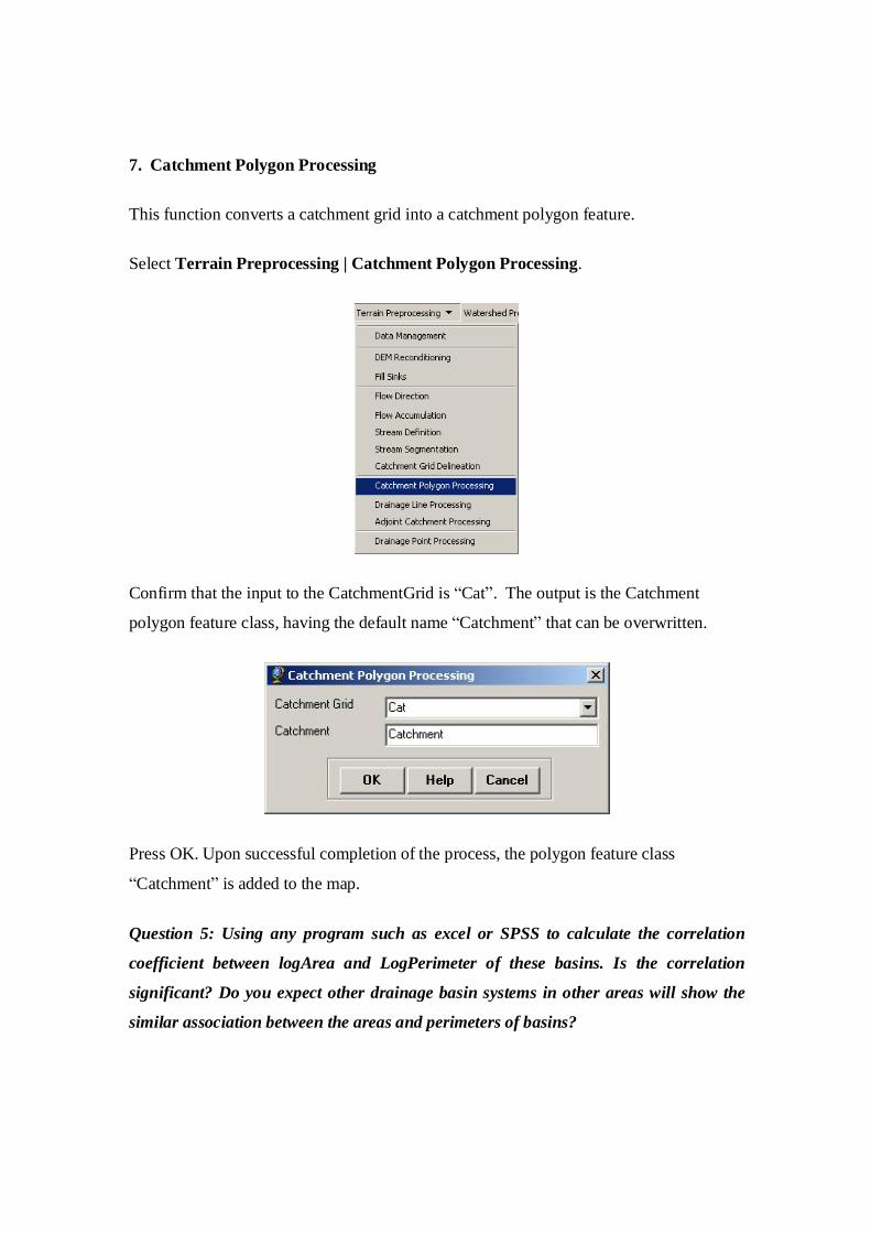
Select Terrain Preprocessing | Catchment Polygon Processing.
Confirm that the input to the CatchmentGrid is “Cat”. The output is the Catchment
polygon feature class, having the default name “Catchment” that can be overwritten.
Press OK. Upon successful completion of the process, the polygon feature class
“Catchment” is added to the map.
Question 5: Using any program such as excel or SPSS to calculate the correlation
coefficient between logArea and LogPerimeter of these basins. Is the correlation
significant? Do you expect other drainage basin systems in other areas will show the
similar association between the areas and perimeters of basins?

8. Drainage Line Processing
This function converts the input Stream Link grid into a Drainage Line feature class.
Each line in the feature class carries the identifier of the catchment in which it resides.
Select Terrain Preprocessing | Drainage Line Processing.
Confirm that the input to Link Grid is “Lnk” and to Flow Direction Grid “Fdr”. The
output Drainage Line has the default name “DrainageLine”, that can be overwritten.
Press OK. Upon successful completion of the process, the linear feature class
“DrainageLine” is added to the map.
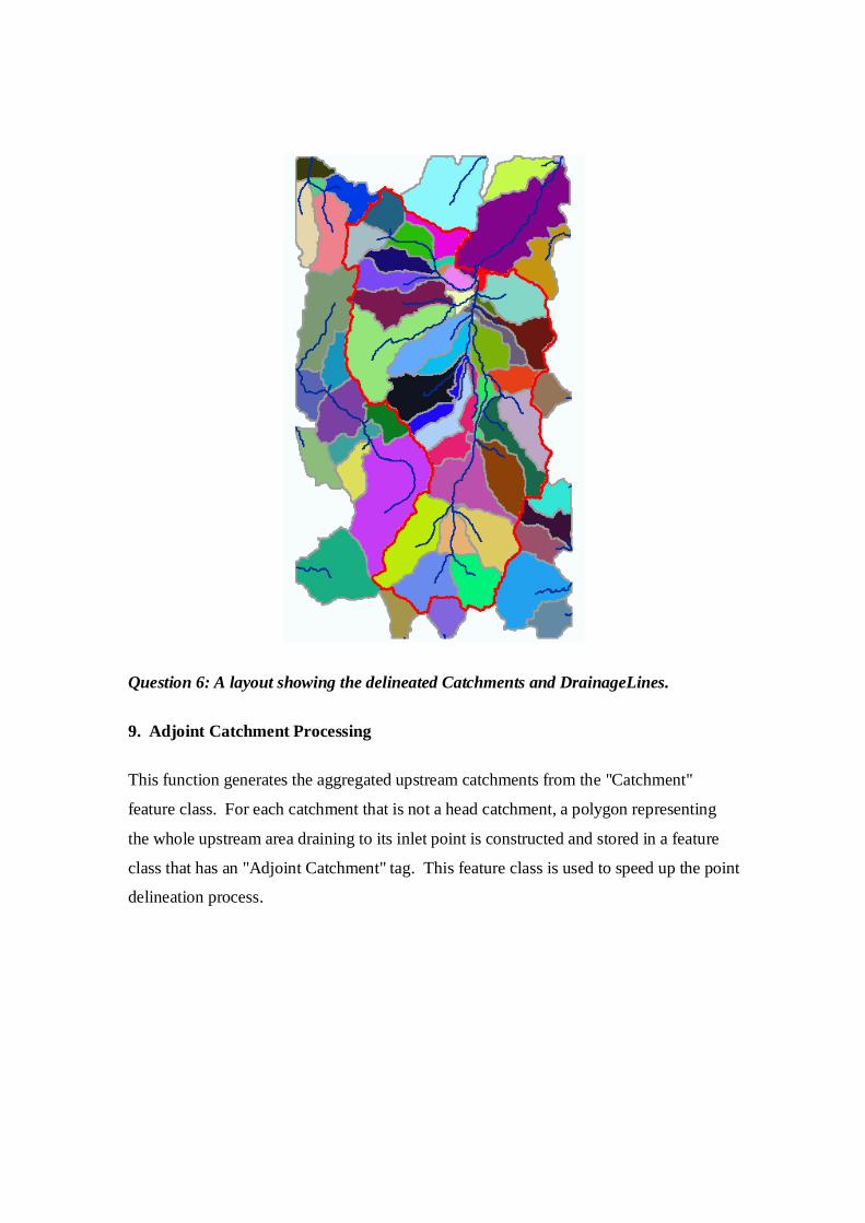
Question 6: A layout showing the delineated Catchments and DrainageLines.
9. Adjoint Catchment Processing
This function generates the aggregated upstream catchments from the "Catchment"
feature class. For each catchment that is not a head catchment, a polygon representing
the whole upstream area draining to its inlet point is constructed and stored in a feature
class that has an "Adjoint Catchment" tag. This feature class is used to speed up the point
delineation process.
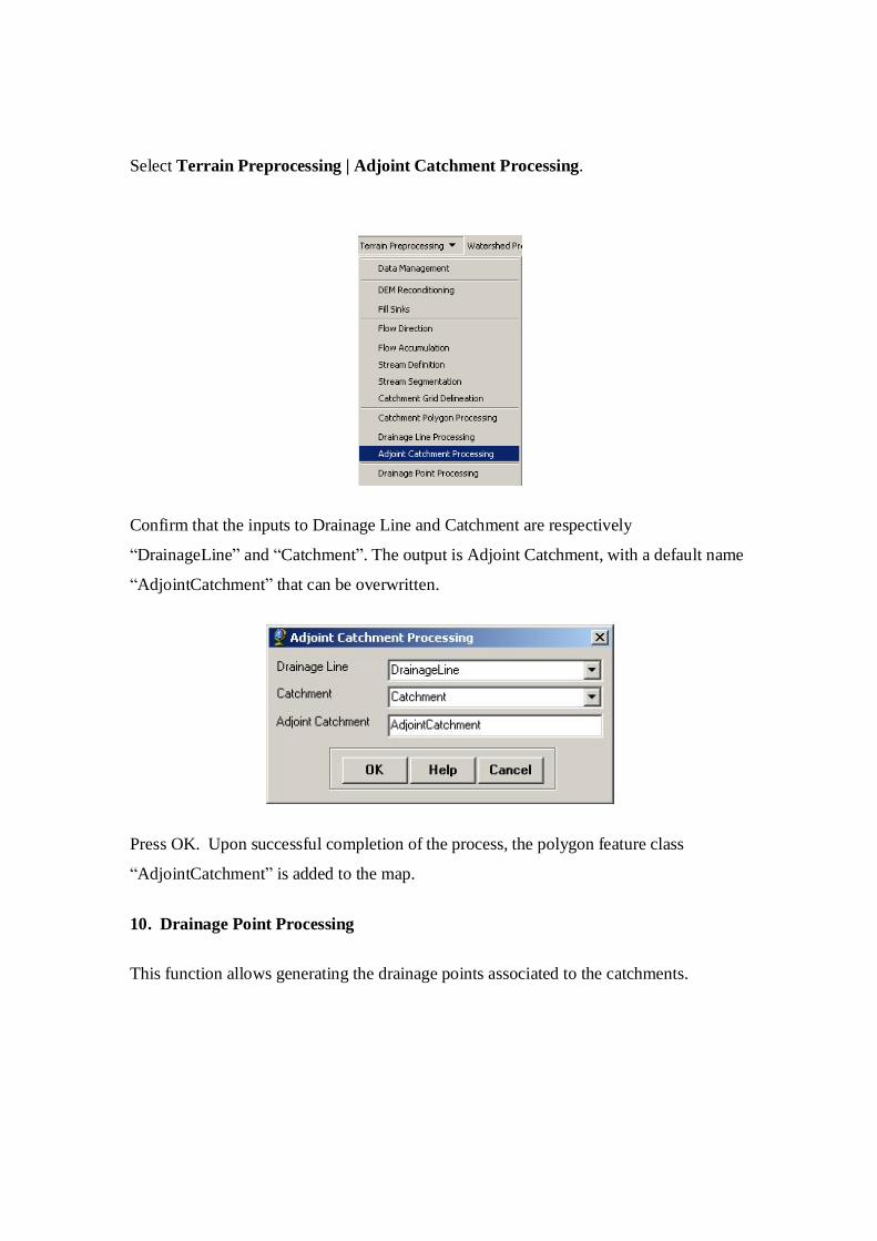
Select Terrain Preprocessing | Adjoint Catchment Processing.
Confirm that the inputs to Drainage Line and Catchment are respectively
“DrainageLine” and “Catchment”. The output is Adjoint Catchment, with a default name
“AdjointCatchment” that can be overwritten.
Press OK. Upon successful completion of the process, the polygon feature class
“AdjointCatchment” is added to the map.
10. Drainage Point Processing
This function allows generating the drainage points associated to the catchments.
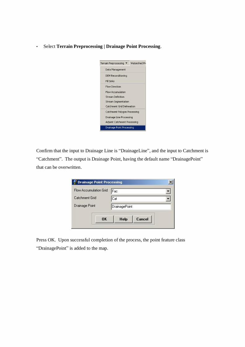
• Select Terrain Preprocessing | Drainage Point Processing.
Confirm that the input to Drainage Line is “DrainageLine”, and the input to Catchment is
“Catchment”. The output is Drainage Point, having the default name “DrainagePoint”
that can be overwritten.
Press OK. Upon successful completion of the process, the point feature class
“DrainagePoint” is added to the map.

Question 7: How many DrainagePoints, DrainageLines and Catchments are there?
What is the ID field in each feature class that associates the appropriate DrainagePoint
with its DrainageLine and Catchment?
Watershed Processing
Now, lets explore the data that we’ve created. Turn off all the themes in the display,
except for the original Digital Elevation Model. From the Arc Hydro tools, select the
Flow Path Tracing button and click on a few places on the elevation model. You’ll
see flow paths traced to the watershed outlet. This path is traced using the Flow
Direction grid created earlier in the exercise.

The flow paths just created are graphics. They can be deleted from the map by using the
Select Elements tool in the ArcMap Draw toolbar, drawing a box around
the graphics and then using the Delete key.
Question 8: A screenshot showing drainage paths traced over the digital elevation model.
Now lets take a look at the Flow Accumulation. Turn on the Fac Grid, and the
DrainageLine theme. Make a Drainage Path trace, and notice how the path follows the
drainage lines.
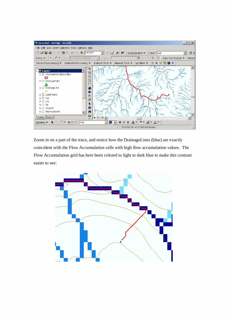
Zoom in on a part of the trace, and notice how the DrainageLines (blue) are exactly
coincident with the Flow Accumulation cells with high flow accumulation values. The
Flow Accumulation grid has here been colored to light to dark blue to make this contrast
easier to see:
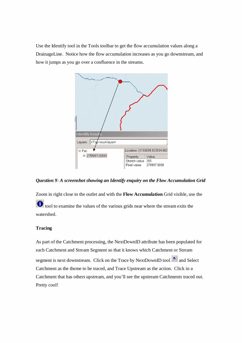
Use the Identify tool in the Tools toolbar to get the flow accumulation values along a
DrainageLine. Notice how the flow accumulation increases as you go downstream, and
how it jumps as you go over a confluence in the streams.
Question 9: A screenshot showing an Identify enquiry on the Flow Accumulation Grid
Zoom in right close to the outlet and with the Flow Accumulation Grid visible, use the
tool to examine the values of the various grids near where the stream exits the
watershed.
Tracing
As part of the Catchment processing, the NextDownID attribute has been populated for
each Catchment and Stream Segment so that it knows which Catchment or Stream
segment is next downstream. Click on the Trace by NextDownID tool and Select
Catchment as the theme to be traced, and Trace Upstream as the action. Click in a
Catchment that has others upstream, and you’ll see the upstream Catchments traced out.
Pretty cool!
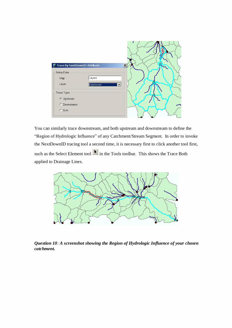
You can similarly trace downstream, and both upstream and downstream to define the
“Region of Hydrologic Influence” of any Catchment/Stream Segment. In order to invoke
the NextDownID tracing tool a second time, it is necessary first to click another tool first,
such as the Select Element tool in the Tools toolbar. This shows the Trace Both
applied to Drainage Lines.
Question 10: A screenshot showing the Region of Hydrologic Influence of your chosen catchment.