Geodesics on an ellipsoid in Minkowski space

Daniel Genin,∗ Boris Khesin† and Serge Tabachnikov‡

May 1, 2007

Abstract

We describe the geometry of geodesics on a Lorentz ellipsoid: giveexplicit formulas for the first integrals (pseudo-confocal coordinates),curvature, geodesically equivalent Riemannian metric, the invariantarea-forms on the time- and space-like geodesics and invariant 1-formon the space of null geodesics. We prove a Poncelet-type theoremfor null geodesics on the ellipsoid: if such a geodesic close up afterseveral oscillations in the “pseudo-Riemannian belt”, so do all othernull geodesics on this ellipsoid.

1 Introduction

The geodesic flow on the ellipsoid in Euclidean space is a classical exam-ple of a completely integrable dynamical system whose study goes back toJacobi and Chasles. We refer to [3, 13, 15] for a modern treatment of thissubject; see also [1, 5, 9, 10, 17, 22] for a sampler of recent work. In arecent paper [12], we considered ellipsoids in pseudo-Euclidean spaces of ar-bitrary signatures and extended, with appropriate adjustments, the theoremon complete integrability of the geodesic flow to this case. We also defined

∗Department of Mathematics, Pennsylvania State University, University Park, PA16802, USA; e-mail: genin@math.psu.edu

†Department of Mathematics, University of Toronto, Toronto, ON M5S 2E4, Canada;e-mail: khesin@math.toronto.edu

‡Department of Mathematics, Pennsylvania State University, University Park, PA16802, USA; e-mail: tabachni@math.psu.edu

1

pseudo-Euclidean billiards and proved that the billiard map inside an ellip-soid in pseudo-Euclidean space is completely integrable.

This note is devoted to the “case study” of geodesics on an ellipsoid inthree dimensional space with the metric dx2 + dy2 − dz2. Recall that thepseudo-sphere x2 + y2 − z2 = −1 in Minkowski space provides a famousexample of a Riemannian metric of constant negative curvature, a modelof the hyperbolic plane, and this gives a further motivation to investigatequadratic surfaces in Minkowski space.

We shall study an ellipsoid

x2

a+

y2

b+

z2

c= 1, a, b, c > 0, (1)

and we assume that the general position condition a > b holds. The inducedmetric 〈 , 〉 on the ellipsoid degenerates along the two curves

z = ±c

√x2

a2+

y2

b2(2)

that will be referred to as the “tropics”. The induced metric is Riemannianin the “polar caps” and Lorentz in the “equatorial belt” bounded by thetropics. We shall see in Section 6 that the Gauss curvature of the ellipsoidis everywhere negative (it equals −∞ on the tropics). At every point of theequatorial belt, one has two null directions of the Lorentz metric; on thetropics, these directions merge together.

Every geodesic curve γ(t) on the ellipsoid (1) is of one of the three types:space-like (positive energy 〈γ′, γ′〉 > 0), time-like (negative energy 〈γ′, γ′〉 <0) or light-like (zero energy or null 〈γ′, γ′〉 = 0). The last two types existonly in the equatorial belt. In fact, a whole new phenomenon which we aredealing with in the Lorentz case, as compared to the Euclidean one, is thepresence of null geodesics, which “separate” the space-like and time-like ones.This makes the pseudo-Riemannian geometry of the problem quite peculiar,and rather different from its Riemannian counterpart.

Let us summarize some relevant results from [12], specialized to thethree dimensional case. Include the ellipsoid into a pseudo-confocal family ofquadrics Mλ given by the equation

x2

a + λ+

y2

b + λ+

z2

c− λ= 1. (3)

It is shown in [12] that:

2

1. Through every generic point Q(x, y, z) in space, there pass either threeor one pseudo-confocal quadrics. In the former case, two of the quadricshave the same topological type, and the quadrics are pairwise orthog-onal at point Q. If Q is a generic point of the ellipsoid (1) then thereexists another pseudo-confocal ellipsoid and a pseudo-confocal hyper-boloid of one sheet, passing through x.

2. A generic space- or time-like line ` is tangent to either two or no pseudo-confocal quadrics. In the former case, the tangent planes to thesequadrics at the tangency points with ` are pairwise orthogonal. Inparticular, a generic line, tangent to the ellipsoid (1), is tangent toanother pseudo-confocal quadric.

3. The tangent lines to a given space-like or time-like geodesic on theellipsoid (1) forever remain tangent to a fixed pseudo-confocal quadric;the respective value of λ in (3) can be considered as an integral of thegeodesic flow.

The spaces of space- or time-like lines in pseudo-Euclidean space, andmore generally, the spaces of space- or time-like geodesics in a pseudo-Riemannian manifold, carry symplectic structures. These structures are ob-tained by symplectic reduction: restrict the canonical symplectic structureof the (co)tangent bundle to the unit energy hypersurface 〈v, v〉 = ±1 andquotient out the one-dimensional kernel of this restriction. In the case of apseudo-Riemannian (Lorentz) surface, we obtain an area form on the set ofspace- and time-like geodesics.1

Now, to billiards. In general, the billiard dynamical system in a pseudo-Riemannian manifold with a smooth boundary describes the motion of a freemass-point (“billiard ball”). The point moves along a geodesic with constantenergy until it hits the boundary where the elastic reflection occurs: thenormal component of the velocity instantaneously changes sign whereas thetangential component remains the same, see [20, 21] for general information.The billiard reflection is not defined at the points where the normal vectoris tangent to the boundary. The billiard ball map acts on oriented geodesicsand takes the incoming trajectory of the billiard ball to the outgoing one.

1It is shown in [12] that the space of light-like geodesics has a contact structure; it istrivial in the case of a surface, as light-like geodesics form a one-dimensional set, and weshall not use this structure in the present paper.

3

This map preserves the type of a geodesic (space-, time-, or light-like). Fur-thermore, the billiard ball map, acting on the space- or time-like geodesics,preserves the symplectic structure (area form, in two-dimensional case) de-scribed above.2

It is proved in [12] that the billiard ball map with respect to a quadricin Minkowski space is integrable as well: if an incoming space- or time-like billiard trajectory is tangent to two pseudo-confocal quadrics then theoutgoing trajectory remains tangent to the same two quadrics.

In general, complete integrability of a billiard system implies configura-tion theorems for closed billiard trajectories, see, e.g., [20, 21]. In particular,the integrability of the billiard inside an ellipse implies the classical PonceletPorism depicted in figure 1: let γ ⊂ Γ be two nested ellipses and let a pointof Γ be a vertex of an n-gon inscribed in Γ and circumscribed about γ; thenevery point of Γ is a vertex of such an n-gon, see [8]...........................................................................................................................................................................................................................................................................................................................................................................................................................................................................................................................................................................................................................................................................................................................................................................................................................................................................................................................................................................................................................................................................................................................................................................................................................................................................................................................................................................................................................................................................................................................................................................................................................................................................................................................................................................................................................................................................................................................................................................................................................................................................................................................................................................................................................................................

..................................................................................................................................................................................................................................................................................................................................................................................................................................................................................................................................................................................................................................................................

......................................................................................................................................................................................................................................................................................................................................................................................................................................................................................................................................................................................................................................................................................................................................................................................................................................................................................................................................................................................................................................................................................................................................................................................................................................................................................................................................................................................................................................................................................................................................................................................................................................

................................................................................................................................................................................................................................................................................................................................................................................................................................................................................................................................................................................................................................................................................................................................................................................................................................................................................................................................................................................................................................................................................................................................................................................................................................................................................................................................................................................................................

.............................................................................................................................................................................................................................................................................................................................................................................................................................................................................................................................................................................................................................................................................................................................................................................................................................................................................................................................................................................................................................................................................................................................................................................................................................................................................................................................................................................................................................................................................................................................................................................................................................................................................................................................................................................................................................................................................................................................................................................................................................................................................................................................................................................................................................................................................................................................................................................................................................................................................................................................................................................................................................................................................................................................................................................................................................................................................................................................

............................................................................................................................................................................................................................................................................................................................................................................................................................................................................................................................................................................................................................

................................................................................................ ........................................................................................................................................................................................................................................................................................................................................................................................................................................................................................................................................................................................................................................................................................................................................................................................................................................................

............................................................................................................................................................................................................................................................................................................................................................................................................................................................................................................................................................................................................................................................................................................................................................................................................................................................................................................................................................................

....................................................................................................................................................................................................................................................................................................................................................................................

Figure 1: Poncelet Porism

In Section 5 we prove a Poncelet-style closure theorem involving nullgeodesics on the ellipsoid: if some chain of such geodesics in the equatorialbelt closes up after n oscillations between the tropics then so does every suchchain.

It is proved in [12] that the billiard inside an ellipse in the Lorentz planeis completely integrable as well. Restricted to light-like lines, the billiardball map in an oval becomes a circle map depending only on the two nulldirections. In Section 7 we discuss the problem when this map is conjugatedto a rotation.

2And, acting on light-like geodesics, preserves the contact structure.

4

2 Joachimsthal integral

The geodesic flow on the triaxial ellipsoid in Euclidean space possesses theclassical Joachimsthal integral. In this section we describe its pseudo-Euclideanversion. This integral says analytically that the lines tangent to a geodesiccurve on the ellipsoid are tangent to a fixed pseudo-confocal quadric: in thisdimension, all first integrals of the geodesic flow, restricted to a constantenergy hypersurface, are functionally dependent.

Choose a Minkowski normal at point (x, y, z) of the ellipsoid (1) as follows:

N(x, y, z) =(x

a,y

b,−z

c

).

Then

〈N(x, y, z), N(x, y, z)〉 =x2

a2+

y2

b2− z2

c2.

We see that the normal is space-like in the equatorial belt, time-like in thepolar caps and null on the tropics.

Let (u, v, w) denote a tangent vector to the ellipsoid.

Proposition 2.1 The following function is an integral of the geodesic flow:

J =

(x2

a2+

y2

b2− z2

c2

)(u2

a+

v2

b+

w2

c

). (4)

Proof. Parameterized geodesics γ(t) are extrema of the functional∫〈γ(t), γ(t)〉 dt;

they satisfy the Euler-Lagrange equation γ(t) = λ(t)N(γ(t)) where λ(t) is aLagrange multiplier.

Let γ(t) be a geodesic with γ(t) = (u, v, w). Then γ(t) = λ(t)N(γ(t)),and hence

λ(t) =〈γ(t), N(γ(t))〉

〈N(γ(t)), N(γ(t))〉.

Since 〈γ(t), N(γ(t))〉 = 0, we have:

〈γ(t), N(γ(t))〉 = −〈γ(t), N(γ(t))〉 = −〈(u, v, w),(u

a,v

b,−w

c

)〉 = −

(u2

a+

v2

b+

w2

c

),

5

and it follows that

λ(t) = −u2

a+ v2

b+ w2

c

x2

a2 + y2

b2− z2

c2

(5)

(the denominator vanishes precisely on the tropics).We want to prove that J = 0. Indeed,

2J =(xu

a2+

yv

b2− zw

c2

)(u2

a+

v2

b+

w2

c

)+

(x2

a2+

y2

b2− z2

c2

)(uu

a+

vv

b+

ww

c

)

=(xu

a2+

yv

b2− zw

c2

)(u2

a+

v2

b+

w2

c

)+λ

(x2

a2+

y2

b2− z2

c2

)(xu

a2+

yv

b2− zw

c2

)= 0,

the last equality due to (5). 2

3 Describing the geodesics

3.1 Global behavior of geodesics

As we mentioned earlier, the metric in the polar caps is Riemannian, whilein the equatorial belt it is Lorentzian. A geodesic in a polar cap crosses itfrom tropic to tropic.

Consider the equatorial belt. The light-like geodesics traverse the beltfrom one tropic to another. There are two kinds of them depending onthe slope, positive or negative; we call these null geodesics right and left,respectively. The time-like geodesics are squeezed between like-like ones andhence also go from tropic to tropic.

Let us discuss the behavior of space-like geodesics. The equator is a closedgeodesic. Figure 2 depicts two other space-like geodesics (first two pictures);the first one intersects the equator and proceeds to the other tropic, andthe other geodesic starts at a tropic and returns to the same tropic withoutreaching the equator. These two geodesics represent generic behavior as thenext lemma shows.

Lemma 3.1 Let γ(t) = (x(t), y(t), z(t)) be a geodesic in the Northern partof the equatorial belt, i.e., z(t) > 0. Then z(t) > 0. In the Southern part ofthe equatorial belt, z(t) < 0

6

Figure 2: Space-like geodesics in the equatorial belt

Proof. Since γ(t) = λ(t)N(γ(t)), we have: z(t) = −λ(t)z(t)/c. Accordingto (5), λ < 0 in the equatorial belt, hence z(t) > 0 for z > 0 (i.e., in theNorthern part) and z(t) < 0 for z < 0 (in the Southern part). 2

It follows that a geodesic in the Northern part of the equatorial belt isconvex downwards, and in the Southern part of the equatorial belt is convexupwards. It also follows from the proof that the equator, as a closed geodesic,is exponentially unstable.

An intermediate position between the two types of generic space-likegeodesics is occupied by the geodesics that start at, say, Northern tropicand monotonically descend to the equator having the latter as a limit cycle,see figure 2, on the right.

3.2 Local behavior of geodesics near the tropics

The behavior of geodesics near tropics is described by the following

Proposition 3.2 A geodesic on the ellipsoid (1) may reach a tropic only inthe null direction.

7

Proof. For light-like geodesics, there is nothing to prove, and a time-likegeodesic is confined in the wedge between two null directions which mergetogether on a tropic. It remains to consider unit energy space-like geodesics.

According to Proposition 2.1, one has, along a geodesic:(x2

a2+

y2

b2− z2

c2

)(u2

a+

v2

b+

w2

c

)= const, u2 + v2 − w2 = 1.

As the point approaches a tropic, the first factor on the left hand side ofthe first equality goes to zero, and hence the second factor blows up. Thedirection of the geodesic does not change if we rescale the tangent vector:

(u, v, w) = µ(u, v, w), µ =

√x2

a2+

y2

b2− z2

c2

maintaining u2 + v2 + w2 = O(1). As (x, y, z) approaches the tropic, we have

u2 + v2 − w2 = µ2 → 0,

therefore the geodesic has the null direction. 2

It follows from Proposition 3.2 that the null lines tangent to the ellipsoidalong the tropics are tangent to infinitely many pseudo-confocal quadrics.Indeed, infinitely many geodesic hit the tropics at any given point in thenull direction, and the tangent lines to each geodesic are tangent to a fixedpseudo-confocal quadric, see Section 1. In contrast, we have the followingproposition which provides an alternative proof of Proposition 3.2.

Proposition 3.2′ Let P be a point of a tropic and ` a space-like line tangentto the ellipsoid at P . Then ` is not tangent to any pseudo-confocal quadric.

Proof. Assume that ` is tangent to Mλ at point Q. Denote by N a normalvector to M0 at P and by η a normal vector to Mλ at Q. Then N lies in thetangent plane TP M0. The restriction of the ambient metric to this plane isdegenerate, and N spans the kernel of this restriction.

According to the general theory, see Section 1, η is orthogonal to N , henceη lies in N⊥ = TP M0. Since η is also orthogonal to `, the normals η and Nare collinear. Therefore the tangent planes TP M0 and TQMλ coincide.

The projection of pseudo-confocal family along the line ` is a pseudo-confocal family of conics in the Lorentz plane, see [12]. It follows that the

8

Figure 3: Pseudo-confocal family of conics x2

1+λ+ y2

1−λ= 1

projections of M0 and Mλ are tangent to each other. However no two conicsin a pseudo-confocal family are tangent (see figure 3), a contradiction. 2

Proposition 3.2 is a manifestation of a more general phenomenon whichholds for Lorentz surfaces. Suppose, on an analytic Lorentz surface S, theLorentz metric changes into Riemannian (i.e., the two null direction coincide)along a smooth curve Γ. We call a point of Γ regular if the null direction atthis point is transversal to the curve Γ itself.

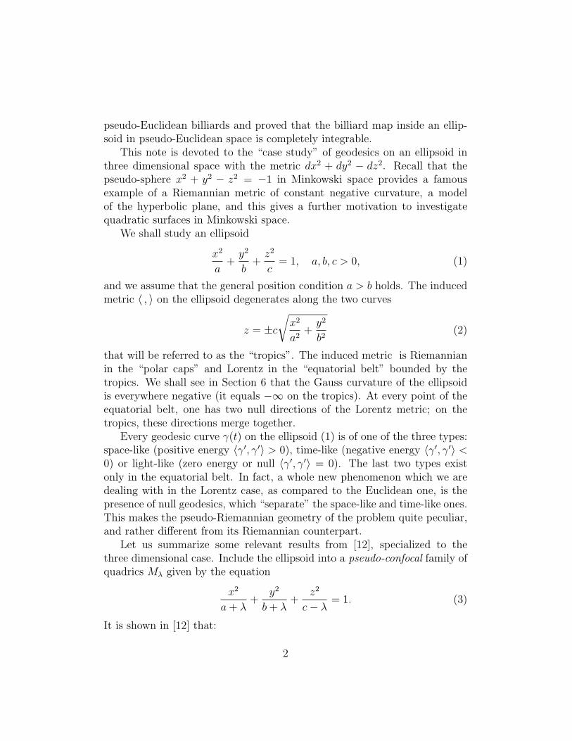
Proposition 3.3 In a neighborhood of a regular point the Lorentz metric onthe surface S is conformally equivalent to the metric dy2−x dx2 in a neighbor-hood of the origin. The null geodesics on S near this point are diffeomorphicto the family of cusps y = x3/2 + C, see figure 4.

Proof. Let a(x, y)dx2 + b(x, y)dxdy + c(x, y)dy2 be a Lorentz metric on S.Then the equation of null geodesics on S is a(x, y)+b(x, y)y′+c(x, y)(y′)2 = 0,an implicit differential equation of the first order. The condition of transver-sality at a regular point of Γ means that we consider a so-called “regularsingular point” of the implicit differential equation F (x, y, y′) = 0. Accord-ing to the theorem of Cibrario (see a discussion in [2]) the normal form ofthis differential equation at a regular singular point is (y′)2 = x, which is theequation of null geodesics in the metric dy2 − x dx2. Thus the null geodesicsis the family of cusps described above.

9

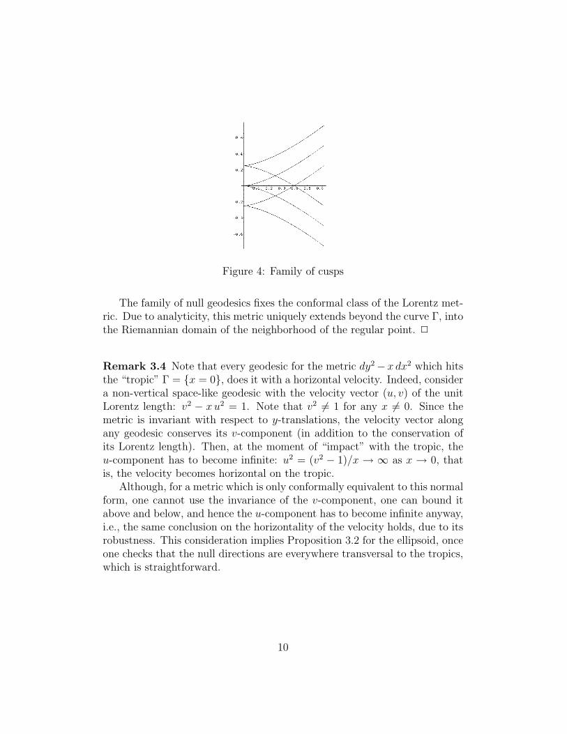
Figure 4: Family of cusps

The family of null geodesics fixes the conformal class of the Lorentz met-ric. Due to analyticity, this metric uniquely extends beyond the curve Γ, intothe Riemannian domain of the neighborhood of the regular point. 2

Remark 3.4 Note that every geodesic for the metric dy2−x dx2 which hitsthe “tropic” Γ = {x = 0}, does it with a horizontal velocity. Indeed, considera non-vertical space-like geodesic with the velocity vector (u, v) of the unitLorentz length: v2 − x u2 = 1. Note that v2 6= 1 for any x 6= 0. Since themetric is invariant with respect to y-translations, the velocity vector alongany geodesic conserves its v-component (in addition to the conservation ofits Lorentz length). Then, at the moment of “impact” with the tropic, theu-component has to become infinite: u2 = (v2 − 1)/x → ∞ as x → 0, thatis, the velocity becomes horizontal on the tropic.

Although, for a metric which is only conformally equivalent to this normalform, one cannot use the invariance of the v-component, one can bound itabove and below, and hence the u-component has to become infinite anyway,i.e., the same conclusion on the horizontality of the velocity holds, due to itsrobustness. This consideration implies Proposition 3.2 for the ellipsoid, onceone checks that the null directions are everywhere transversal to the tropics,which is straightforward.

10

3.3 Intersections with pseudo-confocal quadrics

The topology of a pseudo-confocal quadric (3) depends on the position of λrelative the three numbers −a,−b and c: if λ < −a then Mλ is a hyperboloidof two sheets, if −a < λ < −b then Mλ is a hyperboloid of one sheet, if−b < λ < c then Mλ is an ellipsoid, and if c < λ then Mλ is again ahyperboloid of one sheet. Only the second and the third kinds intersect theoriginal ellipsoid, M0. See figure 5 for all five quadrics and figure 6 for anellipsoid Mλ with −b < λ < c intersecting M0.

Figure 5: Four pseudo-confocal quadrics, along with the initial ellipsoid

The intersection curve Γλ = M0 ∩Mλ is given by the equation

x2

a(a + λ)+

y2

b(b + λ)=

z2

c(c− λ). (6)

In the limit λ → 0, this becomes the equation of the tropic (2). As λ → c,the curve Γλ tends to the equator. The projection of the intersection curve

11

Figure 6: A pseudo-confocal ellipsoid intersecting the initial one

Γλ on the (x, y)-plane is a conic

a + c

a(a + λ)x2 +

b + c

b(b + λ)y2 = 1.

If −a < λ < −b then this conic is a hyperbola, and if −b < λ < c it is anellipse.

Fix a value of λ. Given a generic point P of the ellipsoid M0, the numberof tangent lines from P to the conic TP M0 ∩ Mλ may equal 2 or 0, andthe curve Γλ separates these two domains, say, Uλ and Vλ (the number oftangents equals 1 for P ∈ Γλ).

Consider a geodesic γ on M0. The lines tangent to γ are tangent tosome pseudo-confocal quadric Mλ. Therefore γ is confined to Uλ and, at anypoint P ∈ Uλ, the geodesic γ may have only two directions: the tangentdirections from P to the conic TP M0 ∩Mλ. The geodesic γ cannot intersectthe boundary Γλ but can touch it.

Note that the equator plays a special role: no line tangent to the equatoris tangent to any pseudo-confocal quadric (except M0). Indeed, such a linelies in the horizontal plane, and the trace of the pseudo-confocal family (3)in the horizontal plane is the confocal family of conics. But confocal conicshave no common tangents.

3.4 Reflection of geodesics off the tropics

Define “reflection” of a geodesic γ off a tropic as the geodesic tangent to thesame pseudo-confocal quadric as γ or, equivalently, having the same value

12

of the Joachimsthal integral (normalizing the energy to ±1). According toProposition 3.2, a geodesic and a reflected one have the null direction at theimpact point and hence are tangent to each other.

Proposition 3.5 1). Let γ be a geodesic in a polar cap tangent to a curveΓλ = M0∩Mλ, and let γ1 be the reflection of γ in the tropic. Then γ1 is alsotangent to Γλ (see figure 7).2). Let γ be a space-like geodesic in the equatorial belt that does not intersectthe equator, and let γ1 be the reflection of γ in the tropic. Then γ is tangentto a curve Γλ, separating γ from the equator, and γ1 is also tangent to Γλ

and therefore disjoint from the equator, see figure 8.

Figure 7: Reflected geodesics in a polar cap

Proof. Since the geodesic γ is tangent to Γλ, the tangent lines to γ aretangent to Mλ. By definition, the tangent lines to γ1 are tangent to Mλ aswell, and hence γ1 will touch Γλ, and the first claim follows.

Likewise, the tangent lines to a space-like geodesic γ in the equatorialbelt are tangent to a pseudo-confocal geodesic Mλ. Since γ does not reachthe equator, the curve Γλ separates the tropic and the equator. Arguing asabove, the reflected geodesic γ1 is also tangent to Γλ and therefore disjointfrom the equator. 2

13

Figure 8: Reflected geodesics in the equatorial belt (unfolded)

3.5 Geodesics on degenerate ellipsoids

It is useful to visualise the degenerations of the ellipsoid (1) into a two-sidedflat surface, “a pancake.” First consider the limit c → 0, under which theellipsoid gets squeezed to an ellipse with semi-axes a and b in the Euclideanplane {z = 0}. Then the (Lorentz) equatorial belt disappears, whereas each(Riemannian) polar cap becomes the interior of an ellipse. The geodesicsin the polar caps become straight lines in the limit, and their reflection offthe tropics becomes the billiard reflection in the ellipse; the Joachimsthalintegral describes the confocal ellipse to which a billiard trajectory remainstangent.

Compare this with the other degeneration, b → 0. In the latter case theellipsoid becomes (the interior of) an ellipse in the Lorentz plane {y = 0}.The polar caps (and tropics) become squeezed to the arcs of the ellipse z > 0and z < 0 in this plane. The equatorial belt becomes the double cover ofthe interior of the ellipse. The geodesics also become straight lines in theLorentz plane. The null geodesics have two prescribed slopes in this plane:x = ±z. We will see that the dynamics of the null geodesics in the ellipsoidis an interesting extension of the corresponding Lorentz billiard inside theellipse, restricted to oriented null lines.

14

4 Area form on the space of geodesics

In this section we compute the area form ω on the space of time-like geodesics,described in Section 1. We also define a 1-form on the space of light-likegeodesics which will play the central role in the next section.

Let us characterize a time-like or a light-like geodesic by its intersectionwith the equator of the ellipsoid (1). The equator is parameterized as Q(t) =(√

a cos t,√

b sin t, 0) for t ∈ R/2πZ. Let a geodesic make (Euclidean) angleα with the equator. Then (t, α) are coordinates in the space of geodesicsintersecting the equator. The null directions correspond to α = π/4 and3π/4, and for time-like geodesics, π/4 < α < 3π/4. We set

f(t) =√

a sin2 t + b cos2 t, τ =1√

tan2 α− 1.

Note that for α = π/2, the value of τ is well-defined: τ = 0. The followingproposition describes the Joachimsthal integral J and the area form ω interms of the (t, α) coordinates.

Proposition 4.1 One has:

J(t, α) =cτ 2 + f 2(t)(1 + τ 2)

abc, ω = f(t)dτ ∧ dt. (7)

Proof. For the tangent vector to the equator, one has:

Q′(t) = (−√

a sin t,√

b cos t, 0), 〈Q′(t), Q′(t)〉 = f 2(t).

The geodesic corresponding to (t, α) has a tangent vector

(−√

a sin t,√

b cos t, f(t) tan α).

If the geodesic is time-like, we normalize the tangent vector so that its squaredlength is −1:

(u, v, w) =

(−√

aτ sin t

f(t),

√bτ cos t

f(t), τ tan α

). (8)

To obtain J , substitute (u, v, w) from (8) and

(x, y, z) = (√

a cos t,√

b sin t, 0) (9)

15

to (4); this yields the first formula (7).Identify the cotangent and tangent bundles via the metric. Then the

canonical symplectic form on the cotangent bundle becomes

ω = du ∧ dx + dv ∧ dy − dw ∧ dz.

Formulas (8) and (9) describe a section of the tangent bundle, and the pullback of the symplectic structure ω is given by the second formula (7). 2

As a consequence of Proposition 4.1, we define a natural 1-form on thespace of null geodesics (this space consists of two disjoint circles correspond-ing to the right and left null geodesics). The set of null geodesics is given, in(t, α) coordinates, by α = π/4 or 3π/4, which corresponds to τ = ∞. Notethat both ω and J blow up as one approaches the space of null geodesics,that is, as τ →∞. However, their ratio is well-defined.

Lemma-Definition 4.2 The 1-form h(t)dt, given by the condition that, inthe limit τ →∞,

d(J1/2) ∧ h(t)dt = ω, (10)

is uniquelly defined. Explicitly, this equation holds for h(t) given by

h(t) = const · f(t)√c + f 2(t)

= const ·

√a sin2 t + b cos2 t

c + a sin2 t + b cos2 t(11)

with an appropriate constant factor.

Proof. Up to a constant multiplier, one has:

J1/2 = τ√

c + f 2(t)

(1 + O

(1

τ 2

)),

hence

dJ1/2 =√

c + f 2(t) dτ + g(t, τ) dt + O

(1

τ 2

)for some function g. Therefore(

dJ1/2 ∧ f(t)√c + f 2(t)

dt

)= ω + O

(1

τ 2

),

as needed. 2

16

5 Poncelet-style closure theorem

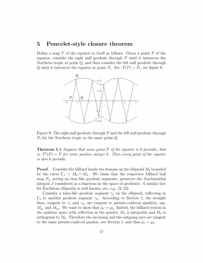
Define a map T of the equator to itself as follows. Given a point P of theequator, consider the right null geodesic through P until it intersects theNorthern tropic at point Q, and then consider the left null geodesic throughQ until it intersects the equator at point P1. Set: T (P ) = P1, see figure 9.

P P1

Q

Figure 9: The right null geodesic through P and the left null geodesic throughP1 hit the Northern tropic at the same point Q.

Theorem 5.1 Suppose that some point P of the equator is k-periodic, thatis, T k(P ) = P for some positive integer k. Then every point of the equatoris also k-periodic.

Proof. Consider the billiard inside the domain on the ellipsoid M0 boundedby the curve Γλ = M0 ∩ Mλ. We claim that the respective billiard ballmap Fλ, acting on time-like geodesic segments, preserves the Joachimsthalintegral J considered as a function on the space of geodesics. A similar factfor Euclidean ellipsoids is well known, see, e.g., [9, 22].

Consider a time-like geodesic segment γ1 on the ellipsoid, reflecting inΓλ to another geodesic segment γ2. According to Section 1, the straightlines, tangent to γ1 and γ2, are tangent to pseudo-confocal quadrics, say,Mµ1 and Mµ2 . We want to show that µ1 = µ2. Indeed, the billiard system inthe ambient space with reflection in the quadric Mλ is integrable and Mλ isorthogonal to M0. Therefore the incoming and the outgoing rays are tangentto the same pseudo-confocal quadric, see Section 1, and thus µ1 = µ2.

17

According to Section 1, Fλ preserves the symplectic structure ω on thespace of time-like geodesics; it also preserves the integral J . Therefore the1-form h(t)dt on the space of null geodesics is also invariant under the actionof the map Fλ on the space of null geodesics.

In the limit λ → 0, the curve Γλ becomes the tropic (2), and the billiardball map Fλ, restricted to null geodesics, gets identified with the map T .Hence T preserves the 1-form h(t)dt.

Finally, choose a cyclic coordinate s on the equator so that h(t)dt = ds.In this coordinate, the map T is a shift s 7→ s + c. This map is k-periodic ifand only if kc ∈ Z. This implies the statement of the theorem. 2

Problem 5.2 It is interesting to find the relation on a, b, c, necessary andsufficient for the orbits of the map T to close up after k iterations and r turnsaround the equator. In the case of the Poncelet Porism, such conditions werefound by Cayley, see [11] for a modern treatment.

Remark 5.3 One also has Poncelet-style closure theorems for the geodesicsin the polar caps and for space- or time-like geodesics in the equatorial beltreflecting from the tropics. Such results are similar to the ones known forEuclidean ellipsoid, see, e.g., [9, 22], and their proofs are similar to that ofTheorem 5.1 but simpler: the T -invariant 1-form h(t)dt is obtained froma finite area form and a finite integral, not as a finite ratio of two infinitequantities.

6 Curvature of the ellipsoid and a geodesi-

cally equivalent Riemannian metric on it

6.1 Curvature of the ellipsoid

The behavior of the geodesics in a polar cap resembles that of the geodesics inthe Poincare disc model of the hyperbolic plane; this observation is explainedby the following proposition.

Proposition 6.1 The Gauss curvature K of the ellipsoid is negative; it isgiven by the formula:

1

K= −abc

(x2

a2+

y2

b2− z2

c2

)2

.

18

Proof. Similarly to the Euclidean case, one can use the normal Gauss mapto compute the Gauss curvature of a surface, see [16]. Consider the Northernpolar cap. Normalize the normal vector as follows:

N(x, y, z) =

(xa, y

b,− z

c

)√z2

c2− x2

a2 − y2

b2

,

so that 〈N, N〉 = −1. Thus the Gauss map sends the polar cap to the uppersheet of the hyperboloid of two sheets, and this map reverses the orientation.Hence the Gauss curvature is negative.

Similarly, one considers the equatorial belt: the normal vector is thennormalized to 〈N, N〉 = 1.

It is straightforward but tedious to compute the Gauss curvature, andwe do not dwell on this. The computation can be simplified by the use ofMathematica. 2

6.2 Riemannian geodesically equivalent metric

The next result follows from general constructions in [14, 19]; for complete-ness, we give a direct proof. Two metrics are called geodesically equivalent ifthey have the same non-parameterized geodesics.

Proposition 6.2 The metric on the ellipsoid (1), induced from the ambientMinkowski space, is geodesically equivalent to the Riemannian metric

ds2 =dx2

a+ dy2

b+ dz2

c∣∣∣x2

a2 + y2

b2− z2

c2

∣∣∣ . (12)

Proof. Let P = (u, v, w) denote a tangent vector at point Q = (x, y, z).Denote the diagonal matrix with the entries (1/a, 1/b, 1/c) by A. To fix ideas,consider the equatorial belt. The Lagrangian for the metric (12) is

L(P, Q) =u2

a+ v2

b+ w2

c

x2

a2 + y2

b2− z2

c2

=A(P ) · P

f(Q)

with

f(Q) =x2

a2+

y2

b2− z2

c2.

19

The Euler-Lagrange equation for a geodesic Q(t) with Q = P is

LPP (Q) + LPQ(P )− LQ = λA(Q)

where A(Q) is a Euclidean normal to the ellipsoid at point Q and λ is aLagrange multiplier; here LPP and LPQ are the matrices of the second partialderivatives and LQ is the gradient vector.

One easily computes:

LPP =2

f(Q)A, LPQ = − 2

f 2(Q)A(P )⊗∇f(Q), LQ = −A(P ) · P

f 2(Q)∇f(Q),

and the Euler-Lagrange equation is rewritten as

A(Q)− P · ∇f(Q)

f(Q)A(P ) +

A(P ) · P2f(Q)

∇f(Q) = λA(Q). (13)

To find the Lagrange multiplier, dot multiply equation (13) by Q. One has:

A(Q) ·Q = 1, A(P ) ·Q = P · A(Q) = 0, ∇f(Q) ·Q = 2f(Q),

and hence

λ = A(Q) ·Q + A(P ) · P =d(A(P ) ·Q)

dt= 0.

Thus (13) implies that the acceleration Q lies in the plane spanned by thevelocity vector P and the vector A−1(∇f(Q)) = 2N(Q), the Minkowskinormal to the ellipsoid at point Q. It follows that Q(t) is a reparameterizedgeodesic of the restriction of the ambient metric on the ellipsoid.

The case of the polar caps is similar. 2

Remark 6.3 Note that the metric (12) is given by the ratio of the twofactors whose product is the Joachimsthal integral (4).

7 Rigidity of ellipses as integrable Lorentz

billiard curves

In Section 3.5, we considered the limit of the ellipsoid (1) as b → 0. In thislimit, the ellipsoid becomes an ellipse in the Lorentz plane. This ellipse is

20

foliated by two parallel families of null lines, and the map T , defined at thebeginning of Section 5, takes oriented lines in one null direction to orientednull lines in the other one.

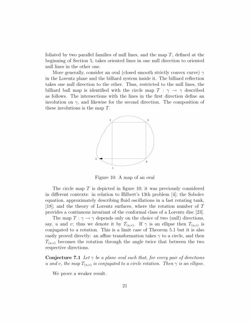
More generally, consider an oval (closed smooth strictly convex curve) γin the Lorentz plane and the billiard system inside it. The billiard reflectiontakes one null direction to the other. Thus, restricted to the null lines, thebilliard ball map is identified with the circle map T : γ → γ describedas follows. The intersections with the lines in the first direction define aninvolution on γ, and likewise for the second direction. The composition ofthese involutions is the map T .

1

2 3

45

Figure 10: A map of an oval

The circle map T is depicted in figure 10; it was previously consideredin different contexts: in relation to Hilbert’s 13th problem [4]; the Sobolevequation, approximately describing fluid oscillations in a fast rotating tank,[18]; and the theory of Lorentz surfaces, where the rotation number of Tprovides a continuous invariant of the conformal class of a Lorentz disc [23].

The map T : γ → γ depends only on the choice of two (null) directions,say, u and v; thus we denote it by T(u,v). If γ is an ellipse then T(u,v) isconjugated to a rotation. This is a limit case of Theorem 5.1 but it is alsoeasily proved directly: an affine transformation takes γ to a circle, and thenT(u,v) becomes the rotation through the angle twice that between the tworespective directions.

Conjecture 7.1 Let γ be a plane oval such that, for every pair of directionsu and v, the map T(u,v) is conjugated to a circle rotation. Then γ is an ellipse.

We prove a weaker result.

21

Theorem 7.2 Let γ(t) be a parameterized plane oval with the property that,for every pair of directions u and v, the map T is a translation in the variablet, i.e., there is a constant c(u, v) such that T(u,v)(γ(t)) = γ(t+ c(u, v)). Thenγ is an ellipse.

Proof. Without loss of generality, assume that γ is parameterized by t ∈R/2πZ.

Choose a direction u. There is a unique maximal chord of γ in directionu, say, AB; such a chord is called an affine diameter. Since AB is maximal,the tangent lines to γ at A and B are parallel; let v be their direction. It isconvenient to apply an affine transformation that makes u horizontal and vvertical.

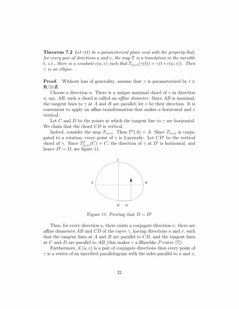
Let C and D be the points at which the tangent line to γ are horizontal.We claim that the chord CD is vertical.

Indeed, consider the map T(u,v). Then T 2(A) = A. Since T(u,v) is conju-gated to a rotation, every point of γ is 2-periodic. Let CD′ be the verticalchord of γ. Since T 2

(u,v)(C) = C, the direction of γ at D′ is horizontal, andhence D′ = D, see figure 11.

A

D’ D

C

B

Figure 11: Proving that D = D′

Thus, for every direction u, there exists a conjugate direction v: there areaffine diameters AB and CD of the curve γ, having directions u and v, suchthat the tangent lines at A and B are parallel to CD, and the tangent linesat C and D are parallel to AB (this makes γ a Blaschke P -curve [7]).

Furthermore, if (u, v) is a pair of conjugate directions then every point ofγ is a vertex of an inscribed parallelogram with the sides parallel to u and v,

22

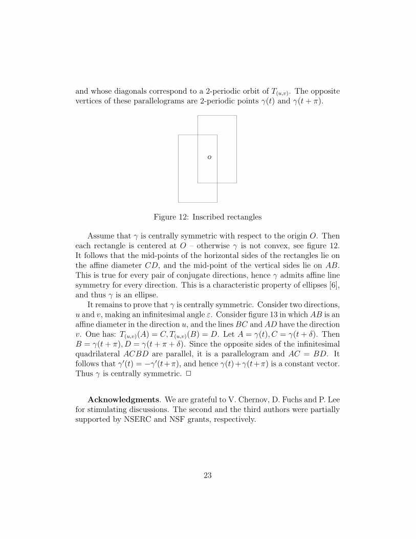
and whose diagonals correspond to a 2-periodic orbit of T(u,v). The oppositevertices of these parallelograms are 2-periodic points γ(t) and γ(t + π).

O

Figure 12: Inscribed rectangles

Assume that γ is centrally symmetric with respect to the origin O. Theneach rectangle is centered at O – otherwise γ is not convex, see figure 12.It follows that the mid-points of the horizontal sides of the rectangles lie onthe affine diameter CD, and the mid-point of the vertical sides lie on AB.This is true for every pair of conjugate directions, hence γ admits affine linesymmetry for every direction. This is a characteristic property of ellipses [6],and thus γ is an ellipse.

It remains to prove that γ is centrally symmetric. Consider two directions,u and v, making an infinitesimal angle ε. Consider figure 13 in which AB is anaffine diameter in the direction u, and the lines BC and AD have the directionv. One has: T(u,v)(A) = C, T(u,v)(B) = D. Let A = γ(t), C = γ(t + δ). ThenB = γ(t + π), D = γ(t + π + δ). Since the opposite sides of the infinitesimalquadrilateral ACBD are parallel, it is a parallelogram and AC = BD. Itfollows that γ′(t) = −γ′(t+π), and hence γ(t)+γ(t+π) is a constant vector.Thus γ is centrally symmetric. 2

Acknowledgments. We are grateful to V. Chernov, D. Fuchs and P. Leefor stimulating discussions. The second and the third authors were partiallysupported by NSERC and NSF grants, respectively.

23

DB

C A

Figure 13: Proving central symmetry of γ

References

[1] S. Abenda, Yu. Fedorov. Closed geodesics and billiards on quadrics re-lated to elliptic KdV solutions. Lett. Math. Phys. 76 (2006), 111–134.

[2] V. Arnold. Geometric methods in the theory of ordinary differential equa-tions, Second edition, Springer-Verlag, 1988, p.27.

[3] V. Arnold, A. Givental. Symplectic geometry, 1-136. Encycl. of Math.Sci., Dynamical Systems, 4, Springer-Verlag, 1990.

[4] V. Arnold. From Hilbert’s superposition problem to dynamical systems,1–18. The Arnoldfest, Amer. Math. Soc., Providence, RI, 1999.

[5] M. Audin. Courbes algebriques et systemes integrables: geodesiques desquadriques, Expos. Math. 12 (1994), 193–226.

[6] M. Berger. Convexity. Amer. Math. Monthly 97 (1990), 650–678.

[7] W. Blaschke. Zur Affingeometrie der Eilinien und Eiflchen. Math.Nachr. 15 (1956), 258–264.

24

[8] H. Bos, C. Kers, F. Oort, D. Raven. Poncelet’s closure theorem. Expos.Math. 5 (1987), 289–364.

[9] S.-J. Chang, K.J. Shi. Billiard systems on quadric surfaces and the Pon-celet theorem. J. Math. Phys. 30 (1989) 798–804.

[10] V. Dragovic, M. Radnovic. Geometry of integrable billiards and pencilsof quadrics. J. Math. Pures Appl. 85 (2006), 758–790.

[11] Ph. Griffiths, J. Harris. On Cayley’s explicit solution to Poncelet’sporism. Enseign. Math. 24 (1978), no. 1-2, 31–40.

[12] B. Khesin, S. Tabachnikov. Spaces of pseudo-Riemannian geodesics andpseudo-Euclidean billiards. Preprint ArXiv math.DG/0608620.

[13] H. Knorrer. Geodesics on the ellipsoid. Invent. Math. 59 (1980), 119–143.

[14] V. Matveev, P. Topalov. Trajectory equivalence and corresponding inte-grals. Reg. Chaotic Dyn. 3 (1998), 30–45.

[15] J. Moser. Various aspects of integrable Hamiltonian systems, 233-289.Progr. in Math. 8, Birhauser, 1980.

[16] B. O’Neill. Semi-Riemannian geometry. With applications to relativity.Academic Press, New York, 1983.

[17] E. Previato. Some integrable billiards. SPT 2002: Symmetry and per-turbation theory, 181–195, World Sci. Publ., 2002.

[18] S. Sobolev. On a new problem of mathematical physics. Izvestia Akad.Nauk SSSR, Ser. Mat. 18 (1954), 3–50.

[19] S. Tabachnikov. Projectively equivalent metrics, exact transverse linefields and the geodesic flow on the ellipsoid. Comm. Math. Helv. 74(1999), 306–321.

[20] S. Tabachnikov. Billiards. Soc. Math. de France, Paris, 1995.

[21] S. Tabachnikov. Geometry and billiards. Amer. Math. Soc., Providence,RI, 2005.

25

[22] A. Veselov. Confocal surfaces and integrable billiards on the sphere andin the Lobachevsky space. J. Geom. Phys. 7 (1990), 81–107.

[23] T. Weinstein. An introduction to Lorentz surfaces. Walter de Gruyter &Co., Berlin, 1996.

26